Human Mobility Prediction with Causal and Spatial-constrained Multi-task Network

Abstract.

Modeling human mobility helps to understand how people are accessing resources and physically contacting with each other in cities, and thus contributes to various applications such as urban planning, epidemic control, and location-based advertisement. Next location prediction is one decisive task in individual human mobility modeling and is usually viewed as sequence modeling, solved with Markov or RNN-based methods. However, the existing models paid little attention to the logic of individual travel decisions and the reproducibility of the collective behavior of population. To this end, we propose a Causal and Spatial-constrained Long and Short-term Learner (CSLSL) for next location prediction. CSLSL utilizes a causal structure based on multi-task learning to explicitly model the ”when$\rightarrow$what$\rightarrow$where”, a.k.a. ”time$\rightarrow$activity$\rightarrow$location” decision logic. We next propose a spatial-constrained loss function as an auxiliary task, to ensure the consistency between the predicted and actual spatial distribution of travelers’ destinations. Moreover, CSLSL adopts modules named Long and Short-term Capturer (LSC) to learn the transition regularities across different time spans. Extensive experiments on three real-world datasets show promising performance improvements of CSLSL over baselines and confirm the effectiveness of introducing the causality and consistency constraints. The implementation is available at https://github.com/urbanmobility/CSLSL.

1. Introduction

Human mobility modeling aims to explore the regularities and patterns of human behavior (Gonzalez et al., 2008; Barbosa et al., 2018) and plays a significant role in numerous applications, such as urban planning (Xu et al., 2021), travel demand management (Çolak et al., 2016; Xu et al., 2018), health risk assessment (Xu et al., 2019), epidemic spreading modeling and control (Arenas et al., 2020; Jia et al., 2020), and so on. In the big data era, the accessibility to GPS, mobile phone records, and location-based social networks (LBSNs) provides an unprecedented chance to understand and model human mobility (Barbosa et al., 2018; Luca et al., 2020).

In the research community of human mobility, physicists focus on statistical analysis from a macroscopic perspective and have summarized empirical rules (Barbosa et al., 2018). For example, they found that, truncating the power law distribution can well fit the displacement distribution (Gonzalez et al., 2008); despite the significant differences in the travel patterns, a majority of users’ mobility behaviors are predictable (Song et al., 2010). Computer scientists, on the other hand, prefer to model the transition regularities from location sequences, using Markov models (Rendle et al., 2010), recurrent neural networks (RNNs) (Feng et al., 2018), etc. In summary, statistical physics study the collective behavior at population level, while deep learning methods emphasize modeling individual travel trajectories. Thus, we can expect that integrating physical domain knowledge into a deep learning model encourages the model to pay attention to group behaviors and promotes the performance of deep learning models at population level.

Here we place our emphasis on next location prediction, a vital task in human mobility modeling at individual level. A body of work leverages machine learning methods to tackle this problem due to the sequential nature of mobility behavior. A common thread of these studies is to efficiently capture behavior patterns from sparse data (Luca et al., 2020; Lian et al., 2020; Guo et al., 2020; Luo et al., 2021). Traditional methods mainly adopt Markov chains to model transition probability matrices across locations, along with techniques like factorization (Rendle et al., 2010; Cheng et al., 2013; He et al., 2016) or metric embedding (Feng et al., 2015). In recent years, deep learning methods are gaining increasing attention in next location prediction as the recurrent neural network (RNN) presents its capability to capture sequential dependency. To model multi-scale spatio-temporal periodicity, researchers designed attention or gate mechanisms and introduced time and distance interval information (Feng et al., 2018; Manotumruksa et al., 2018; Zhao et al., 2019; Sun et al., 2020; Yang et al., 2020). Also a few studies incorporate semantic information such as location categories to cope with the data sparsity (He et al., 2017; Yu et al., 2020; Guo et al., 2020). However, methods that capture dependencies only from location sequences are difficult to fully fit complex human travel behaviors, especially with sparse data.

To tackle this challenge, we seek to integrate physical knowledge into deep learning methods to enhance the capability of human mobility prediction. Specifically, we propose two physical constraints. The first one is summarized as ”when$\rightarrow$what$\rightarrow$where” causal relationship. ”When”, ”what”, and ”where” are the three core elements of human travel behavior and the dependencies between them can explain the motivation of location transfer. For example, as shown in Figure 1(a), people have specific demands at different times, causing the shifts between locations. Considering causal dependencies enables more comprehensive modeling of human mobility. The second constraint is the macro-statistical characteristics reflecting group behavior. Figure 1(b) illustrates the deviation of the modeled displacement distribution via LSTM from the true distribution in New York City and Tokyo, suggesting LSTM is more likely to focus on shorter trips with higher frequency. Ensuring the consistency between the model output and the macro-statistical characteristics is expected to improve the model’s capability to fit travel behavior. We summarize these two constraints as causality and consistency constraints and incorporate them into deep learning models.

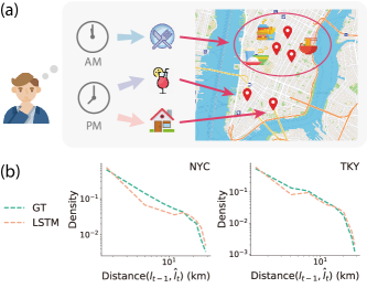
Figure 1. Illustrations for causality and spatial consistency in human mobility. (a) An example to explain the ”when$\rightarrow$what$\rightarrow$where” decision logic. (b) The deviation of the modeled displacement distribution via LSTM from the ground truth (GT) in New York City and Tokyo.

To this end, we propose a Causal and Spatial-constrained Long and Short-term Learner (CSLSL), a model integrating the decision logic and the consistency constraints of human mobility modeling. To model the ”when$\rightarrow$what$\rightarrow$where” decision logic, we introduce a causal structure in CSLSL. Based on a multi-task learning, the causal structure utilizes three similar network branches to model the regularities of time, activity, and location, respectively. In line with the ”when$\rightarrow$what$\rightarrow$where” logic, we explicitly build connections between the three branches in the causal structure. As for consistency, we exploratively propose a spatial-constrained loss to reduce the distance between the predicted and actual locations, and indirectly ensure the consistency of the spatial density distribution. In addition, we adopt a Long and Short-term Capturer (LSC) to learn the transition patterns of different time spans. There are two units in LSC that focus on long-term and short-term regularities respectively.

The main contributions of this work are summarized as follows:

• We propose CSLSL to integrate the travel decision logic and the macro-statistical consistency for human mobility modeling. To our best knowledge, CSLSL is the first model to learn the causality and consistency constraints for next location prediction.

• We introduce a causal structure that can capture not only the separate regularities of time, activity, and location, but also the ”when$\rightarrow$what$\rightarrow$where” causal dependencies. In this way, CSLSL models more essential travel logic in addition to sequence relationships.

• To ensure the consistency in spatial distribution, we propose a spatial-constrained loss to reduce the gap between the predicted and actual destinations.

• We evaluate CSLSL on three real-world datasets to confirm the performance improvements. We also conduct ablation studies and visualization analyses of results such as displacement distribution to demonstrate the effectiveness of our design.

2. Related Work

2.1. Next Location Prediction

Here we classify the approaches to the next location prediction problem into two categories: traditional and deep learning methods. Traditional methods mainly apply Markov chain (MC) and focus on constructing a better location transition probability matrix (Rendle et al., 2010; Cheng et al., 2013; Feng et al., 2015; Zhao et al., 2016). For instance, factorized personalized Markov chain (FPMC) combines the matrix factorization technique with Markov chains to learn users’ personalized transition matrices (Rendle et al., 2010). The limitation of the MC-based methods lies in the difficulty in capturing long-term and high-order regularity (Guo et al., 2020; Luo et al., 2021).

Deep learning methods have advantages of learning dense representation and complex dependency. Recently, RNN-based methods show promising performance in mining sequential information. A popular scheme of deep learning methods is incorporating time and distance intervals to assist the model in learning the spatio-temporal regularities of human mobility. Specifically, these methods integrate spatio-temporal information into hidden state transition (Liu et al., 2016), gate mechanisms (Kong and Wu, 2018; Manotumruksa et al., 2018; Zhao et al., 2019), or self-attention mechanisms (Lian et al., 2020; Luo et al., 2021), and exploit spatio-temporal contexts in a implicit manner. To leverage the spatio-temporal contexts, researchers explicitly used spatial and temporal factors as attention weights to select the historical hidden states (Yang et al., 2020; Zhao et al., 2020). Another scheme emphasizes the long-term patterns of human behavior, such as DeepMove (Feng et al., 2018) and LSTPM (Sun et al., 2020). They introduce two different components to model long-term and short-term preferences respectively. There is also another scheme that utilizes semantic information such as location categories to improve the performance of location prediction (Yu et al., 2020; Guo et al., 2020; Wang et al., 2021). However, methods that focus on modeling location transfer patterns in sequences cannot effectively capture complex human decision logic. In our work, we propose a causal structure to explicitly capture the ”when$\rightarrow$what$\rightarrow$where” decision logic.

2.2. Time- or Activity-jointed Location Prediction

The methods that jointly predict time or activity learn knowledge from related tasks to improve the prediction performance of location. RMTPP (Du et al., 2016) combines RNN and temporal point process (TPP) to jointly model the time and location information. He et al. (He et al., 2017) proposed a two-fold approach that predicts category with Bayesian Personalized Ranking (BPR) technique and then predicts the category-based location. Krishna et al. (Krishna et al., 2018) utilized two distinct LSTM networks to predict activities and durations. DeepJMT (Chen et al., 2020) fuses spatio-temporal information and social context to predict time and location with a hierarchical RNN and TPP technique. Sun et al. (Sun and Kim, 2021) proposed a hybrid LSTM and a sequential LSTM with a self-attention mechanism to jointly model location and travel time. The limitation of these approaches is that they attempt to implicitly and passively learn the correlation between time, category, and location information, but this relationship is explicit and can be directly exploited. In contrast, CSLSL explicitly models the causal dependencies between time, category, and location information through two structural designs.

2.3. Statistical Physics-informed human mobility modeling

Explicitly integrating knowledge of statistical physics contributes to guiding model optimization and improving the performance of machine learning methods. On the task of trajectory generation, researchers introduced knowledge of statistical physics to constrain the macroscopic performance of their models, such as the individual trajectory generation model TimeGeo (Jiang et al., 2016) and DITRAS (Pappalardo and Simini, 2018), and flow generation model DeepGravity (Simini et al., 2021). Unlike the trajectory generation task, only a limited amount of work on individual mobility prediction incorporates knowledge of statistical physics. Zhao et al. (Zhao et al., 2020) integrated domain knowledge, specifically a power-law decay for distances and an exponential decay for time intervals, into an attention mechanism to adjust the impact of historical information on current prediction. However, deep learning-based methods focus more on fitting individual behavior while neglecting group behavior constraints described by macro-statistical characteristics, for example, the regional attractiveness of city blocks. The spatial distribution of model prediction results should be consistent with the actual statistical distribution. Predicted locations closer to the actual location are more expected. Toward this, we propose a spatial-constrained loss function to narrow the distance between the predicted and actual locations, thereby ensuring the consistency of the spatial distribution.

3. Problem Formulation

A person’s travel behavior can be represented as a sequence of locations, associated with the timestamps and her user ID. In LBSN datasets, each location is also associated with its functional category to support the analysis of user’s activity. Let $\mathcal{U}=\{u_{1},\dots,u_{|\mathcal{U}|}\}$, $\mathcal{L}=\{l_{1},\dots,l_{|\mathcal{L}|}\}$ and $\mathcal{C}=\{c_{1},\dots,c_{|\mathcal{C}|}\}$ denote a set of users, locations and functional categories, respectively. Each location $l_{i}$ is associated with its category and geographical coordinate $(c_{i},lat_{i},lon_{i})$.

Definition 1 (Record). Record $r$ is a 3-tuple $(u_{i},l_{j},t_{k})$, representing that the user $u_{i}$ visited location $l_{j}$ at time $t_{k}$, where $u_{i}\in\mathcal{U},l_{j}\in\mathcal{L}$.

Definition 2 (Individual Trajectory). A person’s trajectory is defined as a record sequence $\mathcal{R}=\{r_{1},r_{2},\dots,r_{|\mathcal{R}|}\}$, which consists of the person’s all records arranged in chronological order. Note that the time interval between two consecutive records is heterogeneous due to the irregular travel behavior.

Definition 3 (Session). Session $S$ is a subsequence of records in a time slot. One user’s trajectory $\mathcal{R}$ can be split into a series of sessions with various strategies. For example, DeepMove adopts a specific time interval between two consecutive records to split the trajectory (Feng et al., 2018). Other strategies segment users’ trajectories using a fixed number of records (Yang et al., 2020; Luo et al., 2021) or a meaningful time window such as days, weeks, etc (Sun et al., 2020). We define the session where the prediction target is located as the short-term session $S_{p}$ and the previous historical sessions as long-term sessions $\{S_{q}\},q\in\{1,\dots,p-1\}$.

The location prediction problem is formulated as: given a record sequence of a user $\mathcal{R}_{t-1}=\{r_{1},\dots,r_{t-1}\}$, the goal is to predict where the user $u$ is most likely to go in her next trip. We use $\hat{l}_{t}$ to denote the predicted next location. Note that the timestamp of the next trip $t$ is also unknown.

4. Methodology

In this section, we first analyze the causality and consistency constraints in human mobility modeling, and then elaborately introduce the design of the proposed model, Casual and Spatial-constrained Long and Short-term Learner (CSLSL). The architecture of CSLSL is illustrated in Figure 2. It mainly consists of two parts, an embedding part for learning the representations of arrival time, category, and location, from users’ recent and historical records; and the second part for learning the regularities of mobility behavior in a multi-task learning based causal module and making predictions.

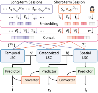
Figure 2. The architecture of the proposed CSLSL model.

4.1. Causality and Consistency Constraints

A common practice for next location prediction is to discover similar subsequences or location transition relationships from historical records. This is accomplished by integrating the context information such as distance or time intervals into attention or RNN-centered framework (Zhao et al., 2019; Yang et al., 2020; Sun et al., 2020; Luo et al., 2021). We can formulate such mainstream scheme as $P(\hat{l}_{t}|\mathcal{R}_{t-1})$, where $\mathcal{R}_{t-1}$ is the historical record sequence. Another scheme adopts multi-task learning techniques to jointly predict next location with time or activity (Chen et al., 2020; Sun and Kim, 2021), formulated as $P(\hat{l}_{t},\hat{c}_{t},\hat{t}|\mathcal{R}_{t-1})=P(\hat{l}_{t}|\mathcal{R}_{t-1})P(\hat{c}_{t}|\mathcal{R}_{t-1})P(\hat{t}|\mathcal{R}_{t-1})$, where we assume that the location category can approximate the type of activity. Although these two schemes combine contextual information to capture hidden regularities of location transition, they ignore the causal dependencies in the context information.

As aforementioned, we regard ”when”, ”what” and ”where” as three crucial elements to describe human mobility (Zhang et al., 2021; Pacheco et al., 2022). ”When” refers to the time the trip takes place, e.g. ”midday”. ”What” tells about the activities people participate in and also answers the reasons for the trip, such as ”having lunch”. ”Where” is the destination of the trip, like ”steakhouse”. Periodic activities exist in human mobility and occur at specific times and places, such as going to work in the morning and going to a restaurant for lunch, which reveals the correlation between the three elements. When we mention a specific timestamp, we have various activity choices. But we are accustomed to doing certain activities at certain times, such as going to the gym in the evening. Similarly, one activity (category) corresponds to multiple locations (POIs), while one location ID only corresponds to one activity, also reflected in the dataset. Moreover, our target is location prediction, thus location should be the final subtask to leverage the predicted time and activity information. Therefore, we summarize a ”when$\rightarrow$what$\rightarrow$where”, a.k.a. ”time$\rightarrow$activity$\rightarrow$location” causal relationship, which is in line with the coarse-to-fine logic of the human decision. The proposed scheme can be formulated as:

(1) $$P(\hat{l}_{t},\hat{c}_{t},\hat{t}|\mathcal{R}_{t-1})=P(\hat{l}_{t}|\hat{c}_{t},\hat{t},\mathcal{R}_{t-1})P(\hat{c}_{t}|\hat{t},\mathcal{R}_{t-1})P(\hat{t}|\mathcal{R}_{t-1}).$$

The scheme explicitly models the dependencies between time, activity, and location, and alleviates the difficulty of location prediction. For example, people are accustomed to going to restaurants at midday instead of bar, that is, $P(\hat{c}_{t}=restaurant|\hat{t}=midday,\mathcal{R}_{t-1})>P(\hat{c}_{t}=bar|\hat{t}=midday,\mathcal{R}_{t-1})$. Each individual has her personalized $P(\hat{l}_{t}|\hat{c}_{t}=restaurant,\hat{t}=midday,\mathcal{R}_{t-1})$, and the casual constrained location distribution is easier to learn than $P(\hat{l}_{t}|\mathcal{R}_{t-1})$. In CSLSL, we introduce a causal structure to implement the scheme. In experiments, we also demonstrate that ”time-¿acitivity-¿location” outperforms ”activity-¿time-¿location” and further discuss the reason.

On the other side, integrating physical knowledge provides more information and prior constraints to guide the optimization of deep learning models (Karniadakis et al., 2021; Willard et al., 2020). In human mobility modeling, one can expect that properly introducing the physical laws and domain knowledge would narrow down the gap between the output of deep learning-based approaches and the observed macro-statistical characteristics of human behavior. Due to the difficulty in applying statistical constraints in the training of deep learning models, here we consider the geographic spatial consistency in an indirect way. Specifically, we devise a loss function to constrain the distance between the predicted and actual locations. That is, the closer the predicted location is to the ground truth, the smaller loss we have. By this way, we can indirectly ensure the consistency of the displacement distribution and the consistency of the spatial distribution of travelers’ destinations.

4.2. Long and Short-term Capturer

Human travel behavior has long and short-cycle repetitive patterns, such as going to work every day and going to the supermarket once a week. Inspired by DeepMove (Feng et al., 2018) and LSTPM (Sun et al., 2020), we devise a Long and Short-term Capturer (LSC) to learn the behavioral patterns in different observation cycles. In the whole framework shown in Figure 2, we apply three LSCs to model the time, activity, and location sequences, respectively.

Let $\boldsymbol{e}^{l}\in\mathbb{R}^{d^{l}},\boldsymbol{e}^{c}\in\mathbb{R}^{d^{c}},\boldsymbol{e}^{t}\in\mathbb{R}^{d^{t}}$ and $\boldsymbol{e}^{u}\in\mathbb{R}^{d^{u}}$ denote the embedded representation of location, category, time and user, respectively. Given a historical record sequence $\mathcal{R}$, CSLSL embeds each record as $(\boldsymbol{e}^{l},\boldsymbol{e}^{c},\boldsymbol{e}^{t},\boldsymbol{e}^{u})$ in hidden spaces. Note that we first convert the continuous timestamp as the hour in a day $t^{h}$ and the day in a week $t^{d}$ to present the daily and weekly periodicity. By doing so, we have $\boldsymbol{e}^{t}=\boldsymbol{e}^{t^{h}}\oplus\boldsymbol{e}^{t^{d}}$. Then these representations in a record are concatenated together, $\boldsymbol{e}^{r}=\boldsymbol{e}^{l}\oplus\boldsymbol{e}^{c}\oplus\boldsymbol{e}^{t}\oplus\boldsymbol{e}^{u}$. We next split each user’s record sequence into multiple sessions with a certain time window, like days or weeks. The records in short-term session and long-term sessions are represented as $\widetilde{\boldsymbol{e}}^{r}_{p}=\{\boldsymbol{e}^{r}_{1},\dots,\boldsymbol{e}^{r}_{t-1}\}$ and $\{\widetilde{\boldsymbol{e}}^{r}_{q}\}=\{\widetilde{\boldsymbol{e}}^{r}_{1},\dots,\widetilde{\boldsymbol{e}}^{r}_{p-1}\}$, respectively.

Figure 3. The illustration of the LSC module.

Our proposed LSC consists of two capturers to learn the transition regularities in the short-term and long-term sessions, respectively, as shown in Figure 3. We formulate LSC as:

(2) $$\boldsymbol{h}_{t}=LSC(\widetilde{\boldsymbol{e}}^{r}_{p},\{\widetilde{\boldsymbol{e}}^{r}_{q}\},\boldsymbol{h}_{0}),$$

where $\boldsymbol{h}_{0}$ is the initial hidden state. In the LSC structure, the short-term capturer takes the hidden state $h_{|S_{p-1}|}$ of the long-term capturer as the initial hidden state to combine the historical information. Because GRU is simple but efficient in modeling temporal data, we apply a layer of GRU in both of the capturers:

(3) $$\boldsymbol{h}_{i}=GRU(\boldsymbol{e}^{r}_{i-1},\boldsymbol{h}_{i-1}),$$

where $i\in\{1,2,\dots,|S_{p-1}|\}$ for long-term capturer and $i\in\{1,2,\dots,t\}$ for short-term capturer.

4.3. Causal Structure

To model the ”time$\to$activity$\rightarrow$location” logic relationship discussed in subsection 4.1, we introduce a causal structure based on multi-task learning techniques. As illustrated in Figure 2, we utilize three branches with the same architecture to model the change patterns of time, activity, and location, respectively. Specifically, in each branch, we convey the same record representations to the LSC module and then transfer the output hidden states to the predictor. To explicitly model the summarized causal relation in human travel behavior, we next design two paths for information transfer between various tasks. The first path lies between two LSC modules, passing on the task-specific hidden states. The second path lies between two predictors. In this path, the predicted result of the upstream task is processed by the converter and then conveyed to the downstream task. Here we use the fully connected layer as the predictor (P) and converter(C). That is $\boldsymbol{y}=Linear(\boldsymbol{x})=\boldsymbol{W}\boldsymbol{x}+\boldsymbol{b}$.

Mathematically, the branch of ”time” is formulated as:

(4) $$\boldsymbol{h}^{t}_{t}=LSC(\widetilde{\boldsymbol{e}}^{r}_{p},\{\widetilde{\boldsymbol{e}}^{r}_{q}\},0),$$

(5) $$\hat{t}=Linear^{(P^{t})}(\boldsymbol{h}^{t}_{t}),$$

where $\boldsymbol{W}^{(P^{t})}\in\mathbb{R}^{1\times|\boldsymbol{h}^{t}|}$, $\boldsymbol{h}^{t}_{t}$ is the hidden state of the next time, and $\hat{t}$ is the predicted time. As the downstream task of ”time” in causal structure, the branch of ”activity” can be formulated as:

(6) $$\boldsymbol{h}^{c}_{t}=LSC(\widetilde{\boldsymbol{e}}^{r}_{p},\{\widetilde{\boldsymbol{e}}^{r}_{q}\},\boldsymbol{h}^{t}_{t}),$$

(7) $$\boldsymbol{c}_{t}=Linear^{(P^{c})}(\boldsymbol{h}^{c}_{t}\oplus Linear^{(C^{t})}(\hat{t})),$$

(8) $$\hat{c}_{t}=argmax(\boldsymbol{c}_{t}),$$

where $\boldsymbol{W}^{(C^{t})}\in\mathbb{R}^{|\boldsymbol{e}^{t}|\times 1},\boldsymbol{W}^{(P^{c})}\in\mathbb{R}^{|\mathcal{C}|\times(|\boldsymbol{h}^{c}|+|\boldsymbol{e}^{t}|)}$, $\boldsymbol{h}^{c}_{t}$ is the hidden state of the next activity, and $\hat{c}_{t}$ is the predicted activity. Eventually, we can formulate the branch of ”location” as:

(9) $$\boldsymbol{h}^{l}_{t}=LSC(\widetilde{\boldsymbol{e}}^{r}_{p},\{\widetilde{\boldsymbol{e}}^{r}_{q}\},\boldsymbol{h}^{c}_{t}),$$

(10) $$\boldsymbol{l}_{t}=Linear^{(P^{l})}(\boldsymbol{h}^{l}_{t}\oplus Linear^{(C^{c})}(\boldsymbol{c}_{t})),$$

(11) $$\hat{l}_{t}=argmax(\boldsymbol{l}_{t}),$$

where $\boldsymbol{W}^{(C^{c})}\in\mathbb{R}^{|\boldsymbol{e}^{c}|\times|\mathcal{C}|},\boldsymbol{W}^{(P^{l})}\in\mathbb{R}^{|\mathcal{L}|\times(|\boldsymbol{h}^{l}|+|\boldsymbol{e}^{c}|)}$, $\boldsymbol{h}^{l}_{t}$ is the hidden state of the next location, $\boldsymbol{l}_{t}$ is the distribution of predicted location, and $\hat{l}_{t}$ is the predicted location.

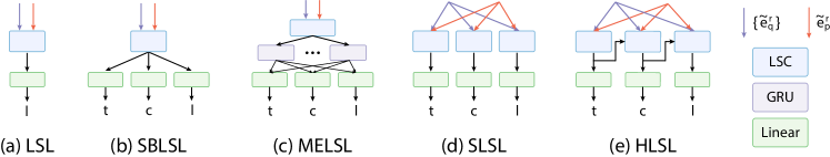
Figure 4. Structure variation. (a) Long and Short-term Learner (LSL); (b) Share-Bottom LSL (SBLSL); (c) Multi-Experts LSL (MELSL); (d) Separate LSL (SLSL); (e) Hierarchical LSL (HLSL). Note the gate networks of MELSL are not drawn for simplicity.

4.4. Spatial-constrained Loss Function

As discussed in subsection 4.1, for seeking an alignment of spatial distribution of destinations, we propose a spatial-constrained loss function to shorten the distance from the predicted location to the ground truth at individual level. The distance constraint can be regarded as a self-supervised auxiliary task, integrating the geographical information and restricting the candidate set for better next location prediction. The existing methods introduce the distance constraints in a regression subtask, directly predicting the geographical locations of destinations (Xue et al., 2021). However, in the classification scheme, we must query the coordinates of location IDs to calculate their distance. This operation is not derivable. We get inspiration from REINFORCE (Williams, 1992), which introduces the reward in the loss function to train a policy network, and also consider the distance error as a coefficient to weight the cross-entropy between ground truth and the predicted location ID with their physical distance. The spatial-constrained loss function is defined as:

(12) $$L_{s}=-\sum^{N}_{i=1}distance(\hat{l}_{t,i},l_{t,i})\cdot log(\sigma(\boldsymbol{l}_{t,j})),$$

where $N$ is the total number of records and $\sigma$ is the softmax function.

We next employ MAE loss for time prediction and cross entropy loss for category and location prediction. Thus we have $L_{t}=MAE(\hat{t},t)=\sum^{N}_{i=1}|\hat{t}_{i}-t_{i}|$ and $L_{*}=CrossEntropy(*)=-\sum^{N}_{i=1}log(\sigma(\boldsymbol{*_{t,i}})),*\in\{c,l\}$. Thus, the total loss function can be written as

(13) $$L_{total}=L_{l}+\lambda_{t}L_{t}+\lambda_{c}L_{c}+\lambda_{s}L_{s},$$

where $\lambda_{t},\lambda_{c},\lambda_{s}$ are weights for their loss functions.

4.5. Structure Comparison

There are various strategies for task combination in multi-task learning, such as share-bottom structure (Ruder, 2017; Qin et al., 2020), hierarchical structure (Sanh et al., 2019; Chen et al., 2020), and multi-expert structure (Ma et al., 2018; Qin et al., 2020). Inspired by these structures, we propose five variants, as shown in Figure 4, to demonstrate the advantages of our causal structure. Note that these variants use the same basic components as CSLSL, such as GRUs and fully connected layers.

Long and Short-term Learner (LSL) is a basic approach with only one branch to predict location. To jointly predict ”time”, ”activity”, and ”location”, Share-Bottom LSL (SBLSL) introduces two additional predictors that share the same bottom LSC module with the original one. Multi-Experts LSL (MELSL) is an advanced version of SBLSL, with a similar structure to Mixture of Sequential Expert (MoSE) (Qin et al., 2020). MELSL employs several GRUs as experts to focus on different aspects of sequence dependencies and gate networks to combine relevant aspects for each task.

Unlike the share-bottom structure, Separate LSL (SLSL) employs a separate branch for each task and the only shared information between each task is the same record representations. Considering the dependencies between tasks, Hierarchical LSL (HLSL) concatenates the record embedding and the output hidden state of the upstream task as the input of the downstream task. Thus the equation 3 changes to:

(14) $$\boldsymbol{h}^{k}_{i}=GRU(\boldsymbol{e}^{r}_{i-1}\oplus\boldsymbol{h}^{k-1}_{i},\boldsymbol{h}^{k}_{i-1}),$$

where $\boldsymbol{h}^{k}_{i}$ is the hidden state of the $k$-th task at $i$-th time step, and the equation 2 changes to:

(15) $$\boldsymbol{h}^{k}_{t}=LSC([\widetilde{\boldsymbol{e}}^{r}_{p},\widetilde{\boldsymbol{h}}^{k-1}_{p}],\{[\widetilde{\boldsymbol{e}}^{r}_{q},\widetilde{\boldsymbol{h}}^{k-1}_{q}]\},0),$$

where $[\widetilde{\boldsymbol{e}}^{r}_{p},\widetilde{\boldsymbol{h}}^{k-1}_{p}]=\{\boldsymbol{e}^{r}_{1}\oplus\boldsymbol{h}^{k-1}_{1},\dots,\boldsymbol{e}^{r}_{t-1}\oplus\boldsymbol{h}^{k-1}_{t-1}\}$.

5. Experiments

5.1. Data Description

We leverage three publicly available check-in datasets in the experiments: two datasets from Foursquare (Yang et al., 2014) in New York (NYC) and Tokyo (TKY) and one dataset from Gowalla (Cho et al., 2011) in Dallas. Data in NYC and TKY were collected from 3 April 2012 to 16 February 2013, and data in Dallas was collected from 4 October 2016 to 30 April 2017. The number of users, locations, records in three datasets are summarized in Table 1, where $|\mathcal{*}|$ denotes the number of $*$. The number of location categories $|\mathcal{C}|$ in NYC and TKY are 400 and 385, while Dallas does not contain category information.

To prepare data for baselines and proposed models, we first filter out both users and locations with fewer than 10 records, in line with previous work (Feng et al., 2018; Sun et al., 2020). We then merge the consecutive records with the same user and location on the same day. The statistic information of the raw and processed data are depicted in Table 1. After pre-processing, the number of categories for NYC and TKY are reduced to 308 and 286. For CSLSL and its variations, we split trajectories into sessions according to week due to the data sparsity. In addition, we require that each session contains at least two records and a user contains at least five sessions to guarantee a training/testing split of 8/2, following (Feng et al., 2018). All baselines have their own further data preparation strategies and the model-specific dataset information is also shown in Table 1. It’s noteworthy that, LSTPM (Sun et al., 2020) requires at least three records in each session and Flashback (Yang et al., 2020) limits the minimum records of each user to 100. These practices filter out more sparse data and reduce the challenge of prediction. Moreover, GETNext requires category information as input, thus it cannot work on dataset Dallas.

Table 1. Statistic information of raw and processed data.

	NYC			TKY			Dallas
	$|\mathcal{U}|$	$|\mathcal{L}|$	$|\mathcal{R}|$	$|\mathcal{U}|$	$|\mathcal{L}|$	$|\mathcal{R}|$	$|\mathcal{U}|$	$|\mathcal{L}|$	$|\mathcal{R}|$
Raw	1,083	38,333	227,428	2,293	61,858	573,703	5,894	5,767	167,016
Processed	1,083	4,638	139,183	2,293	7,222	427,746	2,412	5,642	146,117
FPMC-D	1,083	4,638	94,168	2,293	7,222	334,561	2,412	5,642	100,743
FPMC-W	1,083	4,638	92,260	2,293	7,222	303,854	2,412	5,642	122,419
DeepMove	1,061	4,627	111,968	2,284	7,206	333,215	1,193	5,346	93,911
Flashback	439	4,093	96,771	1,451	6,998	366,604	340	5,434	82,287
LSTPM	579	4,128	62,511	1,866	7,007	273,880	587	5,169	55,784
GeoSAN	1,073	4,611	138,229	2,289	7,209	427,157	2,300	5,357	142,980
STAN	1,000	4,503	82,783	2,200	7,047	201,831	2,400	5,615	95,656
GETNext	1,066	4,621	131,920	2,280	7,200	414,993	-	-	-
Ours	1,065	4,635	133,944	2,280	7,204	422,432	1,357	5,428	120,531

Table 2. Performance comparison between baselines, CSLSL, its variants and ablations on three real-world datasets.

	NYC						TKY						Dallas
	Category			Location			Category			Location			Location
	R@1	R@5	R@10	R@1	R@5	R@10	R@1	R@5	R@10	R@1	R@5	R@10	R@1	R@5	R@10
FPMC-D	0.217	0.510	0.631	0.173	0.424	0.526	0.462	0.623	0.688	0.176	0.408	0.503	0.086	0.204	0.261
FPMC-W	0.196	0.394	0.482	0.162	0.323	0.382	0.428	0.513	0.557	0.117	0.245	0.313	0.055	0.125	0.161
DeepMove	0.244	0.499	0.586	0.198	0.407	0.470	0.398	0.567	0.626	0.161	0.331	0.400	0.089	0.185	0.229
Flashback*	0.280	0.618	0.737	0.223	0.521	0.639	0.479	0.730	0.801	0.207	0.486	0.583	0.090	0.199	0.256
LSTPM*	0.335	0.659	0.765	0.267	0.560	0.662	0.461	0.727	0.797	0.231	0.457	0.543	0.123	0.247	0.316
GeoSAN	0.193	0.433	0.602	0.166	0.430	0.584	0.317	0.551	0.694	0.158	0.392	0.528	0.078	0.186	0.265
STAN	0.218	0.480	0.591	0.192	0.411	0.494	0.376	0.575	0.668	0.167	0.388	0.478	0.074	0.153	0.196
GETNext	0.303	0.646	0.749	0.246	0.536	0.622	0.452	0.758	0.844	0.216	0.456	0.550	-	-	-
LSL	0.288	0.587	0.684	0.242	0.506	0.589	0.446	0.697	0.762	0.225	0.462	0.548	0.101	0.203	0.254
SBLSL	0.290	0.595	0.682	0.242	0.488	0.571	0.446	0.769	0.851	0.229	0.460	0.545	0.107	0.194	0.234
MELSL	0.275	0.586	0.662	0.227	0.432	0.526	0.439	0.648	0.745	0.211	0.419	0.475	0.078	0.121	0.164
SLSL	0.281	0.611	0.722	0.253	0.534	0.632	0.409	0.731	0.825	0.233	0.458	0.559	0.114	0.220	0.272
HLSL	0.296	0.628	0.734	0.256	0.536	0.625	0.441	0.760	0.847	0.232	0.472	0.562	0.115	0.230	0.284
CLSL-ctl	0.315	0.647	0.745	0.257	0.543	0.636	0.472	0.780	0.861	0.227	0.472	0.560	-	-	-
CLSL	0.322	0.658	0.747	0.261	0.553	0.643	0.459	0.782	0.864	0.238	0.476	0.567	0.120	0.229	0.282
CSLSL-c	0.315	0.638	0.757	0.247	0.546	0.643	0.450	0.775	0.858	0.230	0.463	0.551	-	-	-
CSLSL-t	0.319	0.648	0.749	0.264	0.556	0.652	0.479	0.740	0.829	0.233	0.478	0.568	0.118	0.231	0.284
CSLSL	0.327	0.661	0.759	0.268	0.568	0.656	0.488	0.801	0.875	0.240	0.488	0.580	0.126	0.243	0.297

• Flashback and LSTPM filter out much more sparse users in their data preparation, reducing the challenge of prediction.

5.2. Baselines and Settings

Baselines. We compare CSLSL with the state-of-the-art baselines:

• FPMC (Rendle et al., 2010) is a Markov-based model that uses factorization to learn individual transition matrices.

• DeepMove (Feng et al., 2018) adopts an attention mechanism to learn long-term preference and an GRU module to capture short-term preference.

• Flashback (Yang et al., 2020) uses spatio-temporal distances as attention weights to search the historical hidden states for current prediction.

• LSTPM (Sun et al., 2020) considers temporal similarity and distance factor to model long-term preferences and geographical relevance to model short-term preferences.

• GeoSAN (Lian et al., 2020) designs a geography encoder to implicitly capture spatial proximity and introduces a loss function based on importance sampling to better use the informative negative samples.

• STAN (Luo et al., 2021) introduces a two-layer attention architecture with spatio-temporal relation matrices to explicitly capture the spatio-temporal correlations.

• GETNext (Yang et al., 2022) utilizes a GCN to integrate collective movement patterns and a transformer encoder to capture transition regularities. Besides, it introduces location categories as inputs and prediction targets.

Settings. For convincingly comparing these baselines with our CSLSL, we collected the open-source codes released by the authors and attempted to find the optimal hyper-parameters in the experiments. It’s worth noting that most of the baselines only predict next location, without category and time of visitation. Thus, we match the predicted location ID to its category for comparison and exclude the performance comparison of time prediction. Besides, we split users’ trajectories by day and week for FPMC model, referred to as FPMC-D and FPMC-W, respectively. For CSLSL, the dimensions of representation vectors $\boldsymbol{e}^{l},\boldsymbol{e}^{c},\boldsymbol{e}^{t^{h}},\boldsymbol{e}^{t^{d}}$ and $\boldsymbol{e}^{u}$ are set to 200, 100, 10, 20, and 20 for all datasets. The dimension of the hidden state in all GRUs is set to 600. We use the Adam optimizer with the learning rate of 0.0001, and $\lambda_{t}$, $\lambda_{c}$, and $\lambda_{s}$ are set to $10$.

Metrics. In the next location prediction task, what we care about is whether the actual location is in the top $N$ of our predictions, $N=\{1,5,10\}$. $Recall@N$ is the most commonly used metric and is equal to $Accuracy@N$ because we don’t have false positive (FP) and true negative (TN). The definition of $Recall@N$ is

(16) $$Recall@N=\frac{1}{|\mathcal{U}|}\sum_{u\in\mathcal{U}}\frac{|\mathcal{L}_{u}^{T}\cap\mathcal{L}_{u}^{P}|}{|\mathcal{L}_{u}^{T}|},$$

where $\mathcal{L}_{u}^{T}$ and $\mathcal{L}_{u}^{P}$ are the target and top $N$ prediction location sets, respectively.

5.3. Performance Comparison with Baselines

The experimental results are averaged over 10 independent runs and shown in Table 2. For each city, the results are presented in three pieces, representing the results of baselines (line 1-8), variants (line 9-14), and ablations (line 15-18), respectively. The best performance in each column is highlighted in bold text and the second best one is underlined. For NYC and TKY, we present the predicted results for categories and locations, while for Dallas, we only show the location prediction results due to the lack of category information.

From the experiment results, we can observe that the proposed CSLSL shows promising performances compared with baselines. In terms of $Recall@1$ in location prediction, CSLSL achieves $27\%$, $37\%$, and $43\%$ averaged performance improvements over these deep learning baselines in three datasets. For $Recall@1$ in category prediction, the improvements are $34\%$ and $23\%$ in NYC and TKY, respectively. Considering $Recall@\{5,10\}$ in location prediction, CSLSL achieves similar performances with LSTPM and Flashback, which filter more than $46\%,18\%,$ and $57\%$ of sparse users than we do on three datasets shown in Table 1. These similar performances in the more challenging dataset settings can also reflect the superiority of our model. Disregarding these two models, CSLSL still obtains over $20\%$ averaged improvements than the rest of deep learning baselines. Moreover, CSLSL has improved by 8.9% and 11.1% in Recall@1 in NYC and TKY compared to GetNext, which has similar dataset statistics to ours. The poor performances of all models on the Dallas dataset may be due to the data sparseness. Even so, CSLSL can still utilize the time-location relationship and the spatial constraints to achieve performance gains.

Among the baselines, we observe that the overall performance of location prediction on TKY is lower than NYC. This is probably because the TKY dataset has a larger number of users and locations than NYC, increasing the difficulty of mobility predicting. However, CSLSL obtains more performance improvement on TKY than NYC for location prediction compared with baselines. For instance, the performance of CSLSL improves 8.9% on NYC compared with GETNext, while the improvement is 11.1% on TKY. On the other side, the category predictions for all models have higher accuracy on TKY than on NYC. We may conclude that the larger performance improvement on TKY than NYC mainly owes to the proper modeling of the dependencies.

5.4. Performance Comparison with Variants

To fairly demonstrate the effectiveness of the proposed causal structure, here we develop an ablated version of CSLSL via dropping the spatial-constraint loss, namely CLSL, and compare it with the 5 variants discussed in the subsection 4.5. Moreover, we also consider the ”what$\to$when$\to$where” relationship, thus we change the order of these three branches in CLSL from ”time$\to$category$\to$location” to ”category$\to$time$\to$location” and this variant is named CLSL-ctl. We present the results of the variants and CLSL in the second and third pieces of Table 2. The category prediction results of LSL are obtained in the same way as the baselines.

Compared with LSL, SBLSL has a similar performance of location prediction and slightly improved performance of category prediction, suggesting that the shared bottom of SBLSL has indeed learned the category transfer regularities. However, these learned regularities make no contribution to the location prediction. Besides, the performance of MELSL is weaker than LSL and SBLSL, which may be because MELSL does not clarify the relationship between tasks and its experts cannot find suitable optimization directions. The better performance of SLSL than SBLSL indicates that the separate modules to learn transition relationships are better than the shared one. HLSL achieves the best performance in the second pieces of Table 2, suggesting that there are dependencies between time, category, and location, and that capturing the dependencies facilitates location prediction.

The performances of these variants are weaker than CLSL, suggesting that although these variants utilize temporal and categorical information, they cannot effectively and autonomously capture the dependencies between time, category, and location. In contrast, the causal structure explicitly captures the dependencies between tasks in two ways, thereby fully exploiting their dependencies to improve performance. Moreover, the better performance of CLSL than CLSL-ctl is in line with expectations, because location has stronger dependencies with category than time and category information can bring more performance gains for location prediction. Therefore, our proposed causal structure explicitly models ”time$\to$category$\to$location” rather than ”category$\to$time$\to$location”.

5.5. Ablation Study

We also conduct ablation studies to examine the contributions of different components in CSLSL. The ablated models include:

• LSL: the version that only keep the location branch.

• CLSL: the version that removes the spatial-constraint loss.

• CSLSL-t: the version that removes the time branch.

• CSLSL-c: the version that removes the category branch.

As shown in Table 2, we can find that CSLSL-t achieves better performance than CSLSL-c, indicating the ”category$\to$location” relationship has stronger dependency constraints than ”time$\to$location”. This result is also consistent with what we discussed in the subsection 5.4. The best performance of the complete CSLSL demonstrates the significance of the entire ”time$\to$category$\to$location” decision logic. Comparing the performance of CLSL and CSLSL, we can confirm that the spatial-constraint loss function have a positive impact on the performance improvement. Moreover, LSL achieves decent performance compared with baselines, probably because it leverages category information and the LSC module is capable of capturing the long-term and short-term preferences.

5.6. Results Visualization Analysis

We conduct result visualization analysis to further understand the effectiveness of the causal structure and the spatial-constrained loss. For the causal structure, we compare the category and the location prediction results of GETNext and CSLSL, as shown in Figure 5. We can observe that for CSLSL, the records with successfully predicted both categories and locations on NYC and TKY account for 21% and 20% of all records. Compared with GETNext, CSLSL successfully predicted 10% and 18% more locations with more accurately predicted categories on NYC and TKY, respectively. This intuitively indicates that the causal structure can enhance the location prediction with more accurate category prediction results. Interestingly, the location can be predicted correctly with an unsuccessfully predicted category. This is because the category information is introduced as additional auxiliary information without imposing mandatory constraints on the location prediction.

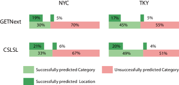
Figure 5. Effect analysis of the causal structure.

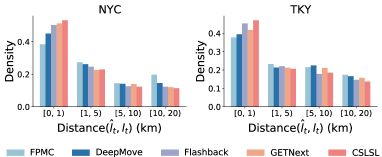
Figure 6. Distance distribution between the predicted and target location.

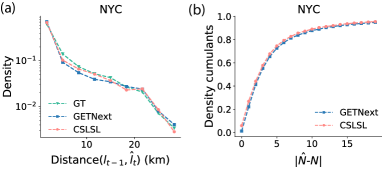
Figure 7. (a) Comparison of the predicted displacement with the ground truth (GT). (b) Prediction error comparison of regional attractiveness.

Regarding to the spatial-constrained loss, we examine whether the distances between predicted and actual locations are successfully constrained, and compare CSLSL with four baselines. As shown in Figure 6, the results show that the predicted locations of CSLSL is closer to the actual locations, which indicates that the proposed loss can successfully constrain the distance errors. Furthermore, we inspect the constraining effect of the proposed loss on spatial consistency. Figure 7(a) shows the comparison of the predicted displacement with the ground truth. It can be seen that the predicted displacement of CSLSL is closer to the true distribution. This is because the constraint between the predicted and actual locations can indirectly ensure the consistency of the predicted displacements and the ground truth. Figure 7(b) shows the prediction error of regional attractiveness. We divided the geographic regions into square grids with side length of 500m, and count the difference between the predicted and actual visits in each grid. As presented in Figure 7(b), CSLSL has a smaller prediction error of regional attractiveness, suggesting that the proposed loss successfully constrains the spatial consistency.

5.7. Sensitivity Analysis

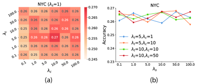
Figure 8. Analysis of parameter sensitivity.

We perform sensitivity analysis on dataset NYC to examine how the performance of CSLSL is affected by $\lambda_{*}$, $*\in\{t,c,s\}$. We first vary $\lambda_{t}$ and $\lambda_{c}$ to analyze the effect of time and category prediction subtasks with a fixed $\lambda_{s}=1$. Then we fix $\lambda_{t}$ and $\lambda_{c}$ and vary $\lambda_{s}$ to observe the impact of spatial-constrained auxiliary tasks. $Recall@1$ is chosen as the evaluation metric and the results of location prediction are averaged of three runs, shown in Figure 8.

From Figure 8 (a), we can observe that the performance of location prediction is more sensitive to $\lambda_{c}$ than $\lambda_{t}$, reflecting that the accurate category prediction exerts more influence on the location prediction accuracy, which is also consistent with our proposed decision logic. In addition, the best performance is obtained with $\lambda_{t}=5$ and $\lambda_{c}=10$ when $\lambda_{s}=1$. Figure 8 (b) shows that CSLSL reaches a more stable accuracy on NYC when $\lambda_{s}=5.0$, while the average accuracy is higher when $\lambda_{s}=10.0$. In summary, CSLSL is robust to these parameters and does not suffer from large performance fluctuations with parameter changes.

6. Conclusion

In this work, we propose a Causal and Spatial-constrained Long and Short-Term Learner (CSLSL) to incorporate the individual travel decision logic and the group consistency for next location prediction. In CSLSL, we introduce a causal structure based on multi-task learning to explicitly capture the ”when$\rightarrow$what$\rightarrow$where” decision logic and enhance location prediction by fully exploiting the temporal and categorized information. We further propose a simple but effective spatial-constrained loss function that acts as a self-supervised auxiliary task to incorporate geographical information and indirectly ensure spatial consistency. We conduct extensive experiments to confirm the effectiveness of the design. In the future, we will assess the scalability of CSLSL in dense mobility datasets with large number of users.

References

- (1)
- Arenas et al. (2020) Alex Arenas, Wesley Cota, Jesús Gómez-Gardeñes, Sergio Gómez, Clara Granell, Joan T Matamalas, David Soriano-Paños, and Benjamin Steinegger. 2020. Modeling the spatiotemporal epidemic spreading of COVID-19 and the impact of mobility and social distancing interventions. Physical Review X 10, 4 (2020), 041055.
- Barbosa et al. (2018) Hugo Barbosa, Marc Barthelemy, Gourab Ghoshal, Charlotte R James, Maxime Lenormand, Thomas Louail, Ronaldo Menezes, José J Ramasco, Filippo Simini, and Marcello Tomasini. 2018. Human mobility: Models and applications. Physics Reports 734 (2018), 1–74.
- Chen et al. (2020) Yile Chen, Cheng Long, Gao Cong, and Chenliang Li. 2020. Context-aware deep model for joint mobility and time prediction. In Proceedings of the 13th International Conference on Web Search and Data Mining. 106–114.
- Cheng et al. (2013) Chen Cheng, Haiqin Yang, Michael R Lyu, and Irwin King. 2013. Where you like to go next: Successive point-of-interest recommendation. In Twenty-Third international joint conference on Artificial Intelligence.
- Cho et al. (2011) Eunjoon Cho, Seth A Myers, and Jure Leskovec. 2011. Friendship and mobility: user movement in location-based social networks. In Proceedings of the 17th ACM SIGKDD international conference on Knowledge discovery and data mining. 1082–1090.
- Çolak et al. (2016) Serdar Çolak, Antonio Lima, and Marta C González. 2016. Understanding congested travel in urban areas. Nature communications 7, 1 (2016), 1–8.
- Du et al. (2016) Nan Du, Hanjun Dai, Rakshit Trivedi, Utkarsh Upadhyay, Manuel Gomez-Rodriguez, and Le Song. 2016. Recurrent marked temporal point processes: Embedding event history to vector. In Proceedings of the 22nd ACM SIGKDD international conference on knowledge discovery and data mining. 1555–1564.
- Feng et al. (2018) Jie Feng, Yong Li, Chao Zhang, Funing Sun, Fanchao Meng, Ang Guo, and Depeng Jin. 2018. Deepmove: Predicting human mobility with attentional recurrent networks. In Proceedings of the 2018 world wide web conference. 1459–1468.
- Feng et al. (2015) Shanshan Feng, Xutao Li, Yifeng Zeng, Gao Cong, Yeow Meng Chee, and Quan Yuan. 2015. Personalized ranking metric embedding for next new poi recommendation. In Twenty-Fourth International Joint Conference on Artificial Intelligence.
- Gonzalez et al. (2008) Marta C Gonzalez, Cesar A Hidalgo, and Albert-Laszlo Barabasi. 2008. Understanding individual human mobility patterns. nature 453, 7196 (2008), 779–782.
- Guo et al. (2020) Qing Guo, Zhu Sun, Jie Zhang, and Yin-Leng Theng. 2020. An attentional recurrent neural network for personalized next location recommendation. In Proceedings of the AAAI Conference on artificial intelligence, Vol. 34. 83–90.
- He et al. (2017) Jing He, Xin Li, and Lejian Liao. 2017. Category-aware Next Point-of-Interest Recommendation via Listwise Bayesian Personalized Ranking.. In IJCAI, Vol. 17. 1837–1843.
- He et al. (2016) Jing He, Xin Li, Lejian Liao, Dandan Song, and William Cheung. 2016. Inferring a personalized next point-of-interest recommendation model with latent behavior patterns. In Proceedings of the AAAI Conference on Artificial Intelligence, Vol. 30.
- Jia et al. (2020) Jayson S Jia, Xin Lu, Yun Yuan, Ge Xu, Jianmin Jia, and Nicholas A Christakis. 2020. Population flow drives spatio-temporal distribution of COVID-19 in China. Nature 582, 7812 (2020), 389–394.
- Jiang et al. (2016) Shan Jiang, Yingxiang Yang, Siddharth Gupta, Daniele Veneziano, Shounak Athavale, and Marta C González. 2016. The TimeGeo modeling framework for urban mobility without travel surveys. Proceedings of the National Academy of Sciences 113, 37 (2016), E5370–E5378.
- Karniadakis et al. (2021) George Em Karniadakis, Ioannis G Kevrekidis, Lu Lu, Paris Perdikaris, Sifan Wang, and Liu Yang. 2021. Physics-informed machine learning. Nature Reviews Physics 3, 6 (2021), 422–440.
- Kong and Wu (2018) Dejiang Kong and Fei Wu. 2018. HST-LSTM: A Hierarchical Spatial-Temporal Long-Short Term Memory Network for Location Prediction.. In IJCAI, Vol. 18. 2341–2347.
- Krishna et al. (2018) Kundan Krishna, Deepali Jain, Sanket V Mehta, and Sunav Choudhary. 2018. An lstm based system for prediction of human activities with durations. Proceedings of the ACM on Interactive, Mobile, Wearable and Ubiquitous Technologies 1, 4 (2018), 1–31.
- Lian et al. (2020) Defu Lian, Yongji Wu, Yong Ge, Xing Xie, and Enhong Chen. 2020. Geography-aware sequential location recommendation. In Proceedings of the 26th ACM SIGKDD international conference on knowledge discovery & data mining. 2009–2019.
- Liu et al. (2016) Qiang Liu, Shu Wu, Liang Wang, and Tieniu Tan. 2016. Predicting the next location: A recurrent model with spatial and temporal contexts. In Thirtieth AAAI conference on artificial intelligence.
- Luca et al. (2020) Massimiliano Luca, Gianni Barlacchi, Bruno Lepri, and Luca Pappalardo. 2020. Deep learning for human mobility: a survey on data and models. arXiv preprint arXiv:2012.02825 (2020).
- Luo et al. (2021) Yingtao Luo, Qiang Liu, and Zhaocheng Liu. 2021. STAN: Spatio-Temporal Attention Network for Next Location Recommendation. In Proceedings of the Web Conference 2021. 2177–2185.
- Ma et al. (2018) Jiaqi Ma, Zhe Zhao, Xinyang Yi, Jilin Chen, Lichan Hong, and Ed H Chi. 2018. Modeling task relationships in multi-task learning with multi-gate mixture-of-experts. In Proceedings of the 24th ACM SIGKDD International Conference on Knowledge Discovery & Data Mining. 1930–1939.
- Manotumruksa et al. (2018) Jarana Manotumruksa, Craig Macdonald, and Iadh Ounis. 2018. A contextual attention recurrent architecture for context-aware venue recommendation. In The 41st International ACM SIGIR Conference on Research & Development in Information Retrieval. 555–564.
- Pacheco et al. (2022) Diogo Pacheco, Marcos Oliveira, Zexun Chen, Hugo Barbosa, Brooke Foucault-Welles, Gourab Ghoshal, and Ronaldo Menezes. 2022. Predictability states in human mobility. arXiv preprint arXiv:2201.01376 (2022).
- Pappalardo and Simini (2018) Luca Pappalardo and Filippo Simini. 2018. Data-driven generation of spatio-temporal routines in human mobility. Data Mining and Knowledge Discovery 32, 3 (2018), 787–829.
- Qin et al. (2020) Zhen Qin, Yicheng Cheng, Zhe Zhao, Zhe Chen, Donald Metzler, and Jingzheng Qin. 2020. Multitask mixture of sequential experts for user activity streams. In Proceedings of the 26th ACM SIGKDD International Conference on Knowledge Discovery & Data Mining. 3083–3091.
- Rendle et al. (2010) Steffen Rendle, Christoph Freudenthaler, and Lars Schmidt-Thieme. 2010. Factorizing personalized markov chains for next-basket recommendation. In Proceedings of the 19th international conference on World wide web. 811–820.
- Ruder (2017) Sebastian Ruder. 2017. An overview of multi-task learning in deep neural networks. arXiv preprint arXiv:1706.05098 (2017).
- Sanh et al. (2019) Victor Sanh, Thomas Wolf, and Sebastian Ruder. 2019. A hierarchical multi-task approach for learning embeddings from semantic tasks. In Proceedings of the AAAI Conference on Artificial Intelligence, Vol. 33. 6949–6956.
- Simini et al. (2021) Filippo Simini, Gianni Barlacchi, Massimilano Luca, and Luca Pappalardo. 2021. A Deep Gravity model for mobility flows generation. Nature communications 12, 1 (2021), 1–13.
- Song et al. (2010) Chaoming Song, Zehui Qu, Nicholas Blumm, and Albert-László Barabási. 2010. Limits of predictability in human mobility. Science 327, 5968 (2010), 1018–1021.
- Sun and Kim (2021) Jie Sun and Jiwon Kim. 2021. Joint prediction of next location and travel time from urban vehicle trajectories using long short-term memory neural networks. Transportation Research Part C: Emerging Technologies 128 (2021), 103114.
- Sun et al. (2020) Ke Sun, Tieyun Qian, Tong Chen, Yile Liang, Quoc Viet Hung Nguyen, and Hongzhi Yin. 2020. Where to go next: Modeling long-and short-term user preferences for point-of-interest recommendation. In Proceedings of the AAAI Conference on Artificial Intelligence, Vol. 34. 214–221.
- Wang et al. (2021) Huandong Wang, Qiaohong Yu, Yu Liu, Depeng Jin, and Yong Li. 2021. Spatio-Temporal Urban Knowledge Graph Enabled Mobility Prediction. Proceedings of the ACM on Interactive, Mobile, Wearable and Ubiquitous Technologies 5, 4 (2021), 1–24.
- Willard et al. (2020) Jared Willard, Xiaowei Jia, Shaoming Xu, Michael Steinbach, and Vipin Kumar. 2020. Integrating physics-based modeling with machine learning: A survey. arXiv preprint arXiv:2003.04919 1, 1 (2020), 1–34.
- Williams (1992) Ronald J Williams. 1992. Simple statistical gradient-following algorithms for connectionist reinforcement learning. Reinforcement learning (1992), 5–32.
- Xu et al. (2021) Fengli Xu, Yong Li, Depeng Jin, Jianhua Lu, and Chaoming Song. 2021. Emergence of urban growth patterns from human mobility behavior. Nature Computational Science 1, 12 (2021), 791–800.
- Xu et al. (2018) Yanyan Xu, Serdar Çolak, Emre C Kara, Scott J Moura, and Marta C González. 2018. Planning for electric vehicle needs by coupling charging profiles with urban mobility. Nature Energy 3, 6 (2018), 484–493.
- Xu et al. (2019) Yanyan Xu, Shan Jiang, Ruiqi Li, Jiang Zhang, Jinhua Zhao, Sofiane Abbar, and Marta C González. 2019. Unraveling environmental justice in ambient PM2. 5 exposure in Beijing: A big data approach. Computers, Environment and Urban Systems 75 (2019), 12–21.
- Xue et al. (2021) Hao Xue, Flora Salim, Yongli Ren, and Nuria Oliver. 2021. MobTCast: Leveraging auxiliary trajectory forecasting for human mobility prediction. Advances in Neural Information Processing Systems 34 (2021), 30380–30391.
- Yang et al. (2020) Dingqi Yang, Benjamin Fankhauser, Paolo Rosso, and Philippe Cudre-Mauroux. 2020. Location Prediction over Sparse User Mobility Traces Using RNNs: Flashback in Hidden States!. In Proceedings of the Twenty-Ninth International Joint Conference on Artificial Intelligence. 2184–2190.
- Yang et al. (2014) Dingqi Yang, Daqing Zhang, Vincent W Zheng, and Zhiyong Yu. 2014. Modeling user activity preference by leveraging user spatial temporal characteristics in LBSNs. IEEE Transactions on Systems, Man, and Cybernetics: Systems 45, 1 (2014), 129–142.
- Yang et al. (2022) Song Yang, Jiamou Liu, and Kaiqi Zhao. 2022. GETNext: Trajectory Flow Map Enhanced Transformer for Next POI Recommendation. In SIGIR.
- Yu et al. (2020) Fuqiang Yu, Lizhen Cui, Wei Guo, Xudong Lu, Qingzhong Li, and Hua Lu. 2020. A category-aware deep model for successive poi recommendation on sparse check-in data. In Proceedings of the web conference 2020. 1264–1274.
- Zhang et al. (2021) Wanyi Zhang, Qiang Shen, Stefano Teso, Bruno Lepri, Andrea Passerini, Ivano Bison, and Fausto Giunchiglia. 2021. Putting human behavior predictability in context. EPJ Data Science 10, 1 (2021), 42.
- Zhao et al. (2020) Kangzhi Zhao, Yong Zhang, Hongzhi Yin, Jin Wang, Kai Zheng, Xiaofang Zhou, and Chunxiao Xing. 2020. Discovering Subsequence Patterns for Next POI Recommendation.. In IJCAI. 3216–3222.
- Zhao et al. (2019) Pengpeng Zhao, Haifeng Zhu, Yanchi Liu, Jiajie Xu, Zhixu Li, Fuzhen Zhuang, Victor S Sheng, and Xiaofang Zhou. 2019. Where to Go Next: A Spatio-Temporal Gated Network for Next POI Recommendation. In Proceedings of the AAAI Conference on Artificial Intelligence, Vol. 33. 5877–5884.
- Zhao et al. (2016) Shenglin Zhao, Tong Zhao, Haiqin Yang, Michael R Lyu, and Irwin King. 2016. STELLAR: Spatial-temporal latent ranking for successive point-of-interest recommendation. In Thirtieth AAAI conference on artificial intelligence.