Gaia Data Release 3
$G_{\rm RVS}$ photometry from the RVS spectra

Abstract

Context. Gaia Data Release 3 (DR3) contains the first release of magnitudes estimated from the integration of Radial Velocity Spectrometer (RVS) spectra for a sample of about 32.2 million stars brighter than $G_{\rm RVS}\sim 14$ mag (or $G\sim 15$ mag).

Aims. In this paper, we describe the data used and the approach adopted to derive and validate the $G_{\rm RVS}$  magnitudes published in DR3. We also provide estimates of the $G_{\rm RVS}$ passband and associated $G_{\rm RVS}$ zero-point.

Methods. We derived $G_{\rm RVS}$ photometry from the integration of RVS spectra over the wavelength range from 846 to 870 nm. We processed these spectra following a procedure similar to that used for DR2, but incorporating several improvements that allow a better estimation of $G_{\rm RVS}$. These improvements pertain to the stray-light background estimation, the line spread function calibration, and the detection of spectra contaminated by nearby relatively bright sources. We calibrated the $G_{\rm RVS}$ zero-point every 30 hours based on the reference magnitudes of constant stars from the Hipparcos catalogue, and used them to transform the integrated flux of the cleaned and calibrated spectra into epoch magnitudes. The $G_{\rm RVS}$ magnitude of a star published in DR3 is the median of the epoch magnitudes for that star. We estimated the $G_{\rm RVS}$ passband by comparing the RVS spectra of 108 bright stars with their flux-calibrated spectra from external spectrophotometric libraries.

Results. The $G_{\rm RVS}$  magnitude provides information that is complementary to that obtained from the $G$, $G_{\rm BP}$, and $G_{\rm RP}$ magnitudes, which is useful for constraining stellar metallicity and interstellar extinction. The median precision of $G_{\rm RVS}$ measurements ranges from about 0.006 mag for the brighter stars (i.e. with $3.5\mathrel{\hbox to0.0pt{\lower 3.5pt\hbox{$\mathchar 536\relax$}\hss}\raise 1.5pt\hbox{$\mathchar 316\relax$}}G_{\rm RVS}\mathrel{\hbox to0.0pt{\lower 3.5pt\hbox{$\mathchar 536\relax$}\hss}\raise 1.5pt\hbox{$\mathchar 316\relax$}}6.5$ mag) to 0.125 mag at the faint end. The derived $G_{\rm RVS}$ passband shows that the effective transmittance of the RVS is approximately 1.23 times better than the pre-launch estimate.

1 Introduction

The high-resolution spectra collected by the Radial Velocity Spectrometer (RVS) on board Gaia (Gaia Collaboration et al., 2016) offer the possibility to define a narrow-band Vega-system $G_{\rm RVS}$ magnitude linked to the effective spectral transmittance of the instrument. Gaia Data Release 3 (DR3, Gaia Collaboration et al., 2022) contains the first release of $G_{\rm RVS}$ magnitudes estimated by the RVS pipeline using the flux integrated in the RVS spectra. These magnitudes are provided for about 32.2 million bright stars observed by Gaia, along with the $G$, $G_{\rm BP}$, and $G_{\rm RP}$ magnitudes obtained from the astrometric images, and the blue and red photometers, respectively (Riello et al., 2021).

The $G_{\rm RVS}$ measurements are published in the Gaia archive gaia_source table in the column labelled grvs_mag. The associated uncertainties are listed in the column grvs_mag_error and the number of epoch measurements used to obtain grvs_mag in the column grvs_mag_nbtransits. In the following, we refer to these quantities using their Gaia archive name, while we use the term $G_{\mathrm{RVS}}^{\rm{ext}}$ to designate $G_{\rm RVS}$ magnitudes obtained from external, that is non-RVS, data (including rough estimates by the onboard software, $G_{\mathrm{RVS}}^{\rm{onboard}}$, and finer estimates from the ground processing of Gaia astrometric images and red-photometer spectra).

The RVS was designed and optimised to obtain the spectra of the brightest stars observed by Gaia (i.e. brighter than the RVS magnitude limit of $G_{\mathrm{RVS}}^{\rm{onboard}}\sim 16.2$ mag). The primary goal of the RVS pipeline is to measure the all-epoch-combined radial velocities of these stars, with the measurement of grvs_mag being a secondary task. Each intermediate data release allows us to progress on these tasks, because the processing of more epoch data implies a higher signal-to-noise ratio (S/N) of the combined RVS spectra and the possibility to reach fainter magnitudes. In DR3, radial velocities are provided down to ${\tt grvs\_mag}\sim 14$ mag, compared to only $\sim 12$ mag in DR2. We aim to approach the RVS magnitude limit of $\sim 16$ in Gaia Data Release 4 (DR4).

This paper, focused on grvs_mag, is part of a series of papers dedicated to specific products of the RVS pipeline: the mean radial velocities are described in Katz et al. (2022) and, for hot stars, in Blomme et al. (2022); the double-lined radial velocities in Damerdji & et al. (2022); the mean projected rotational velocities in Fremat et al. (2022); and the mean spectra in Seabroke & et al. (2022).

In this paper, we describe the reduction process and method used to convert the raw RVS spectra into the grvs_mag magnitudes published in DR3. The paper is organised as follows. In Sect. 2, we present the RVS data used. The processing of the RVS spectra and the estimation of grvs_mag from these spectra are described in Sects. 3 and 4, respectively. Section 5 presents an alternative estimation of $G_{\rm RVS}$ based on the $G$ and $G_{\rm RP}$ magnitudes. In Sect. 6, we describe the validation of grvs_mag and the performances achieved, while in Sect. 7, we compute and provide the $G_{\rm RVS}$ passband. Section 8 illustrates the potential of grvs_mag to constrain interstellar extinction and stellar metallicity and to separate cool dwarfs from cool giants. Our conclusions are summarised in Sect. 9.

2 The data used

2.1 The RVS spectra

We refer to Cropper et al. (2018) and Sartoretti et al. (2018) for a complete description of the acquisition and processing of the RVS spectra. Briefly, as Gaia continuously scans the sky, stars brighter than $G_{\mathrm{RVS}}^{\rm{onboard}}=16.2$ mag transiting through one of the four rows splitting the RVS focal plane in the across-scan (AC) direction will have their spectrum recorded in each of the three CCDs along that row (see figure 1 of Sartoretti et al., 2018), so long as the onboard limit to the number of spectra that can be obtained simultaneously is not reached (Cropper et al., 2018). This limit is set by the maximum number of 72 samples that can be read by the serial register (in the AC direction) and corresponds to a maximum density of 35 000 sources/deg². When this limit is reached, priority is given to the brighter sources.

In the RVS spectra, starlight is dispersed over about 1100 pixels in the along-scan (AL) direction, sampling the wavelength range from 845 to 872 nm with a resolving power of $R\approx 11,500$ (resolution element of about 3 pixels). The wings of the spectra are excluded during processing, reducing the effective length of the spectra to [846; 870] as illustrated in Fig. 1.

The exposure time on each of the three CCDs along a row of the RVS focal plane is fixed at 4.4 seconds by the scanning requirements, resulting in low S/Ns in the spectra of the fainter stars. As an example, the typical S/N per sample in the spectrum of a faint source with grvs_mag$\,\sim 14$ recorded by one of the RVS CCDs for nominal stray-light level (70 e-/sample) is only $\sim$0.7.

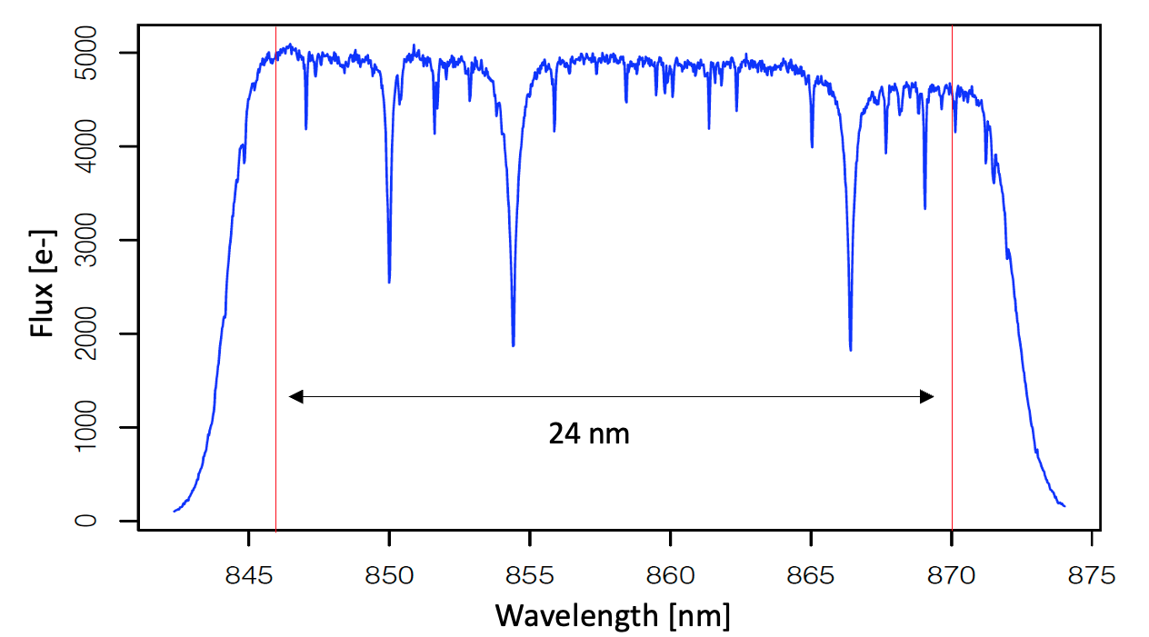
Figure 1: $G_{\rm RVS}$ bandwidth (delimited by the two vertical orange lines) extending over 24 nm from 846 to 870 nm. The fluxes of the available RVS epoch spectra of a source are integrated between these two wavelengths to estimate the magnitude grvs_mag, following the procedure outlined in Sects. 3 and 4. The Ca II triplet (at 850.035, 854.444, and 866.452 nm; rest-wavelengths in vacuum), prominent in the spectra of medium-temperature, FGK-, and late M-type stars, is the dominant feature found in the majority of RVS stellar spectra. The epoch CCD spectrum shown is that of a solar-type star with ${\tt grvs\_mag}=4.680\pm 0.045$ mag.

2.2 Time gaps in the data

The spectra processed by the DR3 pipeline were acquired by the RVS between onboard mission timeline (OBMT) 1078.3795 (25 July 2014) and OBMT 5230.0880 (28 May 2017). The OBMT, generated by the Gaia onboard clock, counts the number of six-hour spacecraft revolutions since launch. The relation to convert OBMT into barycentric coordinate time (TCB) is provided by Eq. 1 of Gaia Collaboration et al. (2021). All events on board are given in OBMT.

This 34-months time interval contains gaps over which the collected data were of poor quality and could not be used by the RVS pipeline. These gaps, when added together, cover 7.8% of the total observing time and were mostly caused by spacecraft events. The largest gaps were caused by three decontamination campaigns starting at OBMT 1317, 2330, and 4112.8, each requiring about 70 revolutions for the satellite to reach thermal equilibrium again. The start and end times of the gaps used by the RVS pipeline are available from the cosmos pages.

2.3 Source selection: $G_{\mathrm{RVS}}^{\rm{ext}}\leq 14$

grvs_mag cannot be used to preselect sources to be processed by the RVS pipeline because it is a final product of this pipeline. A $G_{\mathrm{RVS}}^{\rm{ext}}$ magnitude, measured from non-RVS data (Sect. 1), must be used instead.

Neither the $G$ magnitude (measured from the Gaia astrometric images) nor the $G_{\rm RP}$ magnitude (measured from the red-photometer data) published in Gaia-EDR3 (Gaia Collaboration et al., 2021) were available at the time the DR3 RVS processing started. Thus, estimates of these quantities from DR2 data were adopted instead to compute $G_{\mathrm{RVS}}^{\rm{ext}}$ using the transformation formulae in Eqs. (2) and (3) of Gaia Collaboration et al. (2018b). This could not be achieved for new sources observed since DR2 or sources for which the source identifier had changed. For such sources, the onboard magnitude $G_{\mathrm{RVS}}^{\rm{onboard}}$ was used to estimate $G_{\mathrm{RVS}}^{\rm{ext}}$. These sources represent about 2.6% of our final sample.

The sources with $G_{\mathrm{RVS}}^{\rm{ext}}\leq 14$ from this sample represent about 20% of the spectra observed by the RVS over the period of interest (Sect. 2.2). The selection on the basis of $G_{\mathrm{RVS}}^{\rm{ext}}$ also implies that some sources making the magnitude cut can end up with a grvs_mag measurements of fainter than 14 mag. Measurements of grvs_mag of fainter than 14.1 mag were considered spurious, mostly affected by inaccurate background estimation, and have not been published (see Sect. 6.2).

2.4 Spectrum selection

For the purpose of grvs_mag estimation, only the clean spectra are selected. To limit the contamination from nearby sources, the spectra presenting a truncated window (i.e. for which the spectrum window on the CCD overlaps with that of a nearby source) are excluded (some of these spectra are still used for the radial velocity estimation, after having been deblended; see Seabroke et al. 2021 and Seabroke & et al. 2022).

Other spectra excluded during the processing (see Sect. 3) are: the spectra with non-truncated window, but still potentially contaminated by nearby relatively bright sources; the spectra acquired over bad pixels or in a region with overly high levels of stray light; those with a negative total flux after bias and background subtraction; and those with too many samples saturated or affected by cosmic rays. In the end, of the 2.8 billion spectra with $G_{\mathrm{RVS}}^{\rm{ext}}\leq 14$ treated by the DR3 RVS pipeline (100 times more spectra than for DR2), about 1.5 billion are retained to estimate grvs_mag.

3 Processing of RVS spectra

The updated DR3 pipeline is described in the online documentation (Sartoretti et al., 2022), and the algorithms for performing the cleaning and calibration of the RVS spectra are described in detail in Sartoretti et al. (2018, Sects 5 and 6). In this section, we summarise the processing steps relevant to the computation of grvs_mag. We also describe in some detail new functionalities of the pipeline that allowed improvements in the estimation of grvs_mag, such as stray-light background estimation and the identification of spectra contaminated by neighbouring spectra.

3.1 The processing steps

Each individual RVS CCD spectrum passes through the following processing steps relevant to grvs_mag estimation. The aim is to compute TotFlux, the star flux integrated from the RVS spectrum.

1. The flux in the raw spectrum, in Analog Digital Units (ADU), is corrected for electronic bias and non-uniform offset (Hambly et al., 2018).

2. All pixels with fluxes exceeding $\sim$ 50 000 ADU are flagged as ‘saturated’. In practice, such pixels are assigned the numerical-saturation value of 65 535 ADU, as shown in Fig. 2. This procedure flags by default all pixels reaching physical saturation, because the average full-well capacity of an RVS CCD pixel is 190 000 e^-, corresponding to 336 300 ADU (see Table 1 of Hambly et al., 2018). Spectra presenting saturated pixels are not used for the $G_{\rm RVS}$ zero-point estimation (Sect. 4.1), while a maximum of 40 saturated pixels are allowed for the estimation of the $G^{\rm{epoch}}_{\mathrm{RVS}}$ epoch magnitude (Sect. 4.2).

3. The flux is transformed into photoelectrons using the on-ground-measured CCD gain values (0.53 e^- ADU^-1).

4. The stray-light background is subtracted from the spectrum (see Sect. 3.2 for more details). The spectra with negative total flux caused by over-subtraction of the background are removed from the pipeline, which induces a systematic overestimate of the flux of faint stars (see Sect. 6.1). Also removed are the spectra for which the background is too high (i.e. higher than 100 e^- pixel^-1 s^-1; or higher than 40 e^- pixel^-1 s^-1 with an uncertainty higher than 0.4 e^- pixel^-1 s^-1).

5. The flux loss outside the spectrum window on the CCD is estimated using the model of line spread function in the AC direction (LSF-AC) obtained in the pipeline. The LSF-AC calibration is a new functionality of the DR3 pipeline and is described in the online documentation (Sartoretti et al., 2022, Sect. 6.3.4). The LSF-AC profile is measured over an AC pixel range of $\pm(5+2.5)$ pixels from the centre (i.e. out to 2.5 pixels on each side beyond the 10-pixel-wide window in the AC direction). Outside of this range, the AC LSF is extrapolated to zero at $\pm$20 pixels. The flux loss outside the window is estimated using the extrapolated LSF-AC profile (i.e. over 15 pixels, or 2.67^′′, on each side of the nominal window) and is typically of the order of 5%.

6. Spectra containing any column from the cosmetic-defect list (see the online documentation: Sartoretti et al. 2022, table 6.2) are flagged and removed from the pipeline.

7. Spectra contaminated by a nearby source are flagged and removed from the pipeline (see Sect. 3.3 below for a description of the detection of contaminants).

8. Cosmic rays are removed. If the number of pixels affected by cosmic rays reaches 100, the spectrum is removed from the pipeline.

9. 2D windows (pertaining to stars with $G_{\mathrm{RVS}}^{\rm{onboard}}\leq 7$; see figure 1 of Sartoretti et al., 2018) are optimally collapsed (Horne, 1986) into 1D spectra if there are no saturated pixels. Otherwise, the 2D windows are collapsed into 1D spectra with a simple summing in the AC direction.

10. The wavelength calibration is applied, and the wavelength range is cut to 846–870 nm to remove the wings of the RVS spectrum (Fig. 1). This is the widest possible (integer) wavelength range properly sampled by all spectra of a given source, as the spectra obtained over various transits are not uniformly sampled in the wings. In fact, each RVS observation window is divided into 12 subunits of 108 AL pixels, called macrosamples (Cropper et al., 2018). To limit the processing load on board, all windows in a given CCD are phased at macrosample level and can start only at macrosample boundaries. As the centring of a spectrum in the window depends on the observing configuration, the spectra of a given source obtained in different observation windows may have their ends cut off by up to 108 AL pixels, implying non-uniform sampling in the extreme macrosamples. We also note that, as the LSF-AL profile (Sartoretti et al., 2022, Sect. 6.3.4) contributing to the wings of the spectra differs from one position to another in the focal plane, the cutoff for a given star will correspond to a different fraction of flux lost depending on the position of the epoch observation. This effect is included in the standard deviation of the measurements.

11. In the bright spectra ($G_{\mathrm{RVS}}^{\rm{ext}}$ $\leq 12$), emission lines (whether real or spurious) are detected and flagged (affected spectra are not used for the $G_{\rm RVS}$ zero-point calibration; see Sect. 4.1).

12. In the bright spectra ($G_{\mathrm{RVS}}^{\rm{ext}}$ $\leq 12$), the presence of flux gradients is detected by comparing the median fluxes at the blue (between 846 and 849 nm ) and red (between 867 and 870 nm) edges. If the ratio between the red- and blue-edge fluxes is greater than 1.2, the spectrum is flagged as having a positive gradient. If it is less than 1/1.2, it is flagged with negative gradient. The presence of a gradient may indicate potential problems (such as mis-centring of the acquisition window on the source, a data processing issue, etc.), although in cool stars, a positive gradient may simply indicate the presence of TiO molecular absorption. For bright stars hotter than 3500 K, about 0.4% of all spectra are flagged with positive gradients, and about 0.7% with negative gradients.

13. After replacing the flux in any flagged sample (saturated or affected by cosmic rays) with the median flux over all good samples, the total flux of the spectrum in the $G_{\rm RVS}$ window, TotFlux, is estimated by summing the fluxes of all samples between 846 and 870 nm. Then, TotFlux is corrected for the estimated flux loss outside the window and divided by the 4.4 s exposure time to be expressed in units of $\mathrm{e}^{-}\mathrm{s}^{-1}$.

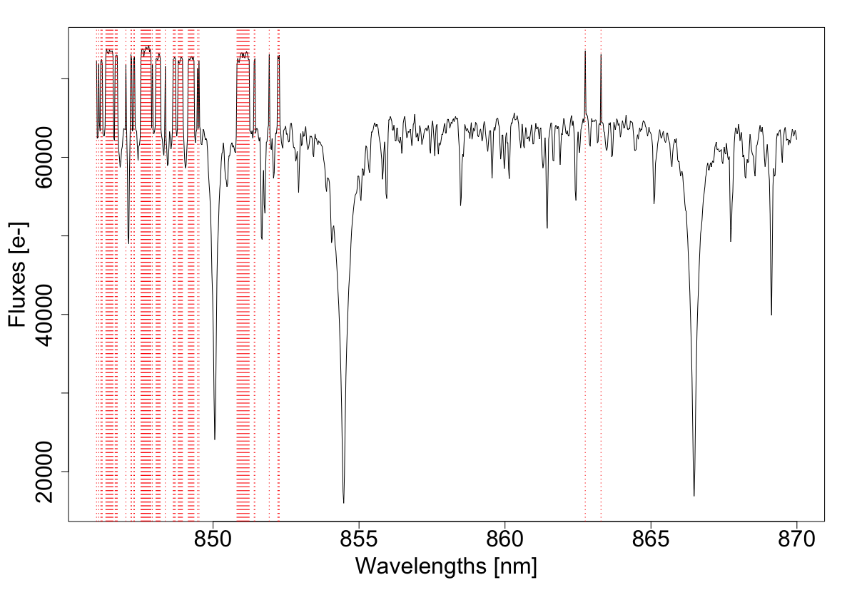
Figure 2: Saturation in an RVS spectrum. The CCD spectrum shown (in units of e^- per 4.4 sec exposure) was obtained from the summing in the AC direction of a 2D-window spectrum including saturated AC-central pixels. The resulting 1D spectrum, which presents 99 saturated samples (marked in red), was discarded by the pipeline. The visible jumps (of $\sim 8000\,\mathrm{e}^{-}$) originate from AC-central pixels exceeding 50 000 ADU (see Sect. 3.1). The corresponding star has ${\tt grvs\_mag}=3.471\pm 0.005$ mag, $T_{\rm eff}=4735$ K, $\log g=1.45$, and ${\rm[Fe/H]}=-0.13$.

3.2 Estimation of the stray-light background

The RVS spectra are contaminated by a diffuse background dominated by solar stray light caused by diffraction from detached fibres in the sunshield (Cropper et al. 2018). While stray-light contamination varies over time and also with position in the focal plane, it follows, for the most part, a relatively stable pattern related to the satellite rotation phase. Crowding effects also contribute to the background estimation: in crowded regions, such as during Galactic plane scans, the level of diffuse light contributing to the background is higher.

The accuracy and precision of the background measurement impact estimates of the total flux in the individual RVS spectra. The precision of the background estimation was improved in the DR3 pipeline through regular calibrations and the use of information outside the filter passband (i.e. at wavelengths below 843.2 nm and above 874.2 nm) in faint-star spectra to increase the number of individual background measurements.

Specifically, the background level was estimated every five spacecraft revolutions (i.e. every 30 hr). On each occurrence, the background was measured using the fluxes of so-called virtual objects (VOs; corresponding to empty windows with only background signal), together with flux measurements at the outer edges of the spectral windows of stars fainter than $G_{\mathrm{RVS}}^{\rm{onboard}}=15$ mag. The background associated with each RVS spectrum is the median flux computed using all clean VOs and faint stars in a large area around the star of interest, over a period of $\pm 6$ revolutions ($\pm 36$ hr) around the time of estimation. The area corresponds to 36 seconds of scan (per 6 hr revolution) including the star position, which samples 36 600 pixels in the AL direction (i.e. $\sim 2160^{\prime\prime}$) and 251 pixels in the AC direction ($\sim 45^{\prime\prime}$). We note that this procedure smoothes out any local variation of the background level over the considered area, as well as any temporal variation over a period of 72 hr (see section 5.2 of Sartoretti et al. 2018 for a detailed description of the background estimation algorithm).

The standard deviation of residuals around the median background estimate amounts to typically $3.15$ e^- sample^-1 in a 4.4 s exposure. This yields a typical uncertainty of $\pm$702 $\mathrm{e}^{-}\mathrm{s}^{-1}$ in the estimated background flux integrated over an RVS spectrum (about 980 samples). Hence, the background flux uncertainty for a single RVS-CCD spectrum is similar to the expected flux of a star with ${\tt grvs\_mag}=14.1$ mag (for which the flux uncertainty would therefore be of 100%).

3.3 Contamination from nearby sources

Some light from nearby sources may enter the RVS-spectrum window of the target source, leading to overestimation of the flux. Here, ‘nearby’ is meant in the focal-plane reference system: the two Gaia telescopes share the same focal plane (Gaia Collaboration et al., 2016), and nearby sources in the focal plane may come from the two different fields of view (FoVs) and be physically very far apart.

The relative distance between the contaminant and the target source in the focal plane is epoch-dependent. An RVS window may or may not have been assigned to the contaminant during a specific satellite scan. This is because of the onboard limit on the number of RVS spectra that can be obtained simultaneously, and occurs when one of the Gaia FoVs scans a crowded region of the sky. We define as ‘contamination area’ the area in the focal plane centred on the target source that extends over twice the size of the regular window. This contamination area corresponds to about 2592 AL $\times$ 21 AC pixels, or 152.93^′′ AL $\times$ 3.74^′′ AC. Nearby sources in the contamination area have a different impact on the target window depending on whether or not they have an RVS window. The two cases are therefore treated differently in the pipeline:

1. Contaminants with an RVS window generate truncations in the target source window (because the two windows partly overlap). This type of contamination is naturally accounted for by not using the target spectra with truncated windows. As an exception, 2D windows (pertaining to very bright stars with $G_{\mathrm{RVS}}^{\rm{onboard}}\leq 7$; see figure 1 of Sartoretti et al., 2018) are not truncated even if they are in conflict with other source windows. Contamination of 2D window spectra by relatively bright nearby sources is rare in practice and is ignored by the pipeline.

2. Contaminants without an RVS window do not generate any window conflict or window truncation. Potential contaminants are identified as transits of Gaia-catalogue sources brighter than $G_{\mathrm{RVS}}^{\rm{ext}}=15$ (fainter contaminants are ignored) and without an RVS window, based on the ‘ObjectLogsRVS’ files produced on board. The predicted AL and AC positions of the potential contaminants are computed by projecting the known astrometric coordinates of the source onto the focal plane, taking into account the satellite attitude and geometry. The effective contaminants are defined as the sources located in the contamination area around the target and which are sufficiently bright relative to the target, that is, brighter than $G_{\mathrm{RVS}}^{\rm{ext}}$ (target)+3. Transits of target sources with such contaminants are removed, while those of target sources with fainter contaminants are flagged ‘faint-contaminated’ and are used to estimate grvs_mag.

A total of about 135 million CCD spectra were removed because of contaminants without an RVS window.

With this procedure, for most of the target stars fainter than $G_{\mathrm{RVS}}^{\rm{onboard}}=7$, we expect to exclude all transits affected by contaminants closer than $\sim 1\,.87^{\prime\prime}$ and, depending on the satellite scan direction, at least part of the transits affected by contaminants at distances between $\sim 1.87^{\prime\prime}$ and $\sim 76.46^{\prime\prime}$.

Potential contamination from relatively bright sources (with or without an RVS window) located outside the contamination area is ignored in the pipeline. Neither the RVS filter response nor the LSF-AC was calibrated significantly outside the RVS window. Based on the on-ground data and extrapolation of the LSF-AC calibration, a contaminant just outside the contamination area is expected to contaminate the target window with less than $10^{-4}$ of its flux in the AL direction, and with less than $\sim 2$% of its flux in the AC direction (i.e. to have more than 0.2 mag of contamination on the target source, a contaminant located outside the contamination area must be at least 2.5 mag brighter than the target; very bright contaminant sources outside the contamination area can therefore still contaminate targets at the faint end). Also ignored by the pipeline are the potential contaminants with no RVS window and no $G_{\mathrm{RVS}}^{\rm{ext}}$ estimate (having changed source identifiers since DR2), and of course, those not present in the Gaia-source catalogue at all (not observed by Gaia).

Finally, a validation procedure based on the filters described in Sect. 6.2 eliminated many spurious estimates of grvs_mag affected by contamination from bright nearby sources, including outside the contamination area.

4 grvs_mag estimation from the RVS spectra

4.1 Zero-point calibration

The zero-point is calibrated every 30 hr in each of the 24 RVS ‘configurations’ (corresponding to 12 CCD in two FoVs), based on the reference magnitudes of a set of calibrator stars. The calibrator stars are the 103 865 stars in the Hipparcos catalogue (Perryman et al., 1997) with reference magnitudes brighter than $G_{\mathrm{RVS}}^{\rm{ref}}=10$ mag and expected to be constant from Gaia-DR2 photometric data. $G_{\mathrm{RVS}}^{\rm{ref}}$ is computed using the transformation provided in Jordi et al. (2010):

$$G_{\mathrm{RVS}}^{\mathrm{ref}}=V-0.0501-1.1667(V-I)+0.0052(V-I)^{2}+0.0011(V-I)^{3}\,,$$ (1)

where $V$ and $I$ are the magnitudes in the Hipparcos catalogue.

For a given ‘Calibration Unit’ (CaU; corresponding to 30 hr of observations in the same RVS configuration), the TotFlux of each calibrator star observed with the RVS is computed from the spectrum as described in Sect. 3.1. This allows the zero-point to be estimated as

$$ZP_{\rm{spec}}=G_{\mathrm{RVS}}^{\mathrm{ref}}+2.5\log({\it TotFlux})\,.$$ (2)

The global CaU zero-point is taken to be the median $ZP_{\rm{spec}}$ over all exploitable calibrator spectra (typically 150 to 200),

$$ZP_{\rm{CaU}}={\rm Med}(ZP_{\rm{spec}}),$$ (3)

and the global associated uncertainty the robust dispersion, $\sigma_{ZP_{\rm{CaU}}}=\frac{P(ZP_{\rm{spec}},84.15)-P(ZP_{\rm{spec}},15.85)}{2}$ , where $P(ZP_{\rm{spec}},84.15)$ and $P(ZP_{\rm{spec}},15.85)$ are the 84.15^th and the 15.85^th percentiles of the $ZP_{\rm{spec}}$ distribution.

Figure 3 shows the zero-points of all the CaUs obtained during the DR3 observing period in one of the Gaia CCDs. The time sequence of $ZP_{\rm{CaU}}$ values defines the temporal variation of the zero-point, noted $ZP(t)$, which can be modelled with second-degree polynomial trending functions, as illustrated. Generalising over all CaUs, the $ZP$ may be obtained from such functions for any RVS spectrum observed at any time and in any configuration. It is worth noting that, in the future DR4, estimates of the $ZP$ dispersion will be improved by informing the pipeline with products made available by DR3, such as reference synthetic magnitudes computed using externally calibrated low-resolution spectra from the red photometer (Montegriffo et al., 2022) convolved with the $G_{\rm RVS}$ passband derived in Sect. 7 below.

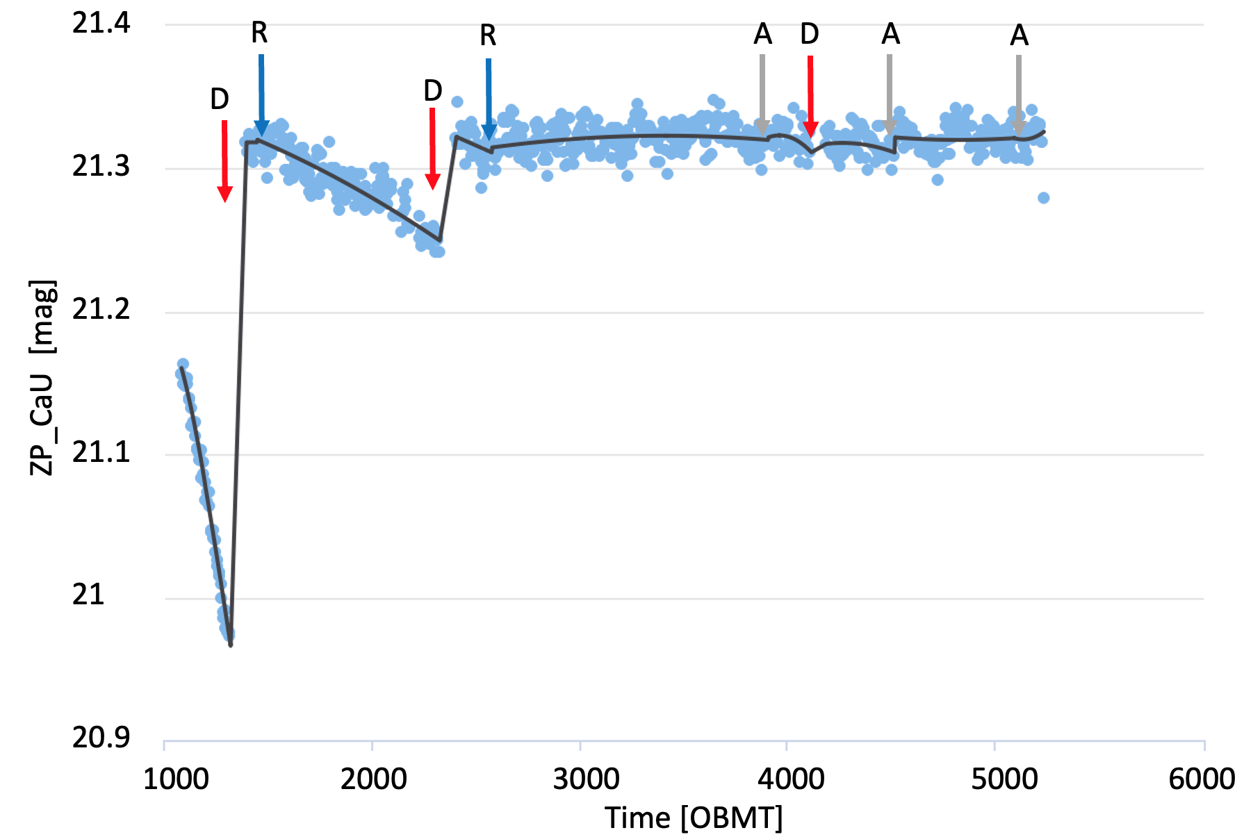
Figure 3: $G_{\rm RVS}$ zero-point plotted against OBMT. The blue points represent the $ZP_{\rm CaU}$ estimates (from Eq. 3) every 30 hr for the CCD in row 6, strip 2, and FoV 2 (see figure 1 of Sartoretti et al., 2018) over the DR3 observing period. The black line is the calibration model for $ZP(t)$. The arrows indicate break points between which the calibration model is fitted. The break points correspond to the following events: decontaminations (red arrows), refocus (blue arrows), and discontinuities in the astrometric solution (grey arrows). At the beginning of the mission, the Gaia optics suffered from heavy water ice contamination, which resulted in rapid degradation of the ZP. The first two decontamination events, at OBMT 1317 and 2330, produced a significant improvement in ZP. After the second decontamination event, the ZP stabilised, and the third decontamination event, which is also the last one performed on Gaia, resulted in no significant improvement. The other events have no significant effect on the ZP.

4.2 grvs_mag estimation

The grvs_mag magnitude of a star is computed on the basis of epoch magnitudes estimated each time the star is observed by the RVS. An epoch magnitude is defined as the median of the three magnitudes estimated from the three CCD spectra acquired when the star is scanned by the RVS (see figure 1 of Sartoretti et al., 2018), that is,

$$G^{\rm{epoch}}_{\mathrm{RVS}}={\rm Med}(G^{\rm{spec}}_{\mathrm{RVS}})\,,$$ (4)

where the individual magnitudes are estimated using the quantity TotFlux (Sect. 3.1) and the zero-point at time $t_{\rm obs}$ of observation (Sect. 4.1),

$$G^{\rm{spec}}_{\mathrm{RVS}}=-2.5\log({\it TotFlux})+ZP(t_{\rm obs})\,.$$ (5)

The source magnitude, grvs_mag, is defined as the median of all epoch magnitudes,

$${\tt grvs\_mag}={\rm Med}(G^{\rm{epoch}}_{\mathrm{RVS}})\,.$$ (6)

The formal error (assuming the normal law) on this median measurement is

$$\sigma_{\mathrm{Med}}=\sqrt{\frac{\pi}{2}}.\frac{\sigma(G^{\rm{epoch}}_{\mathrm{RVS}})}{\sqrt{\texttt{grvs\_mag\_ntransits}}}\,,$$ (7)

where $\sigma(G^{\rm{epoch}}_{\mathrm{RVS}})$ is the standard deviation of the epoch measurements and grvs_mag_ntransits is the total number of epochs. To estimate the uncertainty on grvs_mag, we add in quadrature to $\sigma_{\mathrm{Med}}$ an error of 0.004 mag to account for calibration-floor uncertainties:

$${\tt grvs\_mag\_error}=\sqrt{\sigma_{med}^{2}+0.004^{2}}\,.$$ (8)

We note that, as already mentioned in Sect. 3.1, our procedure to discard spectra with negative TotFlux and compute grvs_mag with the median of the epoch magnitudes leads to systematic underestimation of grvs_mag for faint stars. We attempt to quantify the resulting bias in Sect. 6.1 below. In the future DR4, we plan to avoid this bias by computing grvs_mag based on the median of the flux measurements (including negative ones).

5 $G_{\rm RVS}$ estimation from $G$ and $G_{\rm RP}$ 

As mentioned in Sect. 2.3, we had to resort to DR2 measurements of $G$ and $G_{\rm RP}$ (the magnitudes from Gaia astrometric images and red photometer), together with the transformation formulae in Eqs. (2) and (3) of Gaia Collaboration et al. (2018b), to estimate $G_{\mathrm{RVS}}^{\rm{ext}}$ required for pre-selecting RVS spectra for grvs_mag estimation. We can now use DR3 estimates of grvs_mag, $G$, and $G_{\rm RP}$ to update the formulae to estimate $G_{\rm RVS}$ from $G$ and $G_{\rm RP}$. We refer to this updated estimate of $G_{\mathrm{RVS}}^{\rm{ext}}$ as $G^{\rm{G,RP}}_{\mathrm{RVS}}$, which we compare with grvs_mag in Sect. 6.4 below.

It is important to note that the grvs_mag bandwidth defined over the 846–870 nm wavelength range (Fig. 1) is far narrower than the $G$, $G_{\rm BP}$, and $G_{\rm RP}$ bandwidths of standard Gaia photometry (see Fig. 7). Colour–colour relationships between grvs_mag, $G$, and $G_{\rm RP}$ were derived from a random sample of about 3 million sources well behaved in $G$, $G_{\rm BP}$, and $G_{\rm RP}$ excess flux (see Riello et al., 2021) and with ${\tt grvs\_mag\_error}<0.05$ mag.

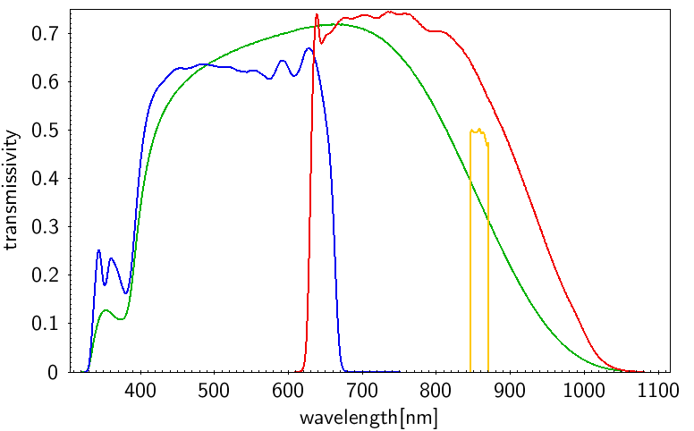
Figure 4: Passbands of the Gaia $G_{\rm BP}$ (blue curve), $G$ (green curve), and $G_{\rm RP}$ (red curve) filters (from Riello et al., 2021). The $G_{\rm RVS}$ passband (yellow curve), which defines grvs_mag, is that derived in Sect. 7.

The resulting cubic polynomial fits are:

for $-0.15\leq G-G_{\rm RP}\leq 1.2$,

$$G^{\rm{G,RP}}_{\mathrm{RVS}}-G_{\rm RP}=-0.0397-0.2852(G-G_{\rm RP})\\ -0.0330(G-G_{\rm RP})^{2}-0.0867(G-G_{\rm RP})^{3}\,,$$ (9)

and, for $1.2<G-G_{\rm RP}\leq 1.7$,

$$G^{\rm{G,RP}}_{\mathrm{RVS}}-G_{\rm RP}=-4.0618+10.0187(G-G_{\rm RP})\\ -9.0532(G-G_{\rm RP})^{2}+2.6089(G-G_{\rm RP})^{3}\,.$$ (10)

The root mean square errors in Eqs. (9) and (10) are 0.04 and 0.09 mag, respectively. The two polynomial relations are overplotted on the data in the colour–colour diagram of Fig. 5.

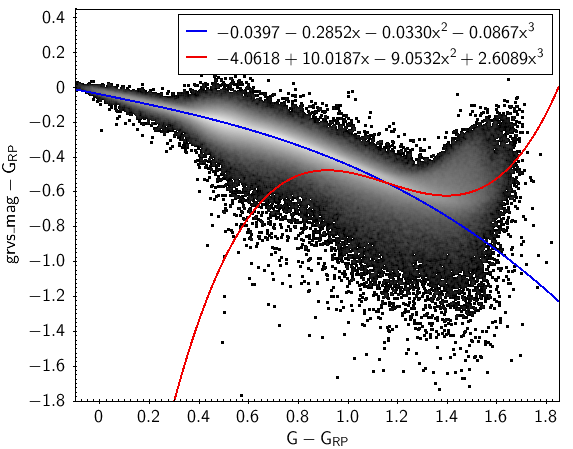
Figure 5: grvs_mag-$G_{\rm RP}$ versus $G-G_{\rm RP}$ colour–colour diagram for a random sample of about 3 million sources. Overplotted are the polynomial relations of eqs (9) and (10).

6 Validation of grvs_mag

6.1 Underestimate of grvs_mag at faint magnitudes

We now quantify how our removal of RVS spectra with negative total flux (${\it TotFlux}\leq 0$) in Sect. 4.2 impacts our measurements of grvs_mag. We achieve this by estimating grvs_mag for a set of simulated stars with known true magnitudes, noted $G^{true}_{\mathrm{RVS}}$, between 12 and 14.5 mag (in steps of 0.1 mag.). For each star, of true flux $10^{-0.4(G^{true}_{\mathrm{RVS}}-ZP)}$ (with $ZP=21.317$; see Sect. 7), we perform 39 realisations of the total RVS flux TotFlux assuming a normal distribution of the background subtraction uncertainty centred on 702 $\mathrm{e}^{-}\mathrm{s}^{-1}$. Here, 39 is the median number of individual RVS CCD spectra available to estimate grvs_mag for the sources in our sample (13 observation epochs $\times$ 3 CCDs). As in the procedure described in Sect. 4.2, we remove negative fluxes and compute a simulated grvs_mag, noted $G^{simu}_{\mathrm{RVS}}$, using Eq. (6). We produce 1000 such estimates of $G^{simu}_{\mathrm{RVS}}$ for each $G^{true}_{\mathrm{RVS}}$. In Fig. 6, we show the resulting median $G^{simu}_{\mathrm{RVS}}$ (along with its associated error) against $G^{true}_{\mathrm{RVS}}$. The median simulated grvs_mag starts to deviate from the true magnitude and become systematically brighter (by about 0.015 mag) at $G^{true}_{\mathrm{RVS}}=13.4$, reaching an offset of $\sim 0.14$ mag at $G^{true}_{\mathrm{RVS}}$=14.0. A similar magnitude term is reported in Babusiaux et al. (2022).

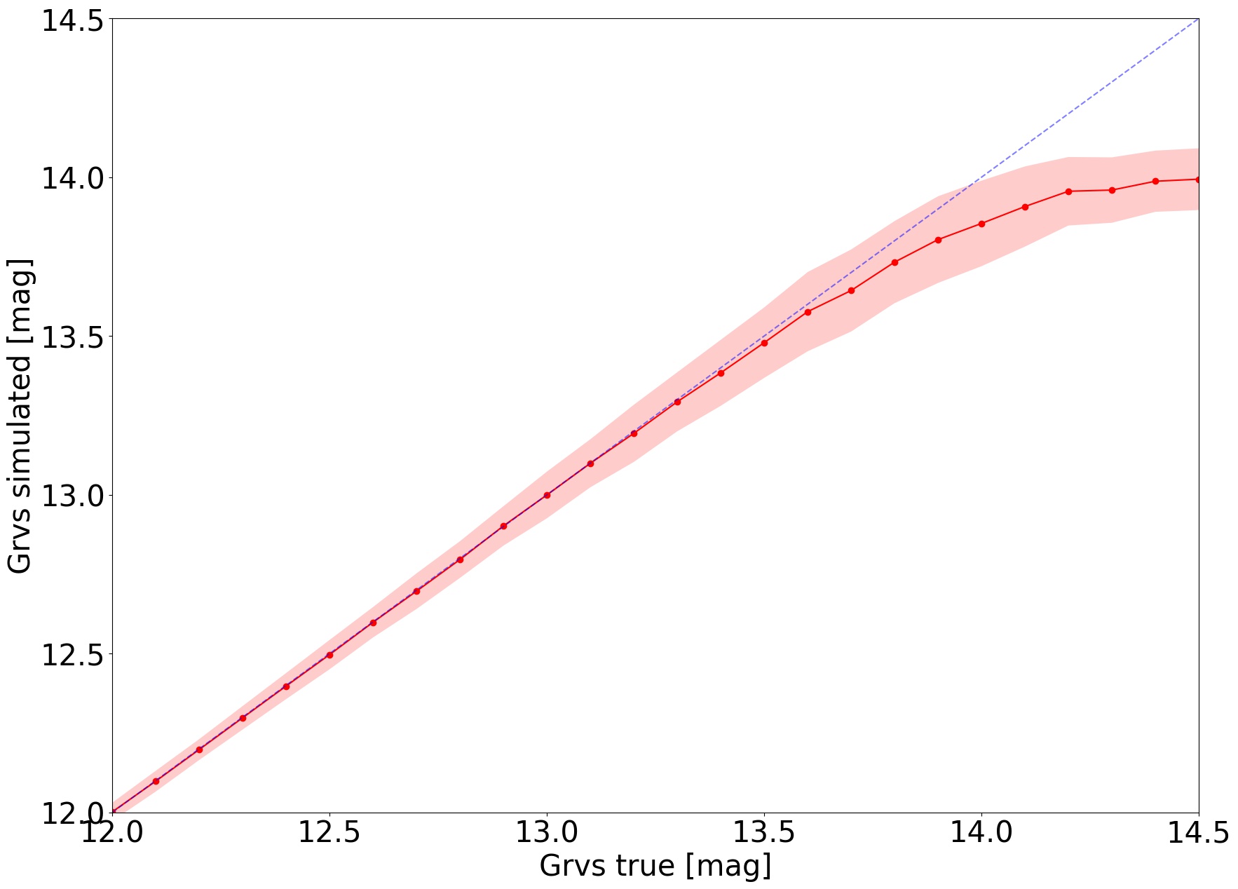
Figure 6: grvs_mag computed following the procedure outlined in Sect. 4.2, $G^{simu}_{\mathrm{RVS}}$, plotted against true magnitude, $G^{true}_{\mathrm{RVS}}$, for the simulations described in Sect. 6. The red line shows the median relation from 1000 realisations, and the shaded area the associated error. The dashed blue line shows the identity relation. The estimated magnitude becomes systematically brighter than the true one for $G^{true}_{\rm RVS}\mathrel{\hbox to0.0pt{\lower 3.5pt\hbox{$\mathchar 536\relax$}\hss}\raise 1.5pt\hbox{$\mathchar 318\relax$}}13.3$. The limiting magnitude of the stars processed for DR3 corresponds to $G^{true}_{\mathrm{\rm RVS}}=14$.

6.2 Validation filtering of grvs_mag

After completion of the DR3 processing of RVS data, a validation campaign was led to identify potentially erroneous data and filter these out from publication (in practice, the deemed erroneous data are nullified). Of the $\sim$37.1 million grvs_mag measurements produced by the pipeline, $\sim$4.9 million were nullified in this way, leading to the publication of about 32.2 million grvs_mag values in DR3. In the following paragraphs, we describe the filters applied to validate these measurements.

As mentioned in Sect. 1, the primary product of the RVS pipeline is the radial_velocity, and all filters applied to nullify spurious radial velocity measurements were applied to all pipeline products, including grvs_mag. The radial_velocity filter criteria are listed in the online documentation (Sartoretti et al., 2022, section 6.5.2.1) and described in detail in Katz et al. (2022) and Babusiaux et al. (2022). Most radial_velocity filters were beneficial also for grvs_mag, leading to the removal of many spurious grvs_mag measurements contaminated by nearby relatively bright sources located also outside the contamination area considered in the pipeline (Sect. 3.3). Also nullified were the grvs_mag measurements of potential SB2 stars (i.e. for which double lines are detected in at least 10% of epoch spectra), potential emission-line stars (i.e. with emission lines detected in more than 30% of epoch spectra), and stars with S/N $<2$ in the mean spectrum over all transits. On the other hand, radial_velocity filters also removed stars with potentially good-quality grvs_mag measurements, such as hot and cool stars, for which radial velocity measurements were deemed insufficiently accurate. These stars are selected based on their effective temperature ($T_{\rm eff}$) stored in the parameter rv_template_teff. Specifically, grvs_mag was nullified for faint hot stars with ${\tt grvs\_mag}>12$ mag and $T_{\rm eff}\geq 7000$ K; for bright hot stars with ${\tt grvs\_mag}\leq 12$ mag and $T_{\rm eff}>14,500$ K; and for cool stars with $T_{\rm eff}<3100$ K.

Additional filters were applied to identify and nullify other spurious estimates of grvs_mag. This includes about $9.4\times 10^{5}$ stars with too few $G^{\rm{epoch}}_{\mathrm{RVS}}$ measurements, that is, with ${\tt grvs\_mag\_nbtransits}<3$ for faint stars with ${\tt grvs\_mag}\geq 13$ mag, and ${\tt grvs\_mag\_nbtransits}\leavevmode\nobreak\ <2$ for brighter stars; about $1.5\times 10^{5}$ stars fainter than ${\tt grvs\_mag}=14.1$ mag, corresponding to the faintest magnitude measurable in a single CCD spectrum given the uncertainties in background-flux estimation (Sect. 3.2); and another $\sim 4.4\times 10^{4}$ stars for which a flagging error in the pipeline procedure described in Sect. 3.3 prevented identification of a bright contaminating source. This error —which led to a bright contaminant being ignored when a faint contaminant was also found— affected only bright targets with ${\tt grvs\_mag}<12$ mag. To account for this, and given that stars with ${\tt grvs\_mag}\leq 10.5$ mag rarely have bright contaminants, all stars fainter than 10.5 mag and with all their transits flagged ‘faint contaminant’ had their grvs_mag nullified.

Overall, about 3.8 million grvs_mag measurements were nullified by the radial velocity filters, and another 1.1 million by the above additional grvs_mag filters. The vast majority of these 4.9 million cases (93%) pertain to faint stars, with roughly 11.5% of all stars fainter than ${\tt grvs\_mag}=12$ removed, compared to $\sim 3.6$% of brighter stars. For reference, we show in Figs. 7 and 8 the distributions of effective temperature ($T_{\rm eff}$) and number of epoch measurements (grvs_mag_nbtransits) for the 32.2 million stars with grvs_mag measurements.

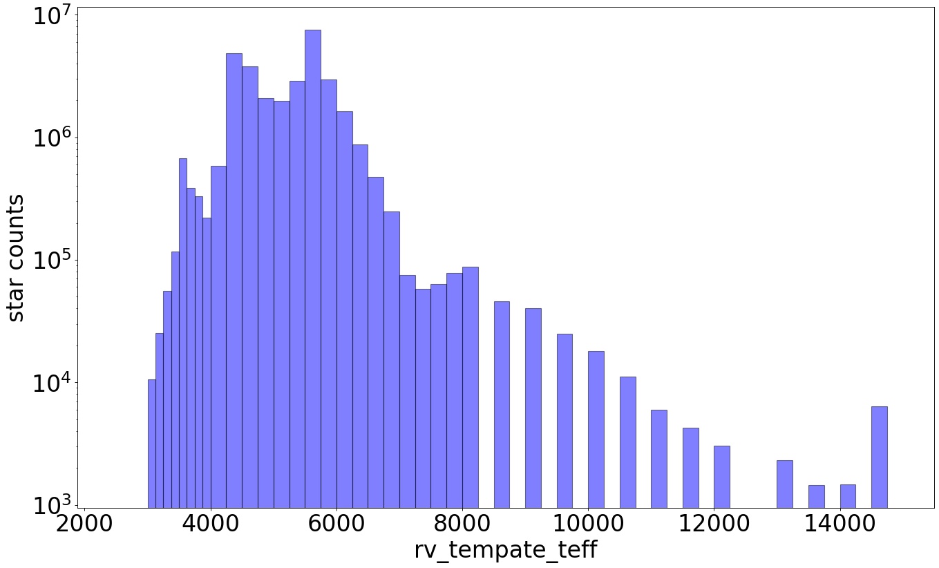
Figure 7: Distribution of effective temperature ($T_{\rm eff}$, estimated as described in footnote 9) for the 32.2 million stars with grvs_mag measurements published in DR3. The minimum $T_{\rm eff}$ is 3100 K, the maximum is 14 500 K, the median is 5250 K, and the mean is 5097 K.

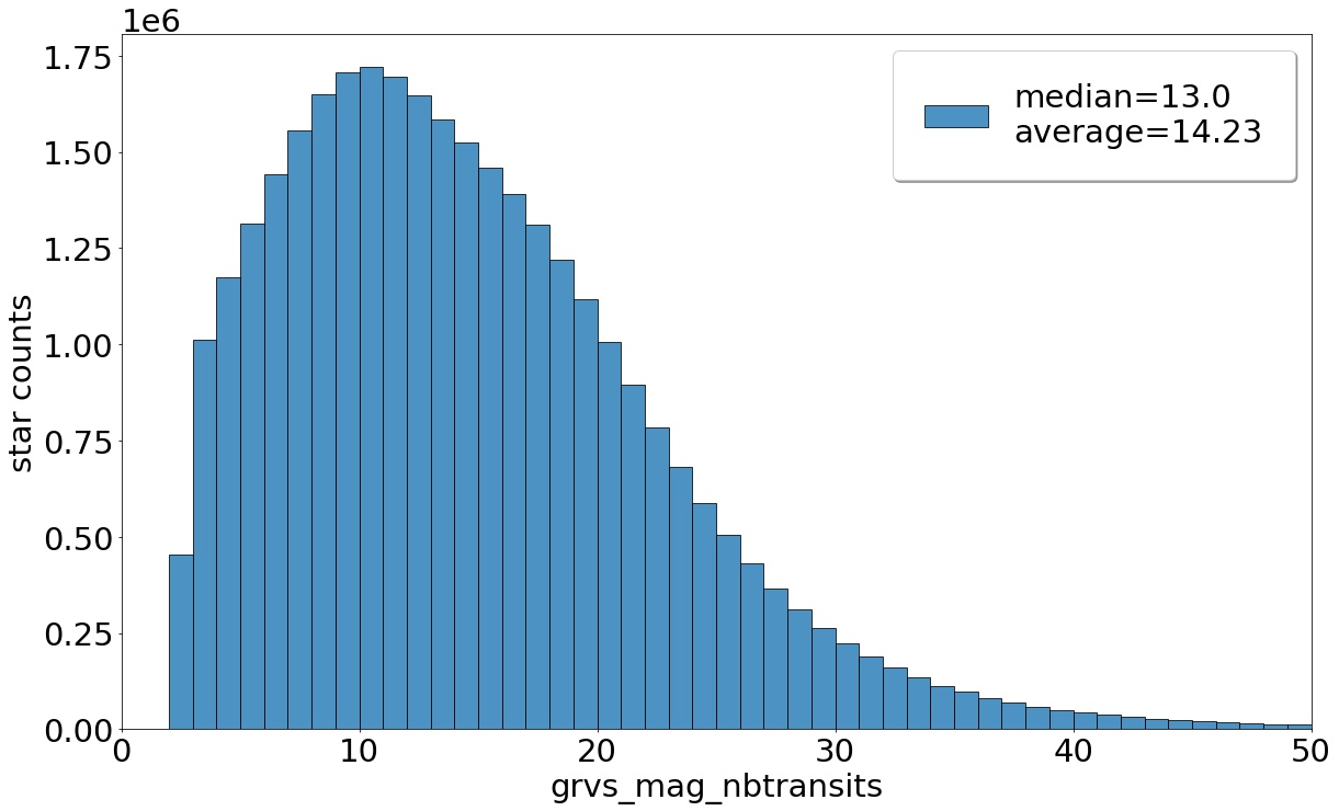
Figure 8: Distribution of the number of epoch observations (grvs_mag_nbtransit) for the 32.2 million stars with grvs_mag measurements published in DR3. The minimum grvs_mag_nbtransit is 2, the maximum is 219, the median is 13, and the mean is 14.23. About 58 000 sources have ${\tt grvs\_mag\_nbtransit}>50$.

Figure 9 (bottom panel) shows the sky distribution of grvs_mag_nbtransit, the median number of epoch measurements per source being 13.

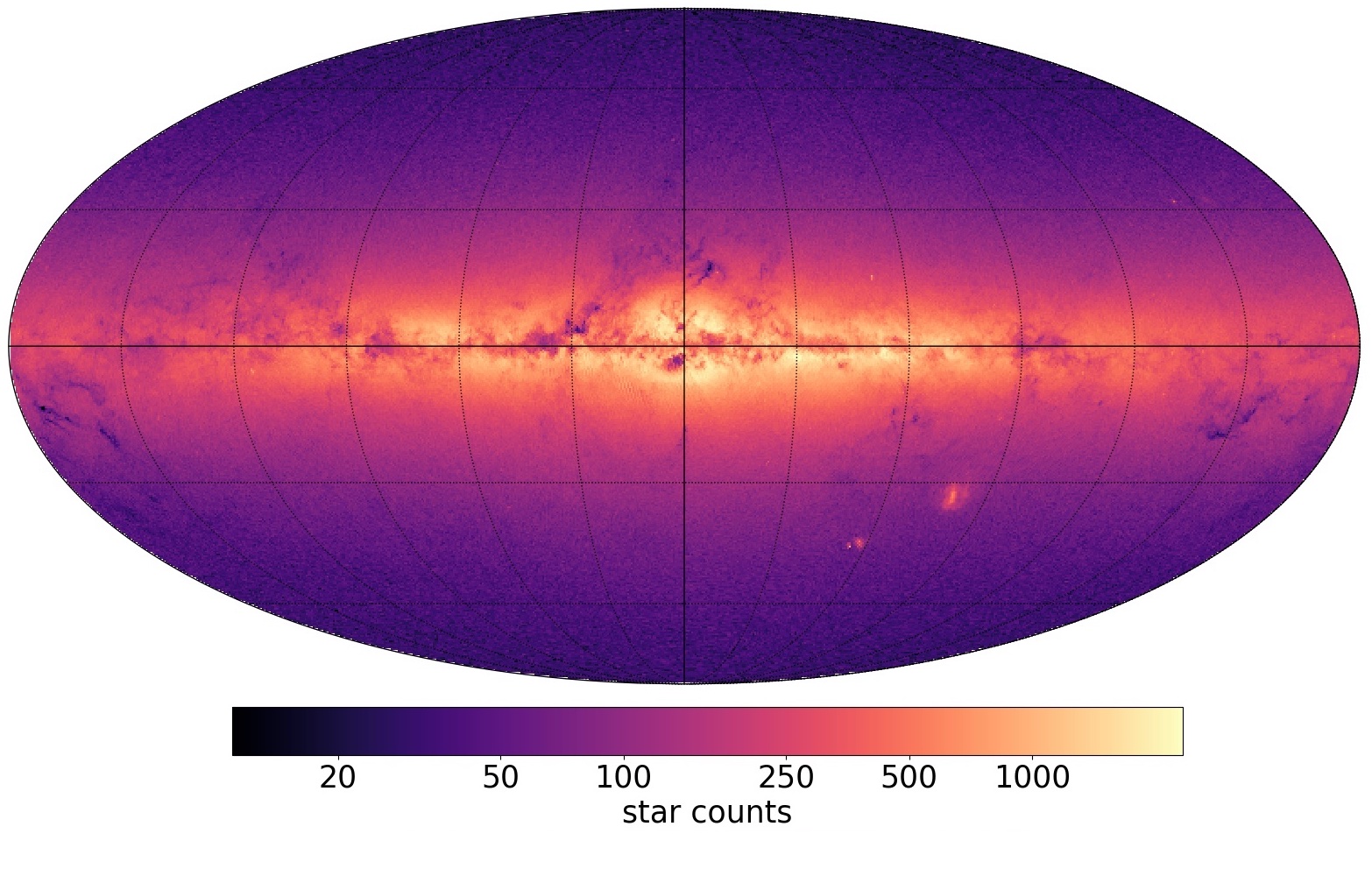
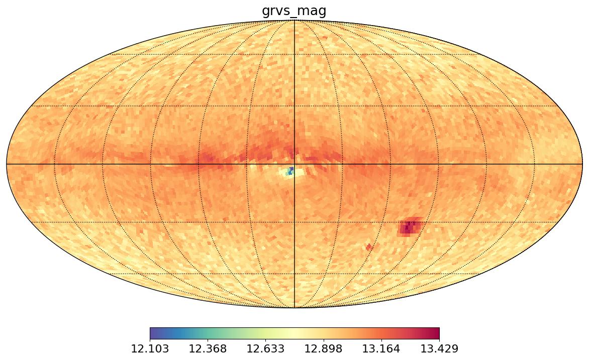
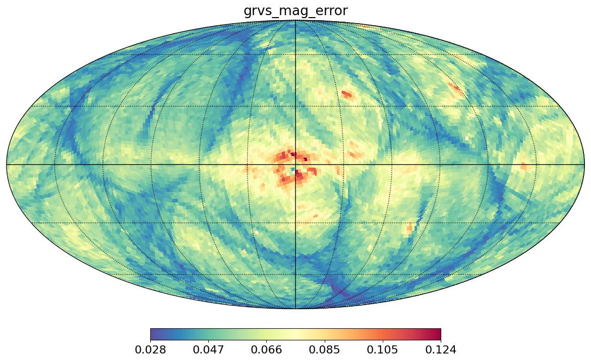
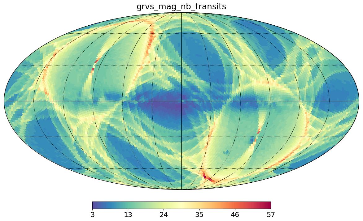
Figure 9: HEALPix maps in Galactic coordinates for the 32.2 million stars with grvs_mag measurements published in DR3. From top to bottom: Source density over 0.2 square degrees (i.e. HEALPix level 7); median grvs_mag over 3.36 square degrees (HEALPix level 5); median grvs_mag_error over 3.36 square degrees (HEALPix level 5); and median grvs_mag_nb_transits over 3.36 square degrees (HEALPix level5).

While we expect most spurious grvs_mag measurements to have been cleaned through pipeline processing and the above validation procedure, some published measurements of faint stars with few observations, that is, with ${\tt grvs\_mag\_nbtransits}\mathrel{\hbox to0.0pt{\lower 3.5pt\hbox{$\mathchar 536\relax$}\hss}\raise 1.5pt\hbox{$\mathchar 316\relax$}}5$, could still be potentially spurious. A small grvs_mag_nbtransits is typical for stars in crowded sky regions (Sect. 6.3), and the few remaining observations may be affected by contamination that has gone unnoticed (the fainter the star, the fainter and more numerous the potential contaminants, such as sufficiently bright stars outside the contamination area; see Sect. 3.3). Faint stars are also significantly affected by background estimation errors, which are not averaged out when epoch observations are few.

6.3 Completeness of grvs_mag

The maps of Fig. 9 provide an illustration of the completeness of grvs_mag measurements across the sky. The sky distribution of the 32.2 million sources with DR3 grvs_mag measurements (top panel) shows that, unsurprisingly, the densest sampling is achieved in the Galactic plane and the two Magellanic clouds. The darker areas on this map correspond to regions obscured by dust lanes and to regions with extremely high stellar density, where clean grvs_mag measurements are particularly limited by strong contamination (Sect.3.3), in addition to the constraint on the maximum number of spectra that can be obtained simultaneously (Sect. 2.1). The brightest areas on this map correspond to regions with high density of stars with grvs_mag measurements, but in such regions, the number of epoch measurements (grvs_mag_nbtransits) is also lower, as revealed by the dark areas in the bottom map of Fig. 9 (the bright structures on this map show the imprints of the Gaia scanning law). This is again because of the increased contamination and the limit to the number of RVS spectra that can be acquired in crowded areas. In such cases, priority is given to bright sources (Sect. 2.1). For this reason, only the very few, brightest stars are observed close to the Galactic centre, and the median magnitude of this region, shown in the second map of Fig. 9, is brighter than the average.

We can estimate the completeness of grvs_mag measurements as the ratio of the number of stars with such measurements to that of stars with standard $G$ measurements. We compute this ratio in bins of 0.1 $G$ magnitude and present the results in Fig. 10. The completeness is better than 80% over the full range of $G$ magnitudes from roughly 6 to 14 mag. Different features in the curve can be traced back to the procedure used to compute grvs_mag. The low completeness at the bright end ($G<4$ mag) results from the removal of all saturated RVS spectra of bright stars (i.e. spectra presenting more than 40 saturated pixels). The relative drop in completeness at $G\mathrel{\hbox to0.0pt{\lower 3.5pt\hbox{$\mathchar 536\relax$}\hss}\raise 1.5pt\hbox{$\mathchar 318\relax$}}8.5$ mag ($G_{\mathrm{RVS}}^{\rm{onboard}}\mathrel{\hbox to0.0pt{\lower 3.5pt\hbox{$\mathchar 536\relax$}\hss}\raise 1.5pt\hbox{$\mathchar 318\relax$}}7$ mag) corresponds to the transition from 2D to 1D acquisition windows (see figure 1 of Sartoretti et al., 2018). The 2D windows are never truncated or excluded (when not saturated), while 1D windows may be truncated and then excluded. A star around this transition may, at some epoch, have $G_{\mathrm{RVS}}^{\rm{onboard}}$ slightly brighter than 7 mag and get a 2D window, and at some other epochs may have a slightly fainter magnitude and get a 1D window. In the latter case, a spike of the source PSF may occasionally cause the onboard software to assign an overlapping window to that spike (interpreted as a nearby source) and truncate the source window. The occurrence of such spurious detections drops sharply for faint stars (see Sartoretti et al., 2018, section 3.2), as shown by the rise in completeness at $G\mathrel{\hbox to0.0pt{\lower 3.5pt\hbox{$\mathchar 536\relax$}\hss}\raise 1.5pt\hbox{$\mathchar 318\relax$}}9$ in Fig. 10. The drop in completeness at $G\mathrel{\hbox to0.0pt{\lower 3.5pt\hbox{$\mathchar 536\relax$}\hss}\raise 1.5pt\hbox{$\mathchar 318\relax$}}12.5$ (corresponding in median to ${\tt grvs\_mag}\sim 12$) reflects the more effective filters applied to faint stars relative to bright stars (see Sect. 6.2).

We note that, because of the additional filters applied to grvs_mag measurements relative to radial_velocity measurements (Sect. 2.4 and Sect. 6.2), about 1.6 million sources with radial_velocity measurements do not have grvs_mag measurements.

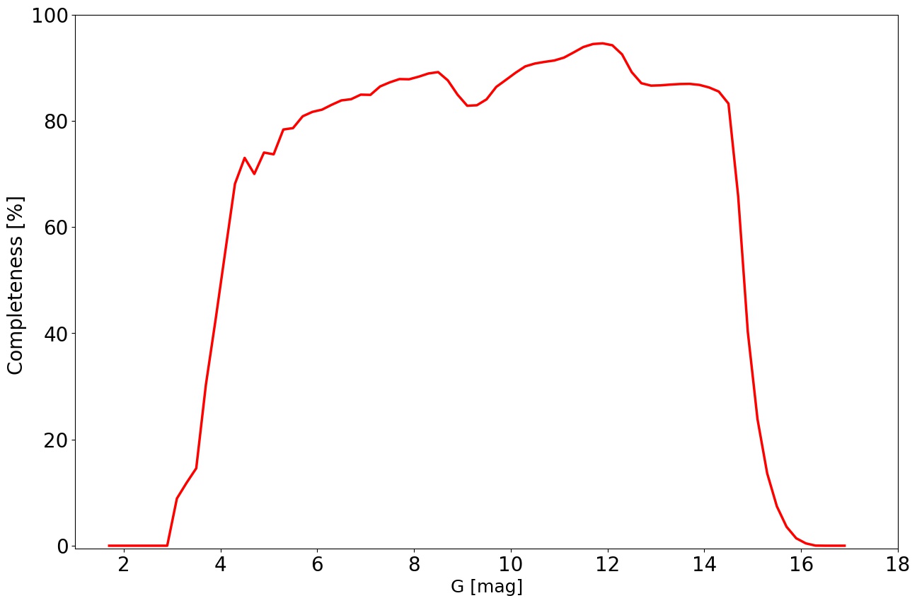
Figure 10: Ratio of the number of stars with grvs_mag measurements to that of stars with standard $G$ measurements, in bins of 0.1 $G$ magnitude.

6.4 Accuracy and precision

We can estimate the accuracy (systematic uncertainty) of grvs_mag in first approximation by comparison with $G^{\rm{G,RP}}_{\mathrm{RVS}}$ (Sect. 5). Figure 11 shows the ${\tt grvs\_mag}-G^{\rm{G,RP}}_{\mathrm{RVS}}$ residuals as a function of grvs_mag. These residuals are sensitive to uncertainties in both grvs_mag and $G^{\rm{G,RP}}_{\mathrm{RVS}}$. The median residuals in bins of $\Delta({\tt grvs\_mag})=0.1$ mag in the blue range of $G-G_{\rm RP}$ colours (Eq. 9; solid line in Fig. 11) exhibit a small trend with grvs_mag, while the trend is more pronounced for the median residuals in the red range of colours (Eq. 10; dashed line). For both ranges of colours, the apparent sudden rise in median residuals at ${\tt grvs\_mag}\mathrel{\hbox to0.0pt{\lower 3.5pt\hbox{$\mathchar 536\relax$}\hss}\raise 1.5pt\hbox{$\mathchar 318\relax$}}13.75$ mag is artificial and caused by the selection criterion $G_{\mathrm{RVS}}^{\rm{ext}}\leq 14$ mag (Sect.2.3).

The large majority ($\sim$ 93%) of the 32.2 million stars with grvs_mag measurements have blue $G-G_{\rm RP}$ colours, that is, $-0.15\leq G-G_{\rm RP}\leq 1.2$ mag (Sect. 5). The small trend in median ${\tt grvs\_mag}-G^{\rm{G,RP}}_{\mathrm{RVS}}$ residuals in Fig. 11 is reminiscent of the trend observed in $G-G_{\rm RP}$ versus $G$ (see Fig. 32 of Fabricius et al., 2021). A comparison with Hipparcos magnitude (Perryman et al., 1997) and Tycho2 colours (Høg et al., 2000) reveals no saturation issue for grvs_mag. The saturation corrections for $G$ and $G_{\rm RP}$ outlined in Appendix C.1 of Riello et al. 2021 do not reduce the trend. This is why the higher residuals at the bright end (where grvs_mag is slightly fainter than $G^{\rm{G,RP}}_{\mathrm{RVS}}$) seem mostly imputable to systematic errors in $G^{\rm{G,RP}}_{\mathrm{RVS}}$. Instead, the drop in residuals for faint stars with $12.2\mathrel{\hbox to0.0pt{\lower 3.5pt\hbox{$\mathchar 536\relax$}\hss}\raise 1.5pt\hbox{$\mathchar 316\relax$}}{\tt grvs\_mag}\mathrel{\hbox to0.0pt{\lower 3.5pt\hbox{$\mathchar 536\relax$}\hss}\raise 1.5pt\hbox{$\mathchar 316\relax$}}13.8$ mag (where grvs_mag is brighter than $G^{\rm{G,RP}}_{\mathrm{RVS}}$) is mostly caused by systematic errors in grvs_mag introduced by the rejection of spectra with ${\it TotFlux}<0$ (see also Sect. 6.1).

The remaining 7% ($\sim$ 2.2 million) of stars with grvs_mag measurements have red $G-G_{\rm RP}$ colours, that is, $1.2<G-G_{\rm RP}\leq 1.7$ (Sect. 5). As seen in Fig. 5 above, the relation (Eq. 10) to estimate $G^{\rm{G,RP}}_{\mathrm{RVS}}$ from $G$ and $G_{\rm RP}$ in the red range of $G-G_{\rm RP}$ colours is not as well constrained as that (Eq. 9) in the blue colour range, implying lower quality estimates of $G^{\rm{G,RP}}_{\mathrm{RVS}}$ in the red range. Indeed, stars with red $G-G_{\rm RP}$ colours tend to present few epoch observations (median ${\tt grvs\_mag\_nbtransits}=7$), characteristic of stars in dense regions (Sect. 6.3). These stars are mostly distributed in the Galactic disk, where both stronger dust obscuration (the $G$ and $G_{\rm RP}$ filters extending over bluer wavelengths than the grvs_mag passband) and uncaught contamination (Sect. 6.2) may contribute to making grvs_mag brighter than $G^{\rm{G,RP}}_{\mathrm{RVS}}$. This is the reason for the pronounced trend in median ${\tt grvs\_mag}-G^{\rm{G,RP}}_{\mathrm{RVS}}$ residuals for faint stars around $12.2\mathrel{\hbox to0.0pt{\lower 3.5pt\hbox{$\mathchar 536\relax$}\hss}\raise 1.5pt\hbox{$\mathchar 316\relax$}}{\tt grvs\_mag}\mathrel{\hbox to0.0pt{\lower 3.5pt\hbox{$\mathchar 536\relax$}\hss}\raise 1.5pt\hbox{$\mathchar 316\relax$}}13.8$ mag in Fig. 11 (dashed line). Instead, at the bright end, the median residuals indicate that grvs_mag is systematically fainter than $G^{\rm{G,RP}}_{\mathrm{RVS}}$, which reflects the prominence of cool stars ($T_{\rm eff}\mathrel{\hbox to0.0pt{\lower 3.5pt\hbox{$\mathchar 536\relax$}\hss}\raise 1.5pt\hbox{$\mathchar 316\relax$}}3500$ K) with positive gradients arising from the presence of TiO absorption in their spectra. This is further illustrated by Fig. 12, which shows the enhanced residuals affecting bright stars with $T_{\rm eff}\leq 3500$ K.

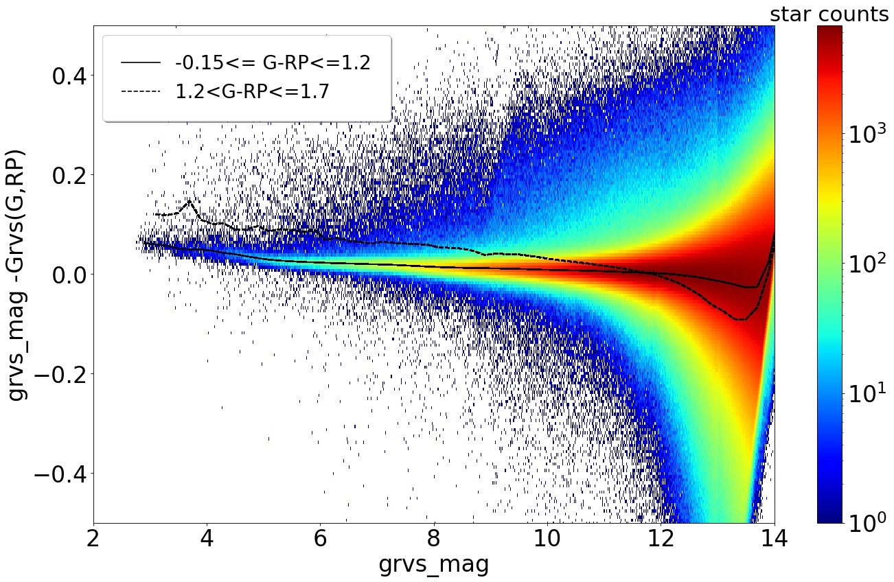
Figure 11: ${\tt grvs\_mag}-G^{\rm{G,RP}}_{\mathrm{RVS}}$ residuals plotted against grvs_mag. The black solid line shows the median residuals in bins of $\Delta({\tt grvs\_mag})=0.1$ mag for stars with blue $G-G_{\rm RP}$ colours ($-0.15\leq G-G_{\rm RP}\leq 1.2$ mag; Eq. 9), and the black dashed line the median residuals for stars with red $G-G_{\rm RP}$ colours ($1.2<G-G_{\rm RP}\leq 1.7$; Eq. 10). The $G_{\mathrm{RVS}}^{\rm{ext}}\leq 14$ mag selection criterion to measure grvs_mag (Sect. 2.3) translates into a cut at ${\tt grvs\_mag}-G^{\rm{G,RP}}_{\mathrm{RVS}}={\tt grvs\_mag}-14$ in this diagram, resulting in the apparent rise of the median residuals at the faint end.

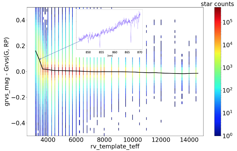
Figure 12: ${\tt grvs\_mag}-G^{\rm{G,RP}}_{\mathrm{RVS}}$ residuals plotted against effective temperature $T_{\rm eff}$ (rv_template_teff; see footnote 9) for stars with ${\tt grvs\_mag}\leq 12$ mag. The black line shows the median relation. For stars cooler than $T_{\rm eff}\sim 3500$ K, grvs_mag is fainter than $G^{\rm{G,RP}}_{\mathrm{RVS}}$. This is because of the positive gradient produced by TiO absorption in the spectra of such stars, as shown by the inset spectrum of a star with ${\tt grvs\_mag}=10.3$ and $T_{\rm eff}=3300$ K.

In Fig. 13, we show the internal precision grvs_mag_error as a function of grvs_mag for the 32.2 million stars with grvs_mag measurements. The distribution of grvs_mag_error on the sky is shown in the third panel of Fig. 9. A comparison with the distribution of the number of transits, grvs_mag_nbtransits (bottom panel of Fig. 9) indicates that, as expected, grvs_mag_error tends to be larger when grvs_mag_nbtransits is lower.

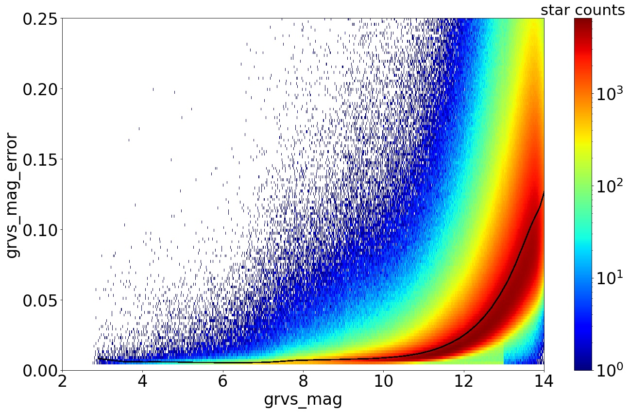
Figure 13: Internal precision: grvs_mag_error plotted against grvs_mag. The black line shows the median grvs_mag_error in bins of $\Delta({\tt grvs\_mag})=0.1$ mag. This indicates a median ${\tt grvs\_mag\_error}$ around 0.006 mag over the range $4\mathrel{\hbox to0.0pt{\lower 3.5pt\hbox{$\mathchar 536\relax$}\hss}\raise 1.5pt\hbox{$\mathchar 316\relax$}}{\tt grvs\_mag}\mathrel{\hbox to0.0pt{\lower 3.5pt\hbox{$\mathchar 536\relax$}\hss}\raise 1.5pt\hbox{$\mathchar 316\relax$}}6.5$ mag, increasing to $\sim$ 0.025 at ${\tt grvs\_mag}\sim 12$ mag, and $\sim$ 0.125 at ${\tt grvs\_mag}\sim 14$ mag.

7 Estimation of the $G_{\rm RVS}$ passband

We can estimate the passband of the effective $G_{\rm RVS}$ filter to which grvs_mag corresponds by comparing high-quality RVS spectra acquired for stars with existing reference spectra. We consider 21 stars from the Hubble Space Telescope archive of calibrated spectrophotometric standards (CALSPEC) (Bohlin et al., 2014, 2021 March Update) and 87 stars from the Next Generation Spectral Library (NGSL) spectrophotometric library (Heap & Lindler, 2016) which all have high-quality RVS data, that is, with ${\tt grvsmag\_error}<0.02$ mag and clean mean spectra in the 846–870 nm wavelength range (Fig. 1). To account for temporal variations of the zero-point (Sect. 4.1), we scale each RVS epoch spectrum according to the zero-point estimated at the time of observation, corresponding to a factor $10^{-0.4\leavevmode\nobreak\ ZP(t_{obs})}$. We ignore the lower quality epoch spectra obtained before the first decontamination (i.e. 1317 OBMT, Fig. 3). For each source, we then compute the spectrum averaged over all epochs, which we scale back to units of $\mathrm{e}^{-}\mathrm{s}^{-1}$using the median zero-point ($ZP=21.317$). In the resulting spectrum, denoted $F_{\mathrm{rvs}}(\lambda)$, the total flux in the 846–870 nm wavelength range is therefore $10^{-0.4({\tt grvs\_mag}-ZP)}$.

We seek the total RVS transmission $S(\lambda)$ such that

$$F_{\mathrm{rvs}}(\lambda)=PF_{\mathrm{ext}}(\lambda)S(\lambda)\,,$$ (11)

where $P$ is the telescope pupil area (0.7278 m²) and $F_{\mathrm{ext}}(\lambda)$ the reference flux-calibrated spectrum of the source (from CALSPEC or NGSL; converted to units of photons s^-1 m^-2).

To compare the RVS spectrum with the reference one, the RVS spectrum must be convolved to the (always lower) spectral resolution of the reference spectrum, and the reference spectrum must be shifted to the RVS radial velocity reference frame. To do so, the optimal Gaussian kernel width and radial velocity shift are selected through a minimum $\chi^{2}$ search in the 848–870 nm wavelength range, corresponding to the quasi-flat range of the RVS transmission. The Gaussian kernel found in this way incorporates the blurring caused by temporal variations of the radial velocity. Then, the RVS transmission can be estimated by simply dividing the RVS spectrum by the reference spectrum. In practice, to avoid unwanted border effects, the RVS spectrum must be divided by a first-guess transmission (taken to be the nominal pre-launch one) before convolution to the reference-spectrum resolution, and then re-multiplied by the same transmission. The process is iterative, the spectra of all sources being processed at each iteration (convergence is obtained after three iterations). After the first iteration, the transmission over the full RVS wavelength range is estimated as the median transmission over all sources. The $G_{\rm RVS}$ filter passband pertains to the 846–870 nm wavelength range used to compute $G_{\rm RVS}$. It is estimated through a B-spline median regression (cobs R package, Ng & Maechler, 2007), applying weights derived from the propagated errors of both the RVS and reference spectra. We note that five spectra found to be 5$\sigma$ outliers in their total flux were discarded.

The full transmission $S(\lambda)$ is presented in Fig. 14, together with the nominal pre-launch transmission. This shows that the observed transmission is better than the pre-launch estimate (by a factor of about 1.23) and slightly shifted to the blue. The $G_{\rm RVS}$ filter passband, which corresponds to this transmission in the 846–870 nm wavelength range, is available from the cosmos pages in footnote 8.

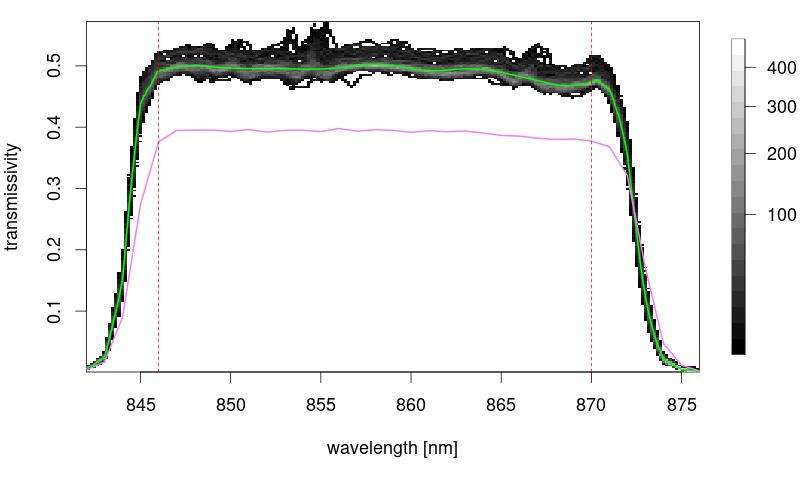
Figure 14: Global RVS transmission function $S(\lambda)$ (green line) corresponding to the median of 108 estimates derived from reference spectra (shown in the background with a grey scale indicating curve density). The purple curve shows the nominal pre-launch transmission, and the two red vertical lines the limits of the $G_{\rm RVS}$ passband.

By construction, the median zero-point to use with this filter is $ZP=21.317\pm 0.002$ mag (see above). This is consistent with the zero-point derived from the magnitude $m_{0}$ of the Vega spectrum $f_{\lambda}^{Vg}(\lambda)$ adopted for the $G_{\rm BP}$ and $G_{\rm RP}$ zero-point determination, converted to units of photons s^-1 nm^-1 m^-2,

$$m_{0}=2.5\log{\int Pf_{\lambda}^{Vg}(\lambda)S(\lambda)d\lambda}\,,$$ (12)

which leads to $m_{0}=21.321\pm 0.016$.

8 Examples of useful applications of grvs_mag

By design, the present study, which is dedicated to the description of grvs_mag published in DR3, belongs to the series of ‘Gaia-processing papers’, which reserve the scientific exploitation of DR3 data to the user community. In this section, we briefly illustrate some of the performances of grvs_mag measurements, which may be of interest for potential scientific applications.

8.1 Extinction

The sky distribution of the $G-{\tt grvs\_mag}$ colours of the 32.2 million stars with DR3 grvs_mag measurements, shown in Fig. 15, is sensitive to the distribution of extinction by interstellar dust.

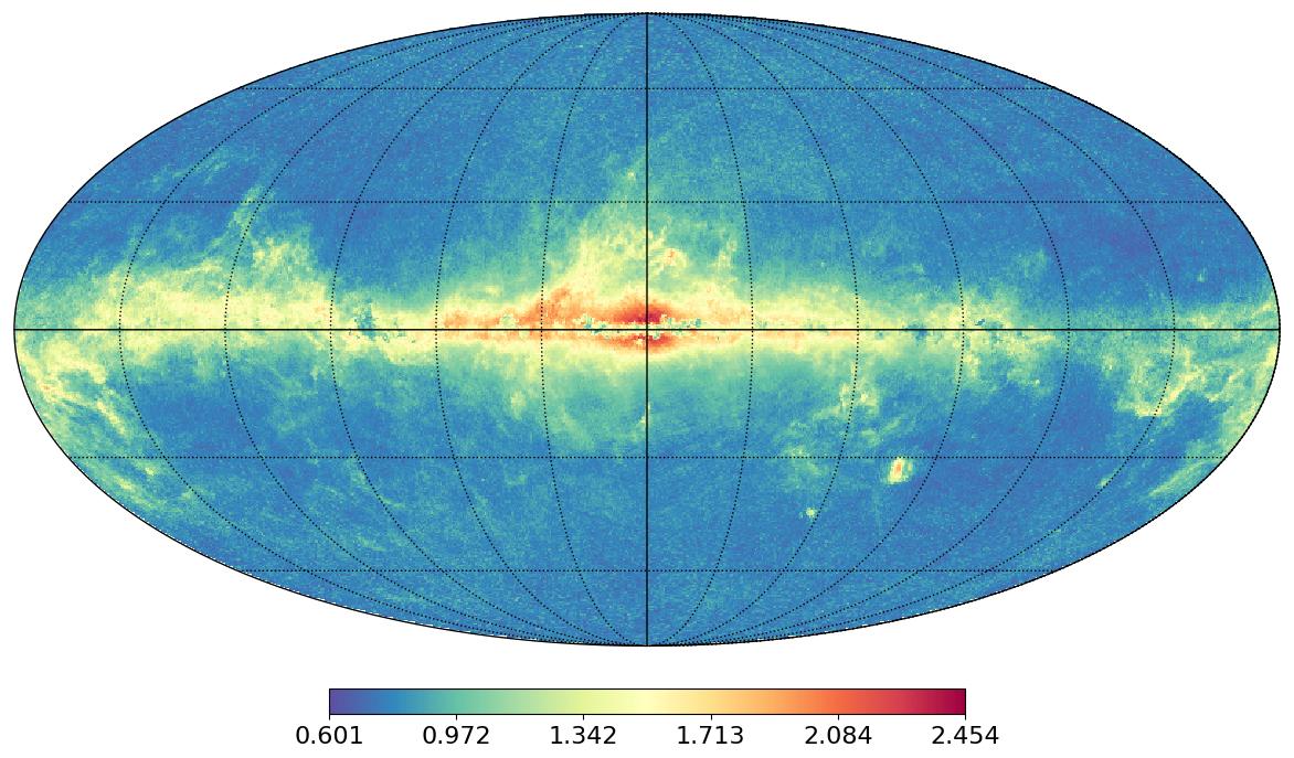
Figure 15: Median $G\ -{\tt grvs\_mag}$ colour in HEALPix map of level 7, highlighting the effect of extinction by interstellar dust.

The narrowness of the $G_{\rm RVS}$ filter (Fig. 7) makes the extinction coefficient in this band mostly independent of the spectral type of the star and the extinction itself, unlike for the $G_{\rm BP}$, $G$, and $G_{\rm RP}$ filters (see e.g. Jordi et al., 2010). Hence, grvs_mag is potentially useful for improving determinations of stellar atmospheric parameters. In fact, the derivation of these parameters from low-resolution, blue-, and red-photometer spectra suffers from a temperature–extinction degeneracy (Andrae et al., 2022), which can be broken with help from an extra constraint in the red.

Figure 16 shows the $G-{\tt grvs\_mag}$ versus $G_{\rm BP}-G_{\rm RP}$ colour–colour relation of stars of red clump stars with similar metallicity ($|\mathrm{[M/H]}+0.15|<2\sigma_{\rm[M/H]}$) from the APOGEE DR16 Red Clump catalogue (Bovy et al., 2014). This relation is primarily driven by extinction (we adopt here $G_{\mathrm{BP}}-G_{\mathrm{RP}}=1.2$ and $G-{\tt grvs\_mag}=0.95$ as the intrinsic Red Clump colours). Using the Fitzpatrick et al. (2019) extinction law, we find that the extinction coefficient in the RVS band at the central wavelength of the $G_{\rm RVS}$ filter is $k_{\mathrm{RVS}}=0.5385$. The extinction coefficients computed with the same extinction law for the $G$, $G_{\rm BP}$, and $G_{\rm RP}$ passbands are available from the cosmos pages. As the passbands for these filters are much larger than the $G_{\rm RVS}$ one (Fig. 7), their extinction coefficients depend sensitively on star colour and extinction itself, unlike $k_{\mathrm{RVS}}$ (which deviates by less than 0.2% up to $A_{0}=20$). The green line in Fig. 16 shows the resulting expected extinction effect on the $G-{\tt grvs\_mag}$ versus $G_{\rm BP}-G_{\rm RP}$ colours.

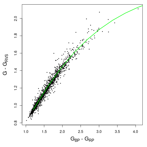
Figure 16: $G-{\tt grvs\_mag}$ versus $G_{\rm BP}-G_{\rm RP}$ colour–colour diagram of APOGEE DR16 Red Clump stars with similar metallicity. The green line shows the expected red clump star colour–colour relation driven by extinction, as computed using the Fitzpatrick et al. (2019) extinction law.

8.2 Stellar metallicity

As noted in Fig. 1, the $G_{\rm RVS}$ narrow-band filter is centred on the infrared CaII triplet, which, in ground-based observations, is contaminated by atmospheric H₂O-line absorption. grvs_mag provides useful information complementary to that obtained from the Gaia blue- and red-prism spectra, which can help to constrain stellar atmospheric parameters. We note that Bonifacio et al. (2018) predicted the potential of grvs_mag to constrain stellar metallicity. Figures 17 and 18 confirm the potential of the $G_{\rm RP}\ -{\tt grvs\_mag}$ colour as a metallicity diagnostic.

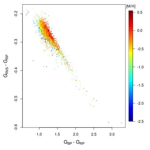
Figure 17: ${\tt grvs\_mag}-G_{\rm RP}$ versus $G_{\rm BP}\ -G_{\rm RP}$ colour–colour diagram for the APOGEE DR16 (Ahumada et al., 2020) giants with low extinction ($A_{0}<0.05$, according to Lallement et al. 2019). The points are colour-coded according to APOGEE metallicity [M/H].

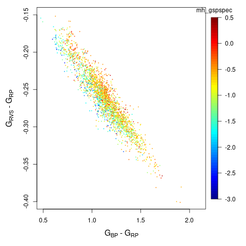
Figure 18: ${\tt grvs\_mag}-G_{\rm RP}$ versus $G_{\rm BP}\ -G_{\rm RP}$ colour–colour diagram for the stars with $V_{\rm tot}>200$ $\text{km\leavevmode\nobreak\ s}^{-1}$in the Milky Way halo (Gaia Collaboration et al., 2018a). The points are colour-coded according to metallicity mh_gspspec as published in DR3 (Recio-Blanco et al., 2022).

8.3 Separating cool dwarfs from cool giants

Figure 19 shows how the ${\tt grvs\_mag}-G_{\rm RP}$ versus $G_{\rm BP}-G_{\rm RP}$ colour–colour relation differs between giants and red dwarfs among low-extinction cool stars, which can help disentangle the two populations. For this figure, all giants ($M_{G}=G+5+5\log(\varpi/1000)>4$ mag) with low extinction ($A_{0}<0.05$, according to Lallement et al. 2019) close to the Galactic plane ($|z|<500$ pc) have been used, while red dwarfs were selected simply with $\varpi>20$ and $M_{G}<4$ mag.

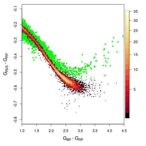
Figure 19: ${\tt grvs\_mag}-G_{\rm RP}$ versus $G_{\rm BP}\ -G_{\rm RP}$ colour–colour diagram for cool stars in DR3. Low-extinction giants are represented with green dots, and nearby cool dwarfs with a red-coloured density plot.

9 Conclusions

We present the DR3 data, methodology, and validation procedure employed to compute the $G_{\rm RVS}$ photometry published in Gaia DR3. The $G_{\rm RVS}$ photometry derived from RVS spectroscopy complements the Gaia photometry derived from astrometric and photometric data. In particular, grvs_mag magnitudes, when combined with standard $G$, $G_{\rm RP}$, and $G_{\rm BP}$ magnitudes, can improve astrophysical information on bright Gaia sources. We show examples of the potential of grvs_mag to constrain interstellar extinction and stellar metallicity and to separate cool dwarfs from cool giants.

The DR3 catalogue contains grvs_mag magnitudes ranging from 2.758 to 14.10 mag for 32.2 million stars with effective temperatures in the range $3100\mathrel{\hbox to0.0pt{\lower 3.5pt\hbox{$\mathchar 536\relax$}\hss}\raise 1.5pt\hbox{$\mathchar 316\relax$}}T_{\rm eff}\mathrel{\hbox to0.0pt{\lower 3.5pt\hbox{$\mathchar 536\relax$}\hss}\raise 1.5pt\hbox{$\mathchar 316\relax$}}14\leavevmode\nobreak\ 500$ K. The median associated uncertainty, grvs_mag_error, ranges from about 0.006 to 0.125 mag from the brightest to the faintest stars. Also listed in the catalogue is the number of epoch observations (or transits), grvs_mag_nbtransits, used to compute grvs_mag. This ranges from 2 to 219, depending on the Gaia scanning law and the density of the observed sky region (the densest regions allowing the fewest exploitable transits). The quantity grvs_mag_nbtransits provides complementary information on the quality of grvs_mag measurements, since fewer transits in general lead to lower-quality data. Combined with grvs_mag_error, it also provides an indication of the dispersion in epoch magnitudes.

The grvs_mag magnitude recorded for each star in the DR3 catalogue is the median of all magnitudes obtained from the epoch observations of that star. The epoch magnitude is measured by integrating the flux in the cleaned RVS spectra, leaving out spectra deemed to be of poor quality, including spectra potentially contaminated by nearby sources and those with saturation issues.

The grvs_mag_error uncertainty associated with grvs_mag is estimated as the formal error on the median, to which an error of 0.004 mag was added in quadrature to account for calibration-floor uncertainties.

To estimate the passband of the effective $G_{\rm RVS}$ filter to which grvs_mag corresponds (over the wavelength range from 846 to 870 nm), the spectra of 108 sources with both high-quality RVS spectra and reference spectra from the CALSPEC and NGSL spectrophotometric libraries were compared. The global RVS transmission derived in this way is better than the pre-launch estimate by a factor of about 1.23. The zero-point of this effective $G_{\rm RVS}$ filter, calibrated based on the reference magnitudes of over $10^{5}$ constant Hipparcos stars, is $ZP=21.317\pm 0.002$ mag.

Gaia DR3 is an intermediate data release based on 34 months of mission data. The next data release will be based on 66 months of data, with a correspondingly higher number of epoch observations and higher S/Ns for the combined data. grvs_mag will be provided for stars fainter than 14.10 mag, and epoch magnitudes will also be published. Other novelties will include the improvement of systematic errors affecting faint stars, and the treatment of crowding.

Appendix A

This work presents results from the European Space Agency (ESA) space mission Gaia. Gaia data are being processed by the Gaia Data Processing and Analysis Consortium (DPAC). Funding for the DPAC is provided by national institutions, in particular the institutions participating in the Gaia MultiLateral Agreement (MLA). The Gaia mission website is https://www.cosmos.esa.int/gaia. The Gaia archive website is https://archives.esac.esa.int/gaia.

The Gaia mission and data processing have financially been supported by, in alphabetical order by country:

• the Algerian Centre de Recherche en Astronomie, Astrophysique et Géophysique of Bouzareah Observatory;

• the Austrian Fonds zur Förderung der wissenschaftlichen Forschung (FWF) Hertha Firnberg Programme through grants T359, P20046, and P23737;

• the BELgian federal Science Policy Office (BELSPO) through various PROgramme de Développement d’Expériences scientifiques (PRODEX) grants and the Polish Academy of Sciences - Fonds Wetenschappelijk Onderzoek through grant VS.091.16N, and the Fonds de la Recherche Scientifique (FNRS), and the Research Council of Katholieke Universiteit (KU) Leuven through grant C16/18/005 (Pushing AsteRoseismology to the next level with TESS, GaiA, and the Sloan DIgital Sky SurvEy – PARADISE);

• the Brazil-France exchange programmes Fundação de Amparo à Pesquisa do Estado de São Paulo (FAPESP) and Coordenação de Aperfeicoamento de Pessoal de Nível Superior (CAPES) - Comité Français d’Evaluation de la Coopération Universitaire et Scientifique avec le Brésil (COFECUB);

• the Chilean Agencia Nacional de Investigación y Desarrollo (ANID) through Fondo Nacional de Desarrollo Científico y Tecnológico (FONDECYT) Regular Project 1210992 (L. Chemin);

• the National Natural Science Foundation of China (NSFC) through grants 11573054, 11703065, and 12173069, the China Scholarship Council through grant 201806040200, and the Natural Science Foundation of Shanghai through grant 21ZR1474100;

• the Tenure Track Pilot Programme of the Croatian Science Foundation and the École Polytechnique Fédérale de Lausanne and the project TTP-2018-07-1171 ‘Mining the Variable Sky’, with the funds of the Croatian-Swiss Research Programme;

• the Czech-Republic Ministry of Education, Youth, and Sports through grant LG 15010 and INTER-EXCELLENCE grant LTAUSA18093, and the Czech Space Office through ESA PECS contract 98058;

• the Danish Ministry of Science;

• the Estonian Ministry of Education and Research through grant IUT40-1;

• the European Commission’s Sixth Framework Programme through the European Leadership in Space Astrometry (ELSA) Marie Curie Research Training Network (MRTN-CT-2006-033481), through Marie Curie project PIOF-GA-2009-255267 (Space AsteroSeismology & RR Lyrae stars, SAS-RRL), and through a Marie Curie Transfer-of-Knowledge (ToK) fellowship (MTKD-CT-2004-014188); the European Commission’s Seventh Framework Programme through grant FP7-606740 (FP7-SPACE-2013-1) for the Gaia European Network for Improved data User Services (GENIUS) and through grant 264895 for the Gaia Research for European Astronomy Training (GREAT-ITN) network;

• the European Cooperation in Science and Technology (COST) through COST Action CA18104 ‘Revealing the Milky Way with Gaia(MW-Gaia)’;

• the European Research Council (ERC) through grants 320360, 647208, and 834148 and through the European Union’s Horizon 2020 research and innovation and excellent science programmes through Marie Skłodowska-Curie grant 745617 (Our Galaxy at full HD – Gal-HD) and 895174 (The build-up and fate of self-gravitating systems in the Universe) as well as grants 687378 (Small Bodies: Near and Far), 682115 (Using the Magellanic Clouds to Understand the Interaction of Galaxies), 695099 (A sub-percent distance scale from binaries and Cepheids – CepBin), 716155 (Structured ACCREtion Disks – SACCRED), 951549 (Sub-percent calibration of the extragalactic distance scale in the era of big surveys – UniverScale), and 101004214 (Innovative Scientific Data Exploration and Exploitation Applications for Space Sciences – EXPLORE);

• the European Science Foundation (ESF), in the framework of the Gaia Research for European Astronomy Training Research Network Programme (GREAT-ESF);

• the European Space Agency (ESA) in the framework of the Gaia project, through the Plan for European Cooperating States (PECS) programme through contracts C98090 and 4000106398/12/NL/KML for Hungary, through contract 4000115263/15/NL/IB for Germany, and through PROgramme de Développement d’Expériences scientifiques (PRODEX) grant 4000127986 for Slovenia;

• the Academy of Finland through grants 299543, 307157, 325805, 328654, 336546, and 345115 and the Magnus Ehrnrooth Foundation;

• the French Centre National d’Études Spatiales (CNES), the Agence Nationale de la Recherche (ANR) through grant ANR-10-IDEX-0001-02 for the ‘Investissements d’avenir’ programme, through grant ANR-15-CE31-0007 for project ‘Modelling the Milky Way in the Gaiaera’ (MOD4Gaia), through grant ANR-14-CE33-0014-01 for project ‘The Milky Way disc formation in the Gaiaera’ (ARCHEOGAL), through grant ANR-15-CE31-0012-01 for project ‘Unlocking the potential of Cepheids as primary distance calibrators’ (UnlockCepheids), through grant ANR-19-CE31-0017 for project ‘Secular evolution of galxies’ (SEGAL), and through grant ANR-18-CE31-0006 for project ‘Galactic Dark Matter’ (GaDaMa), the Centre National de la Recherche Scientifique (CNRS) and its SNO Gaiaof the Institut des Sciences de l’Univers (INSU), its Programmes Nationaux: Cosmologie et Galaxies (PNCG), Gravitation Références Astronomie Métrologie (PNGRAM), Planétologie (PNP), Physique et Chimie du Milieu Interstellaire (PCMI), and Physique Stellaire (PNPS), the ‘Action Fédératrice Gaia’ of the Observatoire de Paris, the Région de Franche-Comté, the Institut National Polytechnique (INP) and the Institut National de Physique nucléaire et de Physique des Particules (IN2P3) co-funded by CNES;

• the German Aerospace Agency (Deutsches Zentrum für Luft- und Raumfahrt e.V., DLR) through grants 50QG0501, 50QG0601, 50QG0602, 50QG0701, 50QG0901, 50QG1001, 50QG1101, 50QG1401, 50QG1402, 50QG1403, 50QG1404, 50QG1904, 50QG2101, 50QG2102, and 50QG2202, and the Centre for Information Services and High Performance Computing (ZIH) at the Technische Universität Dresden for generous allocations of computer time;

• the Hungarian Academy of Sciences through the Lendület Programme grants LP2014-17 and LP2018-7 and the Hungarian National Research, Development, and Innovation Office (NKFIH) through grant KKP-137523 (‘SeismoLab’);

• the Science Foundation Ireland (SFI) through a Royal Society - SFI University Research Fellowship (M. Fraser);

• the Israel Ministry of Science and Technology through grant 3-18143 and the Tel Aviv University Center for Artificial Intelligence and Data Science (TAD) through a grant;

• the Agenzia Spaziale Italiana (ASI) through contracts I/037/08/0, I/058/10/0, 2014-025-R.0, 2014-025-R.1.2015, and 2018-24-HH.0 to the Italian Istituto Nazionale di Astrofisica (INAF), contract 2014-049-R.0/1/2 to INAF for the Space Science Data Centre (SSDC, formerly known as the ASI Science Data Center, ASDC), contracts I/008/10/0, 2013/030/I.0, 2013-030-I.0.1-2015, and 2016-17-I.0 to the Aerospace Logistics Technology Engineering Company (ALTEC S.p.A.), INAF, and the Italian Ministry of Education, University, and Research (Ministero dell’Istruzione, dell’Università e della Ricerca) through the Premiale project ‘MIning The Cosmos Big Data and Innovative Italian Technology for Frontier Astrophysics and Cosmology’ (MITiC);

• the Netherlands Organisation for Scientific Research (NWO) through grant NWO-M-614.061.414, through a VICI grant (A. Helmi), and through a Spinoza prize (A. Helmi), and the Netherlands Research School for Astronomy (NOVA);

• the Polish National Science Centre through HARMONIA grant 2018/30/M/ST9/00311 and DAINA grant 2017/27/L/ST9/03221 and the Ministry of Science and Higher Education (MNiSW) through grant DIR/WK/2018/12;

• the Portuguese Fundação para a Ciência e a Tecnologia (FCT) through national funds, grants SFRH/BD/128840/2017 and PTDC/FIS-AST/30389/2017, and work contract DL 57/2016/CP1364/CT0006, the Fundo Europeu de Desenvolvimento Regional (FEDER) through grant POCI-01-0145-FEDER-030389 and its Programa Operacional Competitividade e Internacionalização (COMPETE2020) through grants UIDB/04434/2020 and UIDP/04434/2020, and the Strategic Programme UIDB/00099/2020 for the Centro de Astrofísica e Gravitação (CENTRA);

• the Slovenian Research Agency through grant P1-0188;

• the Spanish Ministry of Economy (MINECO/FEDER, UE), the Spanish Ministry of Science and Innovation (MICIN), the Spanish Ministry of Education, Culture, and Sports, and the Spanish Government through grants BES-2016-078499, BES-2017-083126, BES-C-2017-0085, ESP2016-80079-C2-1-R, ESP2016-80079-C2-2-R, FPU16/03827, PDC2021-121059-C22, RTI2018-095076-B-C22, and TIN2015-65316-P (‘Computación de Altas Prestaciones VII’), the Juan de la Cierva Incorporación Programme (FJCI-2015-2671 and IJC2019-04862-I for F. Anders), the Severo Ochoa Centre of Excellence Programme (SEV2015-0493), and MICIN/AEI/10.13039/501100011033 (and the European Union through European Regional Development Fund ‘A way of making Europe’) through grant RTI2018-095076-B-C21, the Institute of Cosmos Sciences University of Barcelona (ICCUB, Unidad de Excelencia ‘María de Maeztu’) through grant CEX2019-000918-M, the University of Barcelona’s official doctoral programme for the development of an R+D+i project through an Ajuts de Personal Investigador en Formació (APIF) grant, the Spanish Virtual Observatory through project AyA2017-84089, the Galician Regional Government, Xunta de Galicia, through grants ED431B-2021/36, ED481A-2019/155, and ED481A-2021/296, the Centro de Investigación en Tecnologías de la Información y las Comunicaciones (CITIC), funded by the Xunta de Galicia and the European Union (European Regional Development Fund – Galicia 2014-2020 Programme), through grant ED431G-2019/01, the Red Española de Supercomputación (RES) computer resources at MareNostrum, the Barcelona Supercomputing Centre - Centro Nacional de Supercomputación (BSC-CNS) through activities AECT-2017-2-0002, AECT-2017-3-0006, AECT-2018-1-0017, AECT-2018-2-0013, AECT-2018-3-0011, AECT-2019-1-0010, AECT-2019-2-0014, AECT-2019-3-0003, AECT-2020-1-0004, and DATA-2020-1-0010, the Departament d’Innovació, Universitats i Empresa de la Generalitat de Catalunya through grant 2014-SGR-1051 for project ‘Models de Programació i Entorns d’Execució Parallels’ (MPEXPAR), and Ramon y Cajal Fellowship RYC2018-025968-I funded by MICIN/AEI/10.13039/501100011033 and the European Science Foundation (‘Investing in your future’);

• the Swedish National Space Agency (SNSA/Rymdstyrelsen);

• the Swiss State Secretariat for Education, Research, and Innovation through the Swiss Activités Nationales Complémentaires and the Swiss National Science Foundation through an Eccellenza Professorial Fellowship (award PCEFP2_194638 for R. Anderson);

• the United Kingdom Particle Physics and Astronomy Research Council (PPARC), the United Kingdom Science and Technology Facilities Council (STFC), and the United Kingdom Space Agency (UKSA) through the following grants to the University of Bristol, the University of Cambridge, the University of Edinburgh, the University of Leicester, the Mullard Space Sciences Laboratory of University College London, and the United Kingdom Rutherford Appleton Laboratory (RAL): PP/D006511/1, PP/D006546/1, PP/D006570/1, ST/I000852/1, ST/J005045/1, ST/K00056X/1, ST/K000209/1, ST/K000756/1, ST/L006561/1, ST/N000595/1, ST/N000641/1, ST/N000978/1, ST/N001117/1, ST/S000089/1, ST/S000976/1, ST/S000984/1, ST/S001123/1, ST/S001948/1, ST/S001980/1, ST/S002103/1, ST/V000969/1, ST/W002469/1, ST/W002493/1, ST/W002671/1, ST/W002809/1, and EP/V520342/1.

The GBOT programme uses observations collected at (i) the European Organisation for Astronomical Research in the Southern Hemisphere (ESO) with the VLT Survey Telescope (VST), under ESO programmes 092.B-0165, 093.B-0236, 094.B-0181, 095.B-0046, 096.B-0162, 097.B-0304, 098.B-0030, 099.B-0034, 0100.B-0131, 0101.B-0156, 0102.B-0174, and 0103.B-0165; and (ii) the Liverpool Telescope, which is operated on the island of La Palma by Liverpool John Moores University in the Spanish Observatorio del Roque de los Muchachos of the Instituto de Astrofísica de Canarias with financial support from the United Kingdom Science and Technology Facilities Council, and (iii) telescopes of the Las Cumbres Observatory Global Telescope Network. AMB acknowledges funding from the European Union’s Horizon 2020 research and innovation programme under the Marie Skłodowska-Curie grant agreement No 895174. We made use of TOPCAT: http://www.starlink.ac.uk/topcat.

References

- Ahumada et al. (2020) Ahumada, R., Prieto, C. A., Almeida, A., et al. 2020, ApJS, 249, 3
- Andrae et al. (2022) Andrae, R., Fouesneau, M., Sordo, R., et al. 2022, A&A submitted.
- Babusiaux et al. (2022) Babusiaux, C., Fabricius, C., Khanna, S., Muraveva, T., & et al. 2022, submitted to A&A
- Blomme et al. (2022) Blomme, R., Fremat, Y., Sartoretti, P., et al. 2022, submitted to A&A
- Bohlin et al. (2014) Bohlin, R. C., Gordon, K. D., & Tremblay, P. E. 2014, PASP, 126, 711
- Bonifacio et al. (2018) Bonifacio, P., Caffau, E., Ludwig, H. G., et al. 2018, A&A, 611, A68
- Bovy et al. (2014) Bovy, J., Nidever, D. L., Rix, H.-W., et al. 2014, ApJ, 790, 127
- Cropper et al. (2018) Cropper, M., Katz, D., Sartoretti, P., et al. 2018, A&A, 616, A5
- Damerdji & et al. (2022) Damerdji, Y. & et al. 2022, A&A in prep.
- Fabricius et al. (2021) Fabricius, C., Luri, X., Arenou, F., et al. 2021, A&A, 649, A5
- Fitzpatrick et al. (2019) Fitzpatrick, E. L., Massa, D., Gordon, K. D., Bohlin, R., & Clayton, G. C. 2019, ApJ, 886, 108
- Fremat et al. (2022) Fremat, Y., Royer, F., Marchal, O., et al. 2022, submitted to A&A
- Gaia Collaboration et al. (2018a) Gaia Collaboration, Babusiaux, C., van Leeuwen, F., et al. 2018a, A&A, 616, A10
- Gaia Collaboration et al. (2018b) Gaia Collaboration, Brown, A. G. A., Vallenari, A., et al. 2018b, A&A, 616, A1
- Gaia Collaboration et al. (2021) Gaia Collaboration, Brown, A. G. A., Vallenari, A., et al. 2021, A&A, 649, A1
- Gaia Collaboration et al. (2016) Gaia Collaboration, Prusti, T., de Bruijne, J., Brown, A., & et al. 2016, A&A, 595, A1
- Gaia Collaboration et al. (2022) Gaia Collaboration, Vallenari, A., & et al. 2022, A&A in prep.
- Hambly et al. (2018) Hambly, N. C., Cropper, M., Boudreault, S., et al. 2018, A&A, 616, A15
- Heap & Lindler (2016) Heap, S. R. & Lindler, D. 2016, in Astronomical Society of the Pacific Conference Series, Vol. 503, The Science of Calibration, ed. S. Deustua, S. Allam, D. Tucker, & J. A. Smith, 211
- Høg et al. (2000) Høg, E., Fabricius, C., Makarov, V. V., et al. 2000, A&A, 355, L27
- Horne (1986) Horne, K. 1986, PASP, 98, 609
- Jordi et al. (2010) Jordi, C., Gebran, M., Carrasco, J. M., et al. 2010, A&A, 523, A48
- Katz et al. (2022) Katz, D., Sartoretti, P., Guerrier, A., et al. 2022, A&A in prep.
- Lallement et al. (2019) Lallement, R., Babusiaux, C., Vergely, J. L., et al. 2019, A&A, 625, A135
- Montegriffo et al. (2022) Montegriffo, P., De Angeli, F., Andrae, R., et al. 2022, submitted to A&A
- Ng & Maechler (2007) Ng, P. & Maechler, M. 2007, Statistical Modelling: An International Journal, 7, 315
- Perryman et al. (1997) Perryman, M. A. C., Lindegren, L., Kovalevsky, J., et al. 1997, A&A, 323, L49
- Recio-Blanco et al. (2022) Recio-Blanco, A., de Laverny, P., Palicio, P. A., et al. 2022, submitted to A&A
- Riello et al. (2021) Riello, M., De Angeli, F., Evans, D. W., et al. 2021, A&A, 649, A3
- Sartoretti et al. (2022) Sartoretti, P., Blomme, R., David, M., & Seabroke, G. 2022, Gaia DR3 documentation Chapter 6: Spectroscopy, Gaia DR3 documentation
- Sartoretti et al. (2018) Sartoretti, P., Katz, D., Cropper, M., et al. 2018, A&A, 616, A6
- Seabroke & et al. (2022) Seabroke, G. & et al. 2022, A&A in prep.
- Seabroke et al. (2021) Seabroke, G. M., Fabricius, C., Teyssier, D., et al. 2021, A&A, 653, A160