smoothEM: a new approach for the simultaneous assessment of smooth patterns and spikes

Abstract

We consider functional data where an underlying smooth curve is composed not just with errors, but also with irregular spikes. We propose an approach that, combining regularized spline smoothing and an Expectation-Maximization (EM) algorithm, allows one to both identify spikes and estimate the smooth component. Imposing some assumptions on the error distribution, we prove consistency of EM estimates. Next, we demonstrate the performance of our proposal on finite samples and its robustness to assumptions violations through simulations. Finally, we apply our proposal to data on the annual heatwaves index in the US and on weekly electricity consumption in Ireland. In both data sets, we are able to characterize underlying smooth trends and to pinpoint irregular/extreme behaviors.

Keywords: functional data analysis, penalized smoothing, EM algorithm

1 Introduction and Motivation

The past two decades have witnessed an increasing interest in functional data, where one or more variables are data varying over a continuum and often possessing additional structures of interest. The vast majority of past and current literature focuses on functional data obeying certain smoothness conditions (see, e.g., Ramsay & Silverman, 2007; Kokoszka & Reimherr, 2017), which can be effectively represented in low dimension through basis functions (e.g., Fourier basis, spline basis or polynomial basis). In the majority of applications, a penalty is employed to ensure such representation – an approach commonly referred to as penalized/regularized smoothing (Yao & Lee, 2006; Goldsmith et al., 2011).

Real-world data often contain, on top of underlying smooth trends, sporadic discontinuities that can be interesting in and of themselves. Meaningful examples include data on extreme temperatures and electricity consumption, to name a few. As we shall see later, in both cases one can observe discontinuous spikes occurring on top of smooth underlying trends, due, e.g., to sporadic abnormalities in weather conditions or occasional over-consumption of electricity. For these discontinuous data, a simple application of penalized smoothing that does not account for the spikes can generate an inaccurate approximation of the underlying curve. In this article, we seek to produce reliable estimates of the underlying trends and identify the spikes simultaneously, the latter of which can be analyzed to gain insight into their frequency, location, magnitude and spread.

In existing literature, wavelet representation is often used to handle discontinuities due to its multi-scale nature and ability to adapt to local features in the data (Nason, 2008). However, wavelet representation often suffers from boundary effects and does not present an intuitive way to incorporate smoothness information of the underlying trend. Another approach is provided by Descary & Panaretos (2019), who consider functions with rough components that are assumed smooth at local scales. More specifically, these authors consider functions expressed as the sum of two uncorrelated components, $X(t)=Y(t)+W(t)$, where $Y(t)$ is taken to be of finite rank and of smoothness class $C^{k}$ ($k\geq 2)$, and $W(t)$ is locally highly variable but continuous at a shorter time scale. While interesting, this set-up is only an approximation for functions that contain true discontinuities, and are thus non-smooth at any scale. Another possible candidate is adaptive smoothing (Luo & Wahba, 1997; Pintore et al., 2006), whose adaptive nature might be useful for increasing the local penalty where there are discontinuities, thus reducing their influence. However, by nature of their objective functions, adaptive smoothing methods tend to do the opposite: they decrease the local penalty to accommodate discontinuities, thus making the estimated smooth component even more wiggly. On a separate front, the field of spectroscopic analysis has produced several baseline correction methods to treat signals (e.g., raw Raman spectra or standard chromatograms) consisting of a smooth baseline with occasional positive spikes – which are not of interest and are treated as contamination to be eliminated. Many of these methods employ iterative penalized smoothing, with adaptive weights informed by the sign and magnitude of residuals (Wei et al., 2022; Zhang et al., 2010). While of great interest, these methods are generally limited to simple and slowly varying smooth baselines, and are therefore ineffective when more complex smooth structures exist. In this article, we propose a novel framework that represents discontinuities explicitly. Broad distributional assumptions about the data allow us to exploit both the magnitude and the variance of the spikes, and to simultaneously perform smooth curve estimation and spike identification. In symbols, we are interested in data $(x_{i},y_{i})_{i=1}^{n}$ of the form

$$y_{i}=f(x_{i})+\mu^{*}\cdot\mathbbm{1}(x_{i}\in\mathbb{S})+\epsilon_{i}$$ (1)

where $x_{i}$, $i=1\ldots,n$ are locations in a domain (which we map in $[0,1]$ without loss of generality); $f\in C^{p}[0,1]$ is a smooth function with $p$ continuous derivatives; $\mathbb{S}$ is a random collection of intervals on $[0,1]$ affected by spikes of size $\mu^{*}$ such that $\mathbb{S}$ has probability measure $1-\alpha^{*}$; $\mathbbm{1}(x_{i}\in\mathbb{S})$, $i=1\ldots,n$ is an indicator of spike occurrences; and $\epsilon_{i}$, $i=1\ldots,n$ are independent random errors. Assuming a fixed design, our main goal is to capture the underlying curve and to identify the spikes, i.e. to estimate $f$ and the spike classification vector $\mathbbm{1}_{\mathbb{S}}=(\mathbbm{1}(x_{i}\in\mathbb{S}))_{i=1}^{n}$.

With the additional assumption that errors are Gaussian, we rewrite Equation (1) as $y_{i}=f(x_{i})+\xi_{i}$, where $\xi_{i}:=\mu^{*}\cdot\mathbbm{1}(x_{i}\in\mathbb{S})+\epsilon_{i}$ can be modeled as a mixture of Gaussians:

$$\xi_{i}\sim\alpha^{*}N(0,\sigma^{*2})+(1-\alpha^{*})N(\mu^{*},\sigma^{*2}).$$ (2)

Thus, with probability $\alpha^{*}\in(0.5,1)$, the departure from $f$ is Gaussian with mean $0$ and variance $\sigma^{*2}$, but with probability $(1-\alpha^{*})$ it is “spiked” by a scalar amount $\mu^{*}$. Equation (2) can be extended to accommodate size-varying spikes as

$$\xi_{i}\sim\alpha^{*}N(0,\sigma^{*2})+(1-\alpha^{*})N(\mu^{*},\sigma^{*2}+\sigma_{h}^{*2}).$$ (3)

We deal with size-varying spikes in Section 5. Here we focus attention on the model in Equation 2. In this setting, maximum likelihood estimates (MLE) of $\alpha^{*},\mu^{*}$ and $\sigma^{*}$ could be obtained through the Expectation-Maximization (EM) algorithm if the $\xi_{i}$’s were observable. Previous work on EM convergence often assumed that the only parameter to be estimated is $\mu^{*}$, with both $\sigma^{*2}$ and $\alpha^{*}$ taken as known; see for instance (Wu et al., 2017) and (Balakrishnan et al., 2017). Drawing inspiration from the latter, we study convergence when all parameters $\mu^{*},\sigma^{*2}$ and $\alpha^{*}$ are unknown – proving that $\nu-$strong concavity, Lipschitz smoothness and Gradient smoothness conditions hold for our Gaussian mixture model. In such a case, guarantees on the convergence rate are harder to establish, but can in fact be provided if the “contamination” level $\alpha^{*}$ is taken as known. We use simulations to demonstrate the practical effectiveness of our approach notwithstanding this shortcoming in theoretical guarantees.

The remainder of this article is organized as follows. Section 2 provides background on smoothing splines and EM algorithm. Section 3 details our approach and the conditions under which it performs well. Section 4 provides convergence guarantees for the EM algorithm. Sections 5 and 6 demonstrate the performance of our proposal through simulations, comparisons with existing methods and real data analyses. Section 7 contains final remarks.

2 Technical background

2.1 Penalized smoothing splines

Suppose that the data $(x_{i},y_{i})_{i=1}^{n}$ are generated according to

$$y_{i}=f(x_{i})+\epsilon_{i}$$ (4)

where $x_{i}\in[0,1],i=1,\ldots n$ are either fixed or random, and the $\epsilon_{i}$’s represent white noise (independent and Gaussian random errors). Assuming that $f$ has $p$ continuous derivatives on $[0,1]$, i.e. that $f\in C^{p}[0,1]$, it is often of interest to approximate $f$ from $(x_{i},y_{i})_{i=1}^{n}$. In a spline approximation (de Boor, 1978; Xiao, 2019) the estimator $\hat{f}$ is restricted to lie in the space of spline functions of order $m$. Functions in this space have the representation $\sum_{k}a_{k}N_{k}(x)$ where $N_{k}(x)$ is the $k^{th}$ B-spline function. Depending on the number of basis functions $\hat{f}$ can either underfit or overfit the data. To prevent this, $\hat{f}$ is regularized by placing a penalty on its higher-order derivatives (see, e.g., O’Sullivan, 1986; Ramsay & Silverman, 2007; Xiao, 2019); that is, to minimize

$$\sum_{i=1}^{n}\bigg{\{}y_{i}-\sum_{k=1}^{K}a_{k}N_{k}(x_{i})\bigg{\}}^{2}+\lambda\int_{0}^{1}\bigg{\{}\sum_{k=1}^{K}a_{k}N_{k}^{(q)}(x)\bigg{\}}^{2}dx$$ (5)

where $\lambda$ is a tuning parameter whose optimal value can be found using cross validation. Equation (5) has a vectorized representation

$$\min_{\boldsymbol{a}}\bigg{(}\frac{1}{n}\left\|y-Na\right\|_{2}^{2}+\lambda a^{\top}P_{q}a\bigg{)}$$ (6)

where $y=(y_{1},\ldots,y_{n})^{\top}$, $N=(N_{1}(x),\ldots,N_{K}(x))^{\top}$, $a=(a_{1},\ldots,a_{K})^{\top}$ are column vectors and $P_{q}$ is the penalization matrix. The explicit form of $P_{q}$ is not needed for the purposes of this article; interested readers can find more details in Xiao (2019). Equation (6) can be solved explicitly; indeed, if we set $H_{n}:=N^{\top}N/n+\lambda P_{q}$, then the solutions are

$$\hat{a}=H_{n}^{-1}(N^{\top}y/n),\ \ \hat{f}(x)=N^{\top}(x)H_{n}^{-1}(N^{\top}y/n).$$

2.2 EM algorithm for Gaussian mixtures

Let $\xi\in\Xi$ and $z\in Z$ be random variables whose joint density function is $\phi_{\theta^{*}}$, where $\theta^{*}$ belongs to a (non-empty) convex parameter space $\Omega$. Suppose we can observe data $(\xi_{i})_{i=1}^{n}$, while the $(z_{i})_{i=1}^{n}$ are unobservable, and that $(\xi_{i}|z_{i}=j)\overset{iid}{\sim}G_{j}$ where the $G_{j}$’s are Gaussian distributions. Our goal is to estimate the unknown $\theta^{*}$ using Maximum Likelihood; that is, to find $\hat{\theta}$ that maximizes

$$\ell_{n}(\theta)=\frac{1}{n}\sum_{i=1}^{n}\log\bigg{(}\int_{Z}\phi_{\theta}(\xi_{i},z_{i})dz_{i}\bigg{)}\ .$$

In practice, the function $\ell_{n}$ is usually hard to optimize. The EM algorithm provides a way of searching for such maximum indirectly through the maximization of another function $Q_{n}:\Omega\times\Omega\rightarrow\mathbb{R}$ defined as

$$Q_{n}(\theta|\theta^{\prime})=\frac{1}{n}\sum_{i=1}^{n}\bigg{(}\int_{Z}k_{\theta^{\prime}}(z|\xi_{i})\log\phi_{\theta}(\xi_{i},z)dz\bigg{)}$$

where $k_{\theta^{\prime}}(z|\xi)$ is the conditional density of $z$ given $\xi$. Given this function and a current estimate $\theta_{n,t}$, the sample EM update is defined as

$$\theta_{n,t+1}=\theta_{n,t}+s\nabla Q_{n}(\theta|\theta_{n,t})\big{|}_{\theta=\theta_{n,t}},\qquad t=0,1,\ldots\ .$$

where $s$ is the step size. To study convergence of the EM to a (neighborhood of) the global optimum, Balakrishnan et al. (2017) define the population level versions $\ell$ of $\ell_{n}$ and $Q$ of $Q_{n}$ as

$$\ell(\theta)= \ \int_{\Xi}log\bigg{(}\int_{Z}\phi_{\theta}(\xi_{i},z_{i})dz_{i}\bigg{)}g_{\theta^{*}}(\xi)d\xi$$

$$Q(\theta|\theta^{\prime})= \ \int_{\xi}\bigg{(}\int_{Z}k_{\theta^{\prime}}(z|\xi_{i})\log\phi_{\theta}(\xi_{i},z)dz\bigg{)}g_{\theta^{*}}(\xi)d\xi\ .$$

Correspondingly, one has a population version of the EM update

$$\theta_{t+1}=\theta_{t}+s\nabla Q(\theta|\theta_{t})\big{|}_{\theta=\theta_{t}},\qquad t=0,1,\ldots\ .$$

Based on this, since $\theta^{*}$ maximizes $\ell(\theta)$, to prove that the sample EM update converges to (a neighborhood of) $\theta^{*}$, one needs to prove that (i) the population EM update converges to (a neighborhood of) $\theta^{*}$; and (ii) the sample EM update tracks closely the population update (this is precisely what we do in Theorem 1 and Theorem 2 below).

3 The smoothEM approach

Let us consider again data as in Equations (1) and (2); that is

$$\xi_{i} :=y_{i}-f(x_{i})=\begin{cases}\mu^{*}+\epsilon_{i},\text{ if }x_{i}\in\mathbb{S}\\ \epsilon_{i},\text{ otherwise}\end{cases}$$

$$\sim\alpha^{*}N(0,\sigma^{*2})+(1-\alpha^{*})N(\mu^{*},\sigma^{*2})$$

where the design (the $x_{i}$’s) is taken as fixed. If we knew $f$, the EM algorithm could be used to search for the MLE of the mixture parameters $\theta^{*}=(\alpha^{*},\mu^{*},\sigma^{*2})$ and to estimate membership (i.e. posterior) probabilities for each point, and thus the classification vector $\mathbbm{1}_{\mathbb{S}}$. In reality, we do not know $f$, so we use the EM with an estimate $\hat{f}$ of $f$. The traditional penalized smoothing technique in Equation (5) is ill-fitted for the above purpose. Indeed, it declares as optimal an $\hat{f}$ that minimizes a combination of sum of squared errors and degree of roughness. The tuning parameter $\lambda$, generally chosen by cross validation, determines the balance between these two competing criteria. In the case of noisy curves with spikes as defined in Equation (1), a sufficiently large $\mu^{*}$ causes the sum of squared errors term to dominate the roughness criterion. This in turns causes the cross validation procedure to be biased towards small values of $\lambda$, i.e. towards under-smoothed $\hat{f}$. This is the key observation that gives rise to our iterated penalized smoothing procedure, which we illustrate through two simple examples.

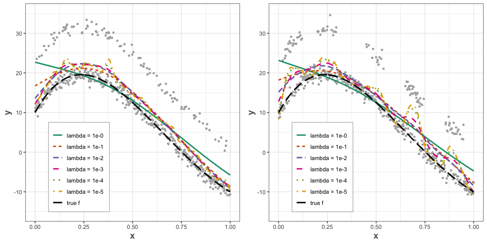
Figure 1: Simulated data and smoothing spline fit for $f$ with different values of the tuning parameter $\lambda$ (curves of different types and colors). The dashed black curve represents the true $f$. Left: independently and uniformly distributed spikes. Right: spikes clustered into “hovering clouds”.

Figure 1 plots $n=500$ data points simulated across the $[0,1]$ domain. The majority of such points are scattered about a fourth degree polynomial, the curve $f$, with independent errors $\epsilon_{i}\sim N(0,1)$. In the left panel, spikes occur uniformly across the domain and independently from other data points, while in the right panel, spikes form “hovering clouds” of different denseness at different locations along the domain. In both scenarios, spikes are shifted vertically by $\mu^{*}=12$. We note that the clustered spikes (right panel) are correlated, and thus represent a departure from our assumed mixture Gaussian model. Even if our theoretical results require independence, we show with simulations in Section 5 that our algorithm is robust to this departure from the theoretical assumptions, maintaining its ability to identify spikes and recover the true $f$ also in this case. The true $f$ is plotted in black, and the estimates $\hat{f}$, obtained through 300 cubic spline basis functions with equally spaced knots and penalty of order 1, are plotted in different colors depending on the values of $\lambda$. At first glance, none of the $\hat{f}$’s approximates $f$ well, though some give better fits than others. In particular, the presence of spikes, especially when coupled with larger $\lambda$, affects estimation at both spike and non-spike locations. Also, for the correlated case (right panel), “denser” spikes sites distort $\hat{f}$ to a higher degree – especially for small $\lambda$ values. Generalized cross-validation here selects $\lambda=10^{-4}$, which still results in a highly distorted $\hat{f}$. Suppose now we were to identify spikes and do inference on the parameters $\alpha^{*},\mu^{*},\sigma^{*2}$ through the residuals from $\hat{f}$. Such a distorted estimate would generate misleading residuals. On the other hand, just from visual inspection, $\lambda=10^{-1}$ and $\lambda=10^{-2}$ produce much more reasonable $\hat{f}$’s and, correspondingly, residuals which are a much better approximation of the underlying $\xi_{i}$’s, giving some hope that one may be able to identify spikes based on their magnitudes. If we identify and filter out the spikes, and then repeat regularized smoothing, we can obtain a much improved fit to $f$.

3.1 smoothEM: the algorithm

Based on the above reasoning, we propose our smoothEM procedure, which comprises the following steps:

1. Fit penalized smoothing splines over a grid of $\lambda$’s and obtain residuals $\xi_{\lambda}=\{\xi_{i}(\lambda)\}_{i=1}^{n}$.

2. For each pair $(\lambda,\xi_{\lambda})$, classify as “spikes” the set of largest $\xi_{i}(\lambda)$’s (with a bound on its cardinality, e.g., $\leq 50\%$ of the observations), thus producing binary memberships $M_{\lambda}=\{M_{i}(\lambda)\}_{i=1}^{n}$ ($M_{i}(\lambda)=0,1$ if $i$ is classified as “smooth” or “spike”, respectively).

3. For each pair $(\lambda,M_{\lambda})$, fit a second penalized smoothing spline using only observations with $M_{i}(\lambda)=0$, and compute updated residuals $\xi^{\prime}_{\lambda}$ for all observations. Here we also compute an “overfit” score $F(\lambda)$ based on how much the fit $\hat{f}$ changes when smooth observations ($M_{i}(\lambda)=0$) are perturbed by a small amount (see below).

4. For each $\lambda$, run the EM algorithm on $\xi^{\prime}_{\lambda}$ with $M_{\lambda}$ as initialization, to produce parameter estimates $(\hat{\alpha},\hat{\mu},\hat{\sigma}^{2})_{\lambda}$ and new memberships $M^{\prime}_{\lambda}$, obtained by thresholding posterior probabilities (our implementation automatically selects the threshold between 0.5 and 1 such that the classification maximizes the log-likelihood).

5. Considering a combination of log-likelihood and “overfit” scores, select $\lambda^{*}=\arg\max_{\lambda}\allowbreak\left[\ell(\lambda;\hat{\alpha},\hat{\mu},\hat{\sigma}^{2})+F(\lambda)\right]$ and thus parameter estimates $(\hat{\alpha},\hat{\mu},\hat{\sigma}^{2})_{\lambda^{*}}$ and memberships $M^{\prime}_{\lambda^{*}}$.

6. Refit a penalized smoothing spline with $\lambda=\lambda^{*}$, using only observations that satisfy $M^{\prime}_{i}(\lambda^{*})=0$.

3.2 Some observations and remarks

The performance of our procedure depends critically on the grid of $\lambda$ values chosen for its implementation. A relatively small grid suffices if one has prior knowledge about the smoothness of $f$. Otherwise, we recommend exploring a dense grid, likely to include a good $\lambda$ value , withstanding the greater computational cost. Also, the initial residual magnitude-based classification in Step 2 can be implemented in different ways, with different computational costs (e.g., running a 1-dimensional $K$-means, or pinpointing the largest difference in the ordered sequence).

In our experience, the overfit score $F$ in Step 3 is especially helpful when there is a limited number of observations. Without it, the algorithm might favor very small values of $\lambda$ and overfit most/all observations, leading to near zero residuals (almost) everywhere and producing very high likelihood values in later steps. The overfit score $F$ is calculated as follows. Let $\xi$ be the collection of residuals and $\xi^{(0)}$ the sub-collection corresponding to “smooth” observations ($M_{i}=0$). Let $\xi_{p}^{(0)}$ be a perturbed version of $\xi^{(0)}$ obtained as $\xi_{p}^{(0)}=\xi^{(0)}+\tau$, where $\tau$ is a vector of independent variables from a $N(0,\sigma^{2}_{\tau})$. Let $\hat{f}(\xi^{(0)})$ and $\hat{f}(\xi_{p}^{(0)})$ be the curves fitted to $\xi^{(0)}$ and $\xi_{p}^{(0)}$, respectively, and compute the score as $F=\small\|\hat{f}(\xi^{(0)})-\hat{f}(\xi_{p}^{(0)})\small\|_{2}$. Here, the amount of perturbation can be chosen to match the overall level of noise in the original data. We recommend using a robust estimation of standard deviation, e.g., $\sigma_{\tau}=median(|\hat{\xi}_{i}-median(\hat{\xi})|)$, where $\hat{\xi}$ are rough residual estimates obtained from fitting a loess curve to the raw data.

An R implementation of smoothEM and some examples are provided at https://github.com/hqd1/smoothEM

4 Theoretical remarks and guarantees

4.1 Remarks for iterated smoothing

Here we discuss in more detail the interplay between the smoothness of $f$, $\lambda$, $\mu^{*}/\sigma^{*}$, $n$, and the denseness of spikes, in determining the effectiveness of iterated smoothing. We assume that $(x_{i},y_{i})_{i=1}^{n}$ are generated as at the beginning of Section 3, but the remarks in this subsection also extend to the case of correlated spikes. For a given realization of $\mathbbm{1}(x_{i}\in\mathbb{S})$ (i.e. with spike locations fixed), the only randomness is from $(\epsilon_{i})_{i=1}^{n}$. Assuming without loss of generality that $\mu^{*}>0$, let $r(x_{p})$ and $r(x_{s})$ be residuals from Step 1 at spike location $x_{p}$ and smooth location $x_{s}$. The difference

$$r(x_{p})-r(x_{s}) =y_{p}-\hat{f}(x_{p})-(y_{s}-\hat{f}(x_{s}))$$

$$=f(x_{p})+\mu^{*}+\epsilon_{p}-N(x_{p})H^{-1}_{n}N^{\top}(f(x)+\mu^{*}\cdot\mathbbm{1}_{\mathbb{S}}+\epsilon)/n$$

$$\quad-[f(x_{s})+\epsilon_{s}-N(x_{s})H^{-1}_{n}N^{\top}(f(x)+\mu^{*}\cdot\mathbbm{1}_{\mathbb{S}}+\epsilon)/n]$$

(see Section 2.1) can be decomposed as $r(x_{p})-r(x_{s})=R_{1}+R_{2}+R_{3}$, where

$$R_{1}=f(x_{p})-N(x_{p})H^{-1}_{n}N^{\top}(f(x)+\epsilon)/n-[f(x_{s})-N(x_{s})H^{-1}_{n}N^{\top}(f(x)+\epsilon)/n],$$

$$R_{2}=\mu^{*}-N(x_{p})H^{-1}_{n}N^{\top}\mu^{*}\cdot\mathbbm{1}_{\mathbb{S}}/n-[0-N(x_{s})H^{-1}_{n}N^{\top}\mu^{*}\cdot\mathbbm{1}_{\mathbb{S}}/n],$$

$$R_{3}=\epsilon_{p}-\epsilon_{s}.$$

The first component is $R_{1}=r^{\prime}(x_{p})-r^{\prime}(x_{s})$, the difference of the residuals from fitting a spline to the noisy curve only. As long as the underlying true $f(x)$ is $\in C^{p}[0,1]$ for $p\leq m$, where $m$ is the order of the smoothing spline, Xiao (2019) guarantees that under appropriate conditions $\max_{x}r^{\prime}(x)$ is of order $o\left\{\left(\log{n}/n\right)^{-m/(2m+1)}\right\}$. The second component is $R_{2}=r^{\prime\prime}(x_{p})-r^{\prime\prime}(x_{s})$, the difference of the residuals from fitting a spline to the $n$-discretized piecewise constant $\mu^{*}\cdot\mathbbm{1}_{\mathbb{S}}$. As spline smoothing is highly localized by nature, intuitively, if the number of spikes in a neighborhood of $x_{p}$ is sufficiently small and $\lambda$ is sufficiently large, the smoothing spline will prioritize approximation of the constant line $g(\cdot)=0$, causing $r^{\prime\prime}(x_{p})-r^{\prime\prime}(x_{s})$ to be near $\mu^{*}$. As more spikes gather around $x_{p}$, this magnitude decreases, making spikes less distinguishable. It is important to note that the same $\lambda$ is used to fit the noisy curve in $R_{1}$ and $\mu^{*}\cdot\mathbbm{1}_{\mathbb{S}}$ in $R_{2}$. As a consequence, if $f(x)$ is rather jagged and thus the optimal $\lambda$ to fit it is small, one may easily overfit $\mu^{*}\cdot\mathbbm{1}_{\mathbb{S}}$ – especially when spikes are dense in a neighborhood of $x_{p}$. The third component is simply $R_{3}=\epsilon_{p}-\epsilon_{s}$. Under ideal conditions, $R_{1}$ will be close to 0, $R_{2}$ will be close to $\mu^{*}$, and as long as $\mu^{*}/\sigma^{*2}$ is large, the effect of $R_{3}$ will be negligible.

4.2 Results for EM

In the following, let $q(\theta)=Q(\theta|\theta^{*})$ (see Section 2.2), $\omega$ is an arbitrarily small, positive number, and let $\mathbb{B}_{2}(r;\theta^{*})$ denote an $L_{2}$ ball centered at $\theta^{*}$ with radius $r$.

Theorem 1 (Population level guarantees for the Gaussian mixture model)

Consider the Gaussian mixture model in Equation (2) with unknown parameters $\theta^{*}=(\alpha^{*},\mu^{*},\sigma^{*2})\in(0.5,1)\times\mathbb{R}\times\mathbb{R}^{+}$. Given any initialization $\theta_{0}\in\mathbb{B}_{2}(r;\theta^{*})$, the population first order EM iterates satisfy the bound

$$\left\|\theta_{k}-\theta^{*}\right\|_{2}\leq\bigg{(}1-\frac{2\nu-\gamma}{L+\nu}\bigg{)}^{k}\left\|\theta_{0}-\theta^{*}\right\|_{2}\quad\text{ for all }k=1,2,\ldots$$

where $0\leq\gamma<\nu\leq L$ and

• $\nu=\min\left\{\left(\frac{1}{(\alpha^{*}+r)^{2}}\vee 1\right),\frac{\sigma^{*2}-r}{2(\sigma^{*2}+r)^{3}}-\frac{(1-\alpha^{*})r}{(\sigma^{*2}-r)^{2}},\frac{1-\alpha^{*}}{\sigma^{*2}+r}-\frac{(1-\alpha^{*})r}{(\sigma^{*2}-r)^{2}}\right\}$;

• $L=\max\left\{\frac{\alpha^{*}}{(\alpha^{*}-r\ \vee\ 0.5)^{2}}+\frac{1-\alpha^{*}}{(1-\alpha^{*}-r\ \vee\ \omega)^{2}},\frac{(1-\alpha^{*})\sigma^{*2}}{(\sigma^{*2}-r)^{2}},\frac{\sigma^{*2}+r}{2(\sigma^{*2}-r)^{3}}+\frac{1-\alpha^{*}}{\sigma^{*2}-r}\right\}$;

• $\gamma(\alpha^{*},\mu^{*},\sigma^{*2})\sim O\left(\frac{\mu^{*5}}{\sigma^{*8}}\exp(-\frac{\mu^{*}-r}{\sigma^{*2}+r})\right)$, which decays exponentially with large $\frac{\mu^{*}}{\sigma^{*2}}$.

Before proceeding, some remarks are in order on the use of Theorem 1. First, Balakrishnan et al. (2017) proved exponential convergence rate for the same model, but assuming known $\alpha^{*}$ and $\sigma^{*2}$. Such exponential rate is achievable because, if $\alpha^{*}$ and $\sigma^{*2}$ are known, $\nu=L$ and $\left[1-\left(2\nu-\gamma\right)/\left(L+\nu\right)\right]$ is reduced to just $\gamma/(2L)$. Theorem 1 provides a slower convergence rate, but considers all parameters as unknown (a proof is provided in the Supplementary Material).

Second, $\nu$ decreases as $r$ increases; this creates an undesirable trade off, as ideally we would want both to be large. A larger $r$ allows for a larger basin of attraction for convergence but slows convergence, whereas a larger $\nu$ hastens the convergence rate. Choosing $r=\sigma^{*2}/5$ ensures that $\nu>0$.

Third, even with a positive $\nu$, the convergence rate can be slowed by a large Lipschitz smoothness constant $L$. In particular, an arbitrarily large $(1-\alpha^{*})/(1-\alpha^{*}-r\ \vee\ \omega)^{2}$ makes the rate $\left[1-\left(2\nu-\gamma\right)/\left(L+\nu\right)\right]^{k}$ unacceptably slow. A workaround is to require that $\alpha_{0}\in\mathbb{B}_{2}(r_{\alpha};\alpha^{*})$, where $r_{\alpha}<r$ is a small constant, so that $L$ is bounded by $(1-\alpha^{*})/(1-\alpha^{*}-r_{\alpha})^{2}$ instead. As an example, a reasonable choice for $r_{\alpha}$ is $0.25-\alpha^{*}/4$.

Table 1: Convergence rate $CR=\left[1-(2\nu-\gamma)/(L+\nu)\right]$ for different values of $\alpha^{*}$, $\sigma^{*2}$, and $r=\sigma^{*2}/5$. Rates are calculated assuming a sufficiently large signal to noise ratio $\mu^{*}/\sigma^{*2}$.

$CR$ $(\sigma^{*2},r)$ (1, 0.2) (2, 0.4) (3, 0.6) (4, 0.8) (5, 1) .6 0.932 0.969 0.979 0.985 0.988 .7 0.957 0.979 0.986 0.989 0.992 .8 0.966 0.989 0.993 0.995 0.996 $\alpha^{*}$ .9 0.979 0.996 0.998 0.999 0.999

Table 1 provides the convergence rates for various parameter settings, assuming sufficiently large signal to noise ratio $\mu^{*}/\sigma^{*2}$. As to be expected, convergence rates improve with lower noise levels and more balanced proportions between spike and smooth components. Of course convergence with unknown parameters is slower than that in the case of known $\alpha^{*}$ and $\sigma^{*2}$, but we still observe very reasonable convergence rates in simulations (see Section 5).

The next theorem concerns the convergence of the sample EM updates (a proof is provided in the Supplementary Material).

Theorem 2 (Sample level guarantees for the Gaussian mixture model)

Consider the Gaussian mixture model in Equation (2) with unknown parameters $\theta^{*}=(\alpha^{*},\mu^{*},\sigma^{*2})\in(0.5,1)\times\mathbb{R}\times\mathbb{R}^{+}$ and let n be the sample size. Given any initialization $\theta_{0}\in\mathbb{B}_{2}(r;\theta^{*})$, with probability at least $1-\delta$ the finite sample EM iterates $\{\theta_{k}\}_{k=0}^{\infty}$ satisfy the bound

$$\left\|\theta_{t}-\theta^{*}\right\|_{2}\leq\left(1-\frac{2\nu-2\gamma}{L+\nu}\right)^{t}\left\|\theta_{0}-\theta^{*}\right\|_{2}+\epsilon_{n}\,$$

where $\epsilon_{n}\rightarrow 0$ almost surely.

Combined with Theorem 1, Theorem 2 shows that sample EM updates have the same convergence rate as the population updates, asymptotically.

5 Simulations

5.1 Uniformly distributed spikes

In our simulations $(x_{i})_{i=1}^{n}$ are equispaced along the interval $[0,1]$. The true smooth component is a polynomial of degree 4 (or, equivalently, of order 5). Different distributions of spike locations affect traditional spline smoothing methods differently, due to their local nature. The results in this section concerns spikes that are uniformly distributed across the domain. In the following, we demonstrate in detail the performance of smoothEM considering different settings, namely: $n=2000,1000,500,200$, $\alpha^{*}$ between $0.8$ and $0.98$ (i.e. spike contamination levels between $0.2$ and $0.02$), and “signal to noise” (STN) ratios $\mu^{*}/(6\sigma^{*})$ between $0.2$ and $2$ – these are implemented fixing $\sigma^{*}=1$ and changing the spike size $\mu^{*}$. Note that $6\sigma^{*}$ represents the width of the $95\%$ Gaussian noise interval at any given location. Thus, for instance, if $(x_{i},y_{i})$ lies $3\sigma^{*}$ below $f(x_{i})$ and $x_{i}\in\mathbb{S}$, then $\mu^{*}=2\cdot 6\sigma^{*}$ brings $(x_{i},y_{i})$ to a height well separated from the smooth underlying pattern, $3\sigma^{*}$ above the graph of $f$.

Figure 2 contains contour plots of $\small\|\hat{f}-f\small\|_{2}$ for the four sample sizes $n$, with spike percentages ($1-\alpha^{*}$) and STNs $\mu^{*}/(6\sigma^{*})$ on the axes. For each parameter setting, results shown are averages over $20$ simulation replicates. Figure 3 contains similar plots for False Negative Rates (FNR) in spike identification. False Positive Rates (FPR) are not shown because our procedure has excellent specificity in all settings considered; the largest FPR is $0.02$.

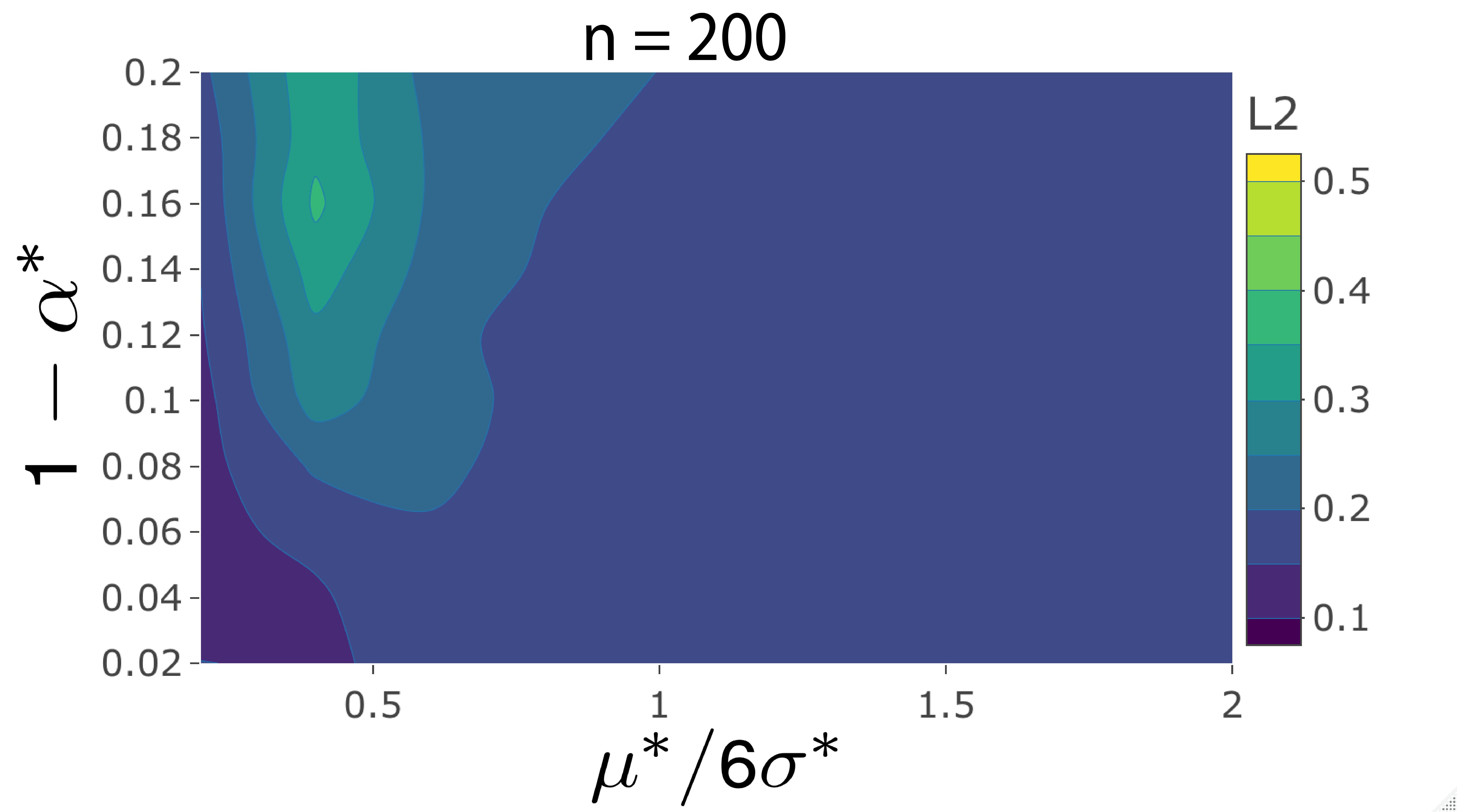
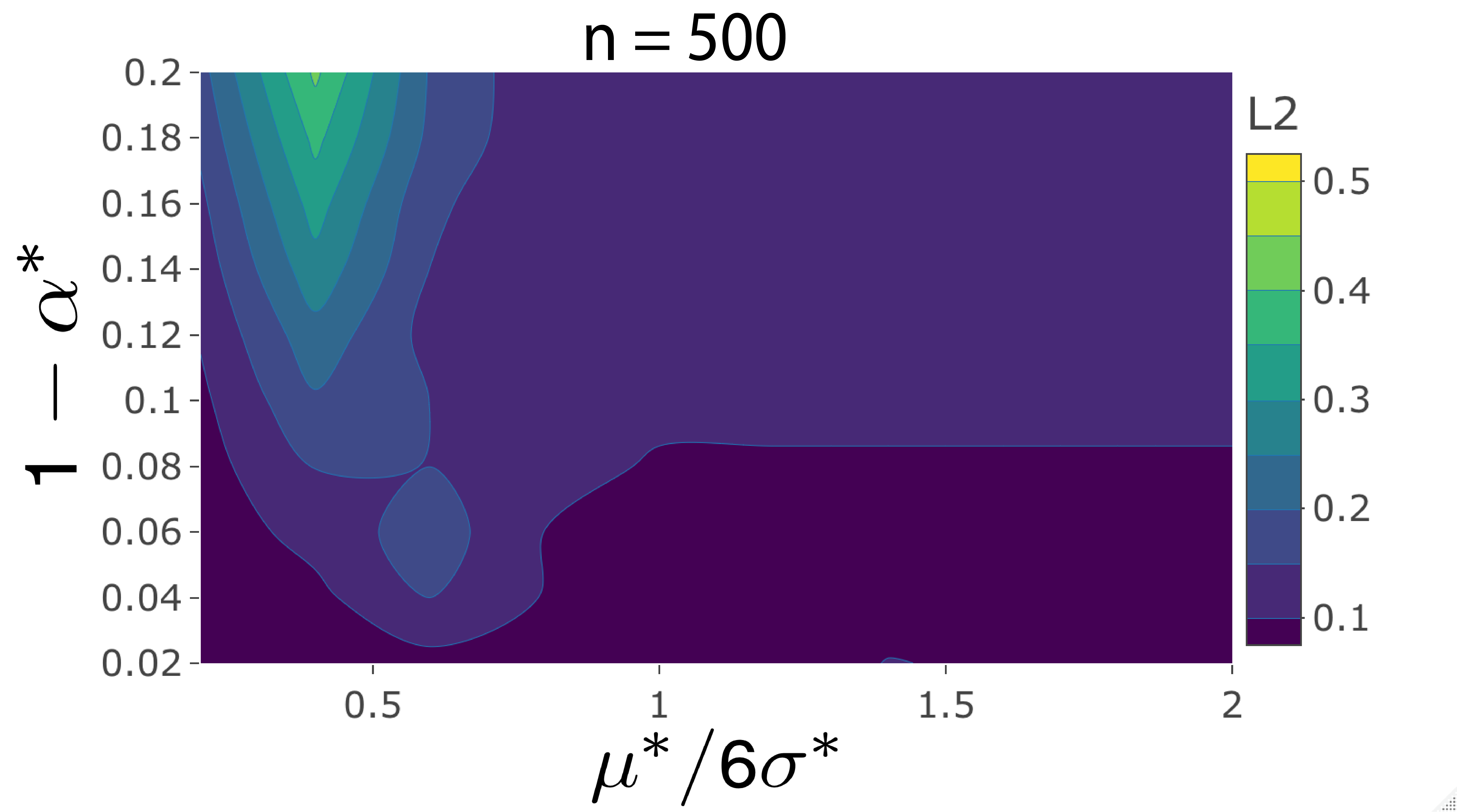
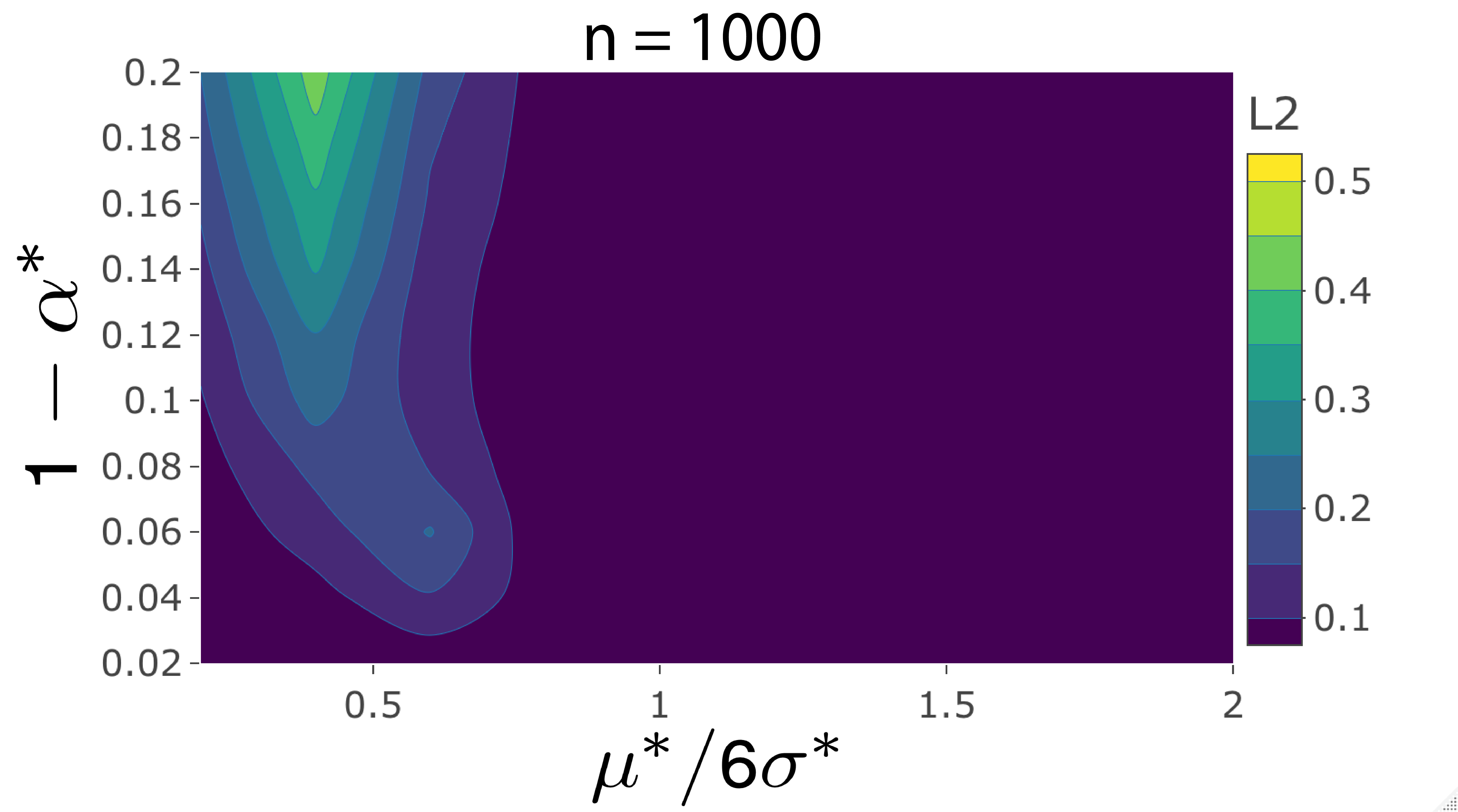
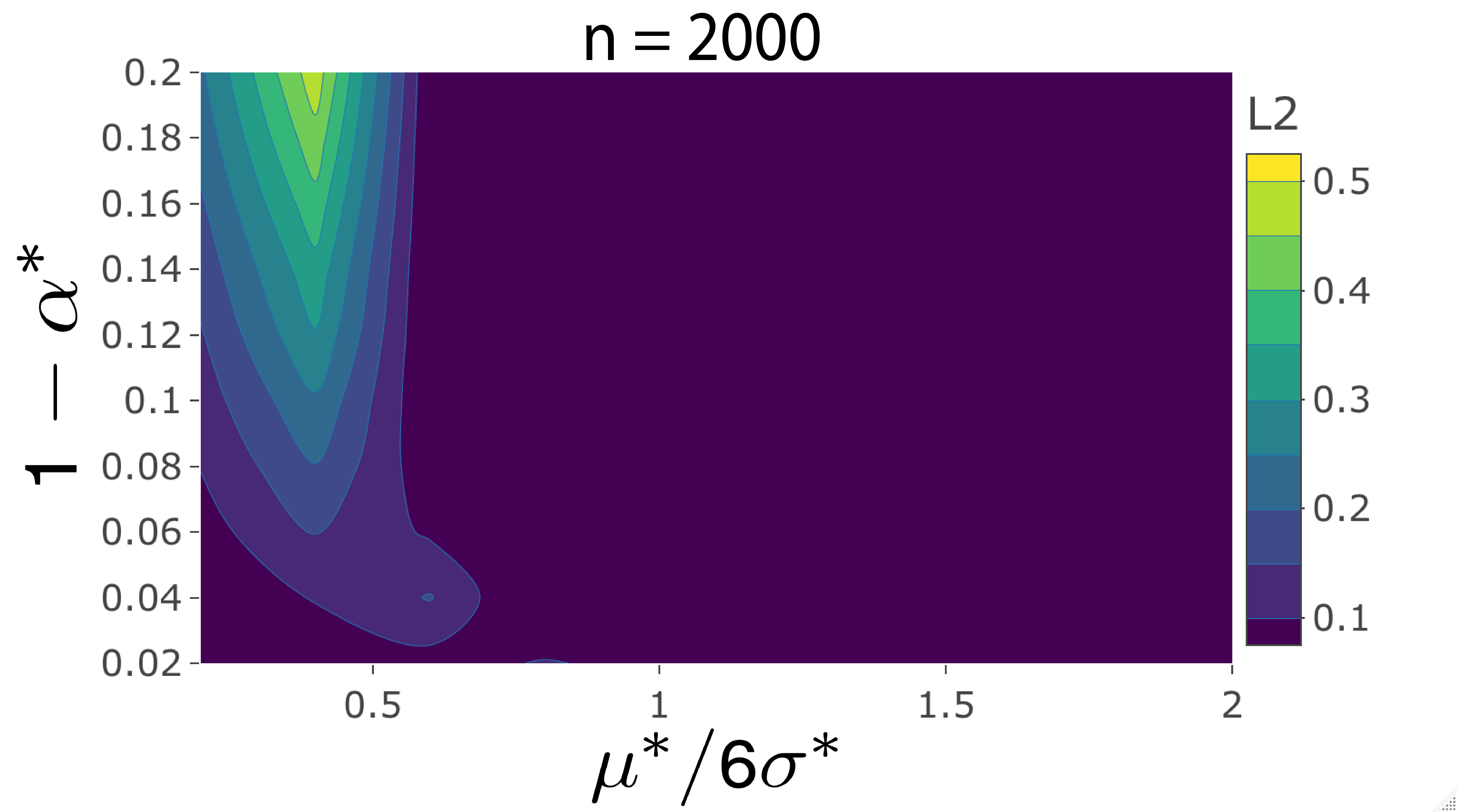
Figure 2: $L_{2}$ error of the smoothEM smooth component estimate on simulated data with uniformly distributed spikes. The contour plots show the error (averaged over $20$ simulation replicates) as a function of the spike percentage ($1-\alpha^{*}$) and the STN $\mu^{*}/(6\sigma^{*})$. From left to right, top to bottom, $n=200,500,1000,2000$.

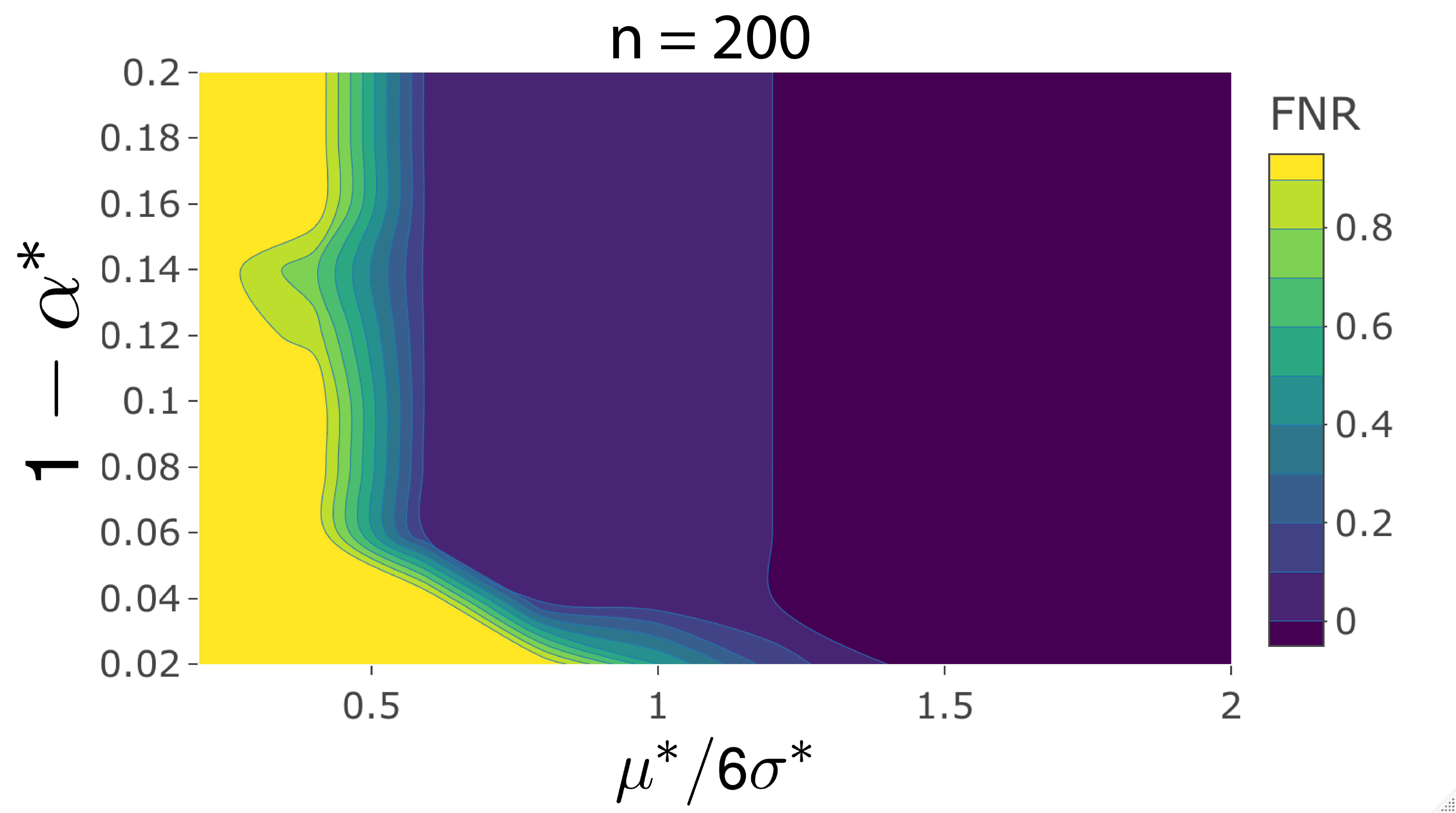
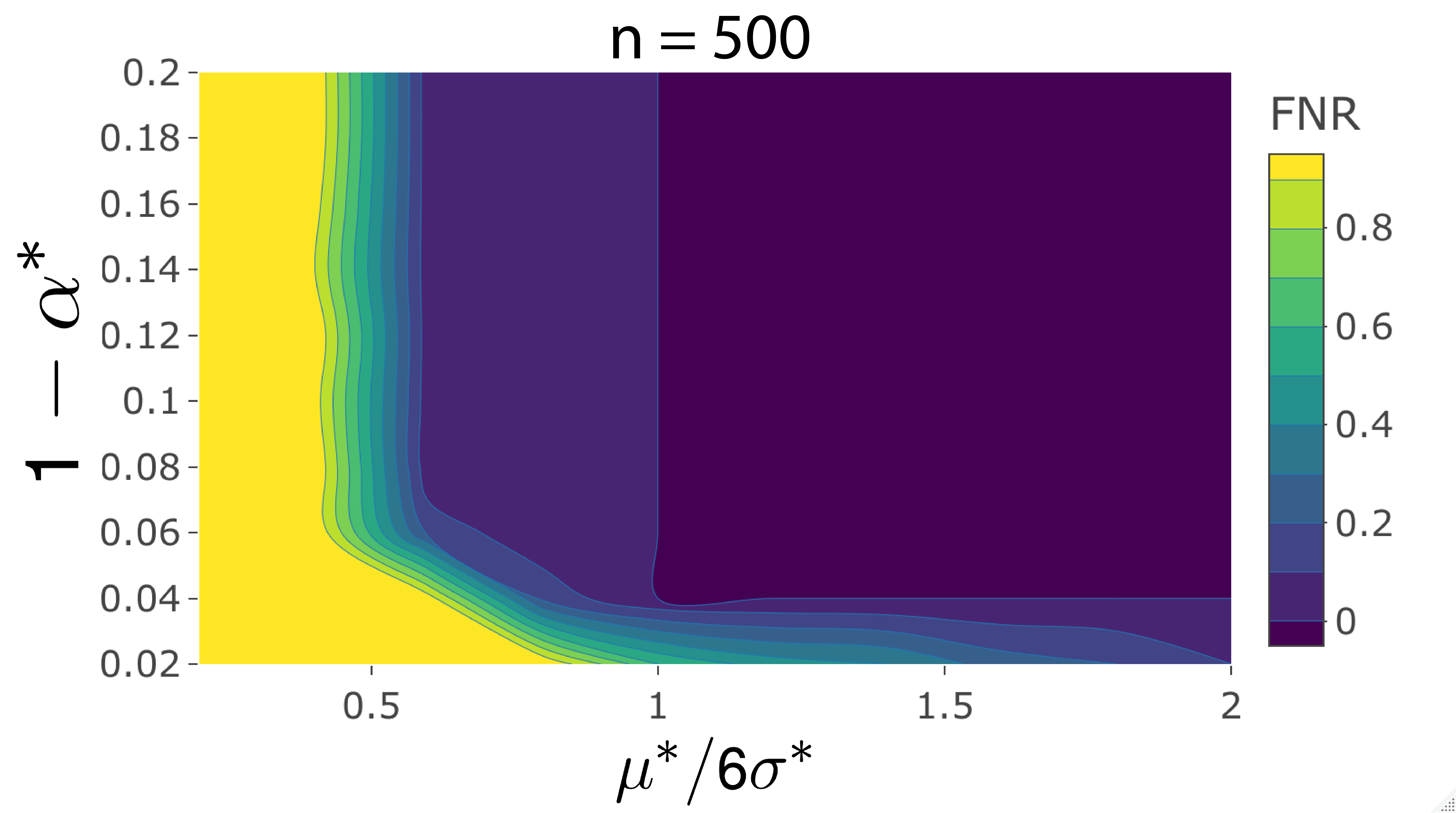
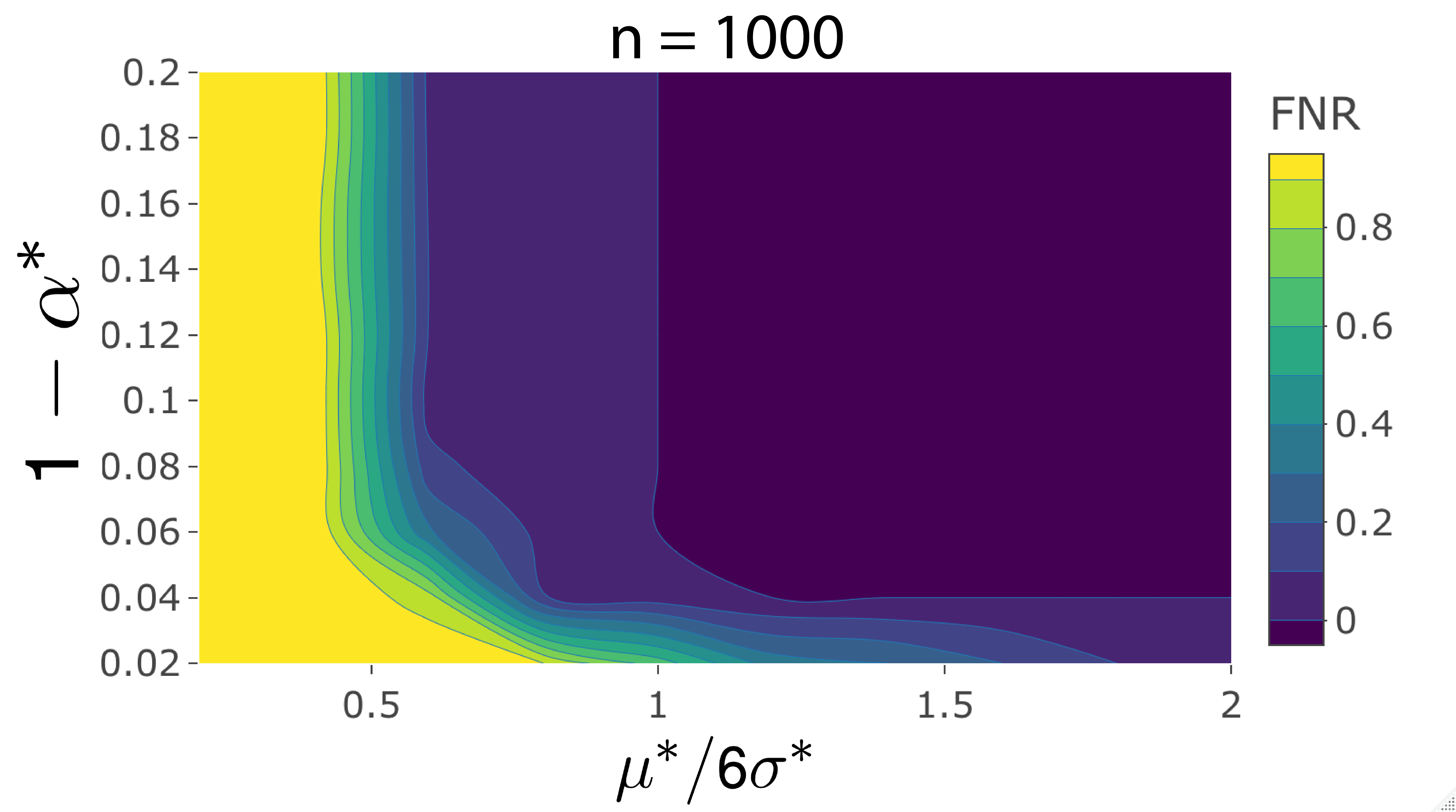
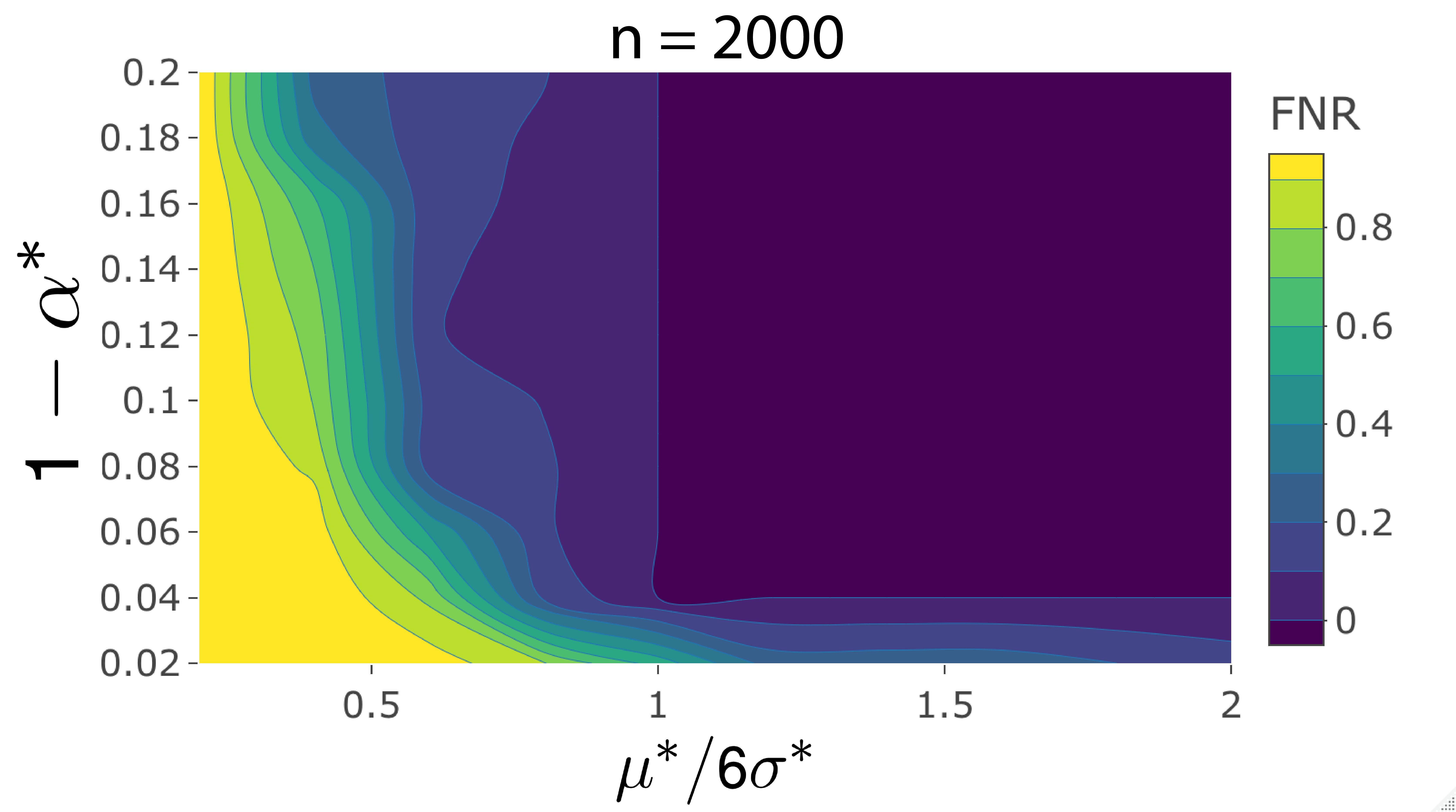
Figure 3: FNR of the smoothEM spike identification on simulated data with uniformly distributed spikes. The contour plots show the FNR (averaged over $20$ simulation replicates) as a function of the spike percentage ($1-\alpha^{*}$) and the STN $\mu^{*}/(6\sigma^{*})$. From left to right, top to bottom, $n=200,500,1000,2000$.

We observe that, when $n$ is large, a sufficiently large signal $\mu^{*}/(6\sigma^{*})\geq 1$ corresponds to low FNR (i.e. good spike classification), and thus low error in estimating the smooth component. When the signal is small, so that spikes are not well separated, our procedure naturally has a harder time recognizing them – but estimation of the smooth component does not suffer much, as smaller spikes do not distort the fit substantially. Notably though, both spike identification and smooth component estimation do improve with larger spike size and lower $\alpha^{*}$, which is in line with our previous discussion in Section 4. Additionally, Figure S2 in the Supplementary Material contains contour plots of the sum of squared error of parameter estimates $\small\|\hat{\theta}-\theta^{*}\small\|_{2}$, with the same format as Figures 2 and 3. Here accuracy is consistent with FNR results, which is to be expected since the mis-classification of spikes affects estimation of $\mu^{*},\sigma^{*}$ and $\alpha^{*}$.

5.2 Non-homogeneous Poisson spikes

The top-right panel in Figure 1 depicts a scenario where spike locations are generated through a non-homogeneous Poisson, as to be “clumped” – instead of uniformly distributed across the domain. To achieve this, our simulation uses a thinning method by Lewis & Shedler (1979). Following their algorithm, the rate function is chosen such that we have spike “clumps” of different sizes. We note that by using a non-homogeneous Poisson distribution, at best, we can only approximate the percentage of contamination. As the locations of spikes are now correlated, the mixture Gaussian model specification will not apply. However, simulation results demonstrate excellent robustness for this type of model mis-specification (see Figures S3-S5 in the Supplementary Material, which are the analogs of the figures in the case of uniformly distributed spikes.) This suggests that soomthEM performs similarly well, and thus that it possesses a degree of robustness to the different ways spikes may be distributed across the domain.

5.3 Comparison to existing methods

Next, we compare smoothEM to a recent baseline correction method called RWSS-GCV (Wei et al., 2022) and a general adaptive smoothing algorithm, implemented via the gam function (with option bs = “ad”) from the mgcv R package Wood (2011) (hereby denoted mgcv-AS). Specifically, we compare $L_{2}$ and $L_{\infty}$ errors in smooth component estimation, i.e. $\small\|\hat{f}(x)-f(x)\small\|_{2}$ and $max_{x}\small[\hat{f}(x)-f(x)\small]$, across methods. We cannot compare spike identification, since RWSS-GCV and mgcv-AS do not identify spikes. We consider both a slow-varying and fast-varying underlying smooth curve a $Beta(4,1)$ density and $9\pi sin(x)$ in $[0,1]$, respectively (see Figure S6 in the Supplementary Material). Each setting is again run $20$ times, and we report average errors.

Table 2 summarizes the performance of the three methods, and shows that smoothEM dominates in most cases. Adaptive smoothing (mgcv-AS), due to its ability to dynamically and locally assign penalty, is more vulnerable to spikes and performs poorly – as it assigns lower penalty to spike-affected area. The only scenario in which mgcv-AS outperforms smoothEM is when both the sample size and the signal-to-noise ratio are low ($n=200$ and $STN=0.4$), making smoothEM more likely to mis-classify spikes and thus deteriorating its smooth curve estimation. Both RWSS-GCV and smoothEM employ iterated penalized smoothing. Whereas RWSS-GCV uses flexible weights to down-weight spikes, smoothEM uses a hard classification scheme (spike/not spike) and performs classification and estimation simultaneously in a probabilistic framework. When the smooth curve is slow-varying, RWSS-GCV trails behind smoothEM by a large margin, probably due to the fact that the latter exploits distributional information about the data. Moreover, RWSS-GCV is highly sensitive to the shape of the smooth curve; its performance worsens dramatically when estimating the fast-varying curve. Lastly, an important observation is that, contrary to smoothEM, both RWSS-GCV and mgcv-AS worsen when the signal-to-noise ratio increase. This suggests that these methods fail to take advantage of the larger separation between spikes and non-spikes to better estimate the smooth curve, and actually include the spikes in this estimation.

Table 2: Comparison of smoothEM, RWSS-GCV and mgcv-AS. Bold entries mark the best performing method in each scenario and for each error.

	$n$	STN	$1-\alpha^{*}$	$L_{2}$			$L_{\infty}$
				mgcv-AS	RWSS-GCV	smoothEM	mgcv-AS	RWSS-GCV	smoothEM
		2	0.1	3.4014	1.4756	0.0298	4.8207	2.1527	0.4213
		2	0.05	0.7572	1.1956	0.0308	2.4117	1.9272	0.4297
		1	0.1	0.8475	0.8234	0.0298	2.3363	1.8039	0.4213
		1	0.05	0.1905	0.9652	0.0308	1.0712	1.7230	0.4298
		0.4	0.1	0.1352	0.3609	0.1581	0.7771	1.1084	0.7222
	200	0.4	0.05	0.0453	0.1051	0.2479	0.4692	0.6166	0.8674
		2	0.1	2.6524	0.7562	0.0095	3.8448	1.9553	0.2243
		2	0.05	0.5592	0.4329	0.0057	2.1240	1.3041	0.2008
		1	0.1	0.7143	0.3901	0.0100	2.0590	1.2149	0.2259
		1	0.05	0.1698	0.4157	0.0060	1.1372	1.2619	0.2016
		0.4	0.1	0.1437	0.1678	0.1249	0.9306	0.7322	0.6172
S L O W - V A R Y I N G	500	0.4	0.05	0.0519	0.3509	0.0419	0.4914	0.9738	0.3830
		2	0.1	3.4899	8.4221	0.0456	4.8757	4.4467	0.6868
		2	0.05	0.8817	7.1128	0.0458	2.8577	4.0532	0.7235
		1	0.1	0.8803	4.8541	0.1064	2.3539	3.4204	0.8284
		1	0.05	0.2304	3.9899	0.0483	1.3602	2.8410	0.7250
		0.4	0.1	0.1352	0.3609	0.1581	0.7771	1.1084	0.7222
	200	0.4	0.05	0.0453	0.1051	0.2479	0.4692	0.6166	0.8674
		2	0.1	2.6753	3.6666	0.0225	3.9582	2.8876	0.6094
		2	0.05	0.5986	4.5329	0.0181	2.2317	2.9951	0.6014
		1	0.1	0.7228	3.7041	0.0331	2.0649	2.6321	0.5704
		1	0.05	0.1818	4.5263	0.0273	1.1663	3.0404	0.5952
		0.4	0.1	0.1493	3.3939	0.2239	0.9525	2.2901	1.1147
F A S T - V A R Y I N G	500	0.4	0.05	0.0569	2.3397	0.0696	0.5834	2.1700	0.6490

6 Data applications

6.1 Smart meter electricity data

We consider data from the Smart Meter Electricity project of the Irish Commission for Energy Regulation, which collected data on electricity consumption from over 5000 households and businesses during 2009 and 2010. Our goal here is to create a meaningful statistical representation of the electricity consumption behaviors, which may be useful to policy makers.

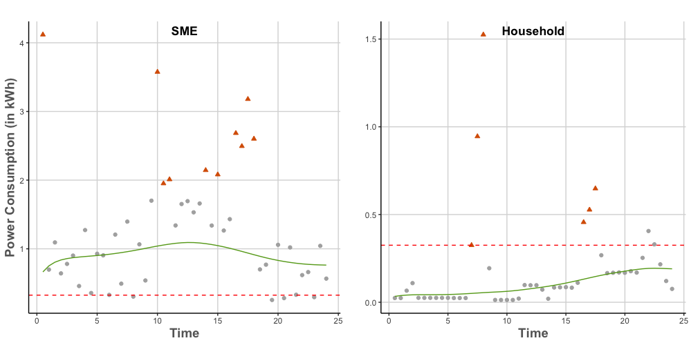
Figure 4: Electricity consumption by an Irish small business (left) and an Irish household (right) on Jan 5, 2010. The estimated smooth components are plotted in green, whereas spikes are identified by red triangles. The red horizontal dashed lines placed at 0.3 on the vertical axes help visualize the different magnitudes of consumption.

We assume that consumption predominantly follows a smooth pattern with occasional spiked activity – e.g. when multiple electrical devices are turned on simultaneously. The data contains daily measurements of electricity consumed, collected at 30 minute intervals in kWh, for each household and business in the study. As an illustration, we run our procedure on data from one household (meter ID 1976) and one small business enterprise (SME, meter ID 1977) for the months of January and July in 2010. This allows us to highlight differences in patterns of power usage between households and business, and winter and summer months. A visual inspection of two exemplar time series, shown in Figure 4, suggests that assuming the error variances at smooth and spike locations to be the same, as we do in Equation (2), may be too restrictive here. Therefore, we allow errors to have inflated variance at spike locations; that is, we use the model described by Equation (3). This adds a new variance parameter to be estimated in the EM algorithm, which is not covered in our theoretical treatment in Section 4.2, but does not cause any convergence slow-down in this application. We also adopt the grid $(10^{4},\ldots,10^{-4})$ for the tuning parameter $\lambda$.

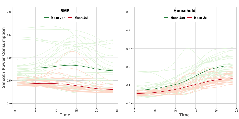
Figure 5: Electricity consumption by an Irish small business (left) and an Irish household (right) for the months of January and July, 2010. Estimated smooth components for each day in January and July are plotted in light green and light red, respectively. The corresponding monthly means are plotted in darker green/red.

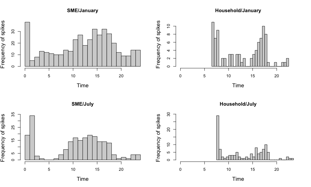
Figure 6: Frequencies of estimated spikes in electricity consumption by an Irish small business (left) and an Irish household (right), for each hour of the day during January, 2010 (top) and July, 2010 (bottom).

Figure 5 shows estimated smooth curves for the household and small business considered across all January and July days. We clearly see that, for both entities, power consumption is higher in January (likely due to heating during cold weather) but follows the same daily pattern in January and July. We also clearly see that such daily pattern is rather different for the small business and the household. Power usage tends to peak during the day for the former and at night for the latter. Notably, power usage by the small business is also more variable (from one day to another) than that by the household – which appears much more consistent. Figure 6 shows monthly frequencies of estimated spikes in every hour of the day, plotted again for the household and small business considered and for January and July. Notably, the household spikes predominantly occur in the early morning (7:00-8:00am) and, in January, in mid-afternoon (4:00-5:00pm). The small business has numerous spikes in the period of the day when its smooth consumption component is highest (approximately 10:00am to 5:00pm) and, interestingly, right after midnight – this may correspond to the automatic activation of some appliances.

6.2 Extreme temperatures in United States

We consider two temperature-related time series in the US, covering the period from 1910 to 2015. The first is the series of the annual heatwave index. This index treats as a heatwave any period of four or more days with an unusually high average temperature (i.e. an average temperature that is expected to occur once every 10 years), and takes on values as a function of geographical spread and frequency of heatwaves. The second is the series of the annual percentage of US land area with unusually high summer temperatures. A visual inspection of the two time series again suggests that the error variances at spike locations are inflated. This can be appreciated in Figure 7. We thus use again the variance inflated model as in the first application. Using the grid $(10^{4},\ldots,10^{-4})$ for the tuning parameter $\lambda$, our procedure yields the spike identification and estimated smooth curves shown in red triangles and green lines, respectively, in Figure 7.

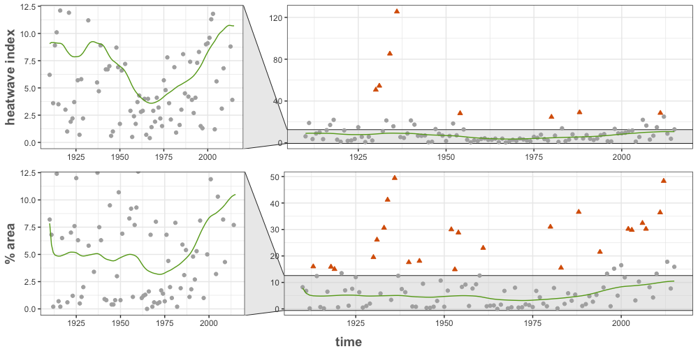
Figure 7: Annual heatwave index in the US (top) and share of its land with unusually high summer temperature (bottom). The estimated smooth component is plotted in green, whereas spikes are identified by the red triangles. For each plot, a vertical zoom (on the left) allows us to visualize the upward trend in the smooth components of both signals in recent decades.

Probably because geographical spread is part of the definition of the heatwave index, the two time series show rather similar underlying trends. smoothEM detects the 1936 North American heat wave, one of the most intense in modern history, both in terms of heat index and of US area affected by high temperatures – along with a number of other spikes. Interestingly, only one spike detected in the heatwave index series concerns recent decades – likely due to the fact that the smooth component estimate exhibits an upward trend; what classified as a spike in the 50’s, or even the 80’s, is consistent with a standard oscillation around a growing systematic value in more recent times. The picture is different for the US area time series; here recent decades exhibit both an increasing smooth component estimate and an abundance of detected spikes – suggesting that the geographical dimension of the problem may be yet more concerning. The estimated values for $\alpha^{*},\mu^{*},\sigma^{*2}_{\epsilon},\sigma^{*2}_{h}$ are respectively $0.08,30.83,5.77,30.79$ for the heatwave index, and $0.28$, $17.88$, $3.96,10.49$ for the US area.

7 Discussion

In this article we propose smoothEM – a procedure that, given a signal, simultaneously performs estimation of its smooth component and identification of spikes that may be interspersed within it. smoothEM uses regularized spline smoothing techniques and the EM algorithm, and is suited for the many applications in which the data comprises discontinuous irregularities superimposed to a noisy curve. We lay out conditions for the procedure to work, and prove asymptotic convergence properties of the EM to a neighborhood of the global optimum under certain restricted conditions. We also demonstrate the effectiveness of smoothEM under departures from such restricted conditions through simulations and two real data applications, and compare it with a recent algorithm that addresses a similar setting (Wei et al., 2022), as well as with adaptive smoothing (mgcv package in R), which penalizes dynamically spike-affected regions. We demonstrate the superiority of smoothEM in a broad range of scenarios. Notably, since it separates spikes and smooth component, smoothEM could also be used to pre-process functional data prior to the use of other FDA tools. For instance, in a regression context, instead of introducing a functional predictor obtained though traditional spline smoothing of the row data, one could apply our procedure and introduce two distinct predictors; namely, the estimated $\hat{f}$ and, separately, the flagged spike locations. As another example, when performing functional motif discovery or local clustering (Cremona & Chiaromonte, 2022), smoothEM could produce “de-spiked” versions of the curves to be searched for recurring smooth patterns, and patterns of detected spikes could be analyzed separately. We shall leave these and other possibilities for future work. An R implementation of smoothEM and some examples are provided at https://github.com/hqd1/smoothEM

Supplementary Material

The Supplementary Material includes technical proofs and additional figures.

References

- (1)
- Balakrishnan et al. (2017) Balakrishnan, S., Wainwright, M. J. & Yu, B. (2017), ‘Statistical guarantees for the EM algorithm: from population to sample-based analysis’, The Annals of Statistics 45(1), 77–120.
- Cremona & Chiaromonte (2022) Cremona, M. A. & Chiaromonte, F. (2022), ‘Probabilistic k-means with local alignment for clustering and motif discovery in functional data’, Journal of Computational and Graphical Statistics 0(ja), 1–17.
- de Boor (1978) de Boor, C. (1978), A practical guide to splines, Springer.
- Descary & Panaretos (2019) Descary, M. H. & Panaretos, V. M. (2019), ‘Functional data analysis by matrix completion’, The Annals of Statistics 47(1), 1–38.
- Goldsmith et al. (2011) Goldsmith, J., Bobb, J., Crainiceanu, C. M., Caffo, B. & Reich, D. (2011), ‘Penalized functional regression’, Journal of Computational and Graphical Statistics 20(4), 830–851.
- Kokoszka & Reimherr (2017) Kokoszka, P. & Reimherr, M. (2017), Introduction to Functional Data Analysis, CRC Press.
- Lewis & Shedler (1979) Lewis, P. A. W. & Shedler, G. S. (1979), ‘Simulation of Nonhomogeneous Poisson Processes with Degree-Two Exponential Polynomial Rate Function’, Operations Research 27(5), 1026–1040.
- Luo & Wahba (1997) Luo, Z. & Wahba, G. (1997), ‘Hybrid Adaptive Splines’, Journal of the American Statistical Association 92, 107–116.
- Nason (2008) Nason, G. P. (2008), Wavelet Methods in Statistics with R, Springer.
- O’Sullivan (1986) O’Sullivan, F. (1986), ‘A statistical perspective on ill-posed inverse problems’, Statistical Science 1(4), 502–518.
- Pintore et al. (2006) Pintore, A., Speckman, P. & Holmes, C. C. (2006), ‘Spatially adaptive smoothing splines’, Biometrika 93(1), 113–125.
- Ramsay & Silverman (2007) Ramsay, J. O. & Silverman, B. (2007), Applied functional data analysis: methods and case studies, Springer.
- Wei et al. (2022) Wei, J., Zhu, C., Zhang, Z. M. & He, P. (2022), ‘Two-stage iteratively reweighted smoothing splines for baseline correction’, Chemometrics and Intelligent Laboratory Systems 227, 104606.
- Wood (2011) Wood, S. N. (2011), ‘Fast stable restricted maximum likelihood and marginal likelihood estimation of semiparametric generalized linear models’.
- Wu et al. (2017) Wu, C., Yang, C., Zhao, H. & Zhu, J. (2017), On the convergence of the em algorithm: A data-adaptive analysis. arXiv:1611.00519v2.
- Xiao (2019) Xiao, L. (2019), ‘Asymptotic theory of penalized splines’, Electronic Journal of Statistics 13, 747–794.
- Yao & Lee (2006) Yao, F. & Lee, T. C. M. (2006), ‘Penalized spline models for functional principal component analysis’, Journal of the Royal Statistical Society: Series B (Statistical Methodology) 68(1), 3–25.
- Zhang et al. (2010) Zhang, Z. M., Chen, S. & Liang, Y. Z. (2010), ‘Baseline correction using adaptive iteratively reweighted penalized least squares’, Analyst 135(5), 1138–1146.