PAC-Net: A Model Pruning Approach to Inductive Transfer Learning

Abstract

Inductive transfer learning aims to learn from a small amount of training data for the target task by utilizing a pre-trained model from the source task. Most strategies that involve large-scale deep learning models adopt initialization with the pre-trained model and fine-tuning for the target task. However, when using over-parameterized models, we can often prune the model without sacrificing the accuracy of the source task. This motivates us to adopt model pruning for transfer learning with deep learning models. In this paper, we propose PAC-Net, a simple yet effective approach for transfer learning based on pruning. PAC-Net consists of three steps: Prune, Allocate, and Calibrate (PAC). The main idea behind these steps is to identify essential weights for the source task, fine-tune on the source task by updating the essential weights, and then calibrate on the target task by updating the remaining redundant weights. Under the various and extensive set of inductive transfer learning experiments, we show that our method achieves state-of-the-art performance by a large margin.

1 Introduction

Deep neural networks trained with massive data have exceeded humans in accuracy across various tasks, e.g., vision recognition (He et al., 2016) or natural language processing (Rajpurkar et al., 2016). However, in real-world situations where the training samples are scarce, the performance of deep neural networks often deteriorates significantly. Transfer learning techniques have been introduced to overcome such performance degradation in the small data regime (Pan & Yang, 2009). In particular, inductive transfer learning is a promising framework that allows learning with a limited target dataset by leveraging a pre-trained source model, under the assumption that the source and target tasks are closely related to each other (Li et al., 2018) (Li et al., 2019). For successful inductive transfer learning with deep neural networks, it is crucial to utilize the weights of the source model by transferring the core knowledge embedded in the weights to the target model. Typically, it is realized by fine-tuning (Yosinski et al., 2014) which initializes the weight vector of the target model as that pre-trained on the source task. Some follow-up studies (Li et al., 2018; Li & Zhang, 2021; Li et al., 2019) further regularize the target model to prevent diverging from the source weight vector during the fine-tuning.

However, we found that these methods can easily overfit the target data despite their novel initialization and regularization. We hypothesize that this is because the model cannot preserve the core source knowledge when learning the target data. Consider a simple problem of learning dynamics for a real-world oscillator (e.g., a spring-mass-damper system), as depicted in Figure 1. The conservation of energy is one of the principal laws that govern the dynamical behavior of the ideal spring-mass system (top of Figure 1 (a)). On the other hand, the real-world oscillator interacts with the environment, thus losing its mechanical energy due to the damping factor (bottom of Figure 1 (a)). What we expect from inductive transfer learning is that the model learns the law of the conservation of energy from the source task, then recognizes the damping term that causes the energy loss from a small number of measured target samples. The leftmost column of Figure 1 (b) shows the model pre-trained on the source data has learned the energy conservation principle. After the fine-tuning process (Yosinski et al., 2014; Li et al., 2018, 2019), unfortunately, the model overfits on few samples and forgets the law of conservation of energy; as shown in the center of Figure 1 (b), the transferred model predicts the oscillator gains its energy from the environment, which violates the fundamental law of physics.

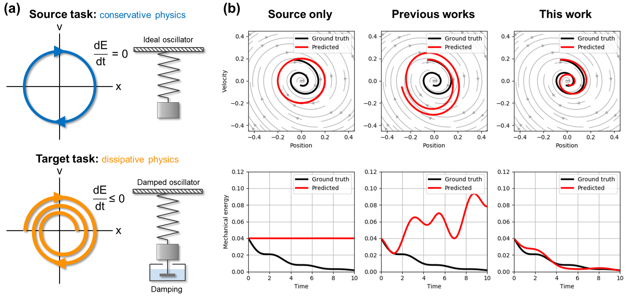
Figure 1: (a) Description of the source and target tasks. (b) Phase and energy-versus-time plot. What (a) and the leftmost of (b) illustrate is that the source and target systems are conservative and dissipative, respectively. What stands out in the rightmost of (b) is that our work can predict real physics by keeping the source knowledge (conservation of energy) and learning the target data (loss of energy) while the center (previous works) of (b) cannot.

To overcome this problem, we propose a simple yet effective algorithm that can learn the target task (e.g., loss of energy) while preserving the relevant knowledge obtained from the source task (e.g., conservation of energy), as shown in the rightmost of Figure 1 (b). This is achieved by decomposing the weights into two disjoint sets, where one is in charge of learning the source task and the other for the target task, by adopting the pruning technique. More specifically, the algorithm consists of the following three steps: pruning, allocation, and calibration (PAC), which we call PAC-Net. In the pruning step, we sparsify the deep neural network pre-trained on the source task dataset. Then, we allocate the unpruned ($\mathbf{w}_{U}$) and pruned weights ($\mathbf{w}_{P}$) to transferable and calibratable parts, respectively. Finally, we calibrate $\mathbf{w}_{P}$ with the target task samples. The contribution of our work is summarized below:

• Our method provides a unified transfer learning approach for classification and regression as well as non-convolutional neural networks, which is of more general applicability compared to previous work.

• To our best knowledge, our paper is the first study to provide transfer learning experiments on solving ODEs and PDEs, an impactful task for machine learning to solve scientific problems.

• Our method for preserving source knowledge through pruning with regularization makes the model mitigate catastrophic forgetting, which achieves state-of-the-art performance.

This paper is organized as follows. Section 2 reviews the previous works related to our work. Section 3 describes PAC-Net in detail. Section 4 shows experimental results of the proposed method on various domains. Section 5 concludes this paper with a brief remark.

2 Related Works

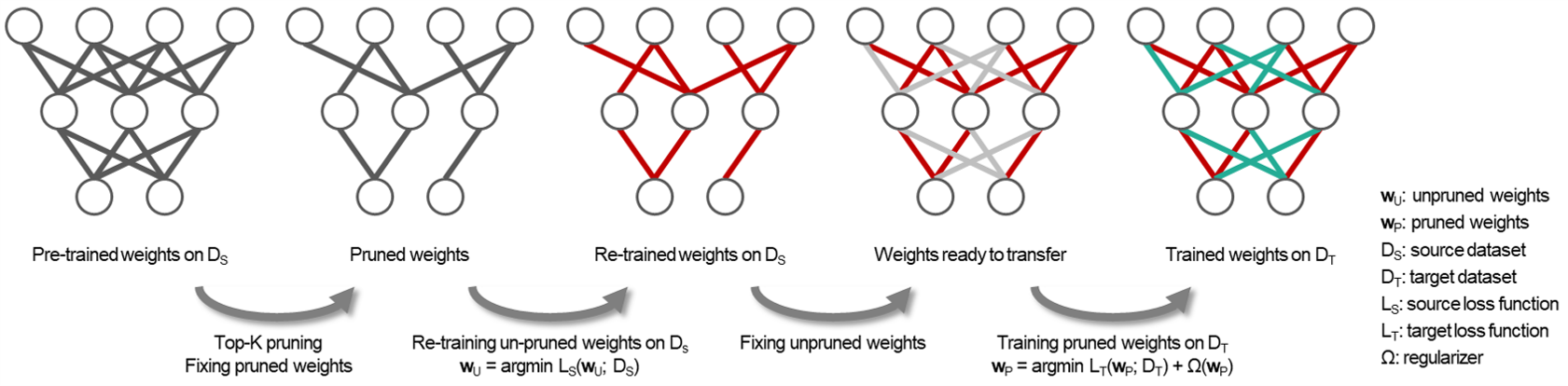
Figure 2: PAC-Net operates in three steps. In the first step, PAC-Net prunes inconspicuous weights after initially training the network with source data. In the second step, PAC-Net allocates the unpruned and pruned weights for the source and the target task, respectively. in this step, PAC-Net re-trains the source task with unpruned weights and keeps the pruned weights to zero. At last, PAC-Net calibrates the pruned weights with few target samples while regularizing them to be not too far from zero.

2.1 Transfer Learning

Following the nomenclature in (Pan & Yang, 2009), transfer learning can be categorized into transductive transfer learning (i.e. domain adaptation) and inductive transfer learning. We briefly review some of the previous work on domain adaptation and inductive transfer learning.

Domain adaptation.

Transductive transfer learning is usually called domain adaptation, where tasks are the same and the domains are different but related to each other. The domain adaptation is categorized into supervised (with a few labels in the target domain) and unsupervised (without labels in the target domain) settings. In supervised domain adaptation, classification and contrast semantic alignment (CCSA) (Motiian et al., 2017) and domain adaptation using stochastic neighborhood embedding (Xu et al., 2019) use two stream architectures and introduce loss functions to reduce the distances among intra-class data pairs in the embedding space while maximizing the distances among inter-class data pairs. In unsupervised domain adaptation, many approaches attempt to align statistical distribution shift between the source and target domains (Sun & Saenko, 2016; Yan et al., 2017; Zellinger et al., 2017), or employ discriminators for domain alignment (Tzeng et al., 2017; Ajakan et al., 2014).

Inductive transfer learning.

On the other hand, inductive transfer learning, which is the focus of this paper, refers to the case where tasks are different but related to each other, while domains are the same. Typically, the relationship between learning simulation models (the source) and real-world physical phenomena (the target) can be explained by inductive transfer learning task. It is crucial how to utilize the weights of the source task when training on the target task. Here, let us briefly review the literature.

Boosting ensemble employs additional networks to correct errors made by networks learning the source task. AdaBoost (Freund & Schapire, 1997) is an adaptive method in which subsequent weak learners train instances that are misclassified by previous classifiers. (Yao & Doretto, 2010) and (Pardoe & Stone, 2010) extended AdaBoost to transfer learning for classification and regression. These approaches, however, incur high computational costs when employing a large network as the base learner.

Another approach utilizes the weights of the source model as initial weights to train the target task, known as fine-tuning. (Yosinski et al., 2014) has demonstrated the representation, learned from the source task, can be transferred to the target tasks. (Li et al., 2018) compares a number of different regularization strategies that make the weights of the source model and the target model similar during fine-tuning. (Li et al., 2019) preserves a subset of feature maps from the source model with channel-wise attention to align activations from the CNN layers of source and target models.

2.2 Network Pruning

Extending the classical work on Optimal Brain Damage (LeCun et al., 1990) and Optimal Brain Surgeon (Hassibi et al., 1993), Han et al. (2015) suggested an iterative training pipeline for model efficiency that alternates between network pruning and fine-tuning. In their follow-up work, (Han et al., 2017) increased the model capacity by removing the sparsity constraint, re-initialized the pruned parameters to zero, and finally re-trained the whole dense network. PackNet (Mallya & Lazebnik, 2018), designed for continual learning (lifelong learning), also employed the pruned parameters to add the new task in the same domain while avoiding catastrophic forgetting (McCloskey & Cohen, 1989). In improving the pruned sparse network for higher accuracy, (Frankle & Carbin, 2019) strongly emphasized the importance of the initial weights determined in the network before pruning. On the other hand, our method is different from the above methods. To reduce the gap between source and target task performances, we suggest the pruned weights should be set to zero and fit the target data with the pruned weights, with regularization to prevent the weight updates deviating too far from zero.

3 Proposed Method

Formal definition of inductive transfer learning.

Let $\mathcal{X}$ and $\mathcal{Y}$ be the input and output spaces, respectively. We will consider two related but different datasets defined on $\mathcal{X}\times\mathcal{Y}$. The first is the source dataset $\mathcal{D}_{S}=\{(x_{S}^{i},y_{S}^{i})\}_{i=1}^{N_{S}}$, where $(x_{S}^{i},y_{S}^{i})\sim p_{S}(x_{S},y_{S})=p_{S}(y_{S}|x_{S})p(x_{S})$. Similarly, the second is the target dataset ${D}_{T}=\{(x_{T}^{i},y_{T}^{i})\}_{i=1}^{N_{T}}$ realized from $p_{T}(x_{T},y_{T})=p_{T}(y_{T}|x_{T})p(x_{T})$. It should be noted that both datasets share the same input distribution $p(\cdot)$. On the other hand, the conditional distribution $p_{S}(\cdot|x)$ and $p_{T}(\cdot|x)$ are assumed to be different, yet related. The number of target samples is much smaller than that of source samples, i.e., $0\leq N_{T}\ll N_{S}$. The (supervised) inductive transfer learning is defined as learning $p_{T}(\cdot|x)$ (or equivalently the model $f_{T}:\mathcal{X}\to\mathcal{Y}$), by exploiting the knowledge obtained from the source task. For neural network models, it is generally realized by transferring the weights of the source model to the target one, e.g., based on the fine-tuning.

Fine-tuning.

Let $f_{\mathbf{w}_{S}}:\mathcal{X}\to\mathcal{Y}$ be a pre-trained model on the source dataset $\mathcal{D}_{S}$ where $\mathbf{w}_{S}\in\mathbb{R}^{D}$ denotes $D$-dimensional weight vector of the pre-trained model. Given the target dataset $\mathcal{D}_{T}$, the fine-tuning method minimizes the standard negative log-likelihood (NLL) $\mathcal{L}_{T}(\mathbf{w})=-\sum_{i=1}^{N_{T}}\log p_{\mathbf{w}}(y_{T}^{i}|x_{T}^{i})$ using the stochastic gradient descent:

$$\mathbf{w}(t+1)=\mathbf{w}(t)-\eta\hat{\nabla}_{\mathbf{w}}\mathcal{L}_{T}(\mathbf{w}),\;\mathbf{w}(0)=\mathbf{w}_{S},$$ (1)

where $\eta$ is a step size and $\hat{\nabla}_{\mathbf{w}}\mathcal{L}_{T}(\mathbf{w})$ denotes a stochastic estimate of the loss gradient using a mini-batch of data. Thus, the fine-tuning is a maximum likelihood estimation whose the log-prior is centered at $\mathbf{w}_{S}$.

Starting point (SP) regularization.

Much of the previous work argued that the above simple fine-tuning can lead to a catastrophic forgetting of the source knowledge relevant to the targeted task (Li et al., 2018; Chen et al., 2019; Li et al., 2019, 2020; Chen et al., 2020). It is because some important weights may be driven far away from their initial $\mathbf{w}_{S}$. To overcome this issue, (Li et al., 2018) proposed starting point (SP) regularization that explicitly encourages the transferred target weight to be close to the initial source weight. Specifically, $L^{2}$-SP regularization is given by:

$$\Omega(\mathbf{w})=\lambda\|\mathbf{w}-\mathbf{w}_{S}\|^{2}=\lambda\sum_{i=1}^{D}|w^{i}-w_{S}^{i}|^{2},$$

where $\lambda$ is a regularization parameter. With the $L^{2}$-SP regularizer, the fine-tuning process (1) is modified as a maximum a posterior estimation with the log-prior of $\mathbf{w}_{S}$:

$$\mathbf{w}(t+1)=\mathbf{w}(t)-\eta\hat{\nabla}_{\mathbf{w}}[\mathcal{L}_{T}(\mathbf{w})+\Omega(\mathbf{w})],\;\mathbf{w}(0)=\mathbf{w}_{S}.$$ (2)

The advantage of SP regularization over the standard fine-tuning is theoretically proved as well as empirically validated (Li et al., 2018; Gouk et al., 2020; Li & Zhang, 2021). However, we found that (2) is still ineffective for transferring the core source knowledge, especially when the amount of the target samples is limited (see experimental results in Section 4). This is the main motivation behind our work, hypothesizing that keeping the relevant weights unchanged is more crucial than constraining all the weights softly.

All you need is pruning.

Let $\mathbf{w}_{U}\in\mathbb{R}^{K}$ and $\mathbf{w}_{P}\in\mathbb{R}^{D-K}$ be the top-$K$ relevant weights and the remainder, respectively, i.e., $\mathbf{w}(t)=\mathbf{w}_{U}\oplus\mathbf{w}_{P}(t)$. We propose a modified transfer learning scenario of (2) that only updates $\mathbf{w}_{P}(t)$ while $\mathbf{w}_{U}$ fixed at SP:

$$\begin{split}&\mathbf{w}_{P}(t+1)=\mathbf{w}_{P}(t)-\eta\hat{\nabla}_{\mathbf{w}_{P}}[\mathcal{L}_{T}(\mathbf{w})+\Omega(\mathbf{w}_{P})],\\ &\mathbf{w}(0)=\mathbf{w}_{U}+\mathbf{w}_{P}(0),\;\Omega(\mathbf{w}_{P})=\lambda\sum_{i=1}^{D-K}|w_{P}^{i}-w_{p}^{i}(0)|^{2}.\end{split}$$ (3)

Note that the choice of $\mathbf{w}_{U}$ is highly important for (3). An ideal situation would be that the weight space is decomposed with respect to the source knowledge, i.e., all of the source information should be embedded in $\mathbf{w}_{U}$ before the transfer learning. In other words, $f_{\mathbf{w}_{U}}$ should be the equivalent sub-network of $f_{\mathbf{w}_{S}}$. Meanwhile, the remainder $\mathbf{w}_{P}$ should have enough capacity to learn the target task.

Fortunately, the Lottery Ticket Hypothesis (LTH) states that there is an equivalent ($\mathcal{L}_{S}(\mathbf{w}_{U})\leq\mathcal{L}_{S}(\mathbf{w}_{S})$ where $\mathcal{L}_{S}$ is NLL for the source task) yet efficient ($K\ll D$) sub-network representation of the source model (Frankle & Carbin, 2019). In addition, there are a number of notable works that theoretically guarantee LTH or suggest pruning techniques to find such a sub-network practically (Malach et al., 2020; Lubana & Dick, 2020; Zhang et al., 2021).

PAC-Net.

Inspired by the above, we propose PAC-Net: firstly Prune the source model, secondly Allocate the unpruned ($\mathbf{w}_{U}$) and pruned weights ($\mathbf{w}_{P}$) for fixed and learnable parts with respect to the target task, and finally Calibrate $\mathbf{w}_{P}$ via (3) with few target data. In the following paragraphs, we explain how PAC-Net operates for each step in detail.

Step 1: Pruning.

In this paper, we use the magnitude-based pruning as a baseline method (Han et al., 2015; Lubana & Dick, 2020). It prunes the weight vector $\mathbf{w}_{S}=(w_{S}^{1},...,w_{S}^{D})^{T}$ of the pre-trained model $f_{\mathbf{w}_{S}}$ by applying the following binary mask $\mathbf{m}=(m^{1},...,m^{D})^{T}$ that keeps the top-$K$ large-magnitude weights:

$$m^{i}=\begin{cases}1,&\text{if }|w^{i}|>w_{\kappa}\\ 0,&\text{otherwise,}\end{cases}$$

where $w_{\kappa}$ is a threshold value determined by $K$. We summarize the pruning step in Algorithm 1.

Input: pre-trained weight $\mathbf{w}$

$w_{\kappa}=\texttt{sort}(|\mathbf{w}|)_{K}$;

$\mathbf{m}=\mathbbm{1}(|\mathbf{w}|-w_{\kappa})$;

Output: pruning mask $\mathbf{m}$;

Algorithm 1 Pruning

Step 2: Allocation.

Because all the information on the source task should be embedded in the unpruned weights $\mathbf{w}_{U}=\mathbf{w}\odot\mathbf{m}$, we re-train the masked neural network with fixing:

$$\begin{split}\mathbf{w}_{U}(t+1)&=\mathbf{w}_{U}(t)-\eta\hat{\nabla}_{\mathbf{w}_{U}}\mathcal{L}_{S}(\mathbf{w}_{U}),\;\\ \mathbf{w}_{U}(0)&=\mathbf{w}_{S}\odot\mathbf{m},\end{split}$$ (4)

After this re-training procedure, one can get the efficient source model $f_{\mathbf{w}_{U}}$ that will be used as a baseline knowledge on the target task. Namely, we allocate the unpruned part $\mathbf{w}_{U}$ for the source knowledge; the remained pruned weight $\mathbf{w}_{P}$ will be used for the target knowledge in the following step. We summarize the allocation step in Algorithm 2.

Input: pre-trained weight $\mathbf{w}$, pruning mask $\mathbf{m}$, source dataset $\mathcal{D}_{S}$, source task loss function $\mathcal{L}_{S}$, step size $\eta$;

while not converged do

       $\mathbf{w}\leftarrow\mathbf{w}\odot\mathbf{m}$;

       $\mathbf{w}\leftarrow\mathbf{w}-\eta\hat{\nabla}_{\mathbf{w}}\mathcal{L}_{S}(\mathbf{w;\mathcal{D}_{S}})$;

end while

$\mathbf{w}\leftarrow\mathbf{w}\odot\mathbf{m}$;

Output: allocated weight $\mathbf{w}$;

Algorithm 2 Allocation

Step 3: Calibration.

As the last step, PAC-Net adjusts the model with the target data based on the previous pruned model. Our objective is to calibrate the pruned weights $\mathbf{w}_{P}=\mathbf{w}\odot(\mathbf{1}-\mathbf{m})$ by fitting the model for the target task. Note that the original source weight $\mathbf{w}_{U}$ should not be updated in the current step to keep the source knowledge completely (hard $L^{2}$-SP constraint). Meanwhile, $\mathbf{w}_{P}$ is updated as follows (soft $L^{2}$-SP constraint):

$$\begin{split}&\mathbf{w}_{P}(t+1)=\mathbf{w}_{P}(t)-\eta\hat{\nabla}_{\mathbf{w}_{P}}[\mathcal{L}_{T}(\mathbf{w})+\Omega(\mathbf{w}_{P})],\\ &\mathbf{w}(0)=\mathbf{w}_{U},\;\Omega(\mathbf{w}_{P})=\lambda\|\mathbf{w}_{P}\|=\lambda\sum_{i=1}^{D-K}|w_{P}^{i}|^{2}.\end{split}$$ (5)

We summarize the calibration step in Algorithm 3. It is noteworthy that (5) is equal to (3) based on the fact that the SP of $\mathbf{w}_{P}$, i.e., $\mathbf{w}_{P}(0)=(w_{P}^{1}(0),...,w_{P}^{D-K}(0))^{T}$, should be $\mathbf{0}$ considering the baseline source model is given by $f_{\mathbf{w}\odot\mathbf{m}}=f_{\mathbf{w}_{U}\oplus\mathbf{0}}$. We use this $L^{2}$ regularization with zero SP of $\mathbf{w}_{P}$ as a baseline; we empirically found that this baseline PAC-Net outperforms other competitors including the fine-tuning, (soft) $L^{2}$-SP and (semi-hard) $L^{2}$-SP-Fisher ($L^{2}$-SP with Fisher information), and (hard) PAC-Nets initialized with different SP of $\mathbf{w}_{P}$. Lastly but not least, PackNet (Mallya & Lazebnik, 2018), designed for continual learning, used the same strategy with ours, except for the $L^{2}$ regularization. Note that this is a special case of PAC-Net when the target task is too remotely relevant for inductive transfer learning despite the importance of the regularization demonstrated by (Li et al., 2018).

Input: neural network $f$, allocated weight $\mathbf{w}$, pruning mask $\mathbf{m}$, target dataset $\mathcal{D}_{T}$, target task loss function $\mathcal{L}_{T}$, SP regularizer $\Omega$, step size $\eta$;

$\mathbf{w}_{U}=\mathbf{w}\odot\mathbf{m}$

while not converged do

       $\mathbf{w}\leftarrow\mathbf{w}\odot(\mathbf{1}-\mathbf{m})+\mathbf{w}_{U}$;

       $\mathbf{w}\leftarrow\mathbf{w}-\eta\hat{\nabla}_{\mathbf{w}}[\mathcal{L}_{T}(\mathbf{w})+\Omega(\mathbf{w}\odot(\mathbf{1}-\mathbf{m}))]$;

end while

$\mathbf{w}_{P}=\mathbf{w}\odot(\mathbf{1}-\mathbf{m})$;

Output: target model $f_{\mathbf{w}_{T}}=f_{\mathbf{w}_{U}+\mathbf{w}_{P}}$

Algorithm 3 Calibration

4 Experiments

In this section, we evaluate the proposed method with various problems on inductive transfer learning. Section 4.1 compares PAC-Net with various inductive transfer learning algorithms on the regression problem, which can control a distance between the source and the target task. Section 4.2 compares PAC-Net to the multiple algorithms on the classification dataset. Section 4.3 - 4.5 assess PAC-Net on the real-world scenarios, which have to close the gap between simulation and reality. Section 4.3 and Section 4.4 evaluate inductive transfer learning algorithms with a neural network that trains ordinary differential equations (ODEs) or partial differential equations (PDEs). Section 4.5 applies PAC-Net to the real-world problem, which consists of complex multi-physics. Note that information on the whole experiments in this section is described in Appendix A.

Table 1: Comparison of different approaches to solve a modified Friedman #1 problem for inductive transfer learning. Each score is an averaged Root Mean-Squared Errors (RMSEs) over five runs with varying the target samples from 10 to 100. $d$ is a distance between the source and target task.

$d$	Method	10	20	30	40	50	60	70	80	90	100
1	Target only	19.2	12.8	12.9	10.9	10.6	10.0	9.8	9.9	9.1	9.4
	Boosting	33.8	26.3	28.4	27.5	24.1	29.6	24.6	26.7	28.4	28.1
	Fine-tuning	10.8	8.8	7.7	7.2	6.6	6.3	6.0	5.8	5.6	5.4
	$L^{2}$-SP	12.5	10.1	8.8	7.9	7.3	7.0	6.5	6.3	6.0	5.8
	$L^{2}$-SP-Fisher	13.5	11.1	10.0	9.2	9.2	8.7	8.4	8.4	8.0	7.9
	PAC-Net	6.7	5.8	5.1	4.6	4.1	4.0	3.7	3.6	3.4	3.3
2	Target only	89.0	49.0	43.8	38.0	34.9	33.6	33.2	33.9	33.1	31.7
	Boosting	146.9	151.1	138.8	135.5	143.1	134.6	139.1	138.6	135.5	144.5
	Fine-tuning	75.9	47.9	39.5	32.9	31.0	31.0	30.3	29.3	28.6	27.1
	$L^{2}$-SP	69.2	41.2	29.8	26.3	25.8	25.7	24.5	23.3	23.6	22.0
	$L^{2}$-SP-Fisher	71.5	39.3	29.1	25.8	25.7	25.7	24.8	24.1	24.2	24.6
	PAC-Net	52.4	31.0	25.1	23.4	22.1	21.1	21.0	20.8	20.1	19.0
3	Target only	270.8	143.3	112.0	89.3	85.8	81.5	76.4	69.7	70.9	64.0
	Boosting	509.7	495.9	515.4	495.8	489.8	475.7	486.2	468.2	472.8	457.4
	Fine-tuning	227.4	125.1	98.0	79.9	74.6	72.9	71.8	66.0	63.8	59.0
	$L^{2}$-SP	217.4	92.3	71.4	54.8	52.3	48.3	49.1	44.7	43.5	39.9
	$L^{2}$-SP-Fisher	224.9	86.4	68.1	52.8	53.6	52.5	48.9	46.1	43.4	43.6
	PAC-Net	186.2	88.9	62.7	52.2	47.2	46.1	42.7	42.3	40.0	37.4

Table 2: The results of ablation studies on the modified Friedman #1 problem for inductive transfer learning. Each score is an averaged RMSEs over five runs with varying the target samples from 10 to 100.

$d$	Method	10	20	30	40	50	60	70	80	90	100	Avg.
1	PC-Net	11.4	9.1	8.4	7.6	7.2	6.8	6.3	6.2	5.9	5.7	7.5
	PAC-Net (No-$L^{2}$)	9.6	7.5	6.1	5.7	5.3	5.1	4.6	4.4	4.3	4.1	5.7
	PAC-Net (RI)	7.1	7.2	6.1	5.4	5.4	5.5	4.9	4.4	5.1	4.6	5.6
	PA-Net-$L^{2}$-SP	10.6	8.9	7.6	6.6	5.8	5.2	4.7	4.6	4.4	4.2	6.3
	PA-Net-$L^{2}$-SP-Fisher	12.3	10.4	9.7	9.2	8.6	8.7	8.4	8.0	8.0	7.8	9.1
	PAC-Net	6.7	5.8	5.1	4.6	4.1	4.0	3.7	3.6	3.4	3.3	4.4
2	PC-Net	61.8	33.6	27.9	24.2	23.1	22.5	22.5	22.3	22.1	20.8	28.1
	PAC-Net (No-$L^{2}$)	61.6	38.4	30.4	27.6	25.7	26.2	25.5	25.4	25.6	23.8	31.0
	PAC-Net (RI)	50.7	31.1	25.1	23.9	22.1	21.3	21.2	21.0	20.6	19.9	25.7
	PA-Net-$L^{2}$-SP	65.1	31.9	25.9	22.7	21.4	20.9	21.3	20.4	20.2	20.1	27.0
	PA-Net-$L^{2}$-SP-Fisher	70.8	37.8	28.0	24.9	26.5	24.9	24.5	26.7	23.8	23.9	31.2
	PAC-Net	52.4	31.0	25.1	23.4	22.1	21.1	21.0	20.8	20.1	19.0	25.6
3	PC-Net	212.1	106.3	81.6	63.1	59.3	55.9	56.0	52.5	52.3	47.5	78.7
	PAC-Net (No-$L^{2}$)	208.0	115.6	88.0	72.0	68.7	64.9	59.9	56.5	56.7	53.3	84.4
	PAC-Net (RI)	192.5	99.8	67.0	58.4	54.8	54.2	52.3	48.3	47.0	45.0	71.9
	PA-Net-$L^{2}$-SP	207.4	89.8	61.4	47.7	45.2	44.9	44.6	40.9	38.6	38.3	65.9
	PA-Net-$L^{2}$-SP-Fisher	230.9	88.0	54.8	53.2	46.5	47.5	48.3	45.1	40.3	43.2	69.8
	PAC-Net	186.2	88.9	62.7	52.2	47.2	46.1	42.7	42.3	40.0	37.4	64.6

4.1 Regression

Friedman #1 (Friedman, 1991) is a well-known regression problem and (Pardoe & Stone, 2010) modified the problem for inductive transfer learning. We customized the problem to be similar to (Pardoe & Stone, 2010) but to be more distinguishable between source and target tasks. Each instance $\mathbf{x}=(x_{1},...,x_{10})$ is a feature vector of length ten, where each component $x_{i}$ is drawn independently from the uniform distribution [0, 1]. The label for each instance is dependent only on the first five features:

$$\begin{split}y=&\,a_{1}\cdot 10\sin(\pi(b_{1}x_{1}+c_{1})\cdot(b_{2}x_{2}+c_{2}))+\\ &\,a_{2}\cdot 20(b_{3}x_{3}+c_{3}-0.5)^{2}+a_{3}\cdot 10(b_{4}x_{4}+c_{4})+\\ &\,a_{4}\cdot 5(b_{5}x_{5}+c_{5})+\mathcal{N}(0,s),\end{split}$$

where $\mathcal{N}$ is the normal distribution and each $a_{i}$, $b_{i}$ and $c_{i}$ represents a fixed parameter. We used $a_{i}$, $b_{i}$ are set to 1 and $c_{i}$ is set to 0 for source while $a_{i}$, $b_{i}$, $c_{i}$ are set to $d$ for the target. Therefore, the larger $d$ is, the further the distance of source and target becomes. Furthermore, we injected noise terms for target tasks to reflect the real-world problem.

We compared our method with Boosting (Pardoe & Stone, 2010), Fine-tuning (Yosinski et al., 2014), $L^{2}$-SP, and $L^{2}$-SP-Fisher (Li et al., 2018). Table 1 shows that our method produces the best performance in almost experiment. Compared to $L^{2}$-SP and $L^{2}$-SP-Fisher, Table 1 experimentally demonstrates keeping the source weights as a hard constraint helps to train the target task. Boosting shows a worse performance than a baseline algorithm, which only trains the target dataset (Target only) because boosting method over-fits residual errors.

Table 3: Comparison of different approaches for a binary classification task on CelebA dataset. For almost cases with varying the number of target samples, PAC-Net achieves higher accuracy than other methods. All scores are the average accuracy of five runs.

S to T	Method	10	20	30	40	50	60	70	80	90	100	Avg.
Arched Eyebrows $\downarrow$ Eyeglasses	Target only	60.7	56.5	60.4	64.8	63.9	66.1	66.3	66.8	66.9	66.0	63.8
	Fine-tuning	54.9	49.8	57.5	64.5	67.6	67.3	67.5	66.8	69.0	71.8	63.7
	$L^{2}$-SP	57.9	55.2	56.8	59.2	61.0	59.7	67.3	61.8	61.6	67.5	60.8
	$L^{2}$-SP-Fisher	65.2	62.0	61.7	67.6	68.2	67.1	68.9	69.1	69.9	69.3	66.9
	DELTA	55.2	52.8	56.1	66.1	67.5	67.1	71.2	71.3	68.1	75.7	65.1
	PAC-Net	64.1	63.2	66.6	70.2	72.8	70.5	70.7	73.5	71.2	72.6	69.5
Eyeglasses $\downarrow$ Arched Eyebrows	Target only	57.7	63.4	64.9	60.8	67.8	69.1	61.6	68.6	70.9	66.7	65.1
	Fine-tuning	52.4	61.7	67.7	70.8	72.0	74.0	74.2	74.2	74.7	75.3	69.7
	$L^{2}$-SP	60.6	57.8	58	66.5	62.8	60.3	73.7	64.6	63.0	81.4	64.9
	$L^{2}$-SP-Fisher	62.9	62.7	64.7	70.6	70.6	68.6	73.0	72.6	72.7	73.2	69.1
	DELTA	59.3	58.0	57.2	64.0	63.1	62.3	63.3	64.4	64.4	63.9	62.0
	PAC-Net	70.0	64.9	65.8	79.5	78.8	77.5	78.6	80.1	78.8	80.4	75.5

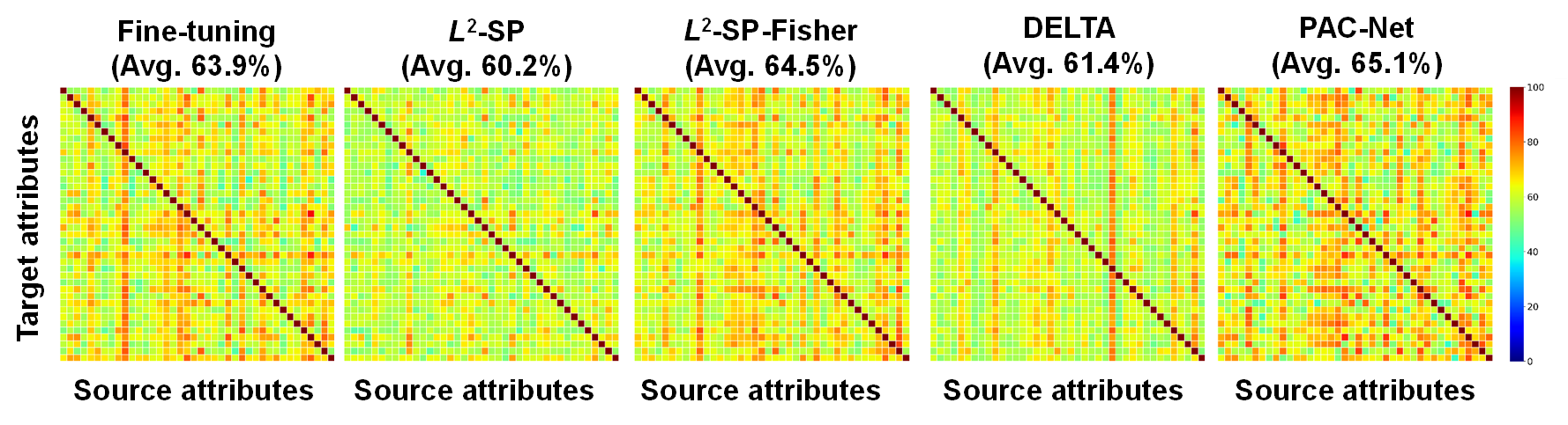
Figure 3: Accuracy of the multiple algorithms with 50 target samples between individual attributes on the CelebA dataset. PAC-Net clearly shows the best performance in varying the attributes between the source and the target. Each attribute is in alphabetical order and is not indicated for readability.

We further conducted an ablation study to appreciate each steps of pruning, allocation, and calibration in PAC-Net. Isolating each step yields the following algorithms:

• PC-Net: We fix $\mathbf{w}_{U}$ collected by pruning and we calibrate $\mathbf{w}_{P}$ to the target task while skipping the allocation step, i.e., $\mathbf{w}_{U}$ is NOT updated.

• PAC-Net (No-$L^{2}$): We calibrate $\mathbf{w}_{P}$ to the target task without $L^{2}$ regularization. This is essentially PackNet (Mallya & Lazebnik, 2018).

• PAC-Net (RI): We initialize $\mathbf{w}_{P}$ to random values in the calibration step.

• PA-Net-$L^{2}$-SP or PA-Net-$L^{2}$-SP-Fisher: After the pruning and allocation steps, we do not fix $\mathbf{w}_{U}$ but calibrate all weights to the target task with soft ($L^{2}$-SP) or semi-hard regularization ($L^{2}$-SP-Fisher).

Table 2 summarizes the whole ablation studies. Comparing PAC-Net to PC-Net, we confirmed the importance of keeping the complete source knowledge. This result is consistent with $L^{2}$-SP and $L^{2}$-SP-Fisher that partially forget the source knowledge. As a result compared to PAC-Net (No-$L^{2}$), we proved it is crucial to regularize $\mathbf{w}_{P}$ although preserving the source knowledge. Consistent with the hypothesis of $L^{2}$-SP, zero SP of $\mathbf{w}_{P}$ shows the better performance than the random SP of $\mathbf{w}_{P}$ (PAC-Net (RI)).

4.2 Classification

CelebFaces Attributes Dataset (CelebA) (Liu et al., 2018b) is a large-scale celebrity images with the forty attribute annotations. For the source task, we trained the ResNet-18 (He et al., 2016) with one attribute as a binary classification, and then fitted the trained model to the target tasks with different attributes by varying the number of target samples. Table 3 is an example describing whether the model that trains an eyeglasses attribute can help to train the arched eyebrow attribute, or vice versa. The baseline algorithms for comparison are fine-tuning, $L^{2}$-SP, $L^{2}$-SP-Fisher, and DELTA (Li et al., 2019). Our method shows the better performance than others. For all the forty attributes, we examined the performance of different approaches for the binary classification tasks. Figure 3 clearly indicates our method outperforms other algorithms.

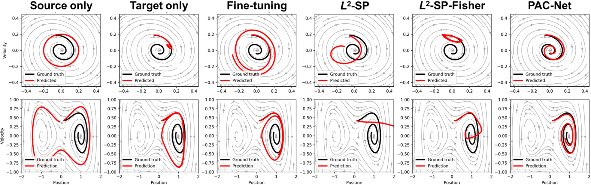
Figure 4: Phase plot of the multiple algorithms with Neural ODE for linear oscillator (top) and non-linear oscillator (bottom). The linear and non-linear oscillator are the results with three and eight target samples, respectively. PAC-Net can calibrate the discrepancy between the source and the target while others cannot.

Table 4: RMSE results of multiple inductive transfer learning algorithms with Neural ODE model on Duffing equation. PAC-Net shows the lowest error in most experiments.

System	Method	10	20	30	40	50	60	70	80	90	100	Avg.
Linear	Target only	2.85	3.30	0.54	0.42	0.36	0.84	0.16	0.10	0.09	0.06	0.87
	Fine-tuning	3.88	0.53	0.60	0.18	0.12	0.05	0.05	0.03	0.02	0.02	0.55
	$L^{2}$-SP	0.84	0.77	0.68	0.65	0.58	0.58	0.57	0.57	0.56	0.52	0.63
	$L^{2}$-SP-Fisher	3.43	0.82	0.23	0.18	0.07	0.05	0.06	0.05	0.07	0.04	0.5
	PAC-Net	0.19	0.11	0.06	0.05	0.05	0.05	0.04	0.04	0.03	0.03	0.07
Non-linear	Target only	3.23	3.40	1.49	0.85	1.18	1.05	1.07	0.51	0.44	0.33	1.36
	Fine-tuning	0.73	2.16	0.62	0.85	0.31	0.41	0.26	0.24	0.25	0.19	0.60
	$L^{2}$-SP	0.84	1.59	1.70	1.91	1.86	2.21	2.24	2.38	1.93	2.12	1.88
	$L^{2}$-SP-Fisher	3.46	1.56	1.10	1.04	1.39	1.52	1.15	1.15	0.49	0.4	1.33
	PAC-Net	0.92	0.76	0.64	0.65	0.22	0.21	0.20	0.21	0.20	0.20	0.42

4.3 Ordinary Differential Equations

We introduce another task obeying ordinary differential equations as the real-world scenario. We introduce Duffing oscillator (Kovacic & Brennan, 2011) given by:

$$\frac{d\mathbf{q}}{dt}=\mathbf{p},\frac{d\mathbf{p}}{dt}=-\alpha\mathbf{q}-\beta\mathbf{q}^{3}-\gamma\mathbf{p}$$

where $\alpha,\beta$, and $\gamma$ are the calibration parameters that control the linear stiffness, the amount of non-linearity in the restring force, and the amount of damping, respectively. $\mathbf{p}$ and $\mathbf{q}$ are position and velocity, respectively. There are two system, linear and non-linear oscillator for inductive transfer learning problems.

Linear oscillator.

We choose a linear oscillator, i.e., $\alpha=1,\beta=0,\gamma=0$ in the source task and $\alpha=1,\beta=0,\gamma=0.3$ in the target task, respectively.

Non-linear oscillator.

As the more complex problem, we introduced the non-linear oscillator, i.e., $\alpha=-1,\beta=1,\gamma=0$ in the source task and $\alpha=-1,\beta=1,\gamma=0.3$ in the target task, respectively.

With two oscillation systems, the source task denotes the energy conservation system and the target task the energy loss system caused by the frictional force, as described in Section 1. In this task, we should infer the trajectory in the reality (target task) after the observed trajectory within a few seconds. The leftmost of Figure 4 shows the discrepancy between the simulation (source) and experiment (target). Note that as a base learner, we employed a Neural ODE (Chen et al., 2018) to predict the trajectory. Figure 4 depicts PAC-Net can well calibrate the target task based on the source task while others cannot. Table 4 describes RMSE of the target trajectory. PAC-Net predicts the most accurate trajectory in both systems over most experiments that varies the number of target data.

4.4 Partial Differential Equations

We evaluate PAC-Net with real-world scenarios in which the discrepancy between the simulation and reality should be close. The diffusion equation is one of PDEs with various applications. We choose the equation with Dirichlet boundary condition, as follows:

$$\begin{split}&\partial_{t}u(x,y,t)=v\Delta u(x,y,t),x,y\in(0,2),t\in(0,1]\\ &\text{subject to initial condition:}\\ &u(x,y,0)=\begin{cases}2&\text{if 0.5 $<$ x, y $<$ 1}\\ 1&\text{Otherwise}\end{cases}\\ &\text{and boundary condition:}\\ &u(0,y,t)=u(2,y,t)=u(x,0,t)=u(x,2,t)=1,\end{split}$$ (6)

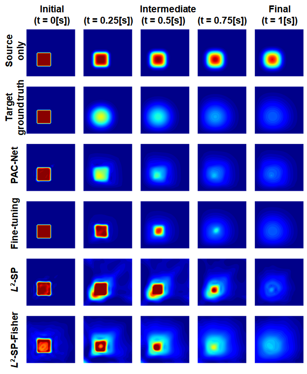
Figure 5: Diffusion flows of various algorithms with PINN as time advances. PAC-Net accurately predicts the concentration flows at a intermediate time, which has never been so far.

Table 5: RMS error on diffusion equation in the target task.

Method	0.25 [s]	0.5 [s]	0.75 [s]	1.0 [s]	Avg.
Fine-tuning	0.164	0.104	0.028	0.001	0.074
$L^{2}$-SP	0.396	0.310	0.132	0.023	0.215
$L^{2}$-SP-Fisher	0.192	0.162	0.108	0.089	0.138
PAC-Net	0.056	0.039	0.020	0.006	0.030

where $u$ denotes the concentration, $v$ is an unknown parameter that can vary with the materials. We set $v$ to be 0.01 and 0.1 for the source and target task, respectively. With only initial and the boundary conditions (6) in the source task, we trained a physics-informed neural network (PINN) (Raissi et al., 2019), which learns PDEs of (6). As a realistic scenario(Myung et al., 2021a), we assume that final concentration data with the unknown $v$ is only available so that we make model predict a concentration profile at intermediate steps. As shown in Figure 5, the concentration for target task shows a considerable discrepancy with that for source task. We fitted PINN that learned the diffusion equation in the source task to the initial and final concentration in the target task with various inductive transfer learning algorithms. Figure 5 clearly shows that PAC-Net can predict the target data at intermediate step while others do not. Table 5 shows the mean-squared error as time advances, which depicts PAC-Net outperforms others.

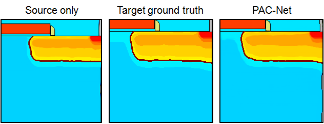
Figure 6: Prediction results with 40 target samples.

4.5 Real-world Problem

In this section, we introduce semiconductor dataset, as a real-world problem that experiences a difference between reality and simulation. The dataset consists of the scalar values as an input and images as an output. We used the RTT model (Myung et al., 2020, 2021b) to solve this problem. The left and the center of Figure 6 illustrate the outputs of source and target tasks can differ although the input features are the same. Table 6 shows PAC-Net works well even when only 40 target samples are available in training. Figure 6 indicates that PAC-Net can clearly predict the target task.

Table 6: Results with RTT model on semiconductor dataset.

Method	20	40	60	80	100
Target only	0.703	0.799	0.855	0.883	0.893
PAC-Net	0.884	0.907	0.924	0.932	0.933

5 Conclusion

Inductive transfer learning aims to resolve the distributional shift problem with a little target data while there exists enough amount of source data. Consistent with previous studies, we found the importance of preserving source knowledge. $L^{2}$-SP, DELTA, and PAC-Net aim to preserve the knowledge in source tasks while solving the aforementioned problem by taking different approaches. $L^{2}$-SP imposes the regularization to all weights to preserve the source knowledge, and DELTA additionally applies channel-wise attention to feature maps. On the other hand, PAC-Net encourages updating the insignificant weights while keeping the source weights. Experimental results show that PAC-Net is more effective than competitive baseline methods.

Appendix A Experiment Details

A.1 Regression

Architectural Details.

We used two fully-connected layers with output size of 200 with ReLU activation, and one fully-connected layer as the prediction function with linear activation. All layers are initialized with he normal (He et al., 2015), and the mean-squared error is used as loss function with a batch size of 128 where Adam optimizer (Kingma & Ba, 2015) is performed with the step size $10^{-4}$. For TradaBoost.R2 (Pardoe & Stone, 2010), which is available on the website, we choose the two-stage version with 10 first stage and five second stage iterations. For $L^{2}$-SP, we choose the regularization parameter to 0.01. For PAC-Net, we set pruning ratio to 0.8 and $\lambda$ to 0.01.

Experiment Details.

We carried out five experiments as follows: i) there are 20,000 datasets, half of which are training sets, and the rest are test sets. ii) input features of both domains are same. iii) target training datasets vary in size. Note that the source model is fixed in every iteration adding target samples.

A.2 CelebA

Architectural Details.

We used ResNet-18 architecture. For $L^{2}$-SP and PAC-Net, we regularized the weights of all convolution layers with the penalty of each method. We imposed no regularization to the dense layer for PAC-Net while applying $L^{2}$ regularization whose strength is 0.01 to the dense layer for $L^{2}$-SP. For fine-tuning, we fitted all weights based on the source weights. The parameters we used are as follows: the loss function is cross-entropy, the optimizer Adam with the step size $10^{-4}$, batch size 128. For PAC-Net, we set pruning ratio to 0.8 and $\lambda$ to 0.01. For $L^{2}$-SP, we set the $L^{2}$ strength of convolution layers to 0.01.

Experiment Details.

We resized the image to 64x64. For an experiment, we selected each 2000 images for source and target. Also, we randomly picked another 2000 images from the rest of attributes (38 attributes) for model to learn generic knowledge regrading datasets. We used a half of the images for the train dataset and the rest for the test dataset. We repeated the experiments five times with the different random seeds.

A.3 Ordinary Differential Equations

Architectural Details.

We used six fully-connected layers with output size of 256 with tanh activation, and one fully-connected layer as the prediction function with linear activation. For Neural ODE (Chen et al., 2018) solver, we used adaptive Runge-Kutta (RK) methods (Hairer et al., 1993). The parameters we used are as follows: the loss function is mean-squared error, the optimizer Adam with the step size $10^{-4}$, batch size 512. For PAC-Net, we set pruning ratio to 0.8 and $\lambda$ to 0.001. For $L^{2}$-SP, we set the regularization parameter to 0.001.

Experiment Details.

This experiment is similar with (Huh et al., 2020). From equation 1, we generated 100 and 10 trajectories whose time interval is 0.1 for source and target dataset, respectively. For each trajectory, the initial state $(\mathbf{q}(t_{0}),\mathbf{p}(t_{0}))$ is uniformly sampled from annulus in [0.2, 1]. For the target task, we added uniformly distributed noise multiplied by 0.01 for each trajectory. With ten trajectories for target task, we assessed the RMSE losses of the trajectories from one second to ten second.

A.4 Partial Differential Equations

Architectural Details.

We used six fully-connected layers with output size of 256 with swish activation (Ramachandran et al., 2017), and one fully-connected layer as the prediction function with linear activation. When training the source task, we used the particular loss function that (PINN, (Raissi et al., 2019)) proposed, as follows:

For the target task, we used mean-squared-error to fit the model with an available target data. The parameters we used are as follows: the optimizer is Adam with the step size $10^{-4}$, batch size 32. For PAC-Net, we set pruning ratio to 0.8 and $\lambda$ to 0.01. For $L^{2}$-SP, we set the $L^{2}$ strength to 0.01.

A.5 Real-world Problem

Dataset Description.

We briefly introduce semiconductor process dataset, sampled by Technology Computer-Aided Design (TCAD, (Synopsys, 2009)). The input features are 17 dimensions and consist of two types; the first is the features related to structure, and the other is related to the profile. Figure 7 presents the result of process simulator, explaining that the size of the doping profile depends on input features. Since structure-related features such as $L_{G}$ and $T_{OX}$ make the image size varying, we put padding area to maintain the fixed size. The profile-related features, the lower part of the image, also affect the color, which means when the yellow part shrinks, the blue part expands, or vice versa. All output images are added to padding to meet the images 320x320 size.

Experiment Details.

Our experiment procedures are as follows: i) we trained the baseline models with 1,000 source data, ii) the number of target samples varied in size, iii) we assessed the performance of the methods with 51 target samples that domain engineers consider importantly.

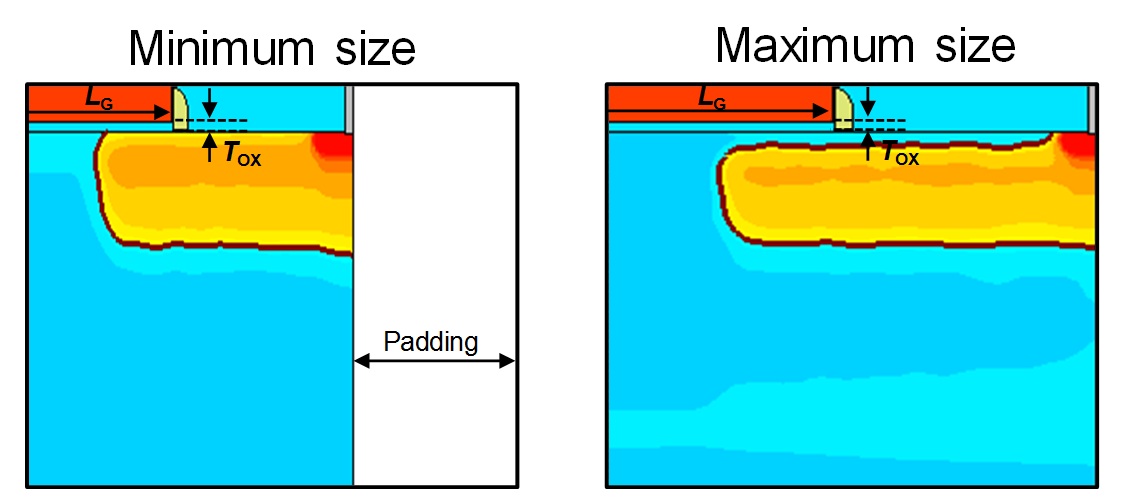
Figure 7: Description of semiconductor datasets.

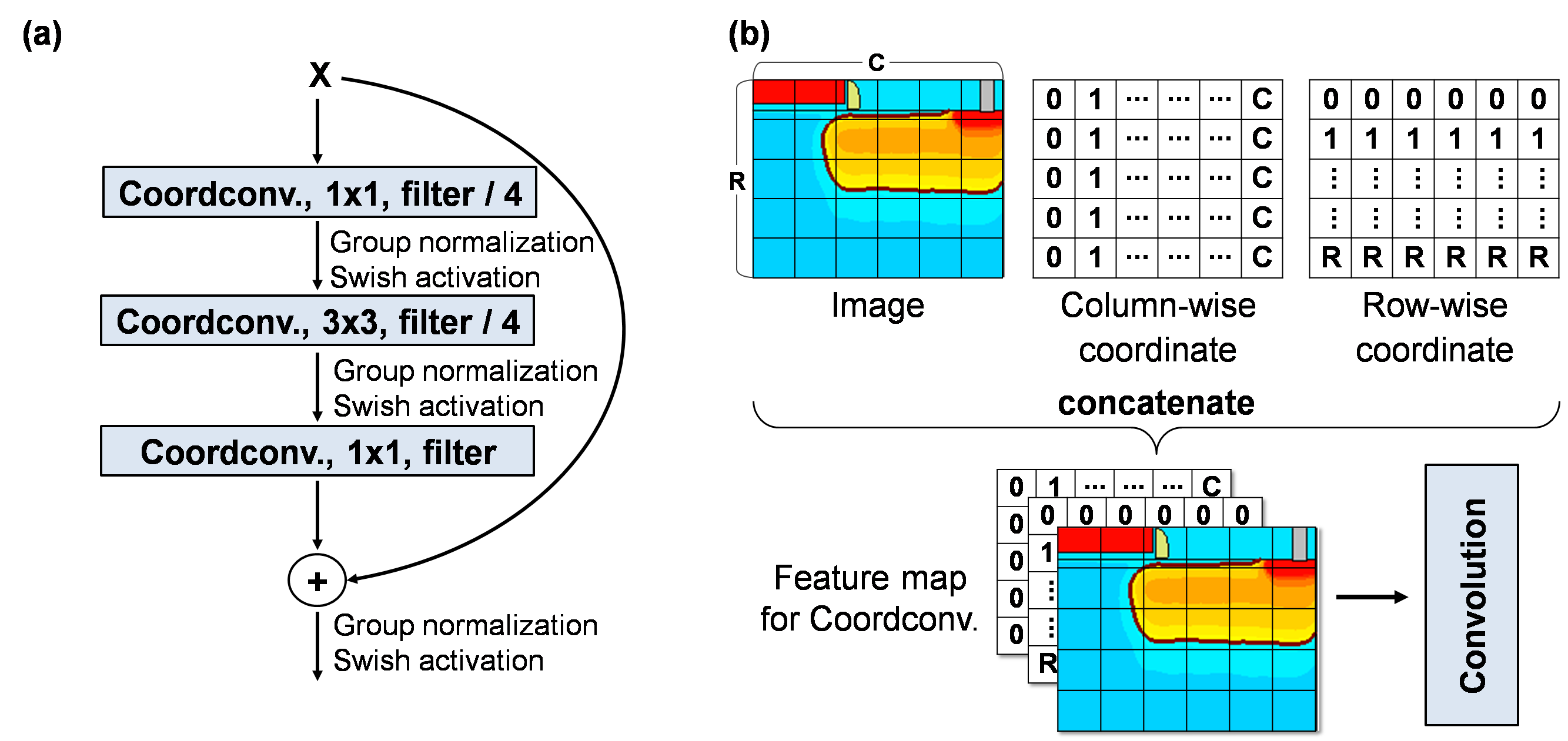
Figure 8: Description of the baseline model on semiconductor dataset. (a) Illustration of components of the residual block. (b) Description of coordinate convolution.

Architectural detail.

We used RTT model (Myung et al., 2020, 2021b). The model is based on residual blocks ((He et al., 2016)), which consist of coordinate convolution ((Liu et al., 2018a)), swish activation ((Ramachandran et al., 2017)), and group normalization ((Wu & He, 2018)) as depicted in Figure 8. The model is trained for 10,000 epochs with a batch size of 128, where Adam optimizer is performed with the step size $10^{-4}$. For PAC-Net, we set pruning ratio is 0.8 and $\lambda=0.01$.

References

- Ajakan et al. (2014) Ajakan, H., Germain, P., Larochelle, H., Laviolette, F., and Marchand, M. Domain-adversarial neural networks. arXiv preprint arXiv:1412.4446, 2014.
- Chen et al. (2020) Chen, S., Hou, Y., Cui, Y., Che, W., Liu, T., and Yu, X. Recall and learn: Fine-tuning deep pretrained language models with less forgetting. In Proceedings of the 2020 Conference on Empirical Methods in Natural Language Processing (EMNLP), pp. 7870–7881, 2020.
- Chen et al. (2018) Chen, T. Q., Rubanova, Y., Bettencourt, J., and Duvenaud, D. K. Neural ordinary differential equations. In NeurIPS, 2018.
- Chen et al. (2019) Chen, X., Wang, S., Fu, B., Long, M., and Wang, J. Catastrophic forgetting meets negative transfer: Batch spectral shrinkage for safe transfer learning. Advances in Neural Information Processing Systems, 32:1908–1918, 2019.
- Frankle & Carbin (2019) Frankle, J. and Carbin, M. The lottery ticket hypothesis: Finding sparse, trainable neural networks. In International Conference on Learning Representations, 2019.
- Freund & Schapire (1997) Freund, Y. and Schapire, R. E. A decision-theoretic generalization of on-line learning and an application to boosting. Journal of Computer and System Sciences, 55(1):119–139, 1997.
- Gouk et al. (2020) Gouk, H., Hospedales, T. M., and Pontil, M. Distance-based regularisation of deep networks for fine-tuning. arXiv preprint arXiv:2002.08253, 2020.
- Hairer et al. (1993) Hairer, E., Nørsett, S. P., and Wanner, G. Solving ordinary differential equations. 1, Nonstiff problems. Springer-Vlg, 1993.
- Han et al. (2015) Han, S., Pool, J., Tran, J., and Dally, W. J. Learning both weights and connections for efficient neural networks. In Advances in Neural Information Processing Systems, pp. 1135–1143, 2015.
- Han et al. (2017) Han, S., Pool, J., Narang, S., Mao, H., Gong, E., Tang, S., Elsen, E., Vajda, P., Paluri, M., Tran, J., et al. DSD: Dense-sparse-dense training for deep neural networks. In International Conference on Learning Representations, 2017.
- Hassibi et al. (1993) Hassibi, B., Stork, D., and Wolff, G. Optimal brain surgeon: Extensions and performance comparisons. Advances in neural information processing systems, 6, 1993.
- He et al. (2015) He, K., Zhang, X., Ren, S., and Sun, J. Delving deep into rectifiers: Surpassing human-level performance on imagenet classification. In Proceedings of the IEEE international conference on computer vision, pp. 1026–1034, 2015.
- He et al. (2016) He, K., Zhang, X., Ren, S., and Sun, J. Deep residual learning for image recognition. In Proceedings of the IEEE conference on computer vision and pattern recognition, pp. 770–778, 2016.
- Huh et al. (2020) Huh, I., Yang, E., Hwang, S. J., and Shin, J. Time-reversal symmetric ode network. Advances in Neural Information Processing Systems, 33:19016–19027, 2020.
- Kingma & Ba (2015) Kingma, D. P. and Ba, J. Adam: A method for stochastic optimization. In ICLR (Poster), 2015.
- Kovacic & Brennan (2011) Kovacic, I. and Brennan, M. J. The Duffing equation: nonlinear oscillators and their behaviour. John Wiley & Sons, 2011.
- LeCun et al. (1990) LeCun, Y., Denker, J. S., and Solla, S. A. Optimal brain damage. In Advances in neural information processing systems, pp. 598–605, 1990.
- Li & Zhang (2021) Li, D. and Zhang, H. Improved regularization and robustness for fine-tuning in neural networks. Advances in Neural Information Processing Systems, 34, 2021.
- Li et al. (2018) Li, X., Grandvalet, Y., and Davoine, F. Explicit inductive bias for transfer learning with convolutional networks. In International Conference on Machine Learning, pp. 2825–2834. PMLR, 2018.
- Li et al. (2019) Li, X., Xiong, H., Wang, H., Rao, Y., Liu, L., Chen, Z., and Huan, J. Delta: Deep learning transfer using feature map with attention for convolutional networks. arXiv preprint arXiv:1901.09229, 2019.
- Li et al. (2020) Li, X., Grandvalet, Y., and Davoine, F. A baseline regularization scheme for transfer learning with convolutional neural networks. Pattern Recognition, 98:107049, 2020.
- Liu et al. (2018a) Liu, R., Lehman, J., Molino, P., Such, F. P., Frank, E., Sergeev, A., and Yosinski, J. An intriguing failing of convolutional neural networks and the coordconv solution. arXiv preprint arXiv:1807.03247, 2018a.
- Liu et al. (2018b) Liu, Z., Luo, P., Wang, X., and Tang, X. Large-scale celebfaces attributes (celeba) dataset. Retrieved August, 15(2018):11, 2018b.
- Lubana & Dick (2020) Lubana, E. S. and Dick, R. A gradient flow framework for analyzing network pruning. In International Conference on Learning Representations, 2020.
- Malach et al. (2020) Malach, E., Yehudai, G., Shalev-Schwartz, S., and Shamir, O. Proving the lottery ticket hypothesis: Pruning is all you need. In International Conference on Machine Learning, pp. 6682–6691, 2020.
- Mallya & Lazebnik (2018) Mallya, A. and Lazebnik, S. Packnet: Adding multiple tasks to a single network by iterative pruning. In Proceedings of the IEEE/CVF Conference on Computer Vision and Pattern Recognition, pp. 7765–7773, 2018.
- McCloskey & Cohen (1989) McCloskey, M. and Cohen, N. J. Catastrophic interference in connectionist networks: The sequential learning problem. In Psychology of Learning and Motivation, volume 24, pp. 109–165. Elsevier, 1989.
- Motiian et al. (2017) Motiian, S., Piccirilli, M., Adjeroh, D. A., and Doretto, G. Unified deep supervised domain adaptation and generalization. In Proceedings of the IEEE International Conference on Computer Vision, pp. 5715–5725, 2017.
- Myung et al. (2020) Myung, S., Kim, J., Jeon, Y., Jang, W., Huh, I., Kim, J., Han, S., h. Baek, K., Ryu, J., Kim, Y. S., Doh, J., h. Kim, J., Jeong, C., and Kim, D. S. Real-time TCAD: a new paradigm for tcad in the artificial intelligence era. In International Conference on Simulation of Semiconductor Processes and Devices (SISPAD), pp. 347–350, 2020.
- Myung et al. (2021a) Myung, S., Jang, H., Choi, B., Ryu, J., Kim, H., Park, S. W., Jeong, C., and Kim, D. S. A novel approach for semiconductor etching process with inductive biases. arXiv preprint arXiv:2104.02468, 2021a.
- Myung et al. (2021b) Myung, S., Jang, W., Jin, S., Choe, J. M., Jeong, C., and Kim, D. S. Restructuring tcad system: Teaching traditional tcad new tricks. In 2021 IEEE International Electron Devices Meeting (IEDM), pp. 18–2. IEEE, 2021b.
- Pan & Yang (2009) Pan, S. J. and Yang, Q. A survey on transfer learning. IEEE Transactions on Knowledge and Data Engineering, 22(10):1345–1359, 2009.
- Pardoe & Stone (2010) Pardoe, D. and Stone, P. Boosting for regression transfer. In International Conference on Machine Learning, pp. 863–870, 2010.
- Raissi et al. (2019) Raissi, M., Perdikaris, P., and Karniadakis, G. E. Physics-informed neural networks: A deep learning framework for solving forward and inverse problems involving nonlinear partial differential equations. Journal of Computational Physics, 378:686–707, 2019.
- Rajpurkar et al. (2016) Rajpurkar, P., Zhang, J., Lopyrev, K., and Liang, P. Squad: 100,000+ questions for machine comprehension of text. arXiv preprint arXiv:1606.05250, 2016.
- Ramachandran et al. (2017) Ramachandran, P., Zoph, B., and Le, Q. V. Searching for activation functions. arXiv preprint arXiv:1710.05941, 2017.
- Sun & Saenko (2016) Sun, B. and Saenko, K. Deep coral: Correlation alignment for deep domain adaptation. In Proceedings of the European Conference on Computer Vision, pp. 443–450, 2016.
- Synopsys (2009) Synopsys. Sentaurus Process user’s manual, 2009.
- Tzeng et al. (2017) Tzeng, E., Hoffman, J., Saenko, K., and Darrell, T. Adversarial discriminative domain adaptation. In Proceedings of the IEEE/CVF Conference on Computer Vision and Pattern Recognition, pp. 7167–7176, 2017.
- Wu & He (2018) Wu, Y. and He, K. Group normalization. In Proceedings of the European Conference on Computer Vision, pp. 3–19, 2018.
- Xu et al. (2019) Xu, X., Zhou, X., Venkatesan, R., Swaminathan, G., and Majumder, O. d-sne: Domain adaptation using stochastic neighborhood embedding. In Proceedings of the IEEE/CVF Conference on Computer Vision and Pattern Recognition, pp. 2497–2506, 2019.
- Yan et al. (2017) Yan, H., Ding, Y., Li, P., Wang, Q., Xu, Y., and Zuo, W. Mind the class weight bias: Weighted maximum mean discrepancy for unsupervised domain adaptation. In Proceedings of the IEEE/CVF Conference on Computer Vision and Pattern Recognition, pp. 2272–2281, 2017.
- Yao & Doretto (2010) Yao, Y. and Doretto, G. Boosting for transfer learning with multiple sources. In Proceedings of the IEEE/CVF Conference on Computer Vision and Pattern Recognition, pp. 1855–1862, 2010.
- Yosinski et al. (2014) Yosinski, J., Clune, J., Bengio, Y., and Lipson, H. How transferable are features in deep neural networks? In Advances in Neural Information Processing Systems, pp. 3320–3328, 2014.
- Zellinger et al. (2017) Zellinger, W., Grubinger, T., Lughofer, E., Natschläger, T., and Saminger-Platz, S. Central moment discrepancy (CMD) for domain-invariant representation learning. In International Conference on Learning Representations, 2017.
- Zhang et al. (2021) Zhang, Z., Jin, J., Zhang, Z., Zhou, Y., Zhao, X., Ren, J., Liu, J., Wu, L., Jin, R., and Dou, D. Validating the lottery ticket hypothesis with inertial manifold theory. Advances in Neural Information Processing Systems, 34, 2021.