RL-GA: A Reinforcement Learning-Based Genetic Algorithm for Electromagnetic Detection Satellite Scheduling Problem

Abstract

The study of electromagnetic detection satellite scheduling problem (EDSSP) has attracted attention due to the detection requirements for a large number of targets. This paper proposes a mixed-integer programming model for the EDSSP problem and a genetic algorithm based on reinforcement learning (RL-GA). Numerous factors that affect electromagnetic detection are considered in the model, such as detection mode, bandwidth, and other factors. The RL-GA embeds a Q-learning method into an improved genetic algorithm, and the evolution of each individual depends on the decision of the agent. Q-learning is used to guide the population search process by choosing evolution operators. In this way, the search information can be effectively used by the reinforcement learning method. In the algorithm, we design a reward function to update the Q value. According to the problem characteristics, a new combination of $<$state, action$>$ is proposed. The RL-GA also uses an elite individual retention strategy to improve search performance. After that, a task time window selection algorithm (TTWSA) is proposed to evaluate the performance of population evolution. Several experiments are used to examine the scheduling effect of the proposed algorithm. Through the experimental verification of multiple instances, it can be seen that the RL-GA can solve the EDSSP problem effectively. Compared with the state-of-the-art algorithms, the RL-GA performs better in several aspects.

1 Introduction

In recent years, the rapid development of aerospace has provided new solutions for various types of tasks such as information communication, environmental monitoring, and disaster forecasting[1]. The applications that satellites can play can be divided into three categories: observation, communication, and navigation according to the different carrying payloads. Here, observation satellites can be further classified according to the payload equipped with visible light, infrared, synthetic aperture radar, antenna, and others. Satellites that use signal receivers and antennas as payloads are called electromagnetic detection satellites. Electromagnetic detection satellites can detect and process electromagnetic signals to obtain helpful information. Compared with optical imaging satellites, electromagnetic detection satellites have a wider detection range and are not easily affected by weather factors. As a result, it can execute tasks in all types of weather conditions. Based on known signal characteristics, electromagnetic detection satellites can also search for unknown signals through a wide range of frequencies.

There are a large number of electromagnetic signals on the surface of the earth, and many types of electromagnetic signals constitute the surface electromagnetic environment together. The detection of surface electromagnetic environments can effectively support work in various fields such as environment, agriculture, military, meteorology, and others. The electromagnetic detection satellite scheduling problem (EDSSP) is to plan the satellite resources used to execute the demand and determine the specific execution time of each task. Detection demands are put forward by various users and are expected to be met fully. However, the tasks that can be performed during each orbit are quite limited. This is due to the existence of limitations such as satellite orbit, detection range, and operating conditions. The goal of electromagnetic detection satellite scheduling is to generate a reasonable task sequence within a certain time range. This sequence is expected to generate sufficient detection profit and satisfy users’ preferences. While the characteristic of oversubscription is very common in a satellite scheduling problem. How to build a model and design a scheduling algorithm then becomes the most central issue.

Electromagnetic signal detection needs to effectively balance the relationship between the detection accuracy and the satellite capability. From the signal detection activity itself, when the density of detection frequency points is increased to improve the detection accuracy, the amount of data generated will also increase accordingly. The capacity of the onboard storage device is limited. If the storage device is fully used, it will not be possible to execute a new task until it is erased. The reasonable setting of detection accuracy according to user needs can improve detection performance.

Existing studies of electromagnetic detection satellite mission planning have proposed corresponding solution methods for multiple scenarios such as multiple area detection and moving target detection[2, 3]. However, the specific modes of satellites are treated in a simplified way in these studies, which only addresses the problem that is common to all types of satellite scheduling problems. It can be said that these studies are not mature and in-depth enough. Compared with the electromagnetic detection satellite scheduling problem, there are many studies related to the optical satellite observation scheduling problem[4, 5]. In terms of model building, Berger and Barkaoui used the quadratic programming method to construct the visible light satellite scheduling model[6, 7]. Cho et al. proposed a two-step binary linear programming model to formulate a satellite observation scheme for a low-orbit satellite constellation[8]. Niu et al. considered using satellites to complete post-disaster large-area observation tasks built a multi-objective optimization model and used genetic algorithms to solve this problem[9]. Chen et al. proposed a mixed-integer programming model for the agile satellite scheduling problem, constructing decision variables based on conflicts between time windows and using 5-index variables to obviate the need for a Big-M approach[10].

Evolutionary algorithms have been widely used in solving satellite task scheduling problems. The applications of the genetic algorithm[11], differential evolution[12], ant colony algorithm[13], memetic algorithm[14] and others algorithms have increased rapidly in recent years. Compared with accurate algorithms, the evolutionary algorithm has a lower computational cost on large-scale problems. The studies of [15, 16] show that genetic algorithms are more suitable for solving satellite task scheduling problems than other evolutionary algorithms. E. et al. proposed an individual reconfiguration-based integer coding genetic algorithm (IRICGA) for regional target observation planning and designed a new area partitioning method based on two kinds of discrete parameters[17]. Zhang and Xing adopted a novel idea of encoding and decoding for the integrated satellite imaging and data transmission scheduling problem to improve the search efficiency of the genetic algorithm. Two test cases are used to verify the algorithm effect [18]. Song et al. and Du et al. used non-dominated sorting-based and decomposition-based multi-objective evolutionary algorithms, respectively, to find high-quality solutions for satellite range scheduling problems[19, 20]. Xhafa et al. proposed a genetic algorithm combined with the STK solution tool to obtain a plan of ground stations[21].

Existing research on reinforcement learning to solve satellite scheduling problems rarely considers combining it with other algorithms. Solving this problem using the reinforcement learning method alone is also just beginning. Wei et al. directly used reinforcement learning methods to solve imaging satellite scheduling problems[22]. Chen et al. built an end-to-end reinforcement learning framework, used the attention mechanism, and proposed an actor-critic network training method[23]. To the best of our knowledge, there is no research that the embedded approach to solving the satellite scheduling problem.

Combining reinforcement learning with search algorithms can effectively utilize the respective advantages of the two methods to improve search efficiency and search performance [24]. A part of the related research focuses on numerical optimization problems[25, 26].

Rodríguez-Esparza et al. [27] used a hyper-heuristic algorithm consisting of a multi-armed bandit RL method and a simulated annealing algorithm to solve the path planning problem for electric vehicles with capacity constraints. This hyper-heuristic algorithm uses RL to select a neighborhood search strategy and obtains a legal route by repairing the solution. Zhang et al. [28] proposed an improved algorithm combining the Q-learning method and multi-objective particle swarm algorithm for the multi-UAV path planning problem. This algorithm uses a deep reinforcement learning method to determine the mode used for particle swarm search. Du et al [29] considered the effect of electricity cost in a flexible job shop scheduling problem and proposed a reinforcement learning-based distribution estimation algorithm. The algorithm uses DQN to select the rules for process adjustment. Half of the individuals are constituted in this way and the other half is optimized by the distribution estimation algorithm.

These combined methods above achieve good performance and demonstrate the advantages of this algorithm design idea. For the EDSSP problem, we try to use a new combination of a genetic algorithm and reinforcement learning method to find the ideal plan. Control parameters are extremely important for each evolutionary algorithm, and these parameters are always sensitive to the problem. This easily affects the generalization of the algorithm. The reinforcement learning method has strong generalization capabilities but is prone to poor performance due to a lack of domain-specific knowledge. So, we try to apply the reinforcement learning method to the evolutionary algorithm and effectively combine the respective advantages of these two methods.

Our proposed reinforcement learning-based genetic algorithm allows researchers to invest more effort in algorithm and strategy design. The reinforcement learning approach helps the genetic algorithm find higher-quality solutions through intelligent decision-making. Such an approach has strong application prospects and can effectively deal with various types of complex situations. For the method, this is the first time that reinforcement learning is used to embed into an evolutionary algorithm for solving a satellite scheduling problem, and this research idea can also be applied to other combinatorial optimization problems.

The main contributions of our research are:

1. A refined model of the EDSSP problem is built. This mixed-integer programming model considers many practical factors such as detection mode, detection angle, and data volume, which is conducive to obtaining a more practical scheduling scheme.

2. A genetic algorithm based on reinforcement learning is proposed. The algorithm uses a reinforcement learning method to drive the population search. Combining the problem characteristics of EDSSP, we construct a new combination of state and action methods and propose a reward function and strategy selection method. In addition, a two-stage task time window selection algorithm is proposed. It is used to generate detection schemes and calculate the fitness function values.

3. The effectiveness of the proposed RL-GA is verified by extensive experiments. The RL-GA is excellent in terms of solution performance and can solve large-scale EDSSP effectively. It also provides an idea for solving other combinatorial optimization problems.

The remainder of this paper is organized as follows. The second part introduces the model of the electromagnetic detection satellite scheduling problem. The third part introduces the reinforcement learning-based genetic algorithm and the task time window selection algorithm. The fourth part verifies the effect of the proposed algorithm. The fifth part summarizes the content and analyzes possible directions for further research in the future.

2 Model

2.1 Problem Description

The EDSSP problem is to designate a time-ordered task execution sequence for electromagnetic detection satellites. The goal is to maximize the detection sequence profit while satisfying various satellite constraints. For a satellite to successfully perform any mission, it needs to determine the on/off time of the receiver i.e. the start time and the end time of the mission. A series of parameter settings such as detection mode, frequency, bandwidth, and polarization mode must also be followed.

The time range from the beginning to the end of the signal beam coverage of the electromagnetic satellite is called the visible time window. Since the electromagnetic satellite antenna can effectively detect a wide range of ground signals, to reduce noise and improve the detection accuracy, the angle between the signal source and the pointing direction of the satellite antenna needs to be within a certain range.

The detection quality is affected by two factors. On the one hand, the signal gain is affected by the angular relationship between the satellite antenna and the signal source. When the center of the satellite antenna passes directly above the signal source, the maximum signal gain can be obtained, and the signal gain is directly linked to the detection profit. Signal gain is inversely related to the angle between the antenna and the signal source. In other words, when the centerline of the signal source beam coincides with the extension line of the satellite antenna pointing direction, the detection effect is the best. On the other hand, the detection accuracy will also affect the detection profit. The detection accuracy is limited by the inherent capability of the receiver, and the number of frequency points will also have a direct impact on the detection accuracy. There is a positive correlation between the bandwidth and the number of frequency points, and the amount of data obtained by detection varies significantly depending on settings. The limited satellite storage capacity means that only a fraction of tasks can be set to the highest bandwidth, while many tasks need to be set to a smaller bandwidth.

2.2 Symbols and Variables

$T$ : Set of tasks, a total of ${\left|T\right|}$ tasks. For task $task_{j}$, the following attributes are defined:

$es{t_{j}}$: The earliest available start time of the task.

$le{t_{j}}$: The latest available end time of the task.

$du{r_{j}}$: Duration of the task.

$\theta_{j}^{\max}$: Maximum allowable detection angle of the task.

$degre{e_{j}}$ : Task importance level.

${m_{j}}$: The amount of data for the task.

${G_{j}}$: The signal gain can be obtained from the task.

$S$: Set of satellites, a total of ${\left|S\right|}$ satellites. For satellite ${s_{i}}$, the following attributes are defined:

$D$: Satellite antenna diameter.

$\eta$ : Antenna efficiency.

${O_{i}}$: Set of Orbits, a total of $\left|{{O_{i}}}\right|$ orbits belonging to satellite ${s_{i}}$.

$\beta$ : Satellite detection unit data volume.

$M$: Satellite storage capacity.

${\Gamma_{pol}}$ : Satellite polarization transition time.

${\Gamma_{mode}}$ : Satellite detection mode transition time.

${\Gamma_{band}}$: Satellite bandwidth setting transition time.

${\Gamma_{fre}}$: Satellite frequency band transition time.

$\Delta$ : Satellite load on/off time.

$TW$ : Set of time windows, with a total of $\left|{TW}\right|$ time windows. For the time window $t{w_{ijok}}$, the following attributes are defined:

$EV{T_{ijok}}$ : The earliest visible time of the task $j$ in the time window $k$ on orbit $o$ for satellite $i$.

$LV{T_{ijok}}$ : The latest visible time of the task $j$ in the time window $k$ on orbit $o$ for satellite $i$.

$\theta_{{}_{ijok}}^{t}$ : Detection angle of the satellite $i$ at the time $t$ in the time window $k$ of the task $j$ on the orbit $o$.

$I$: A big integer.

Decision variables:

${x_{ijok}}$ : Whether the satellite $i$ is in the time window $k$ on the orbit $o$ whether the task $j$ is executed, if the task is executed, ${x_{ijok}}=1$; otherwise, ${x_{ijok}}=0$.

$s{t_{ijo}}$ : Start time of the satellite $i$ on the orbit $o$ to execute the task $j$.

2.3 Mathematical Model

We refer to the studies of [30] and [31] and make the following assumptions.

Assumptions:

• All electromagnetic detection satellites have the same receivers and storage devices;

• The detection process will not be affected by external factors;

• The detection task is definite, and there will be no temporary changes or cancellations;

• The satellite has sufficient energy during orbit;

• Each task can be completed after one detection, without repeated detection.

The calculation formula of the detection profit that can be obtained by a single detection task is:

$${G_{j}}={G_{0}}\cdot{\left[{\frac{{{J_{1}}\left(u\right)}}{{2u}}+36\frac{{{J_{3}}\left(u\right)}}{{{u^{3}}}}}\right]^{2}}\left({dBi}\right)$$ (1)

$${G_{0}}=\eta\frac{{{\pi^{2}}{D^{2}}}}{{{\lambda^{2}}}}\left({dBi}\right)$$ (2)

where $u=2.07123\sin\left(\theta\right)/\sin\left({{\theta_{3dB}}}\right)$, ${{J_{1}}\left(u\right)}$ and ${{J_{3}}\left(u\right)}$ are the 1st and 3rd order Bessel functions of the first kind, respectively. $\theta$ is the angle between the satellite antenna and the center of the signal source, $\theta_{3dB}$ is the angle at which the antenna gain is attenuated by 3dB relative to the center of the beam, and the calculation formula as follows.

$${\theta_{3dB}}=70\lambda/D$$ (3)

where $\lambda$ represents the wavelength, and $D$ indicates the diameter of the antenna.

In this paper, the bandwidth used by satellites to perform detection tasks is dynamically matched according to the priority of detection tasks. The importance of the task is high, and the bandwidth used is large so that the detection effect will be better. However, due to the limitation of satellite storage, the detection bandwidth needs to be scientifically set. The formula for setting the bandwidth according to the degree of importance ${degre{e_{j}}}$ is shown below.

$$\varphi\left({degre{e_{j}}}\right)=\left\{{\begin{array}[]{*{20}{c}}{bandwidt{h_{1}}}&{degre{e_{j}}>75}\\ {bandwidt{h_{2}}}&{50<degre{e_{j}}\leq 75}\\ {bandwidt{h_{3}}}&{25<degre{e_{j}}\leq 50}\\ {bandwidt{h_{4}}}&{0<degre{e_{j}}\leq 25}\end{array}}\right.$$ (4)

The bandwidth setting can also affect the detection profit, and the signal gain can be measured by the function $\Omega\left[{\varphi\left({degre{e_{j}}}\right)}\right]$. When the bandwidth of the detection task $j$ is set according to $\varphi\left({degre{e_{j}}}\right)$, the amount of data generated per second is $\beta\cdot\varphi\left({degre{e_{j}}}\right)$. Combined with the task detection time $du{r_{j}}$, the total data amount of task $j$ can be obtained by:

$${m_{j}}=\beta\cdot\varphi\left({degre{e_{j}}}\right)\cdot du{r_{j}}$$ (5)

The main parameters of the electromagnetic detection task include frequency, bandwidth, polarization, and detection mode. The parameters of satellite $s_{i}$ for task $task_{j}$ are set as $\left(fre_{ij},band_{ij},pol_{ij},mode_{ij}\right)$. Where $fre_{ij}$ denotes the detection frequency, $band_{ij}$ denotes the bandwidth, $pol_{ij}$ denotes the polarization mode, and $mode_{ij}$ denotes the detection mode. The electromagnetic detection satellite needs to adjust the parameters of the onboard equipment when performing different tasks. The transition time between tasks is composed of four parts. The first part is the time required for the change of the polarization mode. The second part is the time required for the change of the detection mode. The third part is the time required for the change of the frequency, and the fourth part is the time required for the change of the bandwidth. In addition, it also takes a certain amount of time for each onboard equipment to be turned on and off, and this time interval $\delta$ must be satisfied between every two tasks. To simplify the constraint judgment, we introduce a new variable $tra{n_{ijj^{\prime}}}$, which represents the total transition time. The transition time of the two tasks $j$ and ${j^{\prime}}$ is as follows.

$$\begin{array}[]{l}tra{n_{ijj^{\prime}}}=\max\left\{{{\Gamma_{fre}}\left({fr{e_{ij}},fr{e_{ij^{\prime}}}}\right),0,\Delta}\right.{\Gamma_{band}}\left({ban{d_{ij}},ban{d_{ij^{\prime}}}}\right),{\Gamma_{pol}}\left({po{l_{ij}},po{l_{ij^{\prime}}}}\right)\\ \left.{{\Gamma_{mode}}\left({mod{e_{ij}},mod{e_{ij^{\prime}}}}\right)}\right\}\end{array}$$ (6)

where ${\Gamma_{pol}}$ is the satellite polarization transition time, ${\Gamma_{mode}}$ is the satellite detection mode transition time, ${\Gamma_{band}}$ is the satellite bandwidth setting transition time, ${\Gamma_{fre}}$ is the satellite frequency transition time, $\Delta$ is the satellite load on/off time.

The scheduling goal of the EDSSP problem is to obtain the highest detection profit. The objective function is represented as follows.

Objective function:

$$\max\sum\limits_{i\in S}{\sum\limits_{j\in T}{\sum\limits_{o\in{O_{i}}}{\sum\limits_{k\in TW}{{G_{j}}}}}}\cdot\Omega\left[{\varphi\left({degre{e_{j}}}\right)}\right]\cdot{x_{ijok}}$$ (7)

where ${G_{j}}$ is signal gain can be obtained from the task, $\Omega\left[{\varphi\left({degre{e_{j}}}\right)}\right]$ is the gain due to the bandwidth setting, the product of ${G_{j}}$ and $\Omega\left[{\varphi\left({degre{e_{j}}}\right)}\right]$ represents the profit of the task.

Constraints:

$$s{t_{ijo}}\geq es{t_{j}}\cdot{x_{ijok}},\forall i\in S,j\in T,o\in{O_{i}},k\in TW$$ (8)

$$\left({s{t_{ijo}}+du{r_{j}}}\right)\cdot{x_{ijok}}\leq le{t_{j}},\forall i\in S,j\in T,o\in{O_{i}},k\in TW$$ (9)

$$\theta_{{}_{ijok}}^{t}\leq\theta_{j}^{\max},\forall i\in S,j\in T,o\in{O_{i}},k\in TW,t\in\left[{s{t_{ijo}},s{t_{ijo}}+du{r_{j}}}\right]$$ (10)

$$s{t_{ijo}}\geq EV{T_{ijok}}\cdot{x_{ijok}},\forall i\in S,j\in T,o\in{O_{i}},k\in TW$$ (11)

$$\begin{array}[]{l}\left({s{t_{ijo}}+du{r_{j}}}\right)\cdot{x_{ijok}}\leq LV{T_{ijok}},\forall i\in S,j\in T,o\in{O_{i}},k\in TW\end{array}$$ (12)

$$\begin{array}[]{*{20}{c}}{\sum\limits_{i\in S}{\sum\limits_{j\in T\backslash\left\{{j^{\prime}}\right\}}{\sum\limits_{k\in TW}{{m_{j}}\cdot{x_{ijok}}}}}+{m_{j^{\prime}}}\cdot{x_{ij^{\prime}ok^{\prime}}}\leq M}{,\forall i\in S,j\in T,o\in{O_{i}},k\in TW}\end{array}$$ (13)

$$\begin{array}[]{*{20}{c}}{\left({s{t_{ijo}}+du{r_{j}}}\right)\cdot{x_{ijok}}+tra{n_{ijj^{\prime}}}\leq s{t_{ij^{\prime}o}}+I\cdot\left({1-{x_{ij^{\prime}ok^{\prime}}}}\right)}{,j\neq j^{\prime},i\in S,j\in T,o\in{O_{i}},k\in TW}\end{array}$$ (14)

$$\sum\limits_{i\in S}{\sum\limits_{o\in{O_{i}}}{\sum\limits_{k\in TW}{{x_{ijok}}}}}\leq 1,\forall i\in S,o\in{O_{i}},k\in TW$$ (15)

$${x_{ijok}}\in\left\{{0,1}\right\}$$ (16)

Constraints 1-2 indicate that the start time and end time of the task must be within the time range required. Constraint 3 indicates that the detection angle cannot exceed the task maximum angle requirement. Constraints 4-5 indicate that the start time and end time are within the visible time window. Constraint 6 indicates that the satellite cannot exceed the upper limit of the satellite storage capacity in each orbit. Constraint 7 indicates that the satellite must meet various transition time requirements to perform every two tasks. Constraint 8 indicates that each task can be executed at most once. Constraint 9 indicates the value range of the decision variable.

3 The Proposed Method

Since the single satellite imaging scheduling problem has been proved to be NP-hard, the more complex EDSSP problem does not exist polynomial time algorithm[33, 34]. Therefore, we propose a reinforcement learning-based genetic algorithm to solve the EDSSP problem. In addition, we also design a task time window selection algorithm for generating schemes. The reinforcement learning-based genetic algorithm, details in evolutionary algorithms, and strategies in reinforcement learning and task time window selection algorithms are given in this section.

3.1 Reinforcement Learning based Genetic Algorithm (RL-GA)

Input: population size ${N_{p}}$, learning rate $\alpha$, discount factor $\gamma$, Q-table $Q$, $\varepsilon$, control parameter $T$, crossover operator ${C_{o}}$, mutation operator ${M_{o}}$, $L$

Output: ${Solution}$

1 Initialize algorithm parameters and the population;

2 Set $t=1$, $num\_eval=0$, $local\_best=0$, $count=0$, $global\_best=0$, $global\_best_{i}ndividual=\left[\ \right]$, $local\_best\_individual=\left[\ \right]$;

3 Initialize Q-table${(C_{o},M_{o})}$;

4 while $num\_eval<MFE$ do

5       for $p=1$ to ${N_{p}}$ do

6             $\rho\left({{s_{i}},{a_{j}}}\right)\leftarrow$Use softmax strategy$\left({{Q_{t}}\left({{s_{i}},{a_{j}}}\right),T}\right)$;

7             $A_{p}^{t}\leftarrow$Select action with Q-Learning$\left(\varepsilon,\rho\left({{s_{i}},{a_{j}}},T\right)\right)$;

8             ${indi_{p}^{t-1}}\leftarrow$Roulette selection of individual $\left({P_{t-1}},{F_{t-1}}\right)$;

9             ${indi_{p}^{t}}\leftarrow$Evolution Operation$\left({indi_{p}^{t-1}},A_{p}^{t}\right)$// A combination of crossover and mutation operators;

10             ${S_{p}^{t}}\leftarrow$Generate a plan$\left(indi_{p}^{t},T,TW\right)$ //Use Task Time Window Selection Algorithm;

11             ${F_{p}^{t}}\leftarrow$Fitness Evaluation$\left({S_{p}^{t}}\right)$ by Eq. 7;

12             ${R_{t}}\leftarrow$Compute Reward$\left({F_{t}},{F_{t-1}}\right)$ by Eq. 18;

13             ${Q_{t+1}}\leftarrow$Compute Q-values$\left({{S_{t}},{A_{t}}},{R_{t}},\alpha,\gamma\right)$;

14             $t\leftarrow t+1$;

15             ${num\_eval}\leftarrow num\_eval+1$;

16            

17      

18      ${local\_best}\leftarrow$Find the max fitness of current population$\left(P_{t}\right)$;

19       if $local\_best>global\_best$ then

20             $global\_best\leftarrow local\_best$;

21             $global\_best\_individual\leftarrow local\_best\_individual$;

22      else

23             if $count$ not equal to $Thre$ then

24                   //Retain elite individuals

25                   $P_{t}\leftarrow$ Replace the individual of $selected\_id$ with $gobal\_best\_individual$;

26                  

27            

28      if $local\_best<=last\_local\_best$ then

29             $count\leftarrow count+1$;

30            

31      $last\_local\_best\leftarrow local\_best$;

32      

Algorithm 1 Reinforcement Learning based Genetic Algorithm (RL-GA)

Evolutionary algorithms simulate the evolution process of biological populations and find high-quality solutions to problems in the form of population evolution. Population search brings a strong global search capability to evolutionary algorithms, which ensures its performance in solving large-scale complex problems.

The obvious disadvantage of evolutionary algorithms is that the search results are extremely sensitive to the parameter configuration. This feature makes many evolutionary algorithms have dependencies on specific problems and scenarios. When problems or scenarios change, parameters need to be adjusted or reset. The parameter tuning process is time-consuming. According to the characteristics of the evolutionary algorithm and reinforcement learning method, we design a reinforcement learning-based genetic algorithm for the EDSSP problem. Genetic algorithm has good global search ability, and it has a good performance in the field of sequence optimization and scheduling, such as traveling salesman problems, vehicle route planning problems, satellite task scheduling problems, and many other problems. To improve the local search ability of the genetic algorithm, we introduce the elite individual retention strategy into the genetic algorithm. RL-GA uses a Q-learning method to complete the evolution of the population. The Q-learning method is responsible for selecting crossover and mutation operations. The population obtained by the RL-GA algorithm uses a task time window selection algorithm (TTWSA) to complete the decoding and generate the task execution plan. The profit obtained by the TTWSA is used for the reward calculation and then the Q value update process. In other words, TTWSA provides a basis for the learning method to select new actions. The pseudo-code of the genetic algorithm based on Q-learning is shown in Algorithm Table 2.

In RL-GA, $count$ is a parameter to control whether the algorithm executes elite individual retention. When $count$ is equal to $Thre$ (Line 22), elite individuals are no longer retained. Obtaining the task planning scheme from the genetic algorithm needs to use the task time window selection algorithm. The TTWSA can determine the tasks that can be executed and determine the specific start time and end time. Figure 1 shows the dataflow between the reinforcement learning method and the genetic algorithm population search.

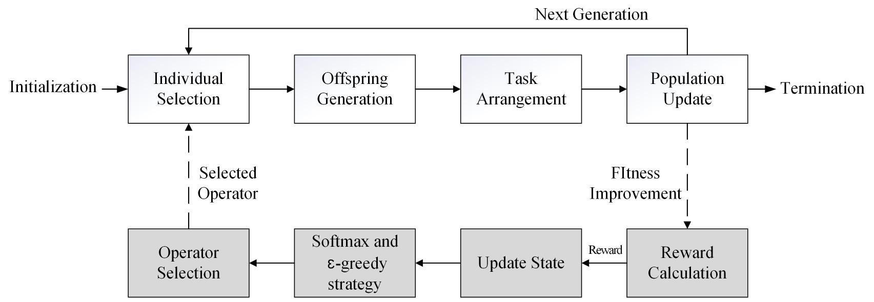
Figure 1: Dataflow between the RL method and GA

As shown in Figure 1, the top row of the figure represents the GA population evolution process, and the bottom row represents the Q-learning algorithm choosing the operator, updating the state, etc. It can be seen from the figure that there is a close connection between GA and Q-learning method. The GA provides data input for the agent to select actions, and the actions selected by the agent are used directly in the population evolution.

3.1.1 Individual Representation and Initialization

The initialization method is the first step in the population search to obtain a detection scheme. It needs to construct an initial solution in a certain way and further search to find a higher-quality solution based on the initial solution. In the RL-GA, individuals are encoded in real numbers. For decoding, the RL-GA uses the task time window selection algorithm to determine whether to execute each task according to the order of tasks. If one task can be executed, the specific execution time of the task will be determined. Otherwise, the task will be discarded. Eventually, the scheme will be generated by arranging the tasks one by one. The advantage of real number coding is to ensure the unique correspondence between the elements at each position in the sequence, and the decoding process is simple. Another benefit of this individual representation method is that it effectively guarantees the legitimacy of the solution structure without using any repair methods.

3.1.2 Fitness Evaluation

Fitness evaluation method has two roles in the RL-GA algorithm, one is to select individuals from the population, and the other is to evaluate the reward and update state in the reinforcement learning method. The fitness evaluation is obtained by calculating the objective function value of each corresponding to the plan by Eq. 7. The method for generating plans from individuals is introduced in section 3.3.

3.1.3 Individual Selection

Individual selection is the premise of population evolution. After an individual is selected, the corresponding operation chosen by the reinforcement learning method can be completed to obtain a new individual. On the one hand, individual selection should make good performers more likely to be successfully selected. On the other hand, other individuals should also have a certain possibility of being selected to ensure the diversity of the population. Therefore, we use a roulette approach to select an individual in the RL-GA. The calculation formula for selecting individuals by roulette is as follows.

$${p_{i}}=\frac{{fi{t_{i}}}}{{\sum\limits_{i=1}^{N_{p}}{fi{t_{i}}}}}$$ (17)

where ${fi{t_{i}}}$ represents the fitness function value of individual. The fitness function value is calculated using Eq. 7.

3.1.4 Crossover

The purpose of evolution is to improve the performance of individuals within a population. We use crossover and mutation operators to search for good detection plans. For the crossover operation in the RL-GA, we design seven crossover operators with various lengths and heuristic rules, which are called short segment crossover operator (denoted as C1), medium segment crossover operator (denoted as C2), and long segment crossover operator (denoted as C3), segment flip (denoted as C4), foremost position crossover (denoted as C5), segment internal order adjustment based on earliest available start time (denoted as C6), fragment internal order adjustment based on task duration (denoted as C7).

Short segment crossover operator (C1): Short segment crossover refers to selecting two task sequence segments of length $L$ from an individual and exchanging the positions of the two segments in the individual. The schematic diagram of the short segment crossover is shown in Figure 2.

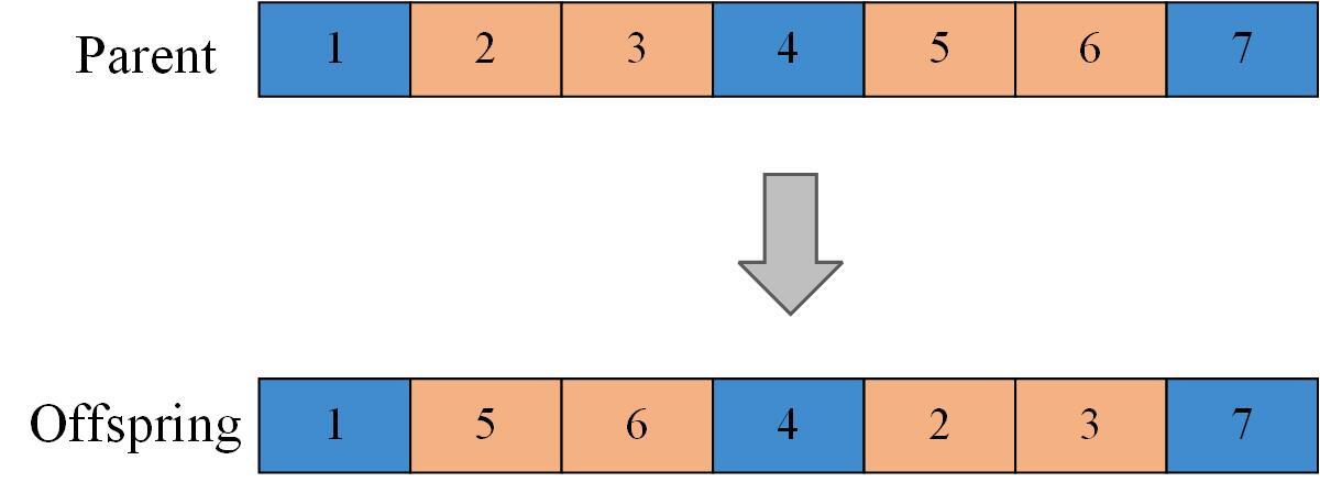
Figure 2: Schematic Diagram of the Short Segment Crossover

Medium segment crossover operator (C2): Medium segment crossover refers to selecting two task sequence segments of length $2L$ from an individual and swapping the positions of the two segments in the individual.

Long segment crossover operator (C3): Long segment crossover refers to selecting two task sequence segments of length $3L$ from an individual and exchanging the positions of the two segments in the individual.

Fragment flipping (C4): Fragment flipping is to select a task sequence fragment of length $L$ from an individual and rearrange the task sequence from back to front. The schematic diagram of the fragment flipping is shown in Figure 3.

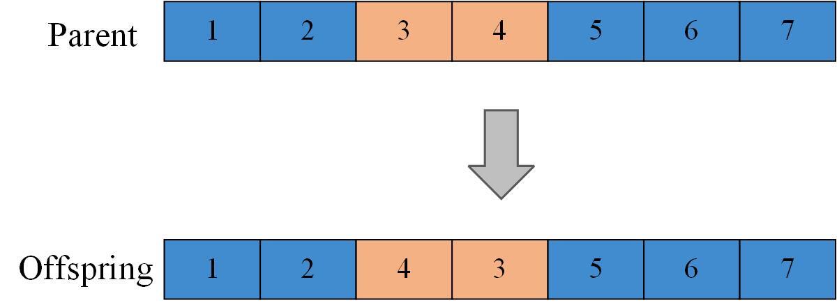
Figure 3: Schematic Diagram of the Fragment Flipping

Foremost position crossover (C5): Select a task sequence segment of length $L$ from an individual, and swap the segment with the task sequence segment of the same length at the foremost position of the individual.

Segment internal order adjustment based on earliest available start time (C6): Select a task segment of length $L$ from an individual and adjust the internal segment order from front to back according to its task’s earliest available start time $est_{j}$.

Segment internal order adjustment based on task duration (C7): Select a task segment of length $L$ from an individual and adjust the internal segment sequence from short to long according to the task required duration $dur_{j}$.

3.1.5 Mutation

Compared with crossover, the variation degree of mutation is smaller, which is also helpful for improving the search performance. The mutation in RL-GA is performed by exchanging two positions in the sequence. We combine the crossover operator and mutation operator to complete the individual evolution of the population. After the evolution process is completed, the fitness of offspring needs to be evaluated. The TTWSA is used to generate a plan and the fitness value of each individual is calculated by Eq. 7. In the RL-GA, the crossover and mutation operators used for optimization are chosen by the Q-learning method, and the operation used for individual evolution is selected according to the Q value.

3.1.6 Reinforcement Learning Method

We adopt the Q-learning method to guide the search for an evolutionary algorithm. Q-learning is a simple and effective reinforcement learning method, which is widely used in various models such as DQN and DRL according to the actions taken by the algorithm adaptive decision-making according to the Q value[35, 36]. Q-learning consists of five parts: action, state, reward, learning algorithm, and environment, which can be represented as a quadruple of $\left\langle{A,S,R,L,E}\right\rangle$[37]. The state of the agent indicates whether the fitness function value has improved through the search, and is divided into two states, one with improvement and the other without improvement or reduction. Such a state representation can be associated with the improvement of the population fitness value or can be combined with optional actions to form a Q-table. In this way, the Q-table is simple and can be closely integrated with the population evolution process. The actions represent the combination of population search operators used, consisting of several crossover and mutation operators.

The Q-learning method selects the population update strategy through the update of the Q value, which replaces the traditional operator selection method in the evolutionary algorithm. More specifically, the agent selects the appropriate operator for population evolution based on the Q-value and action selection strategy. The interaction between the agent and the environment is evaluated by the reward function. The reward value is closely related to the fitness value and fitness improvement. The running process of Q-learning is shown in Figure 4.

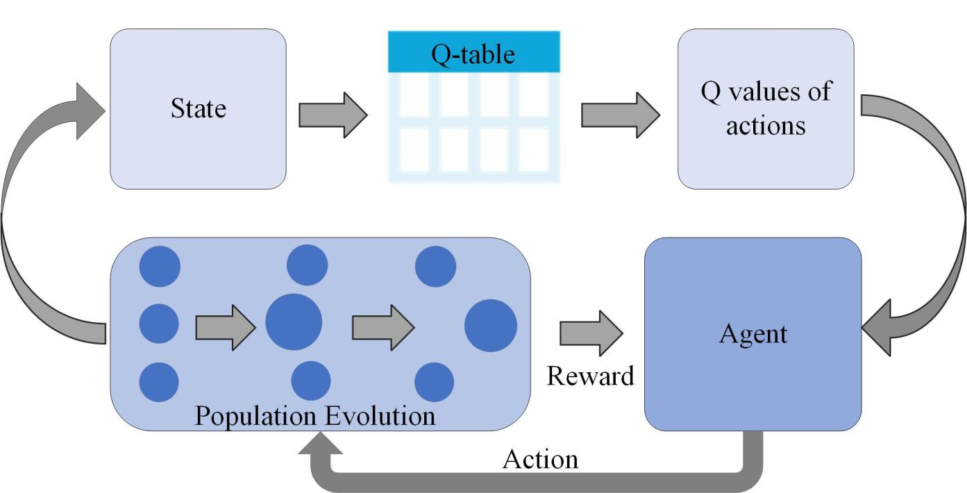
Figure 4: Q-learning Method Decision-making Process for EDSSP

As shown in Figure 4, the RL-GA algorithm generates offspring after each population evolution search using the operators decided by the Q-learning method. And the task time window selection algorithm is used to generate detection plans. The value of the fitness function can be easily calculated based on the plan. The Q-learning method can further obtain fitness improvement. The state will update according to the fitness improvement.

The formula for calculating reward is shown below.

$${R_{t}}={F_{t}}\left({{S_{t}},A_{t}}\right)-{F_{t-1}}\left({{S_{t-1}},A_{t-1}}\right)$$ (18)

where ${F_{t}}$ and ${F_{t-1}}$ are values of fitness at the time $t$ and $t-1$, respectively.

The updated formula for the Q value is shown below.

$$\begin{array}[]{l}{Q_{t+1}}\left({{S_{t}},{A_{t}}}\right)={Q_{t}}\left({{S_{t}},{A_{t}}}\right)+\alpha\left({{R_{t}}+\gamma\mathop{\max}\limits_{a}{\rm{}}Q\left({{S_{t+1}},a}\right)-{Q}\left({{S_{t}},{A_{t}}}\right)}\right)\end{array}$$ (19)

where $\alpha$ is the learning rate, and $\gamma$ is the discount factor.

An important part of Q-learning is the Q-value table, which records the performance values of all crossover and mutation combinations used in the search process. When the RL-GA algorithm contains ${n_{c}}$ kinds of crossover operators and ${n_{m}}$ kinds of mutation operators, the total number of actions contained in the Q-value table is ${n_{c}}\times{n_{m}}+{n_{c}}+{n_{m}}$. In our proposed algorithm, there are 7 kinds of crossover operators and 1 kind of mutation operator. Therefore, the number of actions that each agent can choose is 15. We set the state to two levels according to the fitness function value improvement, which is higher (denoted as I) and lower (denoted as II). In the proposed algorithm, the number of $<$state, action$>$ combinations is 30. For each agent, the probability of selecting $a_{j}$ action in state $s_{i}$ is usually determined by Softmax strategy:

$$\rho\left({{s_{i}},{a_{j}}}\right)=\frac{{{e^{{{{Q_{t}}\left({{s_{i}},{a_{j}}}\right)}\mathord{\left/{\vphantom{{{Q_{t}}\left({{s_{i}},{a_{j}}}\right)}T}}\right.\kern-1.2pt}T}}}}}{{\sum\nolimits_{j=1}^{n}{{e^{{{{Q_{t}}\left({{s_{i}},{a_{j}}}\right)}\mathord{\left/{\vphantom{{{Q_{t}}\left({{s_{i}},{a_{j}}}\right)}T}}\right.\kern-1.2pt}T}}}}}}$$ (20)

where ${{Q_{t}}\left({{s_{i}},{a_{j}}}\right)}$ is the corresponding value in the Q table at time $t$, and $T$ is a control parameter.

Due to the large value of the objective function in the EDSSP problem, the introduction of a control parameter $T$ can effectively prevent the probability value of individuals from being too large. Meanwhile, the reinforcement learning method needs to balance the exploration and exploitation of algorithm[10]. To prevent the algorithm from falling into a local optimum that is difficult to jump out, we use a parameter $\varepsilon$ to regulate this process. When the randomly generated probability value is less than $\varepsilon$, a random evolution strategy is selected to generate offspring.

3.1.7 Elite Individual Retention Strategies

Since the EDSSP problem has a large solution space, we use an elite individual retention strategy in the RL-GA to improve the convergence performance. When the retention process occurs, the optimal individual obtained by the search is retained in the next generation population. The use of elite individuals will affect the global search ability of the algorithm after a certain period of search. Therefore, we introduce a parameter $count$ and a threshold $Thre$. When the current population search is not improved compared to the previous generation population, i.e., the maximum fitness value of the population does not change. The parameter $count$ will increase by 1. If the value of parameter $count$ is equal to the threshold $Thre$, the elite individual is no longer retained.

3.1.8 Termination

After a certain number of iterative searches, the RL-GA needs to finish the search process and output the optimal result as the final execution plan. Since we adopt the crossover and mutation operators based on reinforcement learning, when the agent chooses an action, it can correspond to one or two evolution operations. Therefore, it is reasonable to use the evolution times $num\_eval$ as the evaluation index to record the iterative search. When the algorithm evolution times reach the set maximum evolution times $MFE$, the algorithm search process will be terminated.

3.2 Task Time Window Selection Algorithm (TTWSA)

When the task execution is determined through algorithm optimization, the start time and end time of the task need to be determined. The TTWSA algorithm tries to schedule the tasks in the best position to obtain the maximum detection profit and adjusts the execution time of the tasks according to the actual situation faced. The heuristic rules used in the algorithm refer to the approach used in [31, 32] and are designed accordingly to the EDSSP problem. The setting of task start time and end time not only affects the detection profit of the task but also affects the satisfaction of constraints. We propose a two-stage task time window selection algorithm with preliminary filtering and then determine the execution time. The purpose of preliminary filtering is to ensure that the task execution can meet the requirements of constraints, such as angle, transition time, and others. Therefore, the preliminary filtering needs to clip some time windows that do not meet the constraints or discard the current time window and try to schedule tasks in another time window. The basis of preliminary filtering is to obtain the actual earliest actual available start time ${AEV{T_{ijok}}}$ and the latest actual available end time ${ALV{T_{ijok}}}$. The preliminary filtering is based on the Eq. 10-12. The formulas of ${AEV{T_{ijok}}}$ and ${ALV{T_{ijok}}}$ are shown as Eq. 21 and Eq. 22 respectively.

$$AEV{T_{ijok}}=\max\left\{{es{t_{j}},EV{T_{ijok}}}\right\}$$ (21)

$$ALV{T_{ijok}}=\min\left\{{le{t_{j}},LV{T_{ijok}}}\right\}$$ (22)

After the preliminary filtering, the algorithm can specify the start time and end time of the task. Detection profit that can be obtained follows the rule of first growing and then decreasing. To obtain more profit, the detection process should ensure that the angle between the antenna and the signal source is as small as possible. The time range in which the algorithm chooses to execute the task should allow for sufficient profit. Generally speaking, the change in the angle between the satellite and the target in the time window can be regarded as a symmetrical process. Therefore, the middle position of the time window is the best choice as an intermediate moment, which usually has the smallest angle. And the start execution time and the task end time are determined according to this intermediate moment. The formula for calculating the best start time is as follows.

$$bst_{ijo}=\left(EVT_{ijok}+LVT_{ijok}\right)/2-dur_{j}/2$$ (23)

$$be{t_{ijo}}=bs{t_{ijo}}+du{r_{j}}$$ (24)

where $bs{t_{ijo}}$ represents the best start time of the execution task $j$ of satellite $i$ on orbit $o$.

If this moment can meet the requirements of other constraints, it will be regarded as the final start time; otherwise, move the execution time backward or forward until all constraints are met. The pseudo-code of the task time window selection algorithm is shown in the Algorithm Table 2.

Input: Task Set ${T}$, Time Window ${TW}$, Detection Task Sequence ${indi_{p}^{t}}$

Output: Solution $S_{i}^{t}$

1foreach task ${t_{i}}$ in ${T}$ in the order in ${indi_{p}^{t}}$ do

2       foreach time window ${tw_{j}}$ in ${TW}$ do

3             ${AEV{T_{ijok}}=\max\left\{{es{t_{j}},EV{T_{ijok}}}\right\}}$ ;

4             ${ALV{T_{ijok}}=\min\left\{{le{t_{j}},LV{T_{ijok}}}\right\}}$ ;

5             if ${(ALV{T_{ijok}}-AEV{T_{ijok}})\geq d}$  then

6                   $bs{t_{ijo}}\leftarrow$Calculate the best start time by Eq. LABEL:best_start_time;

7                   $be{t_{ijo}}\leftarrow$Calculate the best end time by Eq. 24;

8                   if $bs{t_{ijo}}<AEV{T_{ijok}}$ then

9                         $s{t_{ijo}}\leftarrow$ move backward to determine start time;

10                        

11                  if $be{t_{ijo}}>ALV{T_{ijok}}$ then

12                         $s{t_{ijo}}\leftarrow$ move forward to determine start time;

13                        

14                  $t{w^{\prime}_{j}},t{w^{\prime\prime}_{j}}\leftarrow$Update ${tw_{j}}$;

15                   $TW\leftarrow$ Add $t{w^{\prime}_{j}}$ and $t{w^{\prime\prime}_{j}}$ into $TW$;

16                   $TW\leftarrow$Omit ${tw_{j}}$ from $TW$;

17                   Try to arrange next task ${t_{i+1}}$;

18                  

19            else

20                   Turn to next time window $tw_{j+1}$;

21                  

22            

23      

Algorithm 2 Task Time Window Selection Algorithm

4 Performance Evaluation of Proposed Algorithm

4.1 Experimental Settings

The configuration of the experiment in this paper is Core I7-7700 3.6 GHz CPU, 16 GB memory, Windows 11 operating system desktop computer, and Matlab 2020a is used for coding. All algorithms are run under the same system configuration.

We use a series of Chinese satellites for our experiments. The satellite orbit parameters can be defined by a hexagram: the length of semi-major axis $\left(a\right)$, eccentricity $\left(e\right)$, inclination $\left(i\right)$, argument of perigee $\left(\omega\right)$, right ascension of the ascending node $\left(\varphi\right)$, and mean anomaly $\left(m\right)$. Table 1 gives the initial orbital parameters of two satellites.

Table 1: Initial Orbital Parameters of Two Satellites

Satellite	$a$	$e$	$i$	$\omega$	$\varphi$	$m$
No. 1	7000	0.00015	97.672	0	21.75	158.25
No. 2	7000	0.00015	97.672	0	51.75	128.25
…	…	…	…	…	…	…

We use AGI Systems Tool Kit (STK) 11.2 to generate the task and time window data needed for scheduling. The task distribution is randomly generated on a global scale. The planning time horizon of the tasks is all within one day. For a detection task, the duration follows a uniform distribution in the interval $\left[10,100\right]$ seconds, and the mission requires a maximum time horizon of 12 hours to execute. Each task is completed with only one detection activity by satellite. When the bandwidth used by the satellite is set to $bandwidth_{1}$, $bandwidth_{2}$, $bandwidth_{3}$, $bandwidth_{4}$, and $bandwidth_{5}$, the signal gains obtained obey a uniform distribution in the intervals $\left[1,3\right]$, $\left[4,6\right]$, $\left[7,9\right]$, $\left[10,12\right]$, and $\left[13,15\right]$, respectively.

To verify the effect of our proposed algorithm. We choose an improved genetic algorithm (IGA)[38], an adaptive large neighborhood search algorithm (ALNS/TPF)[39], an artificial bee colony algorithm (ABC) [40], and a construction heuristic algorithm (CHA) as state-of-the-art algorithms. The IGA algorithm adopts a heuristic mechanism and uses knowledge to guide the algorithm search. The ALNS/TPF algorithm combines tabu search and adaptive large neighborhood search algorithm to find high-quality solutions through destruction and repair. The ABC algorithm search solution space (also known as nectar sources) through three types of bees, imitating the way bee populations search. The CHA algorithm gives the planned task sequence according to the way of sorting the task profit. The above four algorithms have a large number of applications in satellite task scheduling problems and other planning problems and have good performance.

The evaluation times $MFE$ of all algorithms were set to 5000 times. The control parameter $T$ of RL-GA is set to 1000, the initial learning rate $\alpha$ is set to 0.01, the discount factor $\gamma$ is set to 0.95, the threshold $Thre$ is set to 100, the length $L$ is 2 and $\varepsilon$ is 0.01. The crossover probability of the IGA algorithm was set to 0.9, and the mutation probability was set to 0.1. The initialized score of ALNS/TPF is 100, and the increased scores according to performance are 50, 20, and 10, respectively, and the tabu list length is 10. The population size $N_{p}$ of RL-GA, IGA, and ABC are all set to 10.

We design four scale instances, named small-scale (100-300 tasks), medium-scale (400-600 tasks), large-scale (700-800 tasks), and ultra-large-scale (1000-1400 tasks). Each instance is marked in the form of ”A-B”, ”A” represents the number of tasks, and ”B” represents the internal number of the instance under that number. Detection tasks are randomly distributed around the world. Each algorithm was run 30 times on an instance. The detection profit of the task sequence is the basis for the algorithm evaluation. For the evaluation benchmark metrics, we separately count the maximum (denoted as Best), mean (denoted as Mean), and standard deviation (denoted as Std. Dev.) of the obtained results. We also use the Wilcoxon rank sum test to determine whether there is a significant difference between the search results of different algorithms, and the significance level is chosen as $p=0.05$. In addition, the CPU time and convergence speed of the algorithm are also used to evaluate algorithms.

4.2 Results

4.2.1 Evaluation of scheduling performance

Table 2: Scheduling Results for Small-scale Instances

Instance	RL-GA		IGA		ALNS/TPF		ABC		CHA
	Best	Mean(Std. Dev.)	Best	Mean(Std. Dev.)	Best	Mean(Std. Dev.)	Best	Mean(Std. Dev.)
100-1	823	820(1.19)	823	819.6(1.55)=	823	817.5(2.89)=	823	819.07(1.46)=	790
100-2	801	801(0)	801	801(0)=	801	801(0)=	801	801(0)=	801
100-3	813	813(0)	813	813(0)=	813	813(0)=	813	813(0)=	813
100-4	787	787(0)	787	787(0)=	787	787(0)=	787	787(0)=	787
200-1	1657	1629.07(5.82)	1617	1604.77(12.62)-	1616	1601.77(8.34)-	1618	1607.33(5.93)=	1513
200-2	1499	1493.4(3.23)	1494	1487.6(3.81)-	1490	1484.87(3.29)-	1498	1489.6(3.62)=	1406
200-3	1615	1603.5(4.81)	1599	1589.5(6.53)-	1604	1588.5(5.15)-	1603	1592.7(5.12)-	1456
200-4	1732	1713.17(6.26)	1702	1691.3(9.83)-	1711	1692.27(8.19)-	1706	1694.17(6.45)-	1598
300-1	2180	2149.67(8.36)	2091	2071.97(16.73)-	2086	2066.93(9.47)-	2111	2080.4(11.4)-	1869
300-2	2211	2159.6(9.75)	2111	2078.83(17.14)-	2107	2078.5(13.83)-	2111	2090.4(12.3)-	1811
300-3	2145	2111.5(10.32)	2057	2033.13(23.22)-	2052	2033.9(11.16)-	2062	2042.67(11.03)-	1773
300-4	2160	2122.47(8.94)	2087	2065(15.27)-	2098	2066.2(13.3)-	2112	2074.77(11.94)-	1826

The results of the small-scale instances are shown in Table 2. From the results, it can be seen that the profit gap between the proposed algorithm and the state-of-the-art algorithm increases with the increase of the problem scale. There is no difference in the results between all five algorithms except for the maximum profit for 100 tasks. When the task scale increases to 200, the gap between the algorithms becomes significant. It is worth noting that when the task scale is increased to 300, the maximum benefit that can be obtained from the search does not increase in multiples of the task scale. This means that the influence of constraints on task scheduling increases, and some tasks that violate constraints cannot be executed.

Table 3: Scheduling Results for Medium-scale and Large-scale Instances

Instance	RL-GA		IGA		ALNS/TPF		ABC		CHA
	Best	Mean(Std. Dev.)	Best	Mean(Std. Dev.)	Best	Mean(Std. Dev.)	Best	Mean(Std. Dev.)
400-1	3130	3110.8(5.96)	3092	3079.17(6.31)-	3097	3080.47(7.7)-	3103	3087.87(6.64)-	2906
400-2	3052	3035.17(5.59)	3017	3000.4(6.93)-	3014	2993.47(8.15)-	3016	3003.07(6.27)-	2881
400-3	3069	3057.93(5.53)	3056	3045.17(5.83)-	3058	3046.37(5.79)-	3058	3047.97(3.93)=	2917
400-4	3223	3215.57(6.77)	3211	3196.97(6.77)-	3212	3196.9(8.16)-	3217	3201.83(6.4)-	3101
500-1	3985	3953.67(8.28)	3928	3893.93(11.1)-	3911	3888.43(10.97)-	3921	3901.53(9.27)-	3651
500-2	3702	3663.6(10.12)	3625	3592.23(11.56)-	3632	3592.13(14.09)-	3627	3598.83(12.61)-	3322
500-3	3635	3598.27(10.76)	3540	3508.93(11.49)-	3548	3509.43(16.05)-	3547	3522.07(12.43)-	3284
500-4	3932	3910.63(10.52)	3851	3831.97(11.5)-	3881	3827.7(15.6)-	3866	3837.53(14.56)-	3539
600-1	4367	4303.67(11.85)	4224	4191.93(15.74)-	4214	4186.63(14.98)-	4237	4208.67(10.65)-	3758
600-2	4414	4369.47(10.72)	4297	4237(19.41)-	4297	4233.33(18.75)-	4276	4250.5(13.06)-	3847
600-3	4378	4328.2(9.35)	4234	4212.7(11.48)-	4244	4207.97(13.62)-	4269	4233.87(15.65)-	3801
600-4	4144	4099.03(12.33)	4020	3987.03(14.49)-	4012	3981.77(14.51)-	4038	3997.97(16.02)-	3641
700-1	4895	4801.67(16.66)	4698	4651(19.89)-	4697	4647.17(24.65)-	4695	4665.47(19.86)-	4133
700-2	4793	4730.93(11.28)	4623	4588.5(14.47)-	4612	4584.8(15.12)-	4647	4605.23(16.4)-	4061
700-3	4636	4572.43(17.76)	4483	4443.03(20.48)-	4505	4440.33(23.8)-	4486	4457.33(13.53)-	3974
700-4	4969	4900.33(18.54)	4814	4758.07(20.54)-	4796	4747.43(21.92)-	4811	4768.87(18.78)-	4334
800-1	4841	4778.2(20.59)	4642	4581.8(29.58)-	4620	4573.77(25.55)-	4667	4613.23(23.35)-	3815
800-2	4996	4928.03(20.85)	4785	4731.8(20.94)-	4807	4728.27(27.91)-	4838	4769.17(27.16)-	4126
800-3	5110	4993.37(19.8)	4885	4835.5(23.71)-	4870	4824.9(23.43)-	4908	4859.33(21.19)-	4171
800-4	5055	4947.07(22.68)	4829	4775.5(23.46)-	4819	4763.43(24.58)-	4884	4801.6(24.58)-	4153

Table 4: Scheduling Results for Ultra-large-scale Instances

Instance	RL-GA		IGA		ALNS/TPF		ABC		CHA
	Best	Mean(Std. Dev.)	Best	Mean(Std. Dev.)	Best	Mean(Std. Dev.)	Best	Mean(Std. Dev.)
1000-1	8003	7939.33(15.24)	7832	7803.6(17.28)-	7884	7806.73(24.29)-	7886	7829.07(24.23)-	7431
1000-2	7821	7788.6(16.31)	7733	7691.93(16.59)-	7726	7686.53(18.95)-	7737	7706.93(22.45)-	7353
1000-3	7907	7882.27(13.95)	7852	7816.6(13.34)-	7848	7811.9(17.65)-	7867	7829.2(14.66)-	7565
1000-4	8091	8045.57(14.01)	7993	7938.73(20.21)-	7977	7924.4(19.31)-	7983	7947.17(18.91)-	7616
1100-1	8452	8401.7(17.73)	8322	8284.2(18.31)-	8331	8286(23.03)-	8345	8307.53(19.45)-	7970
1100-2	8718	8649.27(18.72)	8502	8464.53(18.83)-	8543	8474.6(28.35)-	8541	8496.87(19.98)-	7809
1100-3	8830	8778.8(18.52)	8674	8636.63(20.98)-	8671	8631.87(20.41)-	8709	8658.53(18.86)-	8057
1100-4	8576	8509.63(16.37)	8424	8382.83(18.39)-	8446	8380.1(21.41)-	8460	8406.17(20.77)-	7983
1200-1	9271	9179.4(26.41)	9054	8975.2(29.84)-	9031	8975.1(30.17)-	9044	9008.77(22.43)-	8468
1200-2	9039	8958.4(28.03)	8823	8745.73(31.82)-	8794	8740.6(27.28)-	8835	8783.57(28.94)-	8195
1200-3	9302	9247.5(19.11)	9060	9014.97(22.36)-	9125	9029.67(36.57)-	9143	9054.77(26.07)-	8403
1200-4	9234	9170.83(16.59)	9017	8966.17(26.24)-	9021	8959.9(29.98)-	9046	9001.67(20.74)-	8177
1300-1	9566	9491.67(24.62)	9325	9253.53(26.62)-	9336	9261.87(34.15)-	9404	9307.53(32.39)-	8439
1300-2	9421	9358.4(17.76)	9202	9144.87(25.91)-	9190	9141.27(26.52)-	9220	9181.03(20.5)-	8595
1300-3	9376	9294.5(17.41)	9146	9070.37(27.25)-	9136	9072.97(32.7)-	9146	9098.17(19.74)-	8543
1300-4	9389	9309.63(27.44)	9150	9105.93(22.93)-	9189	9109.33(30.38)-	9201	9142.07(26.67)-	8384
1400-1	9634	9533.1(33.86)	9328	9260(38.23)-	9373	9253.37(42.43)-	9358	9301.63(36.76)-	8456
1400-2	10105	10034.5(28.55)	9867	9755.37(34.76)-	9838	9759.57(44.35)-	9886	9794.33(30.85)-	8738
1400-3	9793	9699.1(25.56)	9552	9453.5(35.55)-	9536	9454.33(36.9)-	9579	9501(29.87)-	8522
1400-4	9764	9589.5(26.46)	9422	9342.33(34.25)-	9401	9335.23(31.72)-	9450	9381.57(30.17)-	8458

The experimental results for medium and large-scale instances are shown in Table 3. In the vast majority of instances, our proposed RL-GA algorithm achieves the largest detection profit. The gap between the proposed algorithm and other algorithms is obvious. According to the mean and standard deviation, it can be seen that the RL-GA algorithm has a good average performance in multiple runs, and the algorithm has good stability. It is worth mentioning that the HA algorithm with a simple structure can also search for a high-quality detection task execution plan.

The experiments of ultra-large-scale instances can more effectively reflect the solving ability of the algorithm in the case of complex constraints and large solution space. As shown in Table 4, the ultra-large-scale scheduling problem effectively utilizes the advantages of reinforcement learning in the RL-GA. It can change the strategy selection to allow the algorithm to try new search spaces continuously. Meanwhile, the elite individual retention strategy improves the local search ability of the algorithm. The performance of the other four algorithms is relatively close on the whole, and ABC performs better than other state-of-the-art algorithms in most cases.

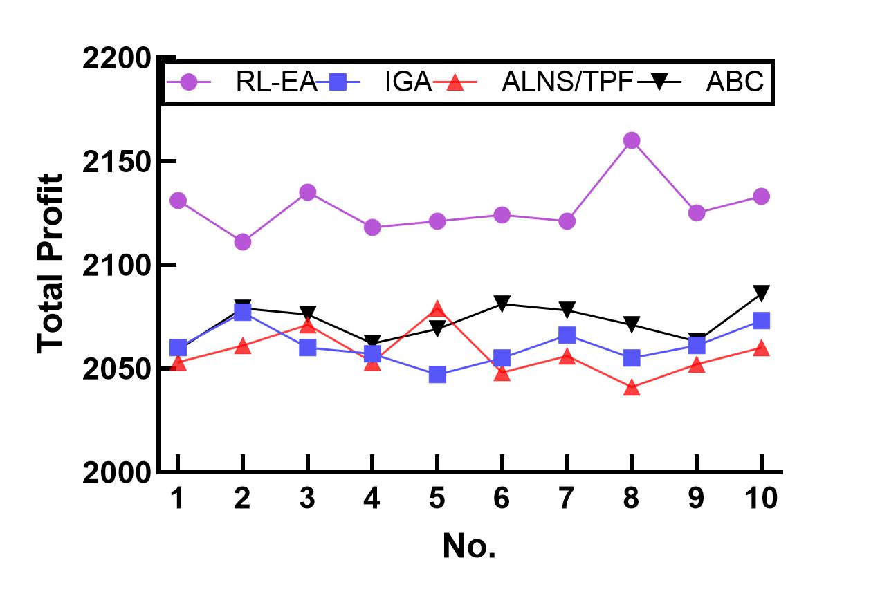
(a) Performance of instance No. 300-4

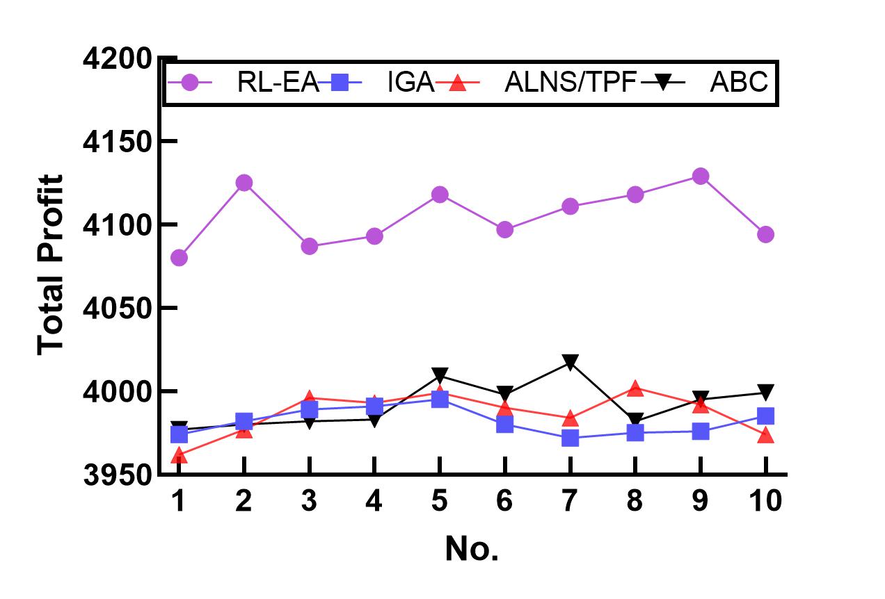
(b) Performance of instance No. 600-4

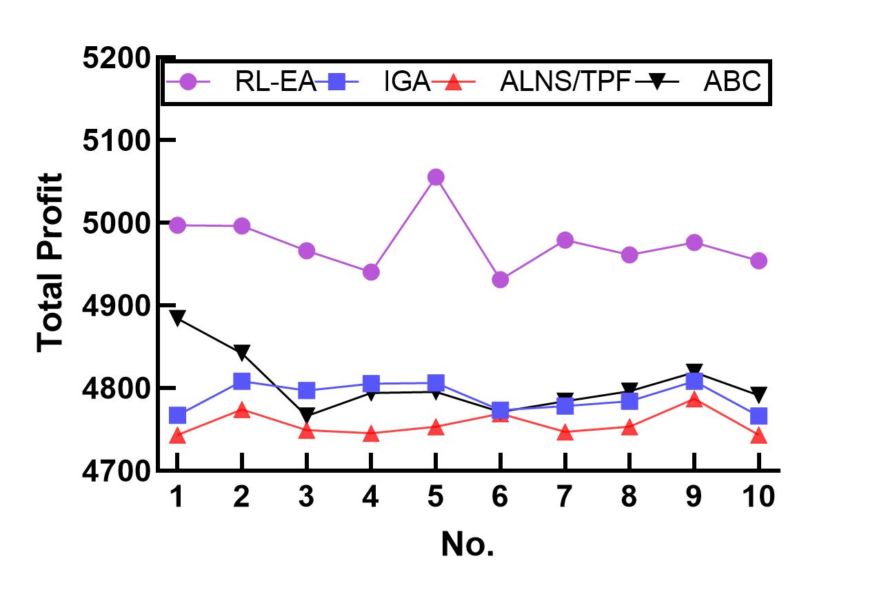
(c) Performance of instance No. 800-4

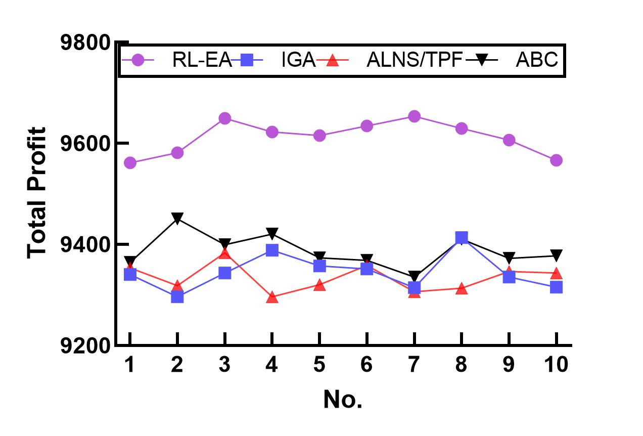
(d) Performance of instance No. 1400-4

Figure 5: Results of 10 Runs of Instances

In addition, we also use the traditional genetic algorithm and an improved genetic algorithm called the GA_ELUMS algorithm to test the problem-solving ability for ultra-large-scale instances, and the results are shown in Table 5.

Table 5: Comparison results with traditional GA and GA_ELUMS

Instance	RL-GA		Traditional GA		GA_ELUMS
	Best	Mean(Std. Dev.)	Best	Mean(Std. Dev.)	Best	Mean(Std. Dev.)
1000-1	8003	7939.33(15.24)	7852	7784.07(22.44)-	7884	7838.47(17.97)-
1000-2	7821	7788.6(16.31)	7732	7677.9(21.43)-	7740	7708.6(17.54)-
1000-3	7907	7882.27(13.95)	7831	7801.53(17.25)-	7857	7831.97(19.77)-
1000-4	8091	8045.57(14.01)	7953	7912.1(20.35)-	7987	7953.37(16.34)-
1100-1	8452	8401.7(17.73)	8357	8271.37(26.34)-	8350	8307(17.78)-
1100-2	8718	8649.27(18.72)	8494	8442.57(24.25)-	8568	8500.63(23.07)-
1100-3	8830	8778.8(18.52)	8660	8615.1(19.81)-	8707	8667(19.2)-
1100-4	8576	8509.63(16.37)	8412	8361.33(24.02)-	8445	8405.77(17.33)-
1200-1	9271	9179.4(26.41)	9048	8961.9(33.16)-	9080	9020.13(25.91)-
1200-2	9039	8958.4(28.03)	8822	8732.57(34.24)-	8846	8790.63(30.02)-
1200-3	9302	9247.5(19.11)	9064	9003.97(28.18)-	9136	9067.43(28.53)-
1200-4	9234	9170.83(16.59)	9027	8950.7(32.27)-	9073	9015.8(23.49)-
1300-1	9566	9491.67(24.62)	9306	9229.23(29.77)-	9368	9304.37(26.95)-
1300-2	9421	9358.4(17.76)	9196	9132.87(28.75)-	9272	9201.13(26.26)-
1300-3	9376	9294.5(17.41)	9143	9030.8(37.1)-	9170	9110.6(26.66)-
1300-4	9389	9309.63(27.44)	9167	9090.6(33.94)-	9210	9147.4(22.58)-
1400-1	9634	9533.1(33.86)	9291	9235.37(34.16)-	9381	9312.7(34.48)-
1400-2	10105	10034.5(28.55)	9790	9724.87(35.96)-	9875	9815.73(29.2)-
1400-3	9793	9699.1(25.56)	9512	9436.17(41.77)-	9591	9513.97(32.25)-
1400-4	9764	9589.5(26.46)	9476	9324.37(45.95)-	9427	9391.4(27.52)-

From Table 5, it can be seen that the RL-GA algorithm has better planning performance compared with the traditional GA algorithm and the GA_ELUMS algorithm [41]. The GA_ELUMS algorithm uses a series of improved strategies containing initialization, crossover, variation, and individual selection, but these strategies are not strong enough to learn and it is difficult to adjust the search strategy by the information obtained from the search. In contrast, the Q-learning method in the RL-GA algorithm dynamically decides on the operations throughout the population evolution process. This learning method can effectively improve the algorithm’s ability to search the problem solution space.

More intuitively, the algorithm results of 300-4, 600-4, 800-4, and 1400-4 running 10 times are shown. The results are shown in Figure 5(a), Figure 5(b), Figure 5(c) and Figure 5(d). As can be seen from the figure, the RL-GA algorithm can maintain good stability while obtaining high profit.

4.2.2 Convergence Analysis

Figures 6(a), 6(b), 6(c) and 6(d) show the convergence speed of different algorithms at 300, 600, 800, and 1400 task scales, respectively. In a small-scale instance, when the number of fitness evaluations reaches 3000, the performance of the algorithm is no longer improved. When the task scale is larger, more search algebras are required for the algorithm to converge. Compared with the compared state-of-the-art algorithms, the RL-GA algorithm has a faster algorithm convergence speed and can exploit continuously.

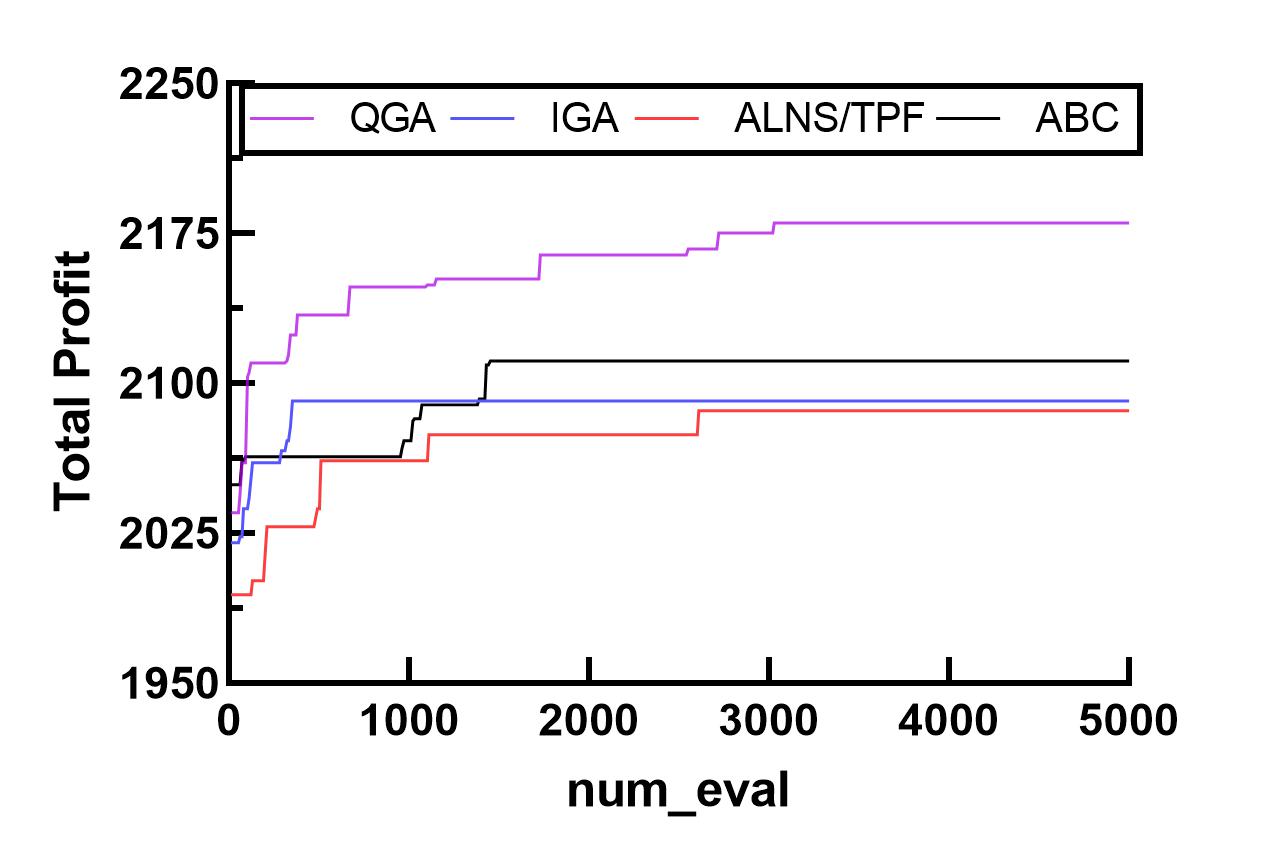
(a) Convergence curves under 300 task scale

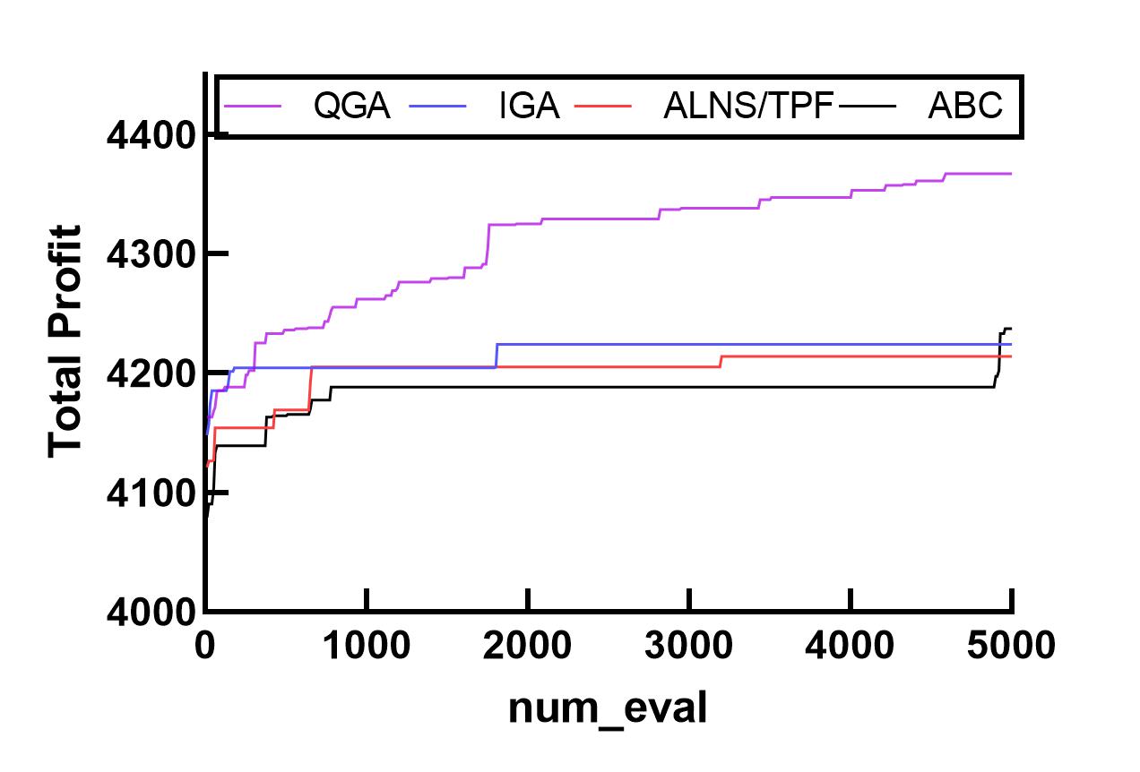
(b) Convergence curves under 600 task scale

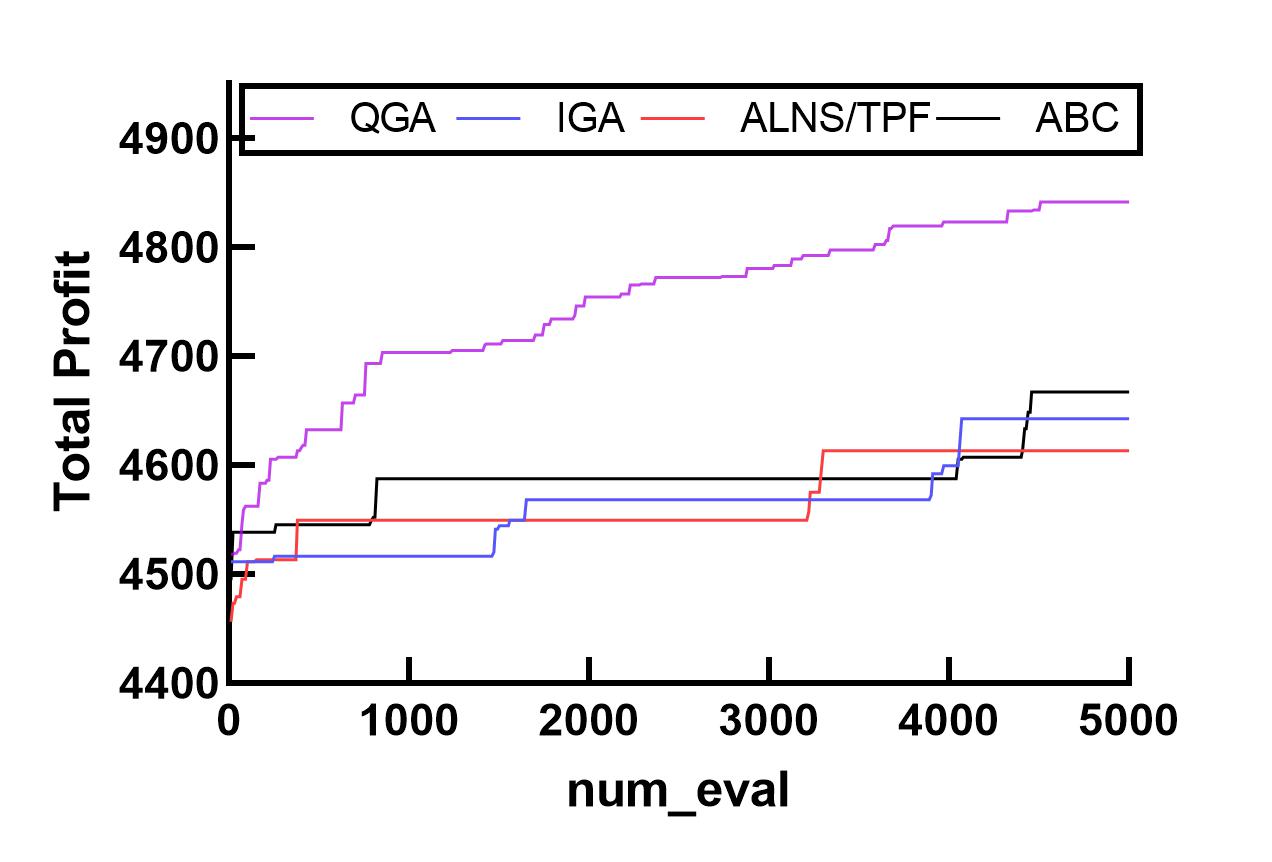
(c) Convergence curves under 800 task scale

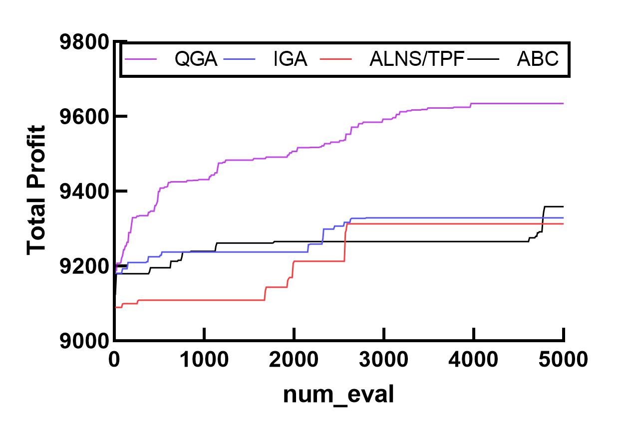
(d) Convergence curves under 1400 task scale

Figure 6: Convergence Curves of Different Scale Instances

4.2.3 CPU Time Analysis

We make statistics on algorithms’ CPU time. The results in Table 6 are the meantime results. It can be seen from the results that the increase in time mainly comes from the increase in problem scale, and the time used for task time window selection increases significantly. When the task scale is small, the running time of the proposed algorithm is not dominant due to the existence of a series of operations of Q value calculation and action selection. When the task scale increases, the task sequence generated by the RL-GA algorithm in the front position has a high possibility of being successfully scheduled. When the time window resource cannot be scheduled, the task time window selection algorithm will not be run to try to schedule. So the computational resources consumed by the reinforcement learning in the algorithm can be ignored. It is not difficult to find that the ABC algorithm takes a lot of time, which is closely related to the complex division of labor within the population and the interaction of bees’ search information. Since the environment of practical problems is often very complex, and the task scale is large, the proposed algorithm is competent for task scheduling.

Table 6: Mean CPU Time(s) for Ultra-large-scale instances

Instance	RL-GA	IGA	ALNS/TPF	ABC
1000-1	2.54	2.53	2.55	6.54
1000-2	2.67	2.73	2.72	6.50
1000-3	2.61	2.57	2.58	6.19
1000-4	2.55	2.68	2.67	6.27
1100-1	2.92	3.02	3.01	7.27
1100-2	2.89	2.99	2.98	7.14
1100-3	2.91	2.92	2.94	6.90
1100-4	2.90	2.90	2.92	7.03
1200-1	3.21	3.28	3.32	8.08
1200-2	3.34	3.35	3.46	8.27
1200-3	3.40	3.64	3.52	8.94
1200-4	3.28	3.35	3.32	8.68
1300-1	3.79	4.03	3.96	9.47
1300-2	3.66	3.77	3.75	9.14
1300-3	3.54	3.65	3.61	9.38
1300-4	3.46	3.59	3.56	8.82
1400-1	4.12	4.19	4.18	10.82
1400-2	4.00	4.10	4.05	10.84
1400-3	4.21	4.26	4.40	10.78
1400-4	4.10	4.34	4.41	11.54

It can be seen from the above experiments that RL-GA achieves better results than other comparison algorithms in terms of profit, stability, convergence speed, and CPU time. From the perspective of problem scale, the RL-GA algorithm has a good performance on large-scale problems, but its time advantage is not obvious in small-scale problems due to its Q-value evaluation and selection mechanism. From the statistical test results of the above experiments, there is a significant difference between the RL-GA algorithm proposed and other comparison algorithms at the level of $p=0.05$ in the majority of instances.

4.2.4 Strategy Comparison Analysis

Afterward, we examine whether the elite individual retention strategy can play a role in the RL-GA algorithm. We select four instances under the task scale of 300, 600, 800, and 1400 to compare the RL-GA algorithm and the RL-GA algorithm (donated as RL-GA/WE) after removing the elite individual retention strategy. The average results of returns are shown in Figure 7(a), Figure 7(b), Figure 7(c), and Figure 7(d), and it can be seen that the elite individual retention strategy makes sense for RL-GA. The RL-GA algorithm that contains an elite individual retention strategy can always achieve higher profit.

In the following, we will use a case study to verify the performance of the RL-GA algorithm in a real project.

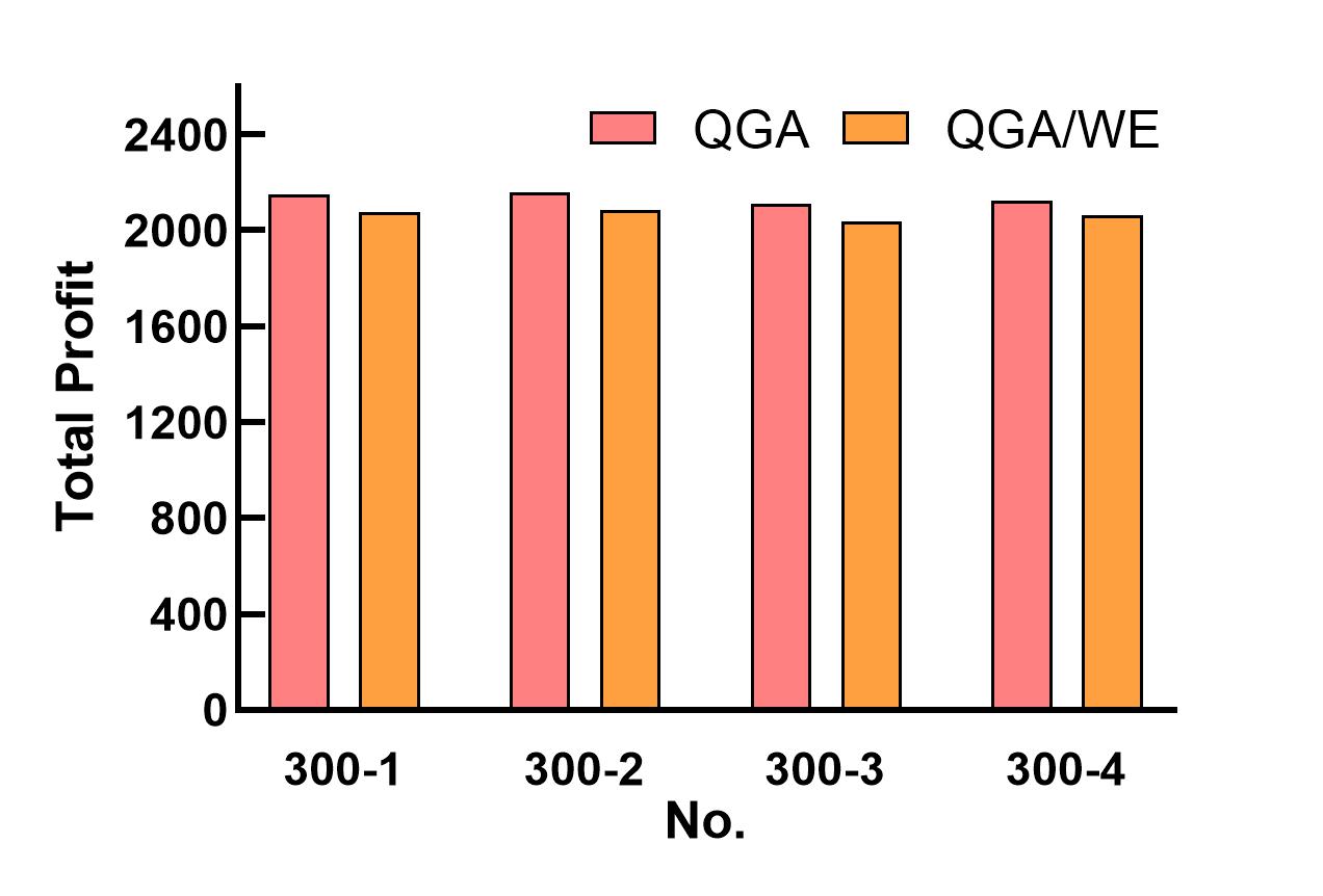
(a) Strategy comparison Results under 300 task scale

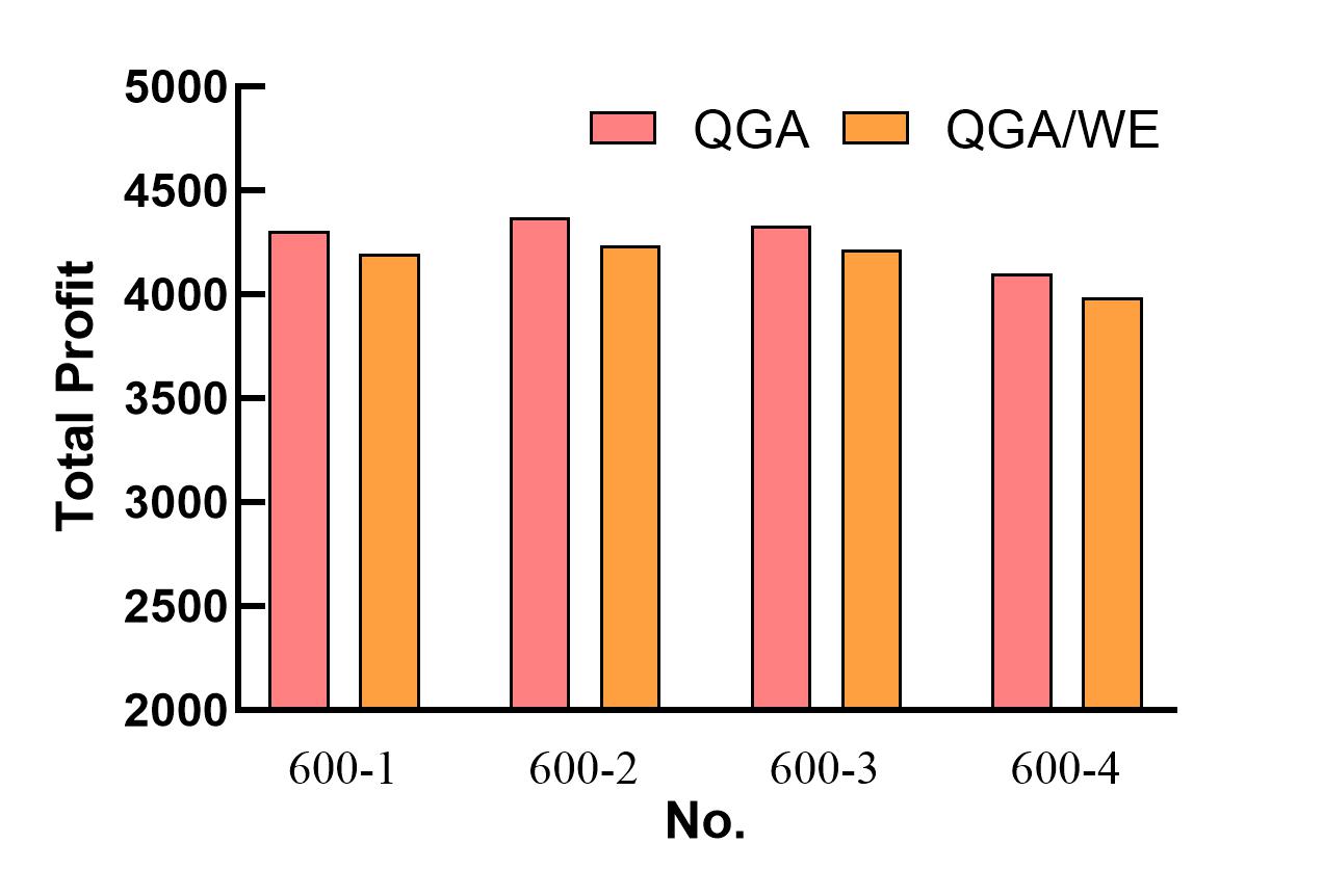
(b) Strategy comparison Results under 600 task scale

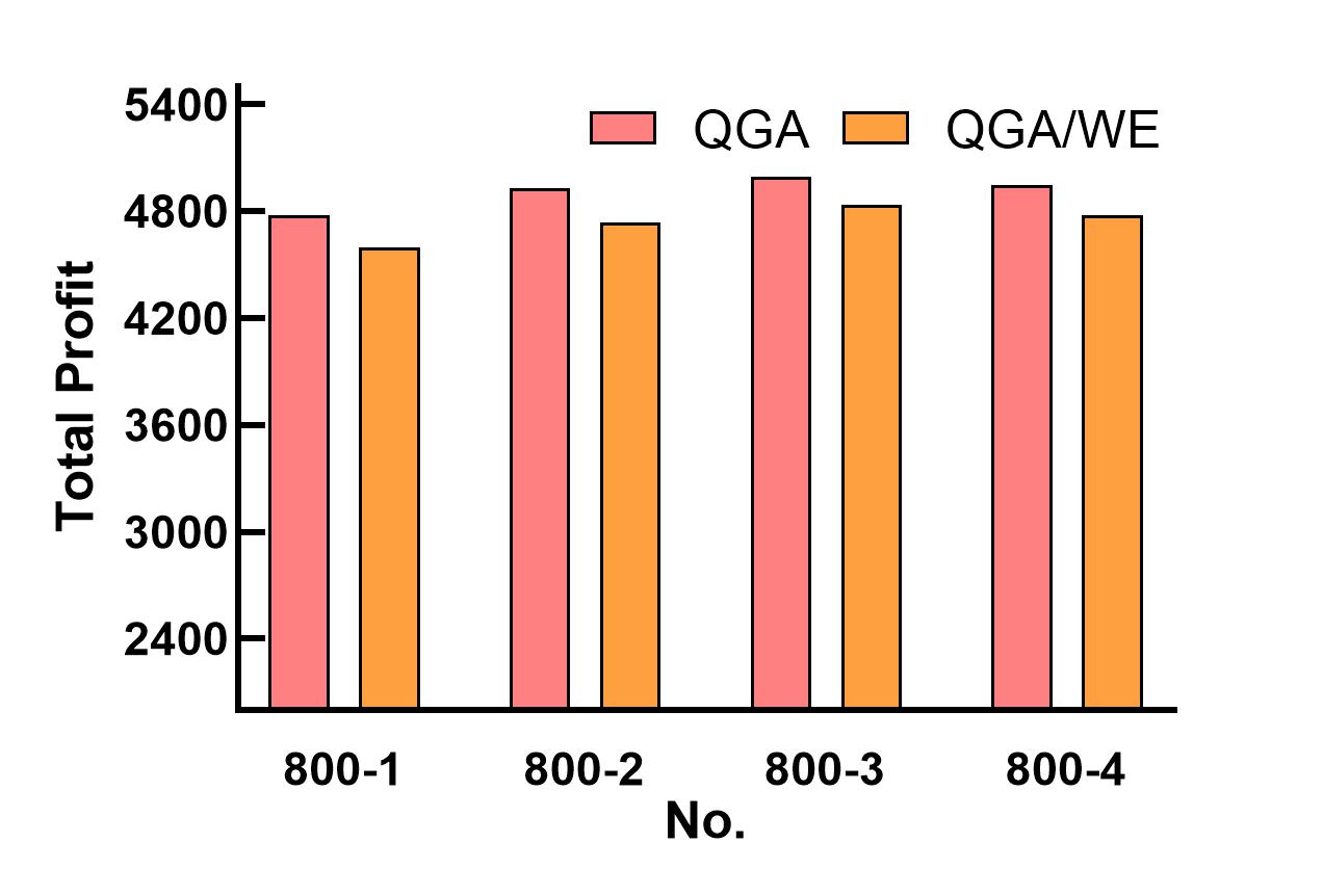
(c) Strategy comparison Results under 800 task scale

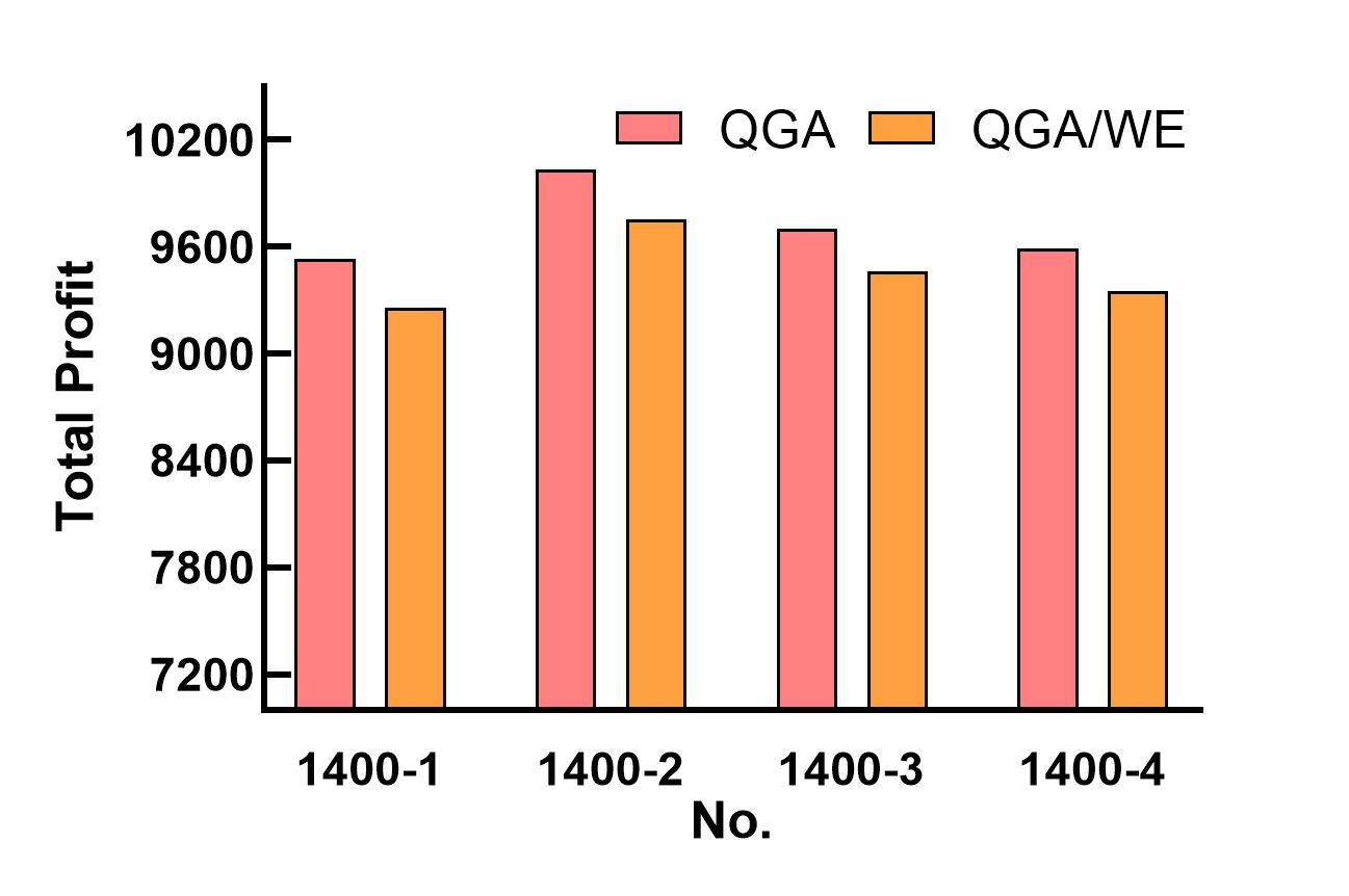
(d) Strategy comparison Results under 1400 task scale

Figure 7: Strategy comparison Results of Different Scale Instances

4.2.5 Case Study

The satellite scheduling system contains a central node and several user nodes, where the user nodes are responsible for submitting applications and the central node deploys mission planning software for generating execution plans. After the user applies, the central node will pre-process it based on a series of information such as location, satellite orbit, and other requirements. The pre-processing will remove duplicate tasks, merge similar tasks, and split tasks that cannot be detected at once. Preprocessing also calculates the visible time window of each task. Once the preprocessing is complete, the input data needed for scheduling is obtained, including satellites, tasks, and time windows.

The satellite scheduling system tends to use a week as a scheduling cycle. We use the RL-GA algorithm proposed in this paper to plan each day’s tasks separately, obtain the execution plan for a single day, and then accumulate to get the execution plan for the whole week. Here, we let the system plan 1000 tasks per day, and the scheduling results are shown in Figure 8(a). The task completion rate is also a factor considered in practical applications, and the successful task execution rate for each day is given in Figure 8(b).

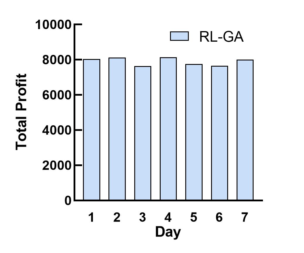
(a) Detection Profit

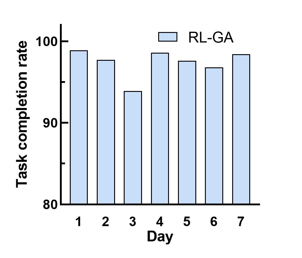
(b) Task Completion Rate

Figure 8: Scheduling Results of the Satellite Scheduling System

As shown in Figure 8, the satellite scheduling system obtains a steady daily profit and less than 10% of the tasks cannot be completed. After generating the plan, the satellite scheduling system will check the correctness of the generated solution and pass the test by generating satellite commands to the satellites that need to execute tasks through ground stations. The satellite will execute each task according to the start and end time set in the plan and transmit the data obtained to the ground station through data downlink. The data is processed accordingly and distributed to the user who submitted the request. The processing flow of the satellite scheduling system is shown in Figure 9.

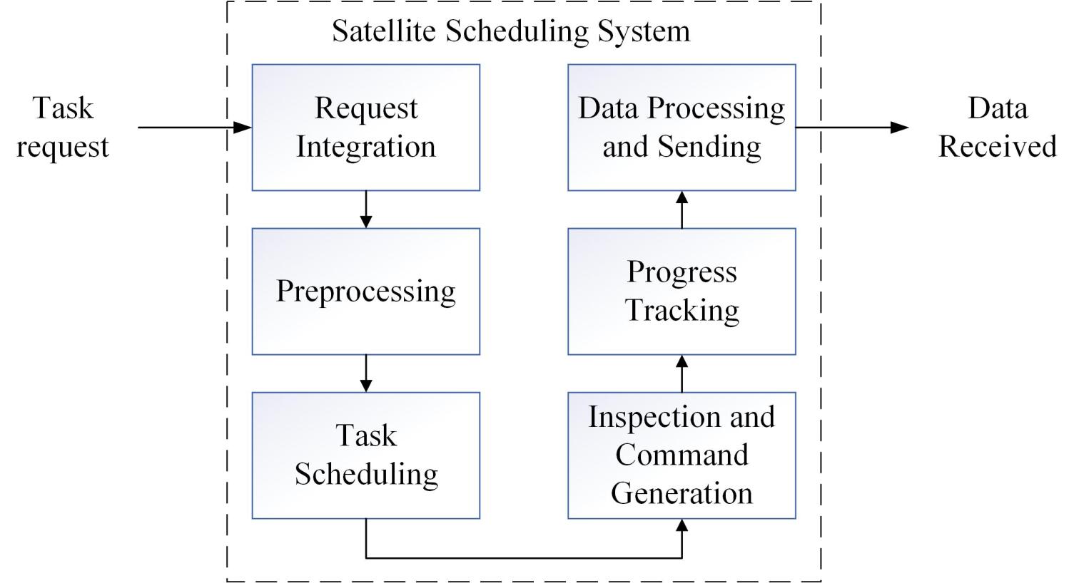
Figure 9: Processing Flow of the Satellite Scheduling System

From the above results, we can see that our proposed algorithm can solve the EDSSP problem well and verify the effectiveness of the algorithm from several aspects. the RL-GA algorithm not only can get high-quality solutions but also can solve the problem quickly. Large-scale instances and ultra-large-scale instances further prove the ability of the RL-GA algorithm to solve practical problems. The results of real cases verify that the algorithm can maintain good planning performance throughout the system’s multi-day operation and is available for long-term use.

5 Conclusion

In this paper, we propose a reinforcement learning-based genetic algorithm to solve the EDSSP problem. The genetic algorithm based on reinforcement learning uses a new combination method of Q-learning and GA algorithm, which allows the algorithm to select operators autonomously through adaptive learning, giving the algorithm a strong ability to adapt to different scenarios. The agent can choose effective actions based on the interaction with the environment during the search process to improve search performance. The population search process in the evolutionary algorithm is guided by reinforcement learning, which allows each individual to select an appropriate strategy according to the reward and Q value. We construct a $<$state, action$>$ combination method according to the search performance and update the corresponding value after each evolution is completed. The elite individual retention strategy also used in the algorithm can improve search performance. It can be seen from the experiments that our proposed algorithm has obvious advantages in solving the EDSSP problem.

LA-GA effectively solves the EDSSP problem and enables the satellite scheduling system to obtain a high-quality mission execution plan in a short time. The proposed algorithm can effectively cope with the increase in the number of satellites and tasks. In addition, the problem-solving idea is also applicable to other combinatorial optimization problems with order dependence.

In future research, we will try to reduce the computational cost of the Q-value evaluation mechanism to further accelerate the search speed without affecting the performance of the algorithm. Other learning methods will also be considered, such as transfer learning, deep learning, and others. In addition, we will consider applying learning-based approaches to the online scheduling problem. This type of scheduling problem has higher requirements for the algorithm.

6 Declaration of Competing Interest

The authors declare that they have no known competing financial interests or personal relationships that could have appeared to influence the work reported in this paper.

7 Acknowledgements

This work was supported by the National Natural Science Foundation of China (71901213, 61773120, 72001212), the Special Projects in Key Fields of Universities in Guangdong (2021ZDZX1019), and the Hunan Provincial Innovation Foundation For Postgraduate (CX20200585).

Thanks to the editor and reviewers for their valuable comments. We also thank Dr. Luona Wei and Dr. Yongming He for their guidance on the method.

Luona Wei and Yanjie Song contribute equally to this article.

References

- [1] Lin, Wei-Cheng, et al. ”Daily imaging scheduling of an earth observation satellite.” IEEE Transactions on Systems, Man, and Cybernetics-Part A: Systems and Humans 35.2 (2005): 213-223.
- [2] LI Yaodong, and ZHANG Jing. ”Research on Mission Scheduling of Electronic Reconnaissance Satellites Based on Multi-area.” DEStech Transactions on Engineering and Technology Research iceea (2016).
- [3] Li, Changchun, and Zhu Jianghan. ”Research on the Method of Electronic Reconnaissance Satellites Mission Planning for Continuous Reconnaissance of Moving Target.” Journal of the Academy of Equipment Command & Technology (2011).
- [4] Wang, Xinwei, et al. ”Agile earth observation satellite scheduling over 20 years: Formulations, methods, and future directions.” IEEE Systems Journal 15.3 (2020): 3881-3892.
- [5] Xhafa, Fatos, and Andrew WH Ip. ”Optimisation problems and resolution methods in satellite scheduling and space-craft operation: a survey.” Enterprise Information Systems 15.8 (2021): 1022-1045.
- [6] Barbulescu, Laura, et al. ”Scheduling space–ground communications for the air force satellite control network.” Journal of Scheduling 7.1 (2004): 7-34.
- [7] Berger, Jean, Nassirou Lo, and Mohamed Barkaoui. ”QUEST–A new quadratic decision model for the multi-satellite scheduling problem.” Computers & Operations Research 115 (2020): 104822.
- [8] Cho, Doo-Hyun, et al. ”Optimization-based scheduling method for agile earth-observing satellite constellation.” Journal of Aerospace Information Systems 15.11 (2018): 611-626.
- [9] Niu, Xiaonan, Tang Hong, and Wu Lixin. ”Satellite scheduling of large areal tasks for rapid response to natural disaster using a multi-objective genetic algorithm.” International journal of disaster risk reduction 28 (2018): 813-825.
- [10] Chen, Xiaoyu, et al. ”A mixed integer linear programming model for multi-satellite scheduling.” European Journal of Operational Research 275.2 (2019): 694-707.
- [11] Zheng, Zixuan, Jian Guo, and Eberhard Gill. ”Swarm satellite mission scheduling & planning using hybrid dynamic mutation genetic algorithm.” Acta Astronautica 137 (2017): 243-253.
- [12] Li, Zhiliang, and Xiaojiang Li. ”A multi-objective binary-encoding differential evolution algorithm for proactive scheduling of agile earth observation satellites.” Advances in Space Research 63.10 (2019): 3258-3269.
- [13] Chen, Xiang-guo, and Wu Xiao-yue. ”ACO algorithm of satellite data transmission scheduling based on solution construction graph.” Syst. Eng. Electron. 32 (2010): 592-597.
- [14] Xiang, Shang, et al. ”Knowledge-based memetic algorithm for joint task planning of multi-platform earth observation system.” Computers & Industrial Engineering 160 (2021): 107559.
- [15] Xhafa, Fatos, et al. ”Evaluation of struggle strategy in genetic algorithms for ground stations scheduling problem.” Journal of computer and system sciences 79.7 (2013): 1086-1100.
- [16] Barbulescu, Laura, et al. ”Understanding algorithm performance on an oversubscribed scheduling application.” Journal of Artificial Intelligence Research 27 (2006): 577-615.
- [17] Zhibo, E., et al. ”Multi-satellites imaging scheduling using individual reconfiguration based integer coding genetic algorithm.” Acta Astronautica 178 (2021): 645-657.
- [18] Zhang, Jiawei, and Lining Xing. ”An improved genetic algorithm for the integrated satellite imaging and data transmission scheduling problem.” Computers & Operations Research 139 (2022): 105626.
- [19] Song, Yan-Jie, et al. ”Learning-guided nondominated sorting genetic algorithm II for multi-objective satellite range scheduling problem.” Swarm and Evolutionary Computation 49 (2019): 194-205.
- [20] Du, Yonghao, et al. ”MOEA based memetic algorithms for multi-objective satellite range scheduling problem.” Swarm and Evolutionary Computation 50 (2019): 100576.
- [21] Xhafa, Fatos, et al. ”Genetic algorithms for satellite scheduling problems.” Mobile Information Systems 8.4 (2012): 351-377.
- [22] Wei, Luona, et al. ”Deep reinforcement learning and parameter transfer based approach for the multi-objective agile earth observation satellite scheduling problem.” Applied Soft Computing 110 (2021): 107607.
- [23] Chen, Ming, et al. ”Deep reinforcement learning for agile satellite scheduling problem.” 2019 IEEE Symposium Series on Computational Intelligence (SSCI). IEEE, 2019.
- [24] Hsieh, Yi-Zeng, and Mu-Chun Su. ”A Q-learning-based swarm optimization algorithm for economic dispatch problem.” Neural Computing and Applications 27.8 (2016): 2333-2350.
- [25] Li, Zhihui, et al. ”Differential evolution based on reinforcement learning with fitness ranking for solving multimodal multi-objective problems.” Swarm and Evolutionary Computation 49 (2019): 234-244.
- [26] Tian, Ye, et al. ”Deep Reinforcement Learning Based Adaptive Operator Selection for Evolutionary Multi-Objective Optimization.” IEEE Transactions on Emerging Topics in Computational Intelligence (2022).
- [27] Rodríguez-Esparza, E., Masegosa, A. D., Oliva, D., & Onieva, E. (2022). A new Hyper-heuristic based on Adaptive Simulated Annealing and Reinforcement Learning for the Capacitated Electric Vehicle Routing Problem. arXiv preprint arXiv:2206.03185.
- [28] Zhang X, Xia S, Li X, et al. Multi-objective particle swarm optimization with multi-mode collaboration based on reinforcement learning for path planning of unmanned air vehicles[J]. Knowledge-Based Systems, 2022: 109075.
- [29] Du, Y., Li, J. Q., Chen, X. L., Duan, P. Y., & Pan, Q. K. (2022). Knowledge-Based Reinforcement Learning and Estimation of Distribution Algorithm for Flexible Job Shop Scheduling Problem. IEEE Transactions on Emerging Topics in Computational Intelligence.
- [30] He, Y., Xing, L., Chen, Y., Pedrycz, W., Wang, L., & Wu, G. (2020). A generic Markov decision process model and reinforcement learning method for scheduling agile earth observation satellites. IEEE Transactions on Systems, Man, and Cybernetics: Systems.
- [31] Wei, L., Xing, L., Wan, Q., Song, Y., & Chen, Y. (2021). A multi-objective memetic approach for time-dependent agile earth observation satellite scheduling problem. Computers & Industrial Engineering, 159, 107530.
- [32] Peng, G., Dewil, R., Verbeeck, C., Gunawan, A., Xing, L., & Vansteenwegen, P. (2019). Agile earth observation satellite scheduling: An orienteering problem with time-dependent profits and travel times. Computers & Operations Research, 111, 84-98.
- [33] Barbulescu, Laura, et al. ”Scheduling space–ground communications for the air force satellite control network.” Journal of Scheduling 7.1 (2004): 7-34.
- [34] Vallada, Eva, and Rubén Ruiz. ”A genetic algorithm for the unrelated parallel machine scheduling problem with sequence dependent setup times.” European Journal of Operational Research 211.3 (2011): 612-622.
- [35] Sutton, Richard S., and Andrew G. Barto. Reinforcement learning: An introduction. MIT Press, 2018.
- [36] Kumar, Aviral, et al. ”Conservative q-learning for offline reinforcement learning.” Advances in Neural Information Processing Systems 33 (2020): 1179-1191.
- [37] Watkins, Christopher JCH, and Peter Dayan. ”Q-learning.” Machine learning 8.3 (1992): 279-292.
- [38] Song, Bingyu, et al. ”A hybrid genetic algorithm for satellite image downlink scheduling problem.” Discrete Dynamics in Nature and Society 2018 (2018).
- [39] He, Lei, et al. ”An improved adaptive large neighborhood search algorithm for multiple agile satellites scheduling.” Computers & Operations Research 100 (2018): 12-25.
- [40] Pan, Quan-Ke, et al. ”A discrete artificial bee colony algorithm for the lot-streaming flow shop scheduling problem.” Information sciences 181.12 (2011): 2455-2468.
- [41] Zhang, J., & Xing, L. (2022). An improved genetic algorithm for the integrated satellite imaging and data transmission scheduling problem. Computers & Operations Research, 139, 105626.