Novel Sample Stages for Detecting Magnetic Feedback Due to
Superconducting Transition Based on the Mirror Image Method

Abstract

In traditional detection of the magnetic signalYusa et al. (2021); Tuzlukov (2001); Pastore and Scheirer (1974) in the experiment, complicated electronic devices are usually set up to explore the feedback from the superconducting transition due to the external magnetic field. This kind of direct detection will be more time-consuming, especially in experiments with strict requirements like low temperature and high vacuum. To make the signal detection more convenient to realize, we design a novel sample stage with functions of both placement and acceptance of the magnetic field based on the mirror image methodXifre-Perez et al. (2013); Yakushev (2013). This device consists of two parts, drive coils and receiver coils. The drive coils apply the initial magnetic field to the superconducting material while the receiver coils are used to collect the magnetic signal feedback. With only the power supply and a signal amplifier needed to be connected to the coils, our device makes it more convenient to finish magnetic signal detection. Another highlight of our design is using first-principles numerical simulation to help accurately determine the size and parameters of the device. With these calculated parameters, we build a 3D model of the device using the software SOLIDWORKS.

I Introduction

In experiments to explore the magnetic properties of superconducting materials, ultra-high vacuum and low temperature are often necessary conditions. The traditional detectionZhao et al. (2021); Tian et al. (2022) of magnetic signals under such conditions will always require complicated electronic devices including an initial signal generator, a traditional sample stage, a receiver and a signal filter, as shown in the Fig. 2(a). Both applying and receiving the magnetic signal will be usually time-consuming with such a series of devices. To make the detection more convenient, we modified the sample stage to be equipped with drive coils and receiver coils. Therefore, we could simplify the detection process with this novel sample stage as Fig. 2(b) shows. Only two wires are needed to connect our designed device with the outside power supply and the signal amplifier Brkovic et al. (1994).

The sample material to be tested is placed on the novel sample stage in Fig.2(d) and sent into the chamber. Once the sample stage is in place, the interior of the chamber must be isolated from the outside world. Therefore, a well-designed stage with an accurate size is important to ensure that the feedback magnetic field is large enough to be measured. To find the appropriate parameters of our device model, we refer to the mirror image methodEmig (2008); Xifre-Perez et al. (2013). In addition, we apply the Messner EffectEssén and Fiolhais (2012) theory to numerically simulate the magnetic signal feedback due to the superconducting transition. The highlight of our simulation is that we could separate initial and feedback magnetic signals so it will be easier for conducting the signal-filtering process in the experiment.

We show the 3D model diagram of the device using the software SOLIDWORKS. Moreover, to reduce the error caused by the boundary effect of magnetic fieldIverson and Kuhl (1995); Naitou et al. (1979), we analyze in FIG. 6 to discuss the critical size of the sample stage, which is large enough that the boundary effect can be ignored.

II NUMERICAL SIMULATION MODEL

In order to simultaneously apply the magnetic field and detect the magnetic field feedback, we place the drive coils and receiver coils above the sample materials. The simulation of the initial magnetic field applied by the drive coils can be realized with the Biot-Savart lawCharitat and Graner (2003); Oliveira and Miranda (2001). The feedback magnetic signal due to superconducting transition is numerically simulated referring to the mirror image method.

II.1 Drive Coils to Apply the Magnetic Field

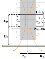
Figure 1: The drive coils are connected to the power supply and will apply the initial magnetic field to the sample material. The inset shows the definition of some important parameters in equation (1).

Figure 2: (a) The traditional detection process of the magnetic signal. (b) The novel detection process of magnetic signal with the novel sample stage. (c) The traditional sample stage for holding sample materials. (d) The novel sample stage with drive coils and receiver coils connected with the outside power supply and the signal amplifier.

In FIG.1, $\rm L_{D}$ is the length of drive coils while $\rm H_{0}$ stands for the distance between the bottom of drive coils and sample materials. $\rm r_{C}$ and $\rm R_{S}$ separately represent the radius of drive coils and that of sample materials. The drive coils are connected to the external AC power supply. The current in the coils satisfies $\rm I=I_{0}sin(\omega t)$, where $\rm\omega=2\pi f$ is the angular frequency. By applying the Biot-Savart law, we obtain the magnitude of the magnetic field $\rm B(h)$ generated by each coil at a point on its axis at a distance $\rm h$.

$$\rm\boldsymbol{B}(h)=\frac{\mu_{0}}{4\pi}\oint\frac{Id\overrightarrow{\boldsymbol{r_{i}}}\times(\overrightarrow{\boldsymbol{r}}-\overrightarrow{\boldsymbol{r_{i}}})}{|\overrightarrow{\boldsymbol{r}}-\overrightarrow{\boldsymbol{r_{i}}}|^{3}}\\ =\frac{\mu_{0}I}{4\pi}\sum_{i=0}^{N_{\theta}}\frac{r_{C}d\theta\overrightarrow{\boldsymbol{e_{i}}}\times(-\overrightarrow{\boldsymbol{r_{i}}})}{(h^{2}+r_{C}^{2})^{\frac{3}{2}}}$$ (1)

The equation (1) represents for the discretization of Biot-Savart lawAlbani and Bernardi (1974); Árnason (1999); Bossavit (2005), and the circumference angle $\rm\theta$ is discretized into $\rm N_{\theta}$ parts. We sum the magnetic field strengths $\rm B_{D}$ generated by $\rm N_{D}$ drive coils on the axis to obtain the magnetic field distribution on the axis of the drive coils.

$$\rm\boldsymbol{B}_{D}(h_{0},N_{D})=\sum_{i=0}^{N_{D}-1}\boldsymbol{B}(h_{0}+i\Delta L)$$ (2)

$\rm h_{0}$ refers to the distance between the bottom of the drive coil and the point on the axis. For example, if we consider the distance from the center of the sample then $\rm h_{0}=H_{0}$ (See FIG. 1). The distance between adjacent coils $\rm\Delta L$ in equation(2) is determined by $\rm L_{D}/N_{D}$.

II.2 Receiver Coils and the Mirror Image Method

The magnetic field generated by the drive coils will pass the sample material. With a temperature lower than the superconducting critical temperature, a surface current will form on the sample according to the Meissner effectBardeen (1955); Schafroth (1958), and the magnetic field generated by the surface current will change the magnetic field in the space. We use mirror coils to simulate the magnetic field feedback due to the surface current.

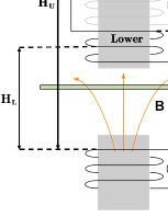
Figure 3: The receiver coils are connected to the amplifier to amplify the feedback magnetic signal due to the superconducting transition. The mirror coils are the mirror image of the drive coils relative to the sample stage.

In FIG. 3, $\rm H_{U}$ stands for the distance between the middle of upper receiver coils and the top of mirror coils, while $\rm H_{L}$ is the distance between the middle of lower receiver coils and mirror coils top. $\rm L_{R}$ and $\rm L_{M}$ separately represent the length of lower/upper receiver coils and mirror coils

We divide the receiver coils into two parts, the upper and the lower coils. Both these two parts have the same length $\rm L_{R}$ and the same number of coils $\rm N_{R}$. The drive coils are set in the middle of these two parts so as to eliminate the influence of the magnetic field generated in the receiver coils by the drive coils because the produced electromotive force in the upper and lower receiver coils will be equal and reversed. In order to simplify the calculation, We assume that the magnetic field generated by the mirror coils inside the receiver coils is constant and can be replaced by the magnetic field generated by the mirror coils in the middle of the receiver coils.

Based on the Faraday electromagnetic induction lawGiuliani (2008); Galili et al. (2006), we obtain the electromotive force difference $\rm\Delta U$ generated by the mirror coils at the receiver coils in the equation (3).

$$\rm\Delta U \rm=|U_{U}-U_{L}|$$ (3)

$$\rm=|-N_{R}\pi r_{C}^{2}\frac{dB_{D}(H_{L},N_{D})-dB_{D}(H_{U},N_{D})}{dt}|$$

$$\rm=N_{R}f\pi r_{C}^{2}\frac{\mu_{0}I_{rms}}{2}|\sum_{i=0}^{N_{D}-1}\Big{\{}\sum_{j=0}^{N_{\theta}}\frac{r_{C}d\theta[\overrightarrow{\boldsymbol{e_{j}}}\times(-\overrightarrow{\boldsymbol{r_{j}}})]_{z}}{[(H_{U}+\frac{iL_{D}}{N_{D}})^{2}+r_{C}^{2}]^{\frac{3}{2}}}-\sum_{j=0}^{N_{\theta}}\frac{r_{C}d\theta[\overrightarrow{\boldsymbol{e_{j}}}\times(-\overrightarrow{\boldsymbol{r_{j}}})]_{z}}{[(H_{L}+\frac{iL_{D}}{N_{D}})^{2}+r_{C}^{2}]^{\frac{3}{2}}}\Big{\}}|$$

The potential difference shown in equation (3) can be amplified by the amplifierUranga et al. (2004); GUIDE for subsequent analysis. The existing instrument can measure the potential difference greater than 100nV. That is to say, as long as the measured potential difference is greater than 100nV, it can satisfy the needs of the experiment.

II.3 Determination of Parameters in the Model

In equation (3), there are many parameters set to be constant, such as $\rm N_{R}$, $\rm N_{D}$, $\rm r_{C}$ and $\rm\Delta L$ in this paper. This requires us to fix these parameters when designing the model. To ensure that the voltage difference received by the receiver coils $\rm\Delta U$ during the experiment is large enough, we first decide some parameters according to the size of other experimental devices. For example, the length $\rm L_{D}$ and radius $\rm r_{C}$ of the drive coils should match the sample stage’s size. Therefore, we select some appropriate values for parameters in TABLE 1.

Table 1: Other parameters except $\rm N_{R}$ and $\rm N_{D}$, which are referred to the specifications and sizes of the specific experimental equipment. $\rm I_{rms}$ is the effective value of the alternating current in the drive coils.

$\rm f\ (kHz)$	$\rm r_{C}$ (mm)	$\rm I_{rms}\ (\mu A)$	$\rm H_{L}$ (mm)	$\rm H_{U}$ (mm)	$\rm L_{D}\ (mm)$	$\rm N_{\theta}$
100	2	500	17.5	30.5	8	100

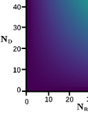
Figure 4: The voltage difference $\rm\Delta U$ is a function of $\rm N_{D}$ and $\rm N_{R}$. $\rm\Delta U$ will exceed 600nV when $\rm N_{R}>50$, $\rm N_{D}>50$.

However, some parameters like the number of coils are flexible and will also affect the detection results. To find the appropriate $\rm N_{D}$ and $\rm N_{R}$ to maximize $\rm\Delta U$, we use the equation (3) to calculate the potential difference as a function of $\rm N_{D}$ and $\rm N_{R}$.

FIG 4 shows us the results of the numerical calculation. It can be seen that the calculated voltage difference increases with the increasing $\rm N_{D}$ and $\rm N_{R}$. However, the number of coil turns should not be too large, if not so the distance between the coils will be would be smaller than the size of the coil itself, which is impossible. We can take $\rm N_{D}$=40, $\rm N_{R}$=30 so the corresponding $\rm\Delta U$ is 314.06nV. It is already greater than the detectable 100nV, so this turns ratio is acceptable.

II.4 3D Modeling of the Device

We can use SOLIDWORKS to draw the 3D modelSchilling and Shih (2019); Akin (2010) diagram to have an intuitive understanding of the model. The scale of the drawing is not drawn according to the real scale, which is for the convenience of display.

From the main view in FIG 5(a), we can see that the entire model is mainly composed of two parts: a movable cylindrical barrel for loading coils and a sample stage for placing samples. The cylindrical barrel consists of three layers, the middle layer is used to place the drive coils, the upper and lower layers are used to place the receiver coils, and each layer has holes to connect with the external driving circuit or receiving circuit. Just below the cylindrical barrel is the place to hold the sample, and the distance $\rm H_{0}$ from the sample to the bottom of the cylindrical barrel can be changed as required.

III The Error Analysis

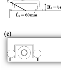
Figure 5: The 3D model is not showed in the real scale for the convenience of display. (a) The front view of the model. A is the compartment where the receiver coils are placed, B is the hole used for connecting the external power supply, C is the compartment where the drive coils are placed and D is the sample stage holding the sample materials. (b) The left view. (c) The top view. (d) The view of the whole model.

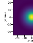
Figure 6: (a) Convergence of magnetic flux $\rm\Phi$ in the sample material with $\rm H_{0}$=8mm, 10mm and 12mm. (b) The initial magnetic field B is applied in the sample plane with height $\rm H_{0}$=10mm.

Usually, further experimental validation could be a good way to prove the reliability of our model design. However, we would like to suggest it as a topic for further research due to a number of complications in experimental detection. Other alternative ways are applied to improve the reliability in this paper. We maximize the fault toleranceAvizienis and Kelly (1984) and analyze the boundary effect to reduce possible errors in our model design. This kind of error analysisBertoni et al. (2003) will also help improve our design so that it can be well-applied to the magnetic signal detection experiments.

III.1 The Fault Tolerance Maximization

When a device is applied to the experimental detection, many parameters will not be able to be revised. Therefore, we should always improve our design to maximize fault tolerance. For example, Fig. 6(a) shows that the magnetic flux $\rm\Phi$ will converge with different values of $\rm R_{S}$ for different $\rm H_{0}$. To maximize the fault tolerance, we should choose the maximum $\rm R_{S}$=30mm to ensure $\rm\Phi$ will converge for different $\rm H_{0}$.

III.2 The Boundary effect

An important prerequisite for the mirror image method is that we can ignore the boundary effect of the samplePan et al. (2020); Shou et al. (2010); Evans et al. (2005); Yu and Girshick (1991). Therefore, we need to estimate the critical length of the stage to ensure that the magnetic field outside the sample stage will be negligible. In FIG 6(b), the magnetic field will decrease to 0 when the position is far from the center of the sample stage, which means that the magnetic field will be negligible compared with the central value when the sample size is larger than 30mm. In fact, there are other numerical simulation methods(details in Appendix B), but they all need to consider the boundary effects of electromagnetic fields.

IV Conclusion

To make the detection of the magnetic signal due to the superconducting transition more convenient, we design a novel sample stage based on the mirror image method. This design adds the drive coils and receiver coils to the traditional sample stage, which reduces many electronic devices and simplifies the detection process. The numerical simulation skills are applied to find the most suitable size parameters for the sample stage. Moreover, we build a 3D model diagram to help understand the 3D structure of our device. We further explore the possible reasons for design errors and try to find a stage size which is large enough to eliminate the boundary effect.

ACKNOWLEDGMENTS

We wish to acknowledge the support of Professor Jing Shi from Wuhan University, China, who encourages us to finish and perfect this project. We also wish to acknowledge the guidance of Professor Yuanbo Zhang, Master Zhiwei Huang and Master Hengsheng Luo from Fudan University, China, providing the experimental environment and gave some important suggestions.

AUTHOR DECLARATIONS

Conflict of Interest

The authors declare no conflicts of interest.

Author Contributions

Ziyan Li is the major contributor and Mengbo Guo is the minor contributor.

DATA AVAILABILITY STATEMENT

The data that support the findings of this study are available within the article [and its supplementary material].

Appendix A Meissner Effect and London Equation

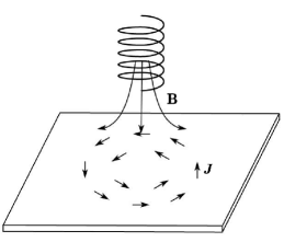
Figure 7: The surface current generated by the magnetic field applied to the superconducting sample materials.

The Meissner effect refers to the phenomenonAnderson and Matthias (1964) that the magnetic field will maintain zero inside the superconducting materials. The London equationKaloper and Lawrence (2017) is a relatively classic and simple explanation model to explain this phenomenon.

This model assumes that electrons in the superconducting state can be divided into two types: electrons in the normal state and electrons in the superconducting state. The surface current density of the material can be related to the corresponding magnetic vector potential:

$$\rm\boldsymbol{J}=-\frac{n_{s}e^{2}}{m_{e}}\boldsymbol{A}$$ (4)

Take the curl for quantities on both sides and refer to Maxwell’s equationLax and Nelson (1976); Assous et al. (1993). Then we can get the relation between current density and magnetic field:

$$\rm\nabla\times\boldsymbol{J}=-\frac{n_{s}e^{2}}{m_{e}}\boldsymbol{B}$$ (5)

$$\rm\nabla\times\boldsymbol{B}=\mu_{0}\boldsymbol{J}$$ (6)

Combining all the above formulas to obtain the magnetic field:

$$\rm\boldsymbol{B}(x)=\boldsymbol{B_{0}}exp(-\frac{x}{\lambda})$$ (7)

Equation (7) shows that the magnetic field decreases exponentially, indicating that the magnetic field cannot penetrate the surface of the sample. As shown in FIG. 7, the surface currentGurevich and Laiho (1993); Gurevich et al. (1992) can be used to calculate the magnetic field feedback generated by the sample. This approach is essentially consistent with the mirror method.

Appendix B Numerical Simulation of Annular Current

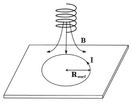
Figure 8: The ring current is used to be in place of the surface current. $\rm R_{surf}$ is the radius of the ring current.

This is also a method similar to using surface currents to simulate feedback magnetic fields, but unlike Appendix A, this method replaces the surface currents with a loop of toroidal currents. The feedback of the superconducting material can be calculated if we know about the value of the current. The method of confirming the magnitude of the current is making the sum of the magnetic fluxes generated by the annular current inside it equal to the magnetic fluxes generated by the external magnetic field.

Similar to equation (1), taking the center of the ring current as the origin, we can find the vertical component of the magnetic field generated by the ring current at its interior $\overrightarrow{\boldsymbol{r}}$:

$$\rm\boldsymbol{B}_{surf}(\overrightarrow{\boldsymbol{r}})=\frac{\mu_{0}I}{4\pi}\sum_{i=0}^{N_{\theta}}\frac{|\overrightarrow{\boldsymbol{r}}|d\theta\overrightarrow{\boldsymbol{e_{\theta_{i}}}}\times(\overrightarrow{\boldsymbol{r}}-\overrightarrow{\boldsymbol{r_{i}}})}{|\overrightarrow{\boldsymbol{r}}-\overrightarrow{\boldsymbol{r_{i}}}|^{3}}$$ (8)

Integrating the magnetic field inside the ring current can get the magnetic flux $\rm\Phi_{surf}$ generated by the ring current:

$$\rm\Phi_{surf}=\int_{0}^{R_{surf}}|B_{surf}|_{z}2\pi rdr$$ (9)

As for the sum of the magnetic fluxes $\rm\Phi_{Dri}$ generated by the driving coil inside the annular current, it is not difficult to obtain it with equation (2). Therefore, we can obtain the equation, $\rm\Phi_{surf}+\Phi_{Dri}=0$ to calculate the magnitude of the annular current. When we take the same parameters as in Table 1 and choose different radii of the ring current, the potential difference calculated by the method of annular current is shown in FIG. 9. It can be seen from FIG. 9 that $\rm\Delta U$ calculated by the ring current will vary with different radius $\rm R_{surf}$ taken, indicating that this is not a suitable method. What’s more, the maximum value is about 115nV, which is lower than the 314.06nV measured by the mirror method.

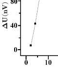
Figure 9: The potential difference $\rm\Delta U$ is generated by the ring current. It’s a function of the ring radius $\rm R_{surf}$.

References

- Yusa et al. (2021) N. Yusa, H. Song, D. Iwata, T. Uchimoto, T. Takagi, and M. Moroi, Nondestructive Testing and Evaluation 36, 1 (2021).
- Tuzlukov (2001) V. P. Tuzlukov, Signal detection theory (Springer Science & Business Media, 2001).
- Pastore and Scheirer (1974) R. Pastore and C. Scheirer, Psychological Bulletin 81, 945 (1974).
- Xifre-Perez et al. (2013) E. Xifre-Perez, L. Shi, U. Tuzer, R. Fenollosa, F. Ramiro-Manzano, R. Quidant, and F. Meseguer, ACS nano 7, 664 (2013).
- Yakushev (2013) E. Yakushev, in Advances in Imaging and Electron Physics, Vol. 178 (Elsevier, 2013) pp. 147–247.
- Zhao et al. (2021) Y. Zhao, J. Zhang, J. Li, S. Liu, P. Miao, Y. Shi, and E. Zhao, Measurement Science and Technology 32, 042002 (2021).
- Tian et al. (2022) B. Tian, S. Wen, X. Li, J. Ju, J. Tang, and N. Xiong, Applied Sciences 12, 10735 (2022).
- Brkovic et al. (1994) M. Brkovic, A. Pietkiewicz, and S. Cuk, in Proceedings of Intelec 94 (IEEE, 1994) pp. 155–162.
- Emig (2008) T. Emig, Journal of Statistical Mechanics: Theory and Experiment 2008, P04007 (2008).
- Essén and Fiolhais (2012) H. Essén and M. C. Fiolhais, American Journal of Physics 80, 164 (2012).
- Iverson and Kuhl (1995) P. Iverson and P. K. Kuhl, The Journal of the Acoustical Society of America 97, 553 (1995).
- Naitou et al. (1979) H. Naitou, S. Tokuda, and T. Kamimura, Journal of Computational Physics 33, 86 (1979).
- Charitat and Graner (2003) T. Charitat and F. Graner, European Journal of Physics 24, 267 (2003).
- Oliveira and Miranda (2001) M. H. Oliveira and J. A. Miranda, European Journal of Physics 22, 31 (2001).
- Albani and Bernardi (1974) M. Albani and P. Bernardi, IEEE Transactions on Microwave Theory and Techniques 22, 446 (1974).
- Árnason (1999) K. Árnason, in Three-Dimensional Electromagnetics (Society of Exploration Geophysicists, 1999) pp. 103–118.
- Bossavit (2005) A. Bossavit, in Numerical Methods in Electromagnetics, Handbook of Numerical Analysis, Vol. 13 (Elsevier, 2005) pp. 105–197.
- Bardeen (1955) J. Bardeen, Physical Review 97, 1724 (1955).
- Schafroth (1958) M. Schafroth, Physical Review 111, 72 (1958).
- Giuliani (2008) G. Giuliani, EPL (Europhysics Letters) 81, 60002 (2008).
- Galili et al. (2006) I. Galili, D. Kaplan, and Y. Lehavi, American journal of physics 74, 337 (2006).
- Uranga et al. (2004) A. Uranga, N. Lago, X. Navarro, and N. Barniol, in 2004 IEEE International Symposium on Circuits and Systems (IEEE Cat. No.04CH37512), Vol. 4 (2004) pp. IV–21.
- (23) S. GUIDE, Power 18, 11.
- Schilling and Shih (2019) P. Schilling and R. Shih, Parametric Modeling with SOLIDWORKS 2019 (SDC Publications, 2019).
- Akin (2010) J. E. Akin, Finite element analysis concepts: via SolidWorks (World Scientific, 2010).
- Avizienis and Kelly (1984) A. Avizienis and J. P. Kelly, Computer 17, 67 (1984).
- Bertoni et al. (2003) G. Bertoni, L. Breveglieri, I. Koren, P. Maistri, and V. Piuri, IEEE transactions on Computers 52, 492 (2003).
- Pan et al. (2020) D. Pan, S. Lin, L. Li, J. Li, Y. Jin, Z. Sun, and T. Liu, IEEE Transactions on Industrial Electronics 67, 1348 (2020).
- Shou et al. (2010) G. Shou, L. Xia, F. Liu, M. Zhu, Y. Li, and S. Crozier, IEEE Transactions on Magnetics 46, 1052 (2010).
- Evans et al. (2005) T. Evans, R. Moyer, J. Watkins, P. Thomas, T. Osborne, J. Boedo, M. Fenstermacher, K. Finken, R. Groebner, M. Groth, J. Harris, G. Jackson, R. L. Haye, C. Lasnier, M. Schaffer, G. Wang, and L. Zeng, Journal of Nuclear Materials 337-339, 691 (2005), pSI-16.
- Yu and Girshick (1991) B. W. Yu and S. L. Girshick, Journal of applied physics 69, 656 (1991).
- Anderson and Matthias (1964) P. Anderson and B. Matthias, Science 144, 373 (1964).
- Kaloper and Lawrence (2017) N. Kaloper and A. Lawrence, Physical Review D 95, 063526 (2017).
- Lax and Nelson (1976) M. Lax and D. Nelson, Physical Review B 13, 1777 (1976).
- Assous et al. (1993) F. Assous, P. Degond, E. Heintze, P. Raviart, and J. Segre, Journal of Computational Physics 109, 222 (1993).
- Gurevich and Laiho (1993) V. Gurevich and R. Laiho, Physical Review B 48, 8307 (1993).
- Gurevich et al. (1992) V. Gurevich, R. Laiho, and A. Lashkul, Physical review letters 69, 180 (1992).