Decentralized Bilevel Optimization

Abstract

Bilevel optimization has been successfully applied to many important machine learning problems. Algorithms for solving bilevel optimization have been studied under various settings. In this paper, we study the nonconvex-strongly-convex bilevel optimization under a decentralized setting. We design decentralized algorithms for both deterministic and stochastic bilevel optimization problems. Moreover, we analyze the convergence rates of the proposed algorithms in difference scenarios including the case where data heterogeneity is observed across agents. Numerical experiments on both synthetic and real data demonstrate that the proposed methods are efficient.

1 Introduction

Bilevel optimization provides a framework for solving problems arising from meta learning [33, 2, 29], hyperparameter optimization [26, 8], reinforcement learning[12], etc. It aims at minimizing an objective in the upper level under a constraint given by another optimization problem in the lower level, and has been studied intensively in recent years [8, 2, 9, 13, 12, 5]. Mathematically, it can be formulated as: x∈R^pΦ(x) = f(x,y^*(x)), (upper level) y^*(x) = arg min_y∈R^qg(x,y), (lower level) where $g$ is the lower level function which is usually assumed to be strongly convex with respect to $y$ for all $x$, and $f$ is the upper level function which is possibly non-convex. Designing a bilevel optimization algorithm typically consists of two parts: the lower loop and the upper loop. In the lower loop one can run algorithms like gradient descent on $y$ to find a good estimation of the global minimum of $g$ given $x$, which is guaranteed by the strong convexity of $g$. In the upper loop one can run gradient descent on $x$, which requires the estimation of the hypergradient $\nabla\Phi(x)$.

Decentralized optimization aims at solving the finite-sum problem: x∈R^p1n∑_i=1^nf_i(x), where the $i$-th agent only has access to the information related to $f_{i}$, and each agent communicates with neighbors so that they can cooperate to solve the original problem. There is no central server collecting local updates. Decentralized algorithms are better choices in certain scenarios [17, 34]. Since decentralized training has been proved to be efficient, it is natural to ask:

Can we design an algorithm to solve bilevel optimization problems in a decentralized regime?

We will see later that the answer is affirmative. Our contributions can be summarized as follows.

• We propose a novel algorithm that estimates the hypergradient in different cases.

• We design a decentralized bilevel optimization (DBO) algorithm and analyze its convergence rate. We also analyze the convergence results for the stochastic version of DBO. To the best of our knowledge, our paper is the first work proposing provably convergent decentralized bilevel optimization algorithms in the presence of data heterogeneity.

• We study the effect of gradient tracking in the deterministic decentralized bilevel optimization and analyze the convergence rates.

• We conduct numerical experiments on several hyperparameter optimization problems. The results demonstrate the efficiency of our algorithms.

1.1 Related work

Bilevel optimization can be dated back to [3]. Due to its great success in solving problems in meta learning [33, 2, 29] and hyperparameter optimization [26, 8], there is a flurry of work proposing and analyzing bilevel optimization algorithms. The major challenge in bilevel optimization is the estimation of the hypergradient $\nabla\Phi(x)$ in (1), which includes Jacobian and Hessian matrices in the closed-form expression. There are several strategies to overcome this: approximate implicit differentiation (AID) [7, 26, 10, 9, 11, 13], iterative differentiation (ITD) [7, 20, 8, 11, 13] and Neumann series-based approach [9, 5, 12, 13]. Provably convergent algorithms (both deterministic and stochastic cases) include BSA [9], TTSA [12], stocBiO [13], ALSET [5], to name a few.

Decentralized optimization plays a key role in distributed optimization. Under a decentralized setting, the data is distributed to different agents, and each agent communicates with neighbors to solve a finite-sum minimization problem. As opposed to centralized optimization, decentralized optimization aims at solving the problem without a central server that collects iterates from local agents. The main challenge is the data heterogeneity across agents, which should be mitigated by communications. It has been proved that decentralized algorithms have their own advantages [17] under certain circumstances, for example, low network bandwidth will greatly hinder the communication with the central server if the algorithm is designed to be centralized. An important approach to accelerate the decentralized algorithms is gradient tracking, which has been proved to be efficient [38, 6, 28, 23]. We refer the interested readers to [37], which provides a comprehensive review of decentralized optimization in a unified variance reduction framework.

There exist recent works considering bilevel optimization under distributed setting. Bilevel optimization under a federated setting has received some attention recently [35, 16], and so does min-max optimization under various distributed settings [36, 19, 31]. However, none of these papers considers bilevel optimization under the decentralized setting. We notice that there is a concurrent work [18] also studying decentralized bilevel optimization. However, it aims at solving decentralized bilevel optimization problems under a personalized learning setting, in a sense that the lower level problems are different among agents. In Section 3 we will see that our problem is substantially different from [18].

2 Preliminaries

In this paper we consider the following decentralized optimization problem: x∈R^pΦ(x) = 1n∑_i=1^nf_i(x,y^*(x)), (upper level) y^*(x) = arg min_y∈R^qg(x,y):= 1n∑_i=1^ng_i(x,y), (lower level) where $x\in\mathbb{R}^{p},y\in\mathbb{R}^{q}$. $f_{i}$ is possibly nonconvex and $g_{i}$ is strongly convex in $y$. Here $n$ denotes the number of agents, and agent $i$ only has access to information related to the local objective $f_{i}$:

$$f_{i}(x,y)=\mathbb{E}_{\phi\sim\mathcal{D}_{f_{i}}}\left[F(x,y;\phi)\right],\quad g_{i}(x,y)=\mathbb{E}_{\xi\sim\mathcal{D}_{g_{i}}}\left[G(x,y;\xi)\right].$$

In practice we can replace the expectation by empirical loss,

$$f_{i}(x,y)=\frac{1}{n_{f_{i}}}\sum_{j=1}^{n_{f_{i}}}F(x,y;\phi_{ij}),\quad g_{i}(x,y)=\frac{1}{n_{g_{i}}}\sum_{j=1}^{n_{g_{i}}}G(x,y;\xi_{ij}),$$

and then use mini-batch or full batch gradient descent in the updates. When we use mini-batch gradient descent, we call it "stochastic case", and when we use full batch gradient descent, we call it "deterministic case". We will study the convergence rates under these two cases in Section 3.

Notation. We denote by $\nabla f(x,y)$ and $\nabla^{2}f(x,y)$ the gradient and Hessian matrix of $f$, respectively. We use $\nabla_{x}f(x,y)$ and $\nabla_{y}f(x,y)$ to represent the gradients of $f$ with respect to $x$ and $y$, respectively. Denote by $\nabla_{xy}f(x,y)\in\mathbb{R}^{p\times q}$ the Jacobian matrix of $f$ and $\nabla_{y}^{2}f(x,y)$ the Hessian matrix of $f$ with respect to $y$. $\|\cdot\|$ denotes the $\ell_{2}$ norm for vectors and spectral norm for matrices, unless specified. $\mathbf{1}_{n}$ is the all one vector in $\mathbb{R}^{n}$, and $J_{n}=\mathbf{1}_{n}\mathbf{1}_{n}^{\mathsf{T}}$ is the $n\times n$ all one matrix.

The following assumptions will be used, which are standard in bilevel optimization [5, 9, 12, 13] and decentralized optimization literature [28, 23, 17, 34].

Assumption 2.1.

For any $i$, functions $f_{i}$, $\nabla f_{i}$, $\nabla g_{i}$, $\nabla^{2}g_{i}$ are $L_{f,0},L_{f,1},L_{g,1},L_{g,2}$ Lipschitz continuous respectively. Moreover, we define $L=\max\{L_{f,1},L_{g,1}\}$, and $\kappa=\frac{L}{\mu}$.

Assumption 2.2.

Function $g_{i}$ is $\mu$-strongly convex in $y$ for all $i$.

Assumption 2.3.

The weight matrix $W=(w_{ij})\in\mathbb{R}^{n\times n}$ is symmetric and doubly stochastic, i.e.:

$$W=W^{\mathsf{T}},\quad W\mathbf{1_{n}}=\mathbf{1_{n}},\quad w_{ij}\geq 0,\forall i,j,$$

and its eigenvalues satisfy $1=\lambda_{1}>\lambda_{2}\geq...\geq\lambda_{n}$ and $\rho:=\max\{|\lambda_{2}|,|\lambda_{n}|\}<1$.

Assumption 2.4.

(Data homogeneity on $g$) Assume the data associated with $g_{i}$ is independent and identically distributed, i.e., $\mathcal{D}_{g_{i}}=\mathcal{D}_{g}$. (Note that we do not require data homogeneity in the upper level function.)

For the stochastic algorithm in Section 3, we assume:

Assumption 2.5.

(Bounded variance) The stochastic derivatives $\nabla f_{i}(x,y;\phi)$, $\nabla g_{i}(x,y;\phi)$, $\nabla^{2}g_{i}(x,y;\phi)$ are unbiased with bounded variances $\sigma_{f}^{2}$, $\sigma_{g,1}^{2}$, $\sigma_{g,2}^{2}$, respectively.

3 Our Algorithms

Here we first discuss the main challenge when there is data heterogeneity, i.e., when Assumption 2.4 does not hold. Recall that in the outer loop, each node needs to estimate the hypergradient given by:

$$\nabla\Phi_{i}(x)=\nabla_{x}f_{i}(x,y^{*}(x))-\nabla_{xy}g(x,y^{*}(x))\left[\nabla_{y}^{2}g(x,y^{*}(x))\right]^{-1}\nabla_{y}f_{i}(x,y^{*}(x)).$$ (1)

Note that node $i$ only has access to $\nabla f_{i}$ and $\nabla g_{i}$ but it does not have access to $\nabla_{xy}g(x,y^{*}(x))\left[\nabla_{y}^{2}g(x,y^{*}(x))\right]^{-1}$ which requires the global information about $g$. One natural idea is to use (5) as a surrogate (here $y_{i}^{*}(x):=\operatorname*{arg\,min}_{y}g_{i}(x,y)$):

$$\nabla f_{i}(x,y_{i}^{*}(x))=\nabla_{x}f_{i}(x,y_{i}^{*}(x))-\nabla_{xy}g_{i}(x,y_{i}^{*}(x))\left[\nabla_{y}^{2}g_{i}(x,y_{i}^{*}(x))\right]^{-1}\nabla_{y}f_{i}(x,y_{i}^{*}(x)).$$ (2)

Unfortunately, this leads to the estimation for the error bound of

$$\left\|\left[\nabla^{2}g_{i}(x,y)\right]^{-1}-\left[\nabla^{2}g(x,y)\right]^{-1}\right\|,$$

which is not a diminishing term in the theoretical analysis without assuming the data homogeneity (Assumption 2.4). Mathematically, we would like to compute

$$\left[\sum_{i=1}^{n}\nabla_{xy}g_{i}(x,y)\right]\left[\sum_{i=1}^{n}\nabla_{y}^{2}g_{i}(x,y)\right]^{-1}$$

on node $i$ for any given $(x,y)$. In the next section we design a novel oracle to solve this subproblem with heterogeneous data at the price of the computation of Jacobian matrices.

3.1 Jacobian-Hessian-Inverse Product oracle

We first introduce the Jacobian-Hessian-Inverse Product (JHIP) oracle, which is essentially a decentralized algorithm. Denote by $H_{i}\in\mathbb{S}_{++}^{q\times q}$ and $J_{i}\in\mathbb{R}^{p\times q}$ the Hessian and Jacobian of $g_{i}$. Every agent would like to find $Z\in\mathbb{R}^{q\times p}$ such that:

$$\sum_{i=1}^{n}H_{i}Z=\sum_{i=1}^{n}J_{i}^{\mathsf{T}}\quad\text{or equivalently, }Z^{\mathsf{T}}=\left[\sum_{i=1}^{n}J_{i}\right]\left[\sum_{i=1}^{n}H_{i}\right]^{-1}.$$ (3)

Notice that this is exactly the optimality condition of:

$$\min_{Z\in\mathbb{R}^{p\times q}}\frac{1}{n}\sum_{i=1}^{n}h_{i}(Z),\quad\text{where }h_{i}(Z)=\frac{1}{2}\operatorname{Tr}{(Z^{\mathsf{T}}H_{i}Z)}-\operatorname{Tr}{(J_{i}Z)}.$$ (4)

The objective in (4) is strongly convex since each $H_{i}$ is symmetric positive definite. Hence we can design a decentralized algorithm with gradient tracking so that all the agents can collaborate to solve for (3) without a central server. The algorithm is described in Algorithm 1, where we use the bold texts to highlight the different updates when the problem is deterministic and stochastic.

Input: $Z_{i}^{(0)}\in\mathbb{R}^{q\times p}$, stepsizes $\{\gamma_{t}\}_{t=0}^{\infty}$, iteration number $N$, and initialization

• if deterministic, $Y_{i}^{(0)}=H_{i}Z_{i}^{(0)}-J_{i}^{\mathsf{T}},\mbox{ and }G_{i}^{(0)}=H_{i}Z_{i}^{(0)},$

• if stochastic, $Y_{i}^{(0)}=\hat{H}_{i}^{(0)}Z_{i}^{(0)}-\left[\hat{J}_{i}^{(0)}\right]^{\mathsf{T}},\mbox{ and }G_{i}^{(0)}=\hat{H}_{i}Z_{i}^{(0)}-\left[\hat{J}_{i}^{(0)}\right]^{\mathsf{T}}.$

1

Data: $H_{i}\in\mathbb{S}_{++}^{q\times q},J_{i}\in\mathbb{R}^{p\times q}$ accessible only to agent $i$ (deterministic).

  $(\hat{H}_{i}^{(t)},\hat{J}_{i}^{(t)}),t\in\{0,1,...,N-1\}$ accessible only to agent $i$ (stochastic).

2 for $t=0,1,...,N-1$ do

3       for $i=1,2,...,n$ do

4             $Z_{i}^{(t+1)}=\sum_{j=1}^{n}w_{ij}Z_{j}^{(t)}-\gamma_{t}Y_{i}^{(t)}$,

5             $G_{i}^{(t+1)}={H_{i}Z_{i}^{(t+1)}}$ if deterministic, or ${=\hat{H}_{i}^{(t+1)}Z_{i}^{(t+1)}-\left[\hat{J}_{i}^{(t+1)}\right]^{\mathsf{T}}}$ if stochastic,

6             $Y_{i}^{(t+1)}=\sum_{i=1}^{n}w_{ij}Y_{j}^{(t)}+G_{i}^{(t+1)}-G_{i}^{(t)}$.

7            

8       end for

9      

10 end for

Output: $Z_{i}^{(N)}$ on each node.

Algorithm 1 Jacobian-Hessian-Inverse Product oracle

Note that for the deterministic case we can just maintain $G_{i}^{(t+1)}=H_{i}Z_{i}^{(t+1)}$ instead of the gradient $H_{i}Z_{i}^{(t+1)}-J_{i}^{\mathsf{T}}$ because we only use $G_{i}^{(t+1)}$ in line 5 – the gradient tracking step, and the constant term $J_{i}^{\mathsf{T}}$ will be cancelled if we set $G_{i}^{(t+1)}$ as the gradient. We use $\hat{H}_{i}^{(t)}Z_{i}^{(t)}-\left[\hat{J}_{i}^{(t)}\right]^{\mathsf{T}}$ to represent the stochastic gradient of $h_{i}(Z)$ at $Z_{i}^{(t+1)}$. Although this oracle does not require Hessian computation for $H_{i}$, it still requires Jacobian oracle for $J_{i}$, which is more expensive than Jacobian-vector product oracle. Moreover, we have the convergence rates that have been well understood [28, 27, 37]. In general, one can also design other oracles (e.g., decentralized ADMM [22, 4, 32, 1, 21]) to solve (4). The convergence rates of this algorithm are summarized in Lemma A.13 in supplementary materials.

3.2 Hypergradient estimate

Input: $\nabla f_{i}(x,y),\nabla_{xy}g_{i}(x,y),\nabla_{y}^{2}g_{i}(x,y),N$.

Data: Samples $\phi=(\phi_{i}^{0},...,\phi_{i}^{(N+1)})$ on node $i$.

1 if Assumption 2.4 holds then

2       if Deterministic case then

3             Run $N$-step conjugate gradient method on $\left[\nabla_{y}^{2}g_{i}(x,y)\right]v=\nabla_{y}f_{i}(x,y)$ to get $v^{N}$.

4             Set $\hat{\nabla}f_{i}=\nabla_{x}f_{i}(x,y)-\nabla_{xy}g_{i}(x,y)v^{N}$  – AID based approach.

5       end if

6      if Stochastic case then

7             Set $\hat{\nabla}f_{i}=\nabla_{x}f_{i}(x,y;\phi^{(0)})-\nabla_{xy}g_{i}(x,y;\phi^{(1)})\cdot H\cdot\nabla_{y}f_{i}(x,y;\phi^{(0)})$, where $H=\left[\epsilon M\prod_{n=1}^{M^{\prime}}(I-\epsilon\nabla_{y}^{2}g_{i}(x,y;\phi^{(n+1)}))\right]$, and $M^{\prime}$ is drawn from $\{1,2,...,M\}$ uniformly at random  – Neumann series based approach.

8       end if

9      

10else

11       if Deterministic case then

12             Run $N$-step deterministic Algorithm 1 with $H_{i}=\nabla_{y}^{2}g_{i}(x,y),J_{i}=\nabla_{xy}g_{i}(x,y)$ and stepsize $\gamma_{t}=\gamma$ to get $Z_{i}^{(N)}$.

13             Set $\hat{\nabla}f_{i}=\nabla_{x}f_{i}(x,y)-\left[Z_{i}^{(N)}\right]^{\mathsf{T}}\nabla_{y}f_{i}(x,y)$  – deterministic JHIP.

14       end if

15      if Stochastic case then

16             Run $N$-step stochastic Algorithm 1 with $\hat{H}_{i}^{(t)}=\nabla_{y}^{2}g_{i}(x,y;\phi_{i}^{(t)}),\hat{J}_{i}^{(t)}=\nabla_{xy}g_{i}(x,y;\phi_{i}^{(t)})$ and $\gamma_{t}=\mathcal{O}(\frac{1}{t})$ to get $Z_{i}^{(N)}$.

17             Set $\hat{\nabla}f_{i}=\nabla_{x}f_{i}(x,y;\phi_{i}^{(0)})-\left[Z_{i}^{(N)}\right]^{\mathsf{T}}\nabla_{y}f_{i}(x,y;\phi_{i}^{(0)})$  – stochastic JHIP.

18       end if

19      

20 end if

Output: $\hat{\nabla}f_{i}$ on node $i$.

Algorithm 2 Hypergradient estimate

Before we propose our algorithms, we first introduce hypergradient estimates (Algorithm 2) under different cases.

• Case 1: Deterministic + homogeneous data. In this case the hypergradient is estimated based on the AID approach [13], which is essentially utilizing conjugate gradient method, and only requires Hessian-vector product oracles instead of explicit Hessian matrix computation. We adopt the approximation error (Lemma 3 in [13]) in Lemma A.9.

• Case 2: Stochastic + homogeneous data. In this case the hypergradient is estimated based on the Neumann series approach [9]. Gradients $\nabla f_{i}$ and $\nabla g_{i}$ are replaced by their corresponding first order stochastic oracles (i.e., stochastic gradients). We have the error estimation in Lemma A.32.

• Case 3: Heterogeneous data. In this case we compute the global Jacobian-Hessian-Inverse product by using the JHIP oracle (Algorithm 1). The error estimation results are given in Lemma A.12.

3.3 Deterministic decentralized bilevel optimization

Input: $W,N,K,T,\eta_{x},\eta_{y},x_{i,0},y_{i}^{(0)}$.

1 for $k=0,1,...,K-1$ do

2       $y_{i,k}^{(0)}=y_{i,k-1}^{(T)}\text{ if }k>0\text{ otherwise }y_{i,k}^{(0)}=y_{i}^{(0)}$.

3       for $t=0,1,...,T-1$ do

4             for $i=1,2,...,n$ do

5                   if Assumption 2.4 holds then

6                         $y_{i,k}^{(t+1)}=y_{i,k}^{(t)}-\eta_{y}\nabla_{y}g_{i}(x_{i,k},y_{i,k}^{(t)})$.

7                  else

8                         $v_{i,k}^{(t)}=\sum_{j=1}^{n}w_{ij}v_{j,k}^{(t-1)}+\nabla_{y}g_{i}(x_{i,k},y_{i,k}^{(t)})-\nabla_{y}g_{i}(x_{i,k},y_{i,k}^{(t-1)})$.

9                         $y_{i,k}^{(t+1)}=\sum_{j=1}^{n}w_{ij}y_{j,k}^{(t)}-\eta_{y}v_{i,k}^{(t)}$.

10                   end if

11                  

12             end for

13            

14       end for

15      for $i=1,2,...,n$ do

16             Run Algorithm 2 (with "deterministic case" option) and set the output as $\hat{\nabla}f_{i}(x_{i,k},y_{i,k}^{(T)})$.

17             $x_{i,k+1}=\sum_{j=1}^{n}w_{ij}x_{j,k}-\eta_{x}\hat{\nabla}f_{i}(x_{i,k},y_{i,k}^{(T)})$.

18       end for

19      

20 end for

Algorithm 3 (Deterministic) Decentralized Bilevel Optimization

We propose the decentralized bilevel optimization algorithm (DBO) in Algorithm 3. In the inner loop (lines 3-9) each agent performs local gradient descent updates for variable $y$ in parallel (line 4-8). When Assumption 2.4 holds, we can simply run local gradient descent without communication because in the lower level local distribution already captures the global function information. When Assumption 2.4 does not hold, then the data distribution is substantially heterogeneous across agents, so we add weighted averaging steps (line 9) to reach consensus and gradient tracking steps (line 8) to reduce the complexity. In the outer loop (lines 11-14) each agent communicates with neighbors and then performs gradient descent for variable $x$. For simplicity we use constant stepsize $\eta_{x}$ in the outer loop. Similar results can be obtained for diminishing stepsizes. Using proper parameters, we have the following sublinear convergence results of Algorithm 3 for solving the deterministic problem.

Theorem 3.1.

In Algorithm 3, suppose Assumptions 2.1, 2.2, and 2.3 hold. If Assumption 2.4 holds, we set $\eta_{x}=\Theta(K^{-\frac{1}{3}}n^{-\frac{1}{3}}\kappa^{-\frac{8}{3}}),\ \eta_{y}\leq\frac{2}{\mu+L},\ T=\Theta(\log(\kappa)),\ N=\Theta(\log(\kappa))$. If Assumption 2.4 does not hold, we set $\eta_{x}=\Theta(K^{-\frac{1}{3}}n^{-\frac{1}{3}}\kappa^{-\frac{8}{3}}),\ \eta_{y}^{(t)}=\mathcal{O}(1),\ T=\Theta(\log K),\ N=\Theta(\log K)$. In both cases, we have: $\frac{1}{K+1}\sum_{j=0}^{K}\|\nabla\Phi(\overline{x_{j}})\|^{2}=\mathcal{O}\left(\frac{n^{\frac{1}{3}}\kappa^{\frac{8}{3}}}{K^{\frac{2}{3}}}\right),$ where $\overline{x_{j}}=\frac{1}{n}\sum_{i=1}^{n}x_{i,j}$.

This convergence rate matches the previous results in nonconvex decentralized optimization [17, 34]. We conjecture that the bound $N=\Theta(\log K)$ in the second case is not tight, and can be improved by using a technique similar to the case when Assumption 2.4 holds. We leave this as a future work.

3.4 Deterministic decentralized bilevel optimization with gradient tracking

In this section we study the effect of gradient tracking in decentralized bilevel optimization. We propose the Decentralized Bilevel Optimization with Gradient Tracking (DBOGT) Algorithm 4. We introduce $u$ and $v$ to serve as the update direction. Gradient tracking technique has been widely used in distributed optimization literature [6, 28, 23]. The effect of adding such a direction accelerates the algorithm in a sense that one can choose a constant stepsize that is independent of the iteration number. For Algorithm 4 we have the following theorem.

Input: $W,N,K,T,\eta_{x},\eta_{y},x_{i}^{(0)},y_{i}^{(0)}$.

1 for $k=0,1,...,K-1$ do

2       $y_{i,k}^{(0)}=y_{i,k-1}^{(T)}\text{ if }k>0\text{ otherwise }y_{i,k}^{(0)}=y_{i}^{(0)}$.

3       for $t=0,1,...,T-1$ do

4             for $i=1,2,...,n$ do

5                   if Assumption 2.4 holds then

6                         $y_{i,k}^{(t+1)}=y_{i,k}^{(t)}-\eta_{y}\nabla_{y}g_{i}(x_{i,k},y_{i,k}^{(t)})$.

7                  else

8                         $v_{i,k}^{(t)}=\sum_{j=1}^{n}w_{ij}v_{j,k}^{(t-1)}+\nabla_{y}g_{i}(x_{i,k},y_{i,k}^{(t)})-\nabla_{y}g_{i}(x_{i,k},y_{i,k}^{(t-1)})$.

9                         $y_{i,k}^{(t+1)}=\sum_{j=1}^{n}w_{ij}y_{j,k}^{(t)}-\eta_{y}v_{i,k}^{(t)}$.

10                   end if

11                  

12             end for

13            

14       end for

15      for $i=1,2,...,n$ do

16             Run Algorithm 2 (with "deterministic case" option) and set the output as $\hat{\nabla}f_{i}(x_{i,k},y_{i,k}^{(T)})$.

17             $u_{i,k}=\sum_{j=1}^{n}w_{ij}u_{j,k-1}+\hat{\nabla}f_{i}(x_{i,k},y_{i,k}^{(T)})-\hat{\nabla}f_{i}(x_{i,k-1},y_{i,k-1}^{(T)})$.

18             $x_{i,k+1}=\sum_{j=1}^{n}w_{ij}x_{j,k}-\eta_{x}u_{i,k}$.

19       end for

20      

21 end for

Algorithm 4 (Deterministic) Decentralized Bilevel Optimization with Gradient Tracking

Theorem 3.2.

In Algorithm 4, suppose Assumptions 2.1, 2.2, and 2.3 hold. If Assumption 2.4 holds, we set $\eta_{x}=\Theta(\kappa^{-3}),\ \eta_{y}\leq\frac{2}{\mu+L},\ T=\Theta(\log(\kappa)),\ N=\Theta(\log(\kappa))$. If Assumption 2.4 does not hold, we set $\eta_{x}=\Theta(\kappa^{-3}),\ \eta_{y}=\Theta(1),\ N=\Theta(\log K),\ T=\Theta(\log K)$. In both cases, we have $\frac{1}{K+1}\sum_{j=0}^{K}\|\nabla\Phi(\overline{x_{j}})\|^{2}=\mathcal{O}\left(\frac{1}{K}\right),$ where $\overline{x_{j}}=\frac{1}{n}\sum_{i=1}^{n}x_{i,j}$.

Note that this result implies that in DBOGT we can set $\eta_{x}$ as a constant that is independent of the total number of iterations $K$, which matches the results in gradient tracking literature [28, 23, 14].

3.5 Decentralized stochastic bilevel optimization

Our stochastic version of the DBO algorithm: Decentralized Stochastic Bilevel Optimization (DSBO), is described in Algorithm 5. Its convergence rate is given in Theorem 3.3.

Input: $W,N,K,T,\eta_{x},\eta_{y},x_{i}^{(0)},y_{i}^{(0)}$.

1 for $k=0,1,...,K-1$ do

2       $y_{i,k}^{(0)}=y_{i,k-1}^{(T)}\text{ if }k>0\text{ otherwise }y_{i,k}^{(0)}=y_{i}^{(0)}$.

3       for $t=0,1,...,T-1$ do

4             for $i=1,2,...,n$ do

5                   if Assumption 2.4 holds then

6                         $y_{i,k}^{(t+1)}=y_{i,k}^{(t)}-\eta_{y}\nabla_{y}g_{i}(x_{i,k},y_{i,k}^{(t)};\xi_{i,k}^{(t)})$.

7                  else

8                         $y_{i,k}^{(t+1)}=\sum_{j=1}^{n}w_{ij}y_{j,k}^{(t)}-\eta_{y}^{(t)}\nabla_{y}g_{i}(x_{i,k},y_{i,k}^{(t)};\xi_{i,k}^{(t)})$.

9                   end if

10                  

11             end for

12            

13       end for

14      for $i=1,2,...,n$ do

15             Run Algorithm 2 (with "stochastic case" option) and set the output as $\hat{\nabla}f_{i}(x_{i,k},y_{i,k}^{(T)};\phi_{i,k})$.

16             $x_{i,k+1}=\sum_{j=1}^{n}w_{ij}x_{j,k}-\eta_{x}\hat{\nabla}f_{i}(x_{i,k},y_{i,k}^{(T)};\phi_{i,k})$.

17       end for

18      

19 end for

Algorithm 5 Decentralized Stochastic Bilevel Optimization

Theorem 3.3.

In Algorithm 5, suppose Assumptions 2.1, 2.2, and 2.3 hold. If Assumption 2.4 holds, we set $M=\Theta(\log(K),\ T=\Theta(\log(\kappa)),\ \epsilon<\frac{1}{L},\ \eta_{x}=\Theta(K^{-\frac{1}{2}}),\ \eta_{y}=\Theta(K^{-\frac{1}{2}})$. If Assumption 2.4 does not hold, we set $\eta_{x}=\Theta(K^{-\frac{1}{2}}),\ \eta_{y}=\Theta(K^{-\frac{1}{2}}),\ T=\Theta(K^{\frac{1}{2}}),\ N=\Theta(\log K)$. In both cases, we have $\frac{1}{K+1}\sum_{j=0}^{K}\mathbb{E}\left[\|\nabla\Phi(\overline{x_{j}})\|^{2}\right]=\mathcal{O}(\frac{1}{\sqrt{K}}),$ where $\overline{x_{j}}=\frac{1}{n}\sum_{i=1}^{n}x_{i,j}$.

4 Numerical experiments

In this section we conduct several experiments on hyperparameter optimization problems in the decentralized setting, which can be formulated as: λ∈R^pΦ(λ) = 1n∑_i=1^nf_i(λ, τ^*(λ)), τ^*(λ) = arg min_τ∈R^q 1n∑_i=1^ng_i(λ, τ). Here $f_{i}$ and $g_{i}$ denote the validation loss and training loss on node $i$, respectively. The goal is to find the best hyperparameter $\lambda$ under the constraint that $\tau^{*}(\lambda)$ is the optimal model parameter of the lower level problem. For each experiment, we set our network topology as a special ring network, where $W=(w_{i,j})$ and the only nonzero elements are given by:

$$w_{i,i}=a,\ w_{i,i+1}=w_{i,i-1}=\frac{1-a}{2},\ \text{ for some }a\in(0,1).$$

Here we overload the notation and set $w_{n,n+1}=w_{n,1},w_{1,0}=w_{1,n}$. Note that $a$ is the unique parameter that determines the weight matrix and will be specified in each experiment.

4.1 Synthetic data

We first conduct logistic regression with $l^{2}$ regularization on synthetic heterogeneous data (e.g., [26], [11]). On node $i$ we have:

$$f_{i}(\lambda,\tau^{*}(\lambda))=\sum_{(x_{e},y_{e})\in\mathcal{D}_{i}^{\prime}}\psi(y_{e}x_{e}^{\mathsf{T}}\tau^{*}(\lambda)),$$

$$g_{i}(\lambda,\tau)=\sum_{(x_{e},y_{e})\in\mathcal{D}_{i}}\psi(y_{e}x_{e}^{\mathsf{T}}\tau)+\frac{1}{2}\tau^{\mathsf{T}}\text{diag}(e^{\lambda})\tau,$$

where $e^{\lambda}$ is element-wise, $\text{diag}(v)$ denotes the diagonal matrix generated by vector $v$, and $\psi(x)=\log(1+e^{-x})$. $\mathcal{D}_{i}^{\prime}$ and $D_{i}$ represent validation set and training set on node $i$. Following the setup in [11], we first randomly generate $\tau^{*}\in\mathbb{R}^{p}$ and the noise vector $\epsilon\in\mathbb{R}^{p}$. For the data point $(x_{e},y_{e})$ on node $i$, each element of $x_{e}$ is sampled from the normal distribution with mean 0, variance $i^{2}$. $y_{e}$ is then set by $y_{e}=\text{sign}(x_{e}^{\mathsf{T}}\tau^{*}+m\epsilon)$, where sign denotes the sign function and $m=0.1$ denotes the noise rate. In the experiment we choose $p=q=50,$ and the number of inner-loop and outer-loop iterations as $10$ and $100$ respectively. $N,$ the number of iterations of the JHIP oracle 1 is $20$. The stepsizes are $\eta_{x}=\eta_{y}=\gamma=0.01.$ The number of agents $n$ is chosen as $20,$ and the weight parameter $a=0.4$. We plot the logarithm of the norm of the gradient in Figure 1(a). From this figure we see that all three algorithms: DBO (Algorithm 3), DBOGT (Algorithm 4), and DSBO (Algorithm 5) can reduce the gradient to an acceptable level. Moreover, DBO and DBOGT have similar performance, and they are both slightly better than DSBO.

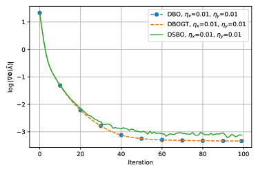
(a) Logistic regression on synthetic data.

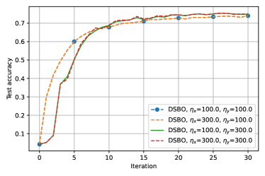
(b) Logistic regression on 20 Newsgroup dataset.

Figure 1:

4.2 Real-world data

We now conduct the DSBO algorithm on a logistic regression problem on 20 Newsgroup dataset[11]. On node $i$ we have:

$$f_{i}(\lambda,\tau^{*}(\lambda))=\frac{1}{|\mathcal{D}^{(i)}_{val}|}\sum_{(x_{e},y_{e})\in\mathcal{D}^{(i)}_{val}}L(x_{e}^{\mathsf{T}}\tau^{*},y_{e}),$$

$$g_{i}(\lambda,\tau)=\frac{1}{|D_{tr}^{(i)}|}\sum_{(x_{e},y_{e})\in\mathcal{D}^{(i)}_{tr}}L(x_{e}^{\mathsf{T}}\tau,y_{e})+\frac{1}{cp}\sum_{i=1}^{c}\sum_{j=1}^{p}e^{\lambda_{j}}\tau_{ij}^{2},$$

where $c=20$ denotes the number of topics, $p=101631$ is the feature dimension, $L$ is the cross entropy loss, $\mathcal{D}_{val}$ and $\mathcal{D}_{tr}$ are the validation and training data sets, respectively. Our codes can be seen as decentralized versions of the one provided in [13]. We first set inner and outer stepsizes $\eta_{x}=\eta_{y}=100$ (the same as the ones used in [13]), and then compare its performance with different stepsizes. We set the number of inner-loop iterations $T=10,$ the number of outer-loop iterations $K=30,$ the number of agents $n=20,$ and the weight parameter $a=0.33$. At the end of $j$-th outer-loop iteration we use the average $\overline{\tau_{j}}=\frac{1}{n}\sum_{i=1}^{n}\tau_{i,j}$ as the model parameter and then do the classification on the test set to get the test accuracy. In Figure 1(b) we plot the test accuracy of every iteration. From this figure we see that the DSBO algorithm is able to get good test accuracy under different settings of stepsizes.

Finally we apply deterministic DBO and DBOGT algorithms on a data hyper-cleaning problem [30, 13] for MNIST dataset [15]. The purpose is to demonstrate the advantage of the gradient tracking technique. On node $i$ we have:

$$f_{i}(\lambda,\tau) =\frac{1}{|\mathcal{D}^{(i)}_{val}|}\sum_{(x_{e},y_{e})\in\mathcal{D}^{(i)}_{val}}L(x_{e}^{\mathsf{T}}\tau,y_{e}),$$

$$g_{i}(\lambda,\tau) =\frac{1}{|D^{(i)}_{tr}|}\sum_{(x_{e},y_{e})\in\mathcal{D}^{(i)}_{tr}}\sigma(\lambda_{e})L(x_{e}^{\mathsf{T}}\tau,y_{e})+C_{r}\|\tau\|^{2},$$

where $L$ is the cross-entropy loss and $\sigma(x)=(1+e^{-x})^{-1}$ is the sigmoid function. The number of inner-loop iterations $T$ and outer-loop iterations $K$ are set as $10$ and $30$, respectively. The number of agents $n=20$ and the weight parameter $a=0.5$. Following [30, 13] the regularization parameter $C_{r}$ is set as $0.001$. We first choose stepsizes similar to those in[13] and then set larger stepsizes. In each iteration we evaluate the norm of the hypergradient at the average of the hyperparameters $\bar{\lambda}$, and plot the logarithm (base 10) of the norm of the hypergradient versus iteration number in Figure 2. The Figure 2 shows that the perofromance of DBO and DBOGT are similar when the stepsizes are small. However, the Figure 2 shows that DBOGT converges much faster than DBO when the stepsizes are relatively large. This supports the conclusions in Theorem 3.2.

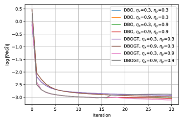
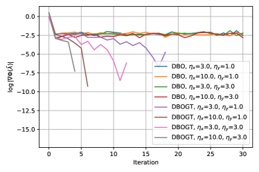
Figure 2: (a) and (b): Data hyper-cleaning on MNIST

5 Conclusion

In this paper we propose both deterministic and stochastic algorithms for solving decentralized bilevel optimization problems. We obtain sublinear convergence rates when the lower level function is generated by homogeneous data. Moreover, at the price of computing Jacobian matrices, we propose decentralized algorithms with sublinear convergence rates when the lower level function is generated by heterogeneous data. Numerical experiments demonstrate that the proposed algorithms are efficient. It is still an open question whether one can design decentralized optimization algorithms without assuming data homogeneity and deterministic (or stochastic) Jacobian computation. We leave this as a future work.

Appendix A Appendix

Convergence analysis

In this section we provide the proofs of convergence results. For convenience, we first list the notation below.

• $W:=(w_{ij})\in\mathbb{R}^{n\times n}$ is symmetric doubly stochastic, and $\rho:=\max\{|\lambda_{2}|,|\lambda_{n}|\}<1$.

• $X_{k}:=[x_{1,k},x_{2,k},...,x_{n,k}]\in\mathbb{R}^{p\times n}$.

• $\overline{x_{k}}:=\frac{1}{n}\sum_{i=1}^{n}x_{i,k}\in\mathbb{R}^{p}$.

• $\partial\Phi(X_{k}):=[\hat{\nabla}f_{1}(x_{1,k},y_{1,k}^{(T)}),\hat{\nabla}f_{2}(x_{2,k},y_{2,k}^{(T)}),...,\hat{\nabla}f_{n}(x_{n,k},y_{n,k}^{(T)})]\in\mathbb{R}^{p\times n}$.

• $\overline{\partial\Phi(X_{k})}:=\frac{1}{n}\sum_{i=1}^{n}\hat{\nabla}f_{i}(x_{i,k},y_{i,k}^{(T)})$.

• $\partial\Phi(X_{k};\phi):=[\hat{\nabla}f_{1}(x_{1,k},y_{1,k}^{(T)};\phi_{1,k}),\hat{\nabla}f_{2}(x_{2,k},y_{2,k}^{(T)};\phi_{2,k}),...,\hat{\nabla}f_{n}(x_{n,k},y_{n,k}^{(T)};\phi_{n,k})]\in\mathbb{R}^{p\times n}$.

• $\overline{\partial\Phi(X_{k};\phi)}:=\frac{1}{n}\sum_{i=1}^{n}\hat{\nabla}f_{i}(x_{i,k},y_{i,k}^{(T)};\phi_{i,k})$.

• $q_{i,k}:=x_{i,k}-\overline{x_{k}}=X_{k}(e_{i}-\frac{\mathbf{1}_{n}}{n})$.

• $Q_{k}:=[q_{1,k},q_{2,k},...,q_{n,k}]\in\mathbb{R}^{p\times n}$. Assume $x_{i,0}=0$ and thus $Q_{0}=0$.

• $r_{i,k}:=u_{i,k}-\overline{u_{k}}$.

• $R_{k}:=\left[r_{1,k},r_{2,k},...,r_{n,k}\right]\in\mathbb{R}^{p\times n}$.

• $S_{K}:=\sum_{k=1}^{K}\|Q_{k}\|^{2}$.

• $T_{K}:=\sum_{j=0}^{K}\|\nabla\Phi(\overline{x_{j}})\|^{2}$.

• $E_{K}:=\sum_{j=1}^{K}\sum_{i=1}^{n}\|x_{i,j}-x_{i,j-1}\|^{2}$.

• When Assumption 2.4 holds, define:

  $$A_{K}:=\sum_{j=0}^{K}\sum_{i=1}^{n}\|y_{i,j}^{(T)}-y_{i}^{*}(x_{i,j})\|^{2},B_{K}:=\sum_{j=0}^{K}\sum_{i=1}^{n}\|v_{i,j}^{*}-v_{i,j}^{(0)}\|^{2},$$

  where

  $$v_{i,j}^{*}=\left[\nabla_{y}^{2}g_{i}(x_{i,j},y_{i}^{*}(x_{i,j}))\right]^{-1}\nabla_{y}f_{i}(x_{i,j},y_{i}^{*}(x_{i,j})).$$

• $\delta_{y}^{T}:=(1-\frac{2\eta_{y}\mu L}{\mu+L})^{T}$, $\delta_{\kappa}^{N}:=(\frac{\sqrt{\kappa}-1}{\sqrt{\kappa}+1})^{2N}$.

We first introduce a few lemmas that are useful in the proofs. The following lemma gives bounds for matrix $2$-norm.

Lemma A.1.

For any given matrix $A=(a_{1},a_{2},...,a_{q})\in\mathbb{R}^{p\times q}$, we have:

$$\|a_{j}\|^{2}\leq\|A\|^{2}\leq\sum_{i=1}^{q}\|a_{i}\|^{2},\ \forall{j}\in\{1,2,...,q\}.$$

The following lemma is a common result in decentralized optimization (e.g., [17, Lemma 4]).

Lemma A.2.

Under Assumption 2.3 we have:

$$\left\|W^{k}-\frac{J_{n}}{n}\right\|\leq\rho^{k},\ \forall k\in\{0,1,2,...\}.$$

Proof.

Assume $1=\lambda_{1}>\lambda_{2}\geq...\geq\lambda_{n}>-1$ are eigenvalues of $W$. Since $W^{k}J_{n}=J_{n}W^{k}$, we know $W^{k}$ and $J_{n}$ are simultaneously diagonalizable. Hence there exists an orthogonal matrix $P$ such that

$$W^{k}=P\text{diag}(\lambda_{i}^{k})P^{-1},\quad\frac{J_{n}}{n}=P\text{diag}(1,0,0,...,0)P^{-1},$$

and thus:

$$\left\|W^{k}-\frac{J_{n}}{n}\right\|=\|P(\text{diag}(\lambda_{i}^{k})-\text{diag}(1,0,0,...,0))P^{-1}\|\leq\max\{|\lambda_{2}|^{k},|\lambda_{n}|^{k}\}=\rho^{k}.$$

∎

The following three lemmas are adopted from Lemma 2.2 in [9]:

Lemma A.3.

(Hypergradient) Define $\Phi_{i}(x):=f_{i}(x,y^{*}(x))$, where $y^{*}(x)=\operatorname*{arg\,min}_{y\in\mathbb{R}^{q}}g(x,y)$. Under Assumptions 2.1 and 2.2 we have:

$$\nabla\Phi_{i}(x)=\nabla_{x}f_{i}(x,y^{*}(x))-\nabla_{xy}g(x,y^{*}(x))\left[\nabla_{y}^{2}g(x,y^{*}(x))\right]^{-1}\nabla_{y}f_{i}(x,y^{*}(x)).$$

Moreover, $\nabla\Phi_{i}$ is Lipschitz continuous:

$$\|\nabla\Phi_{i}(x_{1})-\nabla\Phi_{i}(x_{2})\|\leq L_{\Phi}\|x_{1}-x_{2}\|,$$

with the Lipschitz constant given by:

$$L_{\Phi}=L+\frac{2L^{2}+L_{g,2}L_{f,0}^{2}}{\mu}+\frac{LL_{f,0}L_{g,2}+L^{3}+L_{g,2}L_{f,0}L}{\mu^{2}}+\frac{L_{g,2}L^{2}L_{f,0}}{\mu^{3}}=\Theta(\kappa^{3}).$$

Remark: if Assumption 2.4 does not hold, then this hypergradient is completely different from the local hypergradient:

$$\nabla f_{i}(x,y_{i}^{*}(x))=\nabla_{x}f_{i}(x,y_{i}^{*}(x))-\nabla_{xy}g_{i}(x,y_{i}^{*}(x))\left[\nabla_{y}^{2}g_{i}(x,y_{i}^{*}(x))\right]^{-1}\nabla_{y}f_{i}(x,y_{i}^{*}(x)),$$ (5)

where $y_{i}^{*}(x)=\operatorname*{arg\,min}_{y\in\mathbb{R}^{q}}g_{i}(x,y)$.

Lemma A.4.

Define:

$$\bar{\nabla}f_{i}(x,y)=\nabla_{x}f_{i}(x,y)-\nabla_{xy}g(x,y)\left[\nabla_{y}^{2}g(x,y)\right]^{-1}\nabla_{y}f_{i}(x,y).$$

Under the Assumption 2.1 we have:

$$\|\bar{\nabla}f_{i}(x,y)-\bar{\nabla}f_{i}(\tilde{x},\tilde{y})\|\leq L_{f}\|(x,y)-(\tilde{x},\tilde{y})\|,$$

where the Lipschitz constant is given by:

$$L_{f}=L+\frac{L^{2}}{\mu}+L_{f,0}\left[\frac{L_{g,2}}{\mu}+\frac{L_{g,2}L}{\mu^{2}}\right]=\Theta(\kappa^{2}).$$

Lemma A.5.

Suppose Assumptions 2.1 and 2.2 hold, then we have:

$$\|y_{i}^{*}(x_{1})-y_{i}^{*}(x_{2})\|\leq\kappa\|x_{1}-x_{2}\|,\quad\forall i\in\{1,2,...,n\}.$$

These lemmas basically reveal some nice properties of functions in bilevel optimization under Assumptions 2.1 and 2.2. We will make use of these lemmas in our theoretical analysis.

Lemma A.6.

If the iterates satisfy:

$$\overline{x_{k+1}}=\overline{x_{k}}-\eta_{x}\overline{\partial\Phi(X_{k})},\quad\text{where }0<\eta_{x}\leq\frac{1}{L_{\Phi}},$$

then we have the following inequality holds:

$$\frac{1}{K+1}\sum_{k=0}^{K}\|\nabla\Phi(\overline{x_{k}})\|^{2}\leq\frac{2}{\eta_{x}(K+1)}(\Phi(\overline{x_{0}})-\inf_{x}\Phi(x))+\frac{1}{K+1}\sum_{k=0}^{K}\|\overline{\partial\Phi(X_{k})}-\nabla\Phi(\overline{x_{k}})\|^{2}.$$ (6)

Proof.

Since $\Phi(x)$ is $L_{\Phi}$-smooth, we have:

$$\Phi(\overline{x_{k+1}})-\Phi(\overline{x_{k}})\leq\nabla\Phi(\overline{x_{k}})^{\mathsf{T}}(-\eta_{x}\overline{\partial\Phi(X_{k})})+\frac{L_{\Phi}\eta_{x}^{2}}{2}\|\overline{\partial\Phi(X_{k})}\|^{2}=\frac{L_{\Phi}\eta_{x}^{2}}{2}\|\overline{\partial\Phi(X_{k})}\|^{2}-\eta_{x}\nabla\Phi(\overline{x_{k}})^{\mathsf{T}}\overline{\partial\Phi(X_{k})}$$

$$= \frac{L_{\Phi}\eta_{x}^{2}}{2}\|\overline{\partial\Phi(X_{k})}-\nabla\Phi(\overline{x_{k}})\|^{2}+(\frac{L_{\Phi}\eta_{x}^{2}}{2}-\eta_{x})\|\nabla\Phi(\overline{x_{k}})\|^{2}+(L_{\Phi}\eta_{x}^{2}-\eta_{x})\nabla\Phi(\overline{x_{k}})^{\mathsf{T}}(\overline{\partial\Phi(X_{k})}-\nabla\Phi(\overline{x_{k}}))$$

$$\leq \frac{L_{\Phi}\eta_{x}^{2}}{2}\|\overline{\partial\Phi(X_{k})}-\nabla\Phi(\overline{x_{k}})\|^{2}+(\frac{L_{\Phi}\eta_{x}^{2}}{2}-\eta_{x})\|\nabla\Phi(\overline{x_{k}})\|^{2}+(\eta_{x}-L_{\Phi}\eta_{x}^{2})(\frac{1}{2}\|\overline{\partial\Phi(X_{k})}-\nabla\Phi(\overline{x_{k}})\|^{2}+\frac{1}{2}\|\nabla\Phi(\overline{x_{k}})\|^{2})$$

$$= \frac{\eta_{x}}{2}\|\overline{\partial\Phi(X_{k})}-\nabla\Phi(\overline{x_{k}})\|^{2}-\frac{\eta_{x}}{2}\|\nabla\Phi(\overline{x_{k}})\|^{2},$$

where the second inequality is due to Young’s inequality and $\eta_{x}\leq\frac{1}{L_{\Phi}}$. Therefore, we have:

$$\|\nabla\Phi(\overline{x_{k}})\|^{2} \leq\frac{2}{\eta_{x}}(\Phi(\overline{x_{k}})-\Phi(\overline{x_{k+1}}))+\|\overline{\partial\Phi(X_{k})}-\nabla\Phi(\overline{x_{k}})\|^{2}.$$ (7)

Summing (7) over $k=0,\ldots,K$, yields:

$$\sum_{k=0}^{K}\|\nabla\Phi(\overline{x_{k}})\|^{2}\leq\frac{2}{\eta_{x}}(\Phi(\overline{x_{0}})-\Phi(\overline{x_{K+1}}))+\sum_{k=0}^{K}\|\overline{\partial\Phi(X_{k})}-\nabla\Phi(\overline{x_{k}})\|^{2},$$

which completes the proof. ∎

We have the following lemma which provides an upper bound for $E_{K}$:

Lemma A.7.

In each iteration, if we have $\overline{x_{k+1}}=\overline{x_{k}}-\eta_{x}\overline{\partial\Phi(X_{k})}$, then the following inequality holds:

$$E_{K}\leq 8nS_{K}+4n\eta_{x}^{2}\sum_{j=0}^{K-1}\|\overline{\partial\Phi(X_{j})}-\nabla\Phi(\overline{x_{j}})\|^{2}+4n\eta_{x}^{2}T_{K-1}.$$

Proof.

By the definition of $E_{K}$, we have:

$$E_{K}= \sum_{j=1}^{K}\sum_{i=1}^{n}\|x_{i,j}-x_{i,j-1}\|^{2}=\sum_{j=1}^{K}\sum_{i=1}^{n}\|x_{i,j}-\overline{x_{j}}+\overline{x_{j}}-\overline{x_{j-1}}+\overline{x_{j-1}}-x_{i,j-1}\|^{2}$$

$$= \sum_{j=1}^{K}\sum_{i=1}^{n}\|q_{i,j}-\eta_{x}(\overline{\partial\Phi(X_{j-1})}-\nabla\Phi(\overline{x_{j-1}}))-\eta_{x}\nabla\Phi(\overline{x_{j-1}})-q_{i,j-1}\|^{2}$$

$$\leq 4\sum_{j=1}^{K}\sum_{i=1}^{n}(\|q_{i,j}\|^{2}+\eta_{x}^{2}\|\overline{\partial\Phi(X_{j-1})}-\nabla\Phi(\overline{x_{j-1}}))\|^{2}+\eta_{x}^{2}\|\nabla\Phi(\overline{x_{j-1}})\|^{2}+\|q_{i,j-1}\|^{2})$$

$$\leq 4n\sum_{j=1}^{K}(\|Q_{j}\|^{2}+\|Q_{j-1}\|^{2}+\eta_{x}^{2}\|\overline{\partial\Phi(X_{j-1})}-\nabla\Phi(\overline{x_{j-1}})\|^{2}+\eta_{x}^{2}\|\nabla\Phi(\overline{x_{j-1}})\|^{2})$$

$$\leq 8nS_{K}+4n\eta_{x}^{2}\sum_{j=0}^{K-1}(\|\overline{\partial\Phi(X_{j})}-\nabla\Phi(\overline{x_{j}})\|^{2}+\|\nabla\Phi(\overline{x_{j}})\|^{2})$$

$$= 8nS_{K}+4n\eta_{x}^{2}\sum_{j=0}^{K-1}\|\overline{\partial\Phi(X_{j})}-\nabla\Phi(\overline{x_{j}})\|^{2}+4n\eta_{x}^{2}T_{K-1},$$

where the second inequality is by the definition of $Q_{j}$, the third inequality is by the definition of $S_{K}$ and $Q_{0}=0$, the last equality is by the definition of $T_{K-1}.$ ∎

Next we give bounds for $A_{K}$ and $B_{K}$.

Lemma A.8.

Under Assumption 2.4, if we properly choose $\eta_{y},T$ and $N$ in Algorithm 3 and 4 such that:

$$\eta_{y}\leq\frac{2}{\mu+L},\quad\delta_{y}^{T}<\frac{1}{3},\quad\delta_{\kappa}^{N}<\frac{1}{8\kappa},$$ (8)

then the following inequalities hold:

$$A_{K}\leq 3\delta_{y}^{T}(c_{1}+2\kappa^{2}E_{K}),\quad B_{K}\leq 2c_{2}+2d_{1}A_{K-1}+2d_{2}E_{K},$$

where the constants are defined as follows:

$$c_{1}=\sum_{i=1}^{n}\|y_{i,0}^{(0)}-y_{i}^{*}(x_{i,0})\|^{2},\ c_{2}=\sum_{i=1}^{n}\|v_{i,0}^{*}-v_{i,0}^{(0)}\|^{2},$$ (9)

$$d_{1}=4(1+\sqrt{\kappa})^{2}(\kappa+\frac{L_{g,2}L_{f,0}}{\mu^{2}})^{2}=\Theta(\kappa^{5}),\ d_{2}=2(\kappa^{2}+\frac{2L_{f,0}\kappa}{\mu}+\frac{2L_{f,0}\kappa^{2}}{\mu})^{2}=\Theta(\kappa^{6}).$$

Proof.

Recall that $A_{K}:=\sum_{j=0}^{K}\sum_{i=1}^{n}\|y_{i,j}^{(T)}-y_{i}^{*}(x_{i,j})\|^{2}$. In order to bound $A_{K}$, we bound each term as follows.

$$\|y_{i,j}^{(T)}-y_{i}^{*}(x_{i,j})\|^{2}=\|y_{i,j}^{(T-1)}-\eta_{y}\nabla_{y}g(x_{i,j},y_{i,j}^{(T-1)})-y_{i}^{*}(x_{i,j})\|^{2}$$ (10)

$$= \|y_{i,j}^{(T-1)}-y_{i}^{*}(x_{i,j})\|^{2}-2\eta_{y}\nabla_{y}g_{i}(x_{i,j},y_{i,j}^{(T-1)})^{\mathsf{T}}(y_{i,j}^{(T-1)}-y_{i}^{*}(x_{i,j}))+\eta_{y}^{2}\|\nabla_{y}g_{i}(x_{i,j},y_{i,j}^{(T-1)})\|^{2}$$

$$\leq (1-\frac{2\eta_{y}\mu L}{\mu+L})\|y_{i,j}^{(T-1)}-y_{i}^{*}(x_{i,j})\|^{2}+\eta_{y}(\eta_{y}-\frac{2}{\mu+L})\|\nabla_{y}g_{i}(x_{i,j},y_{i,j}^{(T-1)})\|^{2}$$

$$\leq (1-\frac{2\eta_{y}\mu L}{\mu+L})\|y_{i,j}^{(T-1)}-y_{i}^{*}(x_{i,j})\|^{2}$$

$$\leq (1-\frac{2\eta_{y}\mu L}{\mu+L})^{T}\|y_{i,j}^{(0)}-y_{i}^{*}(x_{i,j})\|^{2}$$

$$= \delta_{y}^{T}\|y_{i,j}^{(0)}-y_{i}^{*}(x_{i,j})\|^{2},$$

where the first inequality follows from the strong-convexity and smoothness of the function $g$ [24, Theorem 2.1.12], and the second inequality holds since we have $\eta_{y}\leq\frac{2}{\mu+L}$. We further have:

$$\|y_{i,j}^{(0)}-y_{i}^{*}(x_{i,j})\|^{2}=\|y_{i,j-1}^{(T)}-y_{i}^{*}(x_{i,j-1})+y_{i}^{*}(x_{i,j-1})-y_{i}^{*}(x_{i,j})\|^{2}$$

$$\leq 2(\|y_{i,j-1}^{(T)}-y_{i}^{*}(x_{i,j-1})\|^{2}+\|y_{i}^{*}(x_{i,j-1})-y_{i}^{*}(x_{i,j})\|^{2})$$

$$\leq 2\delta_{y}^{T}\|y_{i,j-1}^{(0)}-y_{i}^{*}(x_{i,j-1})\|^{2}+2\kappa^{2}\|x_{i,j-1}-x_{i,j}\|^{2}$$

$$< \frac{2}{3}\|y_{i,j-1}^{(0)}-y_{i}^{*}(x_{i,j-1})\|^{2}+2\kappa^{2}\|x_{i,j-1}-x_{i,j}\|^{2},$$

where the second inequality is by (10) and Lemma A.5, and the last inequality is by the condition (8). Taking summation on both sides, we get

$$\sum_{j=1}^{K}\sum_{i=1}^{n}\|y_{i,j}^{(0)}-y_{i}^{*}(x_{i,j})\|^{2}$$

$$\leq \frac{2}{3}\sum_{j=1}^{K}\sum_{i=1}^{n}\|y_{i,j-1}^{(0)}-y_{i}^{*}(x_{i,j-1})\|^{2}+2\kappa^{2}\sum_{j=1}^{K}\sum_{i=1}^{n}\|x_{i,j}-x_{i,j-1}\|^{2}$$

$$\leq \frac{2}{3}\sum_{j=0}^{K}\sum_{i=1}^{n}\|y_{i,j}^{(0)}-y_{i}^{*}(x_{i,j})\|^{2}+2\kappa^{2}E_{K}$$

$$\leq \frac{2}{3}c_{1}+\frac{2}{3}\sum_{j=1}^{K}\sum_{i=1}^{n}\|y_{i,j}^{(0)}-y_{i}^{*}(x_{i,j})\|^{2}+2\kappa^{2}E_{K},$$

which directly implies:

$$\sum_{j=1}^{K}\sum_{i=1}^{n}\|y_{i,j}^{(0)}-y_{i}^{*}(x_{i,j})\|^{2}\leq 2c_{1}+6\kappa^{2}E_{K}.$$ (11)

Combining (10) and (11) leads to:

$$A_{K}=\sum_{j=0}^{K}\sum_{i=1}^{n}\|y_{i,j}^{T}-y_{i}^{*}(x_{i,j})\|^{2}\leq\delta_{y}^{T}\sum_{j=0}^{K}\sum_{i=1}^{n}\|y_{i,j}^{(0)}-y_{i}^{*}(x_{i,j})\|^{2}$$

$$\leq\delta_{y}^{T}(c_{1}+2c_{1}+6\kappa^{2}E_{K})=3\delta_{y}^{T}(c_{1}+2\kappa^{2}E_{K}).$$

We then consider the bound for $B_{K}$. Recall that:

$$v_{i,k}^{*}=\left[\nabla_{y}^{2}g_{i}(x_{i,k},y_{i}^{*}(x_{i,k}))\right]^{-1}\nabla_{y}f_{i}(x_{i,k},y_{i}^{*}(x_{i,k})),$$

which is the solution of the linear system $\left[\nabla_{y}^{2}g_{i}(x_{i,k},y_{i}^{*}(x_{i,k}))\right]v=\nabla_{y}f_{i}(x_{i,k},y_{i}^{*}(x_{i,k}))$ in the AID-based approach in Algorithm 2. Note that $v_{i,k}^{*}$ is a function of $x_{i,k}$, and it is $(\kappa^{2}+\frac{2L_{f,0}L}{\mu^{2}}+\frac{2L_{f,0}L\kappa}{\mu^{2}})$-Lipschitz continuous with respect to $x_{i,k}$ [13]. For each term in $B_{K}$, we have:

$$\|v_{i,j}^{*}-v_{i,j}^{(0)}\|^{2} \leq 2(\|v_{i,j-1}^{*}-v_{i,j-1}^{(N)}\|^{2}+\|v_{i,j}^{*}-v_{i,j-1}^{*}\|^{2})$$

$$\leq 4(1+\sqrt{\kappa})^{2}(\kappa+\frac{L_{g,2}L_{f,0}}{\mu^{2}})^{2}\|y_{i,j-1}^{(T)}-y_{i}^{*}(x_{i,j-1})\|^{2}$$

$$+4\kappa(\frac{\sqrt{\kappa}-1}{\sqrt{\kappa}+1})^{2N}\|v_{i,j-1}^{*}-v_{i,j-1}^{(0)}\|^{2}+2(\kappa^{2}+\frac{2L_{f,0}L}{\mu^{2}}+\frac{2L_{f,0}L\kappa}{\mu^{2}})^{2}\|x_{i,j}-x_{i,j-1}\|^{2},$$

where the second inequality follows [13, Lemma 4]. Taking summation over $i,j$, we get

$$\sum_{j=1}^{K}\sum_{i=1}^{n}\|v_{i,j}^{*}-v_{i,j}^{(0)}\|^{2}\leq d_{1}A_{K-1}+4\kappa\delta_{\kappa}^{N}B_{K-1}+d_{2}E_{K}\leq d_{1}A_{K-1}+\frac{1}{2}B_{K}+d_{2}E_{K},$$ (12)

where the last inequality holds since we pick $N$ such that $4\kappa\delta_{\kappa}^{N}<\frac{1}{2}$. Therefore, we can get:

$$B_{K}\leq c_{2}+d_{1}A_{K-1}+\frac{1}{2}B_{K}+d_{2}E_{K}\quad\Rightarrow\quad B_{K}\leq 2c_{2}+2d_{1}A_{K-1}+2d_{2}E_{K},$$

which completes the proof. ∎

The following lemmas give bounds on $\sum\|\overline{\partial\Phi(X_{k})}-\nabla\Phi(\overline{x_{k}})\|^{2}$ in (7).We first consider the case when the Assumption 2.4 holds. In this case, the outer loop computes the hypergradient via AID based approach. Therefore, we borrow [13, Lemma 3] and restate it as follows.

Lemma A.9.

[13, Lemma 3] Suppose Assumptions 2.1, 2.2, and 2.4 hold, then we have:

$$\|\hat{\nabla}f_{i}(x_{i,j},y_{i,j}^{(T)})-\nabla f_{i}(x,y_{i}^{*}(x))\|^{2}\leq\Gamma\|y_{i}^{*}(x_{i,j})-y_{i,j}^{(T)}\|^{2}+6L^{2}\kappa\left(\frac{\sqrt{\kappa}-1}{\sqrt{\kappa}+1}\right)^{2N}\|v_{i,j}^{*}-v_{i,j}^{(0)}\|^{2},$$

where the constant $\Gamma$ is

$$\Gamma=3L^{2}+\frac{3L_{g,2}^{2}L_{f,0}}{\mu^{2}}+6L^{2}(1+\sqrt{\kappa})^{2}\left(\kappa+\frac{L_{g,2}L_{f,0}}{\mu^{2}}\right)^{2}=\Theta(\kappa^{5}).$$

Next, we are ready to bound $\sum\|\overline{\partial\Phi(X_{k})}-\nabla\Phi(\overline{x_{k}})\|^{2}$ when Assumption 2.4 holds.

Lemma A.10.

Under Assumption 2.4, we have:

$$\sum_{k=0}^{K}\|\overline{\partial\Phi(X_{k})}-\nabla\Phi(\overline{x_{k}})\|^{2}\leq 2L_{\Phi}^{2}S_{K}+\frac{2\Gamma}{n}A_{K}+\frac{12L^{2}\kappa}{n}\delta_{\kappa}^{N}B_{K}.$$ (13)

Proof.

Under Assumption 2.4 we know $g_{i}=g$, and thus from (1) and (2) we have

$$\nabla\Phi_{i}(\overline{x_{k}})=\nabla f_{i}(\overline{x_{k}},y^{*}(\overline{x_{k}})).$$

Therefore, we have

$$\|\overline{\partial\Phi(X_{k})}-\nabla\Phi(\overline{x_{k}})\|^{2}=\frac{1}{n^{2}}\left\|\sum_{i=1}^{n}\left[\hat{\nabla}f_{i}(x_{i,k},y_{i,k}^{(T)})-\nabla f_{i}(\overline{x_{k}},y^{*}(\overline{x_{k}}))\right]\right\|^{2}$$

$$\leq \frac{1}{n}\sum_{i=1}^{n}\|\hat{\nabla}f_{i}(x_{i,k},y_{i,k}^{(T)})-\nabla f_{i}(\overline{x_{k}},y^{*}(\overline{x_{k}}))\|^{2}$$

$$\leq \frac{2}{n}\sum_{i=1}^{n}(\|\hat{\nabla}f_{i}(x_{i,k},y_{i,k}^{(T)})-\nabla f_{i}(x_{i,k},y_{i}^{*}(x_{i,k}))\|^{2}+\|\nabla f_{i}(x_{i,k},y_{i}^{*}(x_{i,k}))-\nabla f_{i}(\overline{x_{k}},y^{*}(\overline{x_{k}}))\|^{2})$$

$$\leq \frac{2}{n}\sum_{i=1}^{n}(\Gamma\|y_{i}^{*}(x_{i,k})-y_{i,k}^{(T)}\|^{2}+6L^{2}\kappa\delta_{\kappa}^{N}\|v_{i,k}^{*}-v_{i,k}^{(0)}\|^{2}+\|\nabla f_{i}(x_{i,k},y^{*}(x_{i,k}))-\nabla f_{i}(\overline{x_{k}},y^{*}(\overline{x_{k}}))\|^{2})$$

$$\leq \frac{2\Gamma}{n}\sum_{i=1}^{n}\|y_{i}^{*}(x_{i,k})-y_{i,k}^{(T)}\|^{2}+\frac{12L^{2}\kappa}{n}\delta_{\kappa}^{N}\sum_{i=1}^{n}\|v_{i,k}^{*}-v_{i,k}^{(0)}\|^{2}+2L_{\Phi}^{2}\|Q_{k}\|^{2},$$

where the first inequality follows from the convexity of $\|\cdot\|^{2}$, the third inequality follows from Lemma A.9 and Assumption 2.4, the last inequality is by Lemma A.3:

$$\|\nabla f_{i}(x_{i,k},y^{*}(x_{i,k}))-\nabla f_{i}(\overline{x_{k}},y^{*}(\overline{x_{k}}))\|^{2}=\|\nabla\Phi_{i}(x_{i,k})-\nabla\Phi_{i}(\overline{x_{k}})\|^{2}$$

$$\leq L_{\Phi}^{2}\|x_{i,k}-\overline{x_{k}}\|^{2}=L_{\Phi}^{2}\|q_{i,k}\|^{2}\leq L_{\Phi}^{2}\|Q_{k}\|^{2}.$$

Taking summation on both sides, we get:

$$\sum_{k=0}^{K}\|\overline{\partial\Phi(X_{k})}-\nabla\Phi(\overline{x_{k}})\|^{2}\leq 2L_{\Phi}^{2}S_{K}+\frac{2\Gamma}{n}A_{K}+\frac{12L^{2}\kappa}{n}\delta_{\kappa}^{N}B_{K}.$$ (14)

∎

We now consider the case when Assumption 2.4 does not hold. In this case, our target in the lower level problem is

$$y^{*}(\overline{x_{k}})=\operatorname*{arg\,min}_{y}\frac{1}{n}\sum_{i=1}^{n}g_{i}(\overline{x_{k}},y).$$ (15)

However, the update in our decentralized algorithm (e.g. line 8 of Algorithm 3) aims at solving

$$\tilde{y}_{k}^{*}:=\operatorname*{arg\,min}_{y}\frac{1}{n}\sum_{i=1}^{n}g_{i}(x_{i,k},y),$$ (16)

which is completely different from our target (15). To resolve this problem, we introduce the following lemma to characterize the difference:

Lemma A.11.

The following inequality holds:

$$\|\tilde{y}_{k}^{*}-y^{*}(\overline{x_{k}})\|\leq\frac{\kappa}{n}\sum_{i=1}^{n}\|x_{i,k}-\overline{x_{k}}\|\leq\kappa\|Q_{k}\|.$$

Proof.

By optimality conditions of (15) and (16), we have:

$$\frac{1}{n}\sum_{i=1}^{n}\nabla_{y}g_{i}(x_{i,k},\tilde{y}_{k}^{*})=0,\quad\frac{1}{n}\sum_{i=1}^{n}\nabla_{y}g_{i}(\overline{x_{k}},y^{*}(\overline{x_{k}}))=0.$$

Combining with the strongly convexity and the smoothness of $g_{i}$ yields:

$$\|\frac{1}{n}\sum_{i=1}^{n}\nabla_{y}g_{i}(\overline{x_{k}},\tilde{y}_{k}^{*})\|=\|\frac{1}{n}\sum_{i=1}^{n}\nabla_{y}g_{i}(\overline{x_{k}},\tilde{y}_{k}^{*})-\frac{1}{n}\sum_{i=1}^{n}\nabla_{y}g_{i}(\overline{x_{k}},y^{*}(\overline{x_{k}}))\|\geq\mu\|\tilde{y}_{k}^{*}-y^{*}(\overline{x_{k}})\|,$$

$$\|\frac{1}{n}\sum_{i=1}^{n}\nabla_{y}g_{i}(\overline{x_{k}},\tilde{y}_{k}^{*})\|=\|\frac{1}{n}\sum_{i=1}^{n}\nabla_{y}g_{i}(\overline{x_{k}},\tilde{y}_{k}^{*})-\frac{1}{n}\sum_{i=1}^{n}\nabla_{y}g_{i}(x_{i,k},\tilde{y}_{k}^{*})\|\leq\frac{L}{n}\sum_{i=1}^{n}\|x_{i,k}-\overline{x_{k}}\|.$$

Therefore, we obtain the following inequality:

$$\|\tilde{y}_{k}^{*}-y^{*}(\overline{x_{k}})\|\leq\frac{\kappa}{n}\sum_{i=1}^{n}\|x_{i,k}-\overline{x_{k}}\|=\frac{\kappa}{n}\sum_{i=1}^{n}\|q_{i,k}\|\leq\kappa\|Q_{k}\|,$$

where the last inequality is by Lemma A.1. ∎

Notice that in the inner loop of Algorithms 3, 4 and 5, i.e., Lines 4-11 of Algorithms 3 and 4, and Lines 4-10 of Algorithm 5, $y_{i,k}^{T}$ converges to $\tilde{y}_{k}^{*}$ and the rates are characterized by [25, 27, 37, 28] (e.g., Corollary 4.7. in [25], Theorem 10 in [23] and Theorem 1 in [27]). We include all the convergence rates here.

Lemma A.12.

Suppose Assumption 2.4 does not hold. We have:

• In Algorithm 3 there exists $\eta_{y}^{(t)}=\mathcal{O}(\frac{1}{t})$ such that $\frac{1}{n}\sum_{i=1}^{n}\|y_{i,k}^{(T)}-\tilde{y}_{k}^{*}\|^{2}\leq\frac{C_{1}}{T}$;

• In Algorithm 4 there exists a constant $\eta_{y}$ such that $\frac{1}{n}\sum_{i=1}^{n}\|y_{i,k}^{(T)}-\tilde{y}_{k}^{*}\|^{2}\leq C_{2}\alpha_{1}^{T}$;

• In Algorithm 5 there exists $\eta_{y}^{(t)}=\mathcal{O}(\frac{1}{t})$ such that $\frac{1}{n}\sum_{i=1}^{n}\mathbb{E}\left[\|y_{i,k}^{(T)}-\tilde{y}_{k}^{*}\|^{2}\right]\leq\frac{C_{3}}{T}$.

Here $C_{1},C_{2},C_{3}$ are positive constant and $\alpha_{1}\in(0,1)$.

Besides, the JHIP oracle (Algorithm 1) also performs standard decentralized optimization with gradient tracking in deterministic case (Algorithms 3 and 4) and stochastic case (Algorithm 5). We have:

Lemma A.13.

In Algorithm 1, we have:

• For deterministic case, there exists a constant $\gamma$ such that if $\gamma_{t}\equiv\gamma$ then $\|Z_{i}^{(t)}-Z^{*}\|^{2}\leq C_{4}\alpha_{2}^{t}$. (See [28]).

• For stochastic case and there exists a diminishing stepsize sequence $\gamma_{t}=\mathcal{O}(\frac{1}{t})$, such that $\frac{1}{n}\sum_{i=1}^{n}\mathbb{E}\left[\|Z_{i}^{(t)}-Z^{*}\|^{2}\right]\leq\frac{C_{5}}{t}$. (See [37]).

Here $C_{4},C_{5}$ are positive constant, and $\alpha_{2}\in(0,1)$. Here the optimal solution is denoted by $(Z^{*})^{\mathsf{T}}=\left[\sum_{i=1}^{n}J_{i}\right]\left[\sum_{i=1}^{n}H_{i}\right]^{-1}$.

For simplicity we define:

$$C=\max\{C_{1},C_{2},C_{3},C_{4},C_{5}\},\quad\alpha=\max\{\alpha_{1},\alpha_{2}\}.$$

Since the objective functions mentioned in Lemma A.12 (the lower level function $g$) and A.13 (the objective in (4)) are strongly convex, we know $C$ and $\alpha$ only depend on $L,\mu,\rho$ and the stepsize (only when it is a constant). For example $\alpha_{2}$ in Lemma A.13 only depends on the spectral radius of $H_{i}$, smallest eigenvalue of $H_{i}$, $\rho$ and $\gamma$.
For heterogeneous data on $g$ we have a different error estimation.

Lemma A.14.

Suppose Assumption 2.4 does not hold. In Algorithm 3 and 4 we have:

$$\|\hat{\nabla}f_{i}(x_{i,k},y_{i,k}^{(T)})-\bar{\nabla}f_{i}(x_{i,k},\tilde{y}_{k}^{*})\|^{2}\leq 3L^{2}(1+\kappa^{2})\|y_{i,k}^{(T)}-\tilde{y}_{k}^{*}\|^{2}+3L_{f,0}^{2}C\alpha^{N}.$$ (17)

Proof.

Note that:

$$\hat{\nabla}f_{i}(x_{i,k},y_{i,k}^{(T)}) =\nabla_{x}f_{i}(x_{i,k},y_{i,k}^{(T)})-\left[Z_{i,k}^{(N)}\right]^{\mathsf{T}}\nabla_{y}f_{i}(x_{i,k},y_{i,k}^{(T)}),$$

$$\bar{\nabla}f_{i}(x_{i,k},\tilde{y}_{k}^{*}) =\nabla_{x}f_{i}(x_{i,k},\tilde{y}_{k}^{*})-\nabla_{xy}g(x_{i,k},\tilde{y}_{k}^{*})\nabla_{y}^{2}g(x_{i,k},\tilde{y_{k}}^{*})^{-1}\nabla_{y}f_{i}(x_{i,k},\tilde{y}_{k}^{*}).$$

Then we know:

$$\|\hat{\nabla}f_{i}(x_{i,k},y_{i,k}^{(T)})-\bar{\nabla}f_{i}(x_{i,k},\tilde{y}_{k}^{*}))\|^{2}\leq 3\|\nabla_{x}f_{i}(x_{i,k},y_{i,k}^{(T)})-\nabla_{x}f_{i}(x_{i,k},\tilde{y}_{k}^{*})\|^{2}$$

$$+3\left\|\left[\left[Z_{i,k}^{(N)}\right]^{\mathsf{T}}-\nabla_{xy}g(x_{i,k},\tilde{y}_{k}^{*})\nabla_{y}^{2}g(x_{i,k},\tilde{y_{k}}^{*})^{-1}\right]\nabla_{y}f_{i}(x_{i,k},y_{i,k}^{(T)})\right\|^{2}$$

$$+3\left\|\nabla_{xy}g(x_{i,k},\tilde{y}_{k}^{*})\nabla_{y}^{2}g(x_{i,k},\tilde{y_{k}}^{*})^{-1}\left[\nabla_{y}f_{i}(x_{i,k},y_{i,k}^{(T)})-\nabla_{y}f_{i}(x_{i,k},\tilde{y}_{k}^{*})\right]\right\|^{2}$$

$$\leq 3L^{2}\|y_{i,k}^{(T)}-\tilde{y}_{k}^{*}\|^{2}+3L_{f,0}^{2}C\alpha^{N}+3L^{2}\kappa^{2}\|y_{i,k}^{(T)}-\tilde{y}_{k}^{*}\|^{2}$$

$$=3L^{2}(1+\kappa^{2})\|y_{i,k}^{(T)}-\tilde{y}_{k}^{*}\|^{2}+3L_{f,0}^{2}C\alpha^{N}.$$

Notice that we have: $[Z_{i,k}^{*}]^{\mathsf{T}}=\nabla_{xy}g(x_{i,k},\tilde{y}_{k}^{*})\nabla_{y}^{2}g(x_{i,k},\tilde{y_{k}}^{*})^{-1}$, so the second inequality is by Assumption 2.1 and Lemma A.13. ∎

Lemma A.15.

Suppose Assumption 2.4 does not hold, then in Algorithms 3 and 4 we have:

$$\|\overline{\partial\Phi(X_{k})}-\nabla\Phi(\overline{x_{k}})\|^{2}\leq 6(L^{2}(1+\kappa^{2}))C\alpha^{T}+6L_{f,0}^{2}C\alpha^{N}+2(L_{f}^{2}+L_{f}^{2}\kappa^{2})\|Q_{k}\|^{2}.$$ (18)

Proof.

We have

$$\|\overline{\partial\Phi(X_{k})}-\nabla\Phi(\overline{x_{k}})\|^{2}=\frac{1}{n^{2}}\|\sum_{i=1}^{n}\left[\hat{\nabla}f_{i}(x_{i,k},y_{i,k}^{(T)})-\nabla f_{i}(\overline{x_{k}},y^{*}(\overline{x_{k}}))\right]\|^{2}$$

$$\leq \frac{1}{n}\sum_{i=1}^{n}\|\hat{\nabla}f_{i}(x_{i,k},y_{i,k}^{(T)})-\nabla f_{i}(\overline{x_{k}},y^{*}(\overline{x_{k}}))\|^{2}$$

$$\leq \frac{2}{n}\sum_{i=1}^{n}(\|\hat{\nabla}f_{i}(x_{i,k},y_{i,k}^{(T)})-\bar{\nabla}f_{i}(x_{i,k},\tilde{y}_{k}^{*}))\|^{2}+\|\bar{\nabla}f_{i}(x_{i,k},\tilde{y}_{k}^{*})-\nabla f_{i}(\overline{x_{k}},y^{*}(\overline{x_{k}}))\|^{2})$$

$$\leq \frac{2}{n}\sum_{i=1}^{n}(3(L^{2}(1+\kappa^{2}))\|y_{i,k}^{(T)}-\tilde{y}_{k}^{*}\|^{2}+3L_{f,0}^{2}C\alpha^{N}+L_{f}^{2}\|x_{i,k}-\overline{x_{k}}\|^{2}+L_{f}^{2}\|\tilde{y}_{k}^{*}-y^{*}(\overline{x_{k}})\|^{2})$$

$$\leq \frac{2}{n}\sum_{i=1}^{n}(3(L^{2}(1+\kappa^{2}))\|y_{i,k}^{(T)}-\tilde{y}_{k}^{*}\|^{2}+3L_{f,0}^{2}C\alpha^{N}+L_{f}^{2}\|q_{i,k}\|^{2}+L_{f}^{2}\kappa^{2}\|Q_{k}\|^{2})$$

$$= \frac{6(L^{2}(1+\kappa^{2}))}{n}\sum_{i=1}^{n}\|y_{i,k}^{(T)}-\tilde{y}_{k}^{*}\|^{2}+6L_{f,0}^{2}C\alpha^{N}+2(L_{f}^{2}+L_{f}^{2}\kappa^{2})\|Q_{k}\|^{2},$$

where the third inequality is due to Lemma A.14 and Lemma A.4, the last inequality is by Lemma A.11. Notice that $\frac{1}{n}\sum_{i=1}^{n}\|y_{i,k}^{(T)}-\tilde{y}_{k}^{*}\|^{2}$ in the first term denotes the error of the inner loop iterates. In both DBO (Algorithm 3) and DBOGT (Algorithm 4), the inner loop performs a decentralized gradient descent with gradient tracking. By Lemma A.12, we have the error bound $\frac{1}{n}\sum_{i=1}^{n}\|y_{i,k}^{(T)}-\tilde{y}_{k}^{*}\|^{2}\leq C\alpha^{T}$, which completes the proof. ∎

A.1 Proof of the DBO convergence

In this section we will prove the following convergence result of the DBO algorithm:

Theorem A.16.

In Algorithm 3, suppose Assumptions 2.1, 2.2, and 2.3 hold. If Assumption 2.4 holds, then by setting $\eta_{x}\leq\frac{1-\rho}{130\sqrt{n}L_{\Phi}},\ \eta_{y}\leq\frac{2}{\mu+L},\ T=\Theta(\log(\kappa)),\ N=\Theta(\log(\kappa))$, we have:

$$\frac{1}{K+1}\sum_{j=0}^{K}\|\nabla\Phi(\overline{x_{j}})\|^{2}\leq\frac{4}{\eta_{x}(K+1)}(\Phi(\overline{x_{0}})-\inf_{x}\Phi(x))+n\eta_{x}^{2}\cdot\frac{1272L_{\Phi}^{2}L_{f,0}^{2}(1+\kappa)^{2}}{(1-\rho)^{2}}+\frac{C_{1}}{K+1}.$$

If Assumption 2.4 does not hold, then by setting $\eta_{x}\leq\frac{1}{L_{\Phi}},\eta_{y}^{(t)}=\mathcal{O}(\frac{1}{t})$, we have:

$$\frac{1}{K+1}\sum_{j=0}^{K}\|\nabla\Phi(\overline{x_{j}})\|^{2}\leq\frac{2}{\eta_{x}(K+1)}(\Phi(\overline{x_{0}})-\inf_{x}\Phi(x))+\eta_{x}^{2}\frac{4nL_{f}^{2}(1+\kappa^{2})L_{f,0}^{2}}{(1-\rho)^{2}}((1+\kappa)^{2}+C\alpha^{N})+\tilde{C_{1}},$$

where $C_{1}=\Theta(1),C=\Theta(1)$ and $\tilde{C_{1}}=\mathcal{O}(\alpha^{T}+\alpha^{N})$.

We first consider bounding the consensus error estimation for DBO:

Lemma A.17.

In Algorithm 3, we have

$$S_{K}:=\sum_{k=1}^{K}\|Q_{k}\|^{2} <\frac{\eta_{x}^{2}}{(1-\rho)^{2}}\sum_{j=0}^{K-1}\sum_{i=1}^{n}\|\hat{\nabla}f_{i}(x_{i,j},y_{i,j}^{(T)})\|^{2}.$$

Proof.

Note that the $x$ update can be written as

$$X_{k}=X_{k-1}W-\eta_{x}\partial\Phi(X_{k-1}),$$

which indicates

$$\overline{x_{k}}=\overline{x_{k-1}}-\eta_{x}\overline{\partial\Phi(X_{k-1})}.$$

By definition of $q_{i,k}$, we have

$$q_{i,k+1} =\sum_{j=1}^{n}w_{ij}x_{j,k}-\eta_{x}\hat{\nabla}f(x_{i,k},y_{i,k}^{(T)})-(\overline{x_{k}}-\eta_{x}\overline{\partial\Phi(X_{k})})$$

$$=\sum_{j=1}^{n}w_{ij}(x_{j,k}-\overline{x_{k}})-\eta_{x}(\hat{\nabla}f(x_{i,k},y_{i,k}^{(T)})-\overline{\partial\Phi(X_{k})})$$

$$=Q_{k}We_{i}-\eta_{x}\partial\Phi(X_{k})(e_{i}-\frac{\mathbf{1}_{n}}{n})\quad\text{ -- $W$ is symmetric.}$$

Therefore, the update for the matrix $Q_{k+1}$ is

$$Q_{k+1} =Q_{k}W-\eta_{x}\partial\Phi(X_{k})(I-\frac{J_{n}}{n})$$

$$=(Q_{k-1}W-\eta_{x}\partial\Phi(X_{k-1})(I-\frac{J_{n}}{n}))W-\eta_{x}\partial\Phi(X_{k})(I-\frac{J_{n}}{n})$$

$$=Q_{0}W^{k+1}-\eta_{x}\sum_{i=0}^{k}(\partial\Phi(X_{i})(I-\frac{J_{n}}{n})W^{k-i})$$

$$=-\eta_{x}\sum_{i=0}^{k}\partial\Phi(X_{i})(W^{k-i}-\frac{J_{n}}{n}),$$

where the last equality is obtained by $Q_{0}=0$ and $J_{n}W=J_{n}.$ By Cauchy-Schwarz inequality, we have the following estimate

$$\|Q_{k+1}\|^{2} =\eta_{x}^{2}\|\sum_{i=0}^{k}\partial\Phi(X_{i})(W^{k-i}-\frac{J_{n}}{n})\|^{2}$$

$$\leq\eta_{x}^{2}(\sum_{i=0}^{k}\rho^{k-i}\|\partial\Phi(X_{i})\|^{2})(\sum_{i=0}^{k}\frac{1}{\rho^{k-i}}\|W^{k-i}-\frac{J_{n}}{n}\|^{2})$$

$$\leq\eta_{x}^{2}(\sum_{i=0}^{k}\rho^{k-i}\|\partial\Phi(X_{i})\|^{2})(\sum_{i=0}^{k}\rho^{k-i})$$

$$<\frac{\eta_{x}^{2}}{1-\rho}(\sum_{i=0}^{k}\rho^{k-i}\|\partial\Phi(X_{i})\|^{2}),$$

where the second inequality is obtained by Lemma A.2. Recall the definition of $\partial\Phi(X_{k})$:

$$\partial\Phi(X_{k})=[\hat{\nabla}f_{1}(x_{1,k},y_{1,k}^{(T)}),\hat{\nabla}f_{2}(x_{2,k},y_{2,k}^{(T)}),...,\hat{\nabla}f_{n}(x_{n,k},y_{n,k}^{(T)})]\in\mathbb{R}^{p\times n}.$$

Lemma A.1 further indicates:

$$\|Q_{k+1}\|^{2} <\frac{\eta_{x}^{2}}{1-\rho}(\sum_{j=0}^{k}\rho^{k-j}\|\partial\Phi(X_{j})\|^{2})\leq\frac{\eta_{x}^{2}}{1-\rho}(\sum_{j=0}^{k}\rho^{k-j}\sum_{i=1}^{n}\|\hat{\nabla}f_{i}(x_{i,j},y_{i,j}^{(T)})\|^{2})$$ (19)

$$=\frac{\eta_{x}^{2}}{1-\rho}\sum_{i=1}^{n}\sum_{j=0}^{k}\rho^{k-j}\|\hat{\nabla}f_{i}(x_{i,j},y_{i,j}^{(T)})\|^{2}.$$

Summing (19) over $k=0,\ldots,K-1$ yields

$$S_{K} =\sum_{k=0}^{K-1}\|Q_{k+1}\|^{2}<\frac{\eta_{x}^{2}}{(1-\rho)}\sum_{k=0}^{K-1}\sum_{i=1}^{n}\sum_{j=0}^{k}\rho^{k-j}\|\hat{\nabla}f_{i}(x_{i,j},y_{i,j}^{(T)})\|^{2}$$ (20)

$$=\frac{\eta_{x}^{2}}{(1-\rho)}\sum_{j=0}^{K-1}\sum_{i=1}^{n}\sum_{k=j}^{K-1}\rho^{k-j}\|\hat{\nabla}f_{i}(x_{i,j},y_{i,j}^{(T)})\|^{2}<\frac{\eta_{x}^{2}}{(1-\rho)^{2}}\sum_{j=0}^{K-1}\sum_{i=1}^{n}\|\hat{\nabla}f_{i}(x_{i,j},y_{i,j}^{(T)})\|^{2},$$

where the second equality holds since we can change the order of summation. ∎

A.1.1 Case 1: Assumption 2.4 holds

We first consider the case when Assumption 2.4 holds. In this case, we obtain the following lemma.

Lemma A.18.

Suppose Assumptions 2.1, 2.2, and 2.4 hold, then we have:

$$\|\hat{\nabla}f_{i}(x_{i,j},y_{i,j}^{(T)})\|^{2}\leq 2(L^{2}\kappa\delta_{\kappa}^{N}\|v_{i,j}^{(0)}-v_{i,j}^{*}\|^{2}+(1+\kappa)^{2}L_{f,0}^{2}).$$

Proof.

Notice that we have:

$$\|\hat{\nabla}f_{i}(x_{i,j},y_{i,j}^{(T)})\|^{2}\leq 2\|\hat{\nabla}f_{i}(x_{i,j},y_{i,j}^{(T)})-\bar{\nabla}f_{i}(x_{i,j},y_{i,j}^{(T)})\|^{2}+2\|\bar{\nabla}f_{i}(x_{i,j},y_{i,j}^{(T)})\|^{2}$$

$$\leq 2\|\nabla_{xy}g_{i}(x_{i,j},y_{i,j}^{(T)})(v_{i,j}^{(N)}-v_{i,j}^{*})\|^{2}$$

$$+ 2\|\nabla_{x}f_{i}(x_{i,j},y_{i,j}^{(T)})-\nabla_{xy}g_{i}(x_{i,j},y_{i,j}^{(T)})\left[\nabla_{y}^{2}g_{i}(x_{i,j},y_{i,j}^{(T)})\right]^{-1}\nabla_{y}f_{i}(x_{i,j},y_{i,j}^{(T)})\|^{2}$$

$$\leq 2(L^{2}\|v_{i,j}^{(N)}-v_{i,j}^{*}\|^{2}+(L_{f,0}+L\frac{1}{\mu}L_{f,0})^{2})$$

$$\leq 2(L^{2}\kappa\delta_{\kappa}^{N}\|v_{i,j}^{(0)}-v_{i,j}^{*}\|^{2}+(1+\kappa)^{2}L_{f,0}^{2}),$$

where the second inequality is via the Assumption 2.1, the last inequality is based on the convergence result of CG for the quadratic programming, e.g., eq. (17) in [11]. ∎

Next we obtain the upper bound for $S_{K}$.

Lemma A.19.

Suppose Assumptions 2.1, 2.2, and 2.4 hold, then we have:

$$S_{K}<\frac{2\eta_{x}^{2}}{(1-\rho)^{2}}(L^{2}\kappa\delta_{\kappa}^{N}B_{K-1}+nK(1+\kappa)^{2}L_{f,0}^{2}).$$

Proof.

By Lemmas A.17 and A.18, we have:

$$S_{K}<\frac{\eta_{x}^{2}}{(1-\rho)^{2}}\sum_{j=0}^{K-1}\sum_{i=1}^{n}\|\hat{\nabla}f_{i}(x_{i,j},y_{i,j}^{(T)})\|^{2}$$

$$\leq \frac{\eta_{x}^{2}}{(1-\rho)^{2}}\sum_{j=0}^{K-1}\sum_{i=1}^{n}2(L^{2}\kappa\delta_{\kappa}^{N}\|v_{i,j}^{(0)}-v_{i,j}^{*}\|^{2}+(1+\kappa)^{2}L_{f,0}^{2})$$

$$= \frac{2\eta_{x}^{2}}{(1-\rho)^{2}}(L^{2}\kappa\delta_{\kappa}^{N}B_{K-1}+nK(1+\kappa)^{2}L_{f,0}^{2}),$$

which completes the proof. ∎

We are ready to prove the main results in Theorem A.16. We first summarize main results in Lemmas A.19, A.8 and A.7:

$$S_{K} <\frac{2\eta_{x}^{2}}{(1-\rho)^{2}}(L^{2}\kappa\delta_{\kappa}^{N}B_{K-1}+nK(1+\kappa)^{2}L_{f,0}^{2}),$$ (21)

$$A_{K} \leq 3\delta_{y}^{T}(c_{1}+2\kappa^{2}E_{K})\quad B_{K}\leq 2c_{2}+2d_{1}A_{K-1}+2d_{2}E_{K},$$

$$E_{K} \leq 8nS_{K}+4n\eta_{x}^{2}\sum_{j=0}^{K-1}\|\overline{\partial\Phi(X_{j})}-\nabla\Phi(\overline{x_{j}})\|^{2}+4n\eta_{x}^{2}T_{K-1}.$$

The next lemma proves the first part of Theorem A.16.

Lemma A.20.

Suppose the assumptions of Lemma A.8 hold. Further Set $N=\Theta(\log(\kappa)),T=\Theta(\log(\kappa)),\eta_{x}=\mathcal{O}(\frac{1}{\sqrt{n}\kappa^{3}})$ such that:

$$\delta_{\kappa}^{N}<\min\{\frac{L_{\Phi}^{2}}{L^{2}\kappa(4d_{1}\kappa^{2}+2d_{2})},\kappa^{-6}\}=\Theta(\kappa^{-6}),\quad\delta_{y}^{T}<\min\{\frac{L_{\Phi}^{2}}{12\Gamma\kappa^{2}},\kappa^{-5}\}=\Theta(\kappa^{-5}),$$

$$\eta_{x}<\frac{1-\rho}{130\sqrt{n}L_{\Phi}}\ (\text{which implies }\eta_{x}<\frac{(1-\rho)}{4\sqrt{2n}L_{\Phi}},\quad 106L_{\Phi}^{2}\cdot\frac{16nL_{\Phi}^{2}\eta_{x}^{4}}{(1-\rho)^{2}}+52\eta_{x}^{2}L_{\Phi}^{2}<\frac{1}{3}),$$

we have:

$$\frac{1}{K+1}\sum_{j=0}^{K}\|\nabla\Phi(\overline{x_{j}})\|^{2}\leq\frac{4}{\eta_{x}(K+1)}(\Phi(\overline{x_{0}})-\inf_{x}\Phi(x))+\eta_{x}^{2}\cdot\frac{1272nL_{\Phi}^{2}L_{f,0}^{2}(1+\kappa)^{2}}{(1-\rho)^{2}}+\frac{C_{1}}{K+1},$$

where the constant is given by:

$$C_{1} =106L_{\Phi}^{2}\cdot\frac{6\eta_{x}^{2}}{(1-\rho)^{2}}L^{2}\kappa\delta_{\kappa}^{N}(2c_{2}+2d_{1}c_{1})+\frac{18L^{2}\kappa\delta_{\kappa}^{N}(2c_{2}+2d_{1}c_{1})+9\Gamma c_{1}\delta_{y}^{T}}{n}$$

$$=\Theta(\eta_{x}^{2}\delta_{\kappa}^{N}\kappa^{12}+\kappa^{5}\delta_{y}^{T})=\Theta(1).$$

Proof.

For $B_{K}$ we know:

$$B_{K} \leq 2c_{2}+2d_{1}A_{K}+2d_{2}E_{K}\leq 2c_{2}+\frac{2}{3}d_{1}(3c_{1}+6\kappa^{2}E_{K})+2d_{2}E_{K}$$ (22)

$$=2c_{2}+2d_{1}c_{1}+(4d_{1}\kappa^{2}+2d_{2})E_{K}.$$

We first eliminate $B_{K}$ in the upper bound of $S_{K}$. Pick $N,T$ such that:

$$\delta_{\kappa}^{N}\cdot(4d_{1}\kappa^{2}+2d_{2})\cdot L^{2}\kappa<L_{\Phi}^{2}\quad\Rightarrow\quad\delta_{\kappa}^{N}<\frac{L_{\Phi}^{2}}{L^{2}\kappa(4d_{1}\kappa^{2}+2d_{2})}.$$ (23)

Therefore, we have

$$S_{K} \leq\frac{2\eta_{x}^{2}}{(1-\rho)^{2}}(L^{2}\kappa\delta_{\kappa}^{N}(2c_{2}+2d_{1}c_{1})+L^{2}\kappa\delta_{\kappa}^{N}(4d_{1}\kappa^{2}+2d_{2})E_{K}+nK(1+\kappa)^{2}L_{f,0}^{2})$$

$$\leq\frac{2\eta_{x}^{2}}{(1-\rho)^{2}}(L_{\Phi}^{2}E_{K}+L^{2}\kappa\delta_{\kappa}^{N}(2c_{2}+2d_{1}c_{1})+nK(1+\kappa)^{2}L_{f,0}^{2}).$$

Next we eliminate $E_{K}$ in this bound. By the definition of $\eta_{x}$, we know:

$$\eta_{x}<\frac{(1-\rho)}{4\sqrt{2n}L_{\Phi}}\quad\Rightarrow\quad\frac{16n\eta_{x}^{2}L_{\Phi}^{2}}{(1-\rho)^{2}}<\frac{1}{2},$$

which, combining with (21), yields

$$S_{K} \leq\frac{2\eta_{x}^{2}}{(1-\rho)^{2}}(L_{\Phi}^{2}(8nS_{K}+4n\eta_{x}^{2}\sum_{j=0}^{K-1}\|\overline{\partial\Phi(X_{j})}-\nabla\Phi(\overline{x_{j}})\|^{2}+4n\eta_{x}^{2}T_{K-1})$$ (24)

$$+L^{2}\kappa\delta_{\kappa}^{N}(2c_{2}+2d_{1}c_{1})+nK(1+\kappa)^{2}L_{f,0}^{2})$$

$$<\frac{1}{2}S_{K}+\frac{2\eta_{x}^{2}}{(1-\rho)^{2}}(4n\eta_{x}^{2}L_{\Phi}^{2}\sum_{j=0}^{K-1}\|\overline{\partial\Phi(X_{j})}-\nabla\Phi(\overline{x_{j}})\|^{2}+4n\eta_{x}^{2}L_{\Phi}^{2}T_{K-1}$$

$$+L^{2}\kappa\delta_{\kappa}^{N}(2c_{2}+2d_{1}c_{1})+nK(1+\kappa)^{2}L_{f,0}^{2}).$$

The above inequality indicates

$$S_{K}\leq\frac{4\eta_{x}^{2}}{(1-\rho)^{2}}(4n\eta_{x}^{2}L_{\Phi}^{2}\sum_{j=0}^{K-1}\|\overline{\partial\Phi(X_{j})}-\nabla\Phi(\overline{x_{j}})\|^{2}+4n\eta_{x}^{2}L_{\Phi}^{2}T_{K-1}+L^{2}\kappa\delta_{\kappa}^{N}(2c_{2}+2d_{1}c_{1})+nK(1+\kappa)^{2}L_{f,0}^{2}).\\$$ (25)

Note that we have

$$\delta_{y}^{T}<\frac{L_{\Phi}^{2}}{12\Gamma\kappa^{2}}\quad\Rightarrow\quad\delta_{y}^{T}\cdot 6\kappa^{2}\cdot 2\Gamma<L_{\Phi}^{2}.$$ (26)

By Lemma A.10,

$$\sum_{k=0}^{K}\|\overline{\partial\Phi(X_{k})}-\nabla\Phi(\overline{x_{k}})\|^{2}\leq 2L_{\Phi}^{2}S_{K}+\frac{2\Gamma}{n}A_{K}+\frac{12L^{2}\kappa}{n}\delta_{\kappa}^{N}B_{K}$$

$$\leq 2L_{\Phi}^{2}S_{K}+(\frac{2\Gamma}{n}\cdot 6\kappa^{2}\delta_{y}^{T}+\frac{12L^{2}\kappa}{n}\cdot\delta_{\kappa}^{N}\cdot(4d_{1}\kappa^{2}+2d_{2}))E_{K}+\frac{12L^{2}\kappa\delta_{\kappa}^{N}(2c_{2}+2d_{1}c_{1})+6\Gamma c_{1}\delta_{y}^{T}}{n}$$

$$\leq 2L_{\Phi}^{2}S_{K}+(\frac{L_{\Phi}^{2}}{n}+\frac{12L_{\Phi}^{2}}{n})E_{K}+\frac{12L^{2}\kappa\delta_{\kappa}^{N}(2c_{2}+2d_{1}c_{1})+6\Gamma c_{1}\delta_{y}^{T}}{n}$$

$$\leq 2L_{\Phi}^{2}S_{K}+\frac{13L_{\Phi}^{2}}{n}(8nS_{K}+4n\eta_{x}^{2}\sum_{j=0}^{K-1}\|\overline{\partial\Phi(X_{j})}-\nabla\Phi(\overline{x_{j}})\|^{2}+4n\eta_{x}^{2}T_{K-1})+\frac{12L^{2}\kappa\delta_{\kappa}^{N}(2c_{2}+2d_{1}c_{1})+6\Gamma c_{1}\delta_{y}^{T}}{n}$$

$$< 106L_{\Phi}^{2}S_{K}+52\eta_{x}^{2}L_{\Phi}^{2}(\sum_{j=0}^{K}\|\overline{\partial\Phi(X_{j})}-\nabla\Phi(\overline{x_{j}})\|^{2}+T_{K})+\frac{12L^{2}\kappa\delta_{\kappa}^{N}(2c_{2}+2d_{1}c_{1})+6\Gamma c_{1}\delta_{y}^{T}}{n}$$

$$\leq (106L_{\Phi}^{2}\cdot\frac{16nL_{\Phi}^{2}\eta_{x}^{4}}{(1-\rho)^{2}}+52\eta_{x}^{2}L_{\Phi}^{2})(\sum_{j=0}^{K}\|\overline{\partial\Phi(X_{j})}-\nabla\Phi(\overline{x_{j}})\|^{2}+T_{K})$$

$$+ 106L_{\Phi}^{2}\cdot\frac{4\eta_{x}^{2}}{(1-\rho)^{2}}(L^{2}\kappa\delta_{\kappa}^{N}(2c_{2}+2d_{1}c_{1})+nK(1+\kappa)^{2}L_{f,0}^{2})+\frac{12L^{2}\kappa\delta_{\kappa}^{N}(2c_{2}+2d_{1}c_{1})+6\Gamma c_{1}\delta_{y}^{T}}{n},$$

where the second inequality is by (21) and (22), the third inequality is by (23) and (26), the fourth inequality is obtained by (21) and the last inequality is by (25). Note that the definition of $\eta_{x}$ also indicates:

$$106L_{\Phi}^{2}\cdot\frac{16nL_{\Phi}^{2}\eta_{x}^{4}}{(1-\rho)^{2}}+52\eta_{x}^{2}L_{\Phi}^{2}<\frac{1}{3}.$$

Therefore,

$$\sum_{k=0}^{K}\|\overline{\partial\Phi(X_{k})}-\nabla\Phi(\overline{x_{k}})\|^{2}<\frac{1}{3}(\sum_{k=0}^{K}\|\overline{\partial\Phi(X_{k})}-\nabla\Phi(\overline{x_{k}})\|^{2}+T_{K})$$

$$+ 106L_{\Phi}^{2}\cdot\frac{4\eta_{x}^{2}}{(1-\rho)^{2}}(L^{2}\kappa\delta_{\kappa}^{N}(2c_{2}+2d_{1}c_{1})+nK(1+\kappa)^{2}L_{f,0}^{2})+\frac{12L^{2}\kappa\delta_{\kappa}^{N}(2c_{2}+2d_{1}c_{1})+6\Gamma c_{1}\delta_{y}^{T}}{n},$$

which leads to

$$\sum_{k=0}^{K}\|\overline{\partial\Phi(X_{k})}-\nabla\Phi(\overline{x_{k}})\|^{2} \leq\frac{1}{2}T_{K}+106L_{\Phi}^{2}\cdot\frac{6\eta_{x}^{2}}{(1-\rho)^{2}}(L^{2}\kappa\delta_{\kappa}^{N}(2c_{2}+2d_{1}c_{1})+nK(1+\kappa)^{2}L_{f,0}^{2})$$

$$+\frac{18L^{2}\kappa\delta_{\kappa}^{N}(2c_{2}+2d_{1}c_{1})+9\Gamma c_{1}\delta_{y}^{T}}{n}.$$

Combining this bound with (6), we can obtain

$$T_{K} \leq\frac{2}{\eta_{x}}(\Phi(\overline{x_{0}})-\inf_{x}\Phi(x))+\sum_{k=0}^{K}\|\overline{\partial\Phi(X_{k})}-\nabla\Phi(\overline{x_{k}})\|^{2}$$

$$\leq\frac{2}{\eta_{x}}(\Phi(\overline{x_{0}})-\inf_{x}\Phi(x))+\eta_{x}^{2}\cdot\frac{636nL_{\Phi}^{2}L_{f,0}^{2}(1+\kappa)^{2}}{(1-\rho)^{2}}K+\frac{1}{2}T_{K}+\frac{1}{2}C_{1},$$

which implies

$$\frac{1}{K+1}\sum_{j=0}^{K}\|\nabla\Phi(\overline{x_{j}})\|^{2}\leq\frac{4}{\eta_{x}(K+1)}(\Phi(\overline{x_{0}})-\inf_{x}\Phi(x))+\eta_{x}^{2}\cdot\frac{1272nL_{\Phi}^{2}L_{f,0}^{2}(1+\kappa)^{2}}{(1-\rho)^{2}}+\frac{C_{1}}{K+1}.$$

The constant $C_{1}$ is defined as

$$C_{1} =106L_{\Phi}^{2}\cdot\frac{6\eta_{x}^{2}}{(1-\rho)^{2}}L^{2}\kappa\delta_{\kappa}^{N}(2c_{2}+2d_{1}c_{1})+\frac{18L^{2}\kappa\delta_{\kappa}^{N}(2c_{2}+2d_{1}c_{1})+9\Gamma c_{1}\delta_{y}^{T}}{n}$$

$$=\Theta(\eta_{x}^{2}\delta_{\kappa}^{N}\kappa^{12}+\kappa^{5}\delta_{y}^{T})=\Theta(1).$$

Moreover, we notice that by setting $\eta_{x}=\Theta(K^{-\frac{1}{3}}n^{-\frac{1}{3}}\kappa^{-\frac{8}{3}})$, we have

$$\frac{1}{K+1}\sum_{j=0}^{K}\|\nabla\Phi(\overline{x_{j}})\|^{2}=\mathcal{O}(\frac{n^{\frac{1}{3}}\kappa^{\frac{8}{3}}}{K^{\frac{2}{3}}}).$$

∎

A.1.2 Case 2: Assumption 2.4 does not hold

Now we consider the case when Assumption 2.4 does not hold.

Lemma A.21.

$$S_{K}<\frac{\eta_{x}^{2}}{(1-\rho)^{2}}\sum_{j=0}^{K-1}\sum_{i=1}^{n}\|\hat{\nabla}f_{i}(x_{i,j},y_{i,j}^{(T)})\|^{2}<\frac{\eta_{x}^{2}L_{f,0}^{2}}{(1-\rho)^{2}}nK(2(1+\kappa)^{2}+2C\alpha^{N}).$$

Proof.

The first inequality follows from Lemma A.17. For the second one observe that:

$$\|\hat{\nabla}f_{i}(x_{i,j},y_{i,j}^{(T)})\|=\|\nabla_{x}f_{i}(x_{i,k},y_{i,k}^{(T)})-Z_{i,k}^{(N)}\nabla_{y}f_{i}(x_{i,k},y_{i,k}^{(T)})\|$$

$$\leq \|\nabla_{x}f_{i}(x_{i,k},y_{i,k}^{(T)})\|+\|(Z_{i,k}^{(N)}-Z_{i,k}^{*})\nabla_{y}f_{i}(x_{i,k},y_{i,k}^{(T)})\|+\|Z_{i,k}^{*}\nabla_{y}f_{i}(x_{i,k},y_{i,k}^{(T)})\|$$

$$\leq (1+\|Z_{i,k}^{(N)}-Z_{i,k}^{*}\|+\kappa)L_{f,0},$$

where we use $Z_{i,k}^{(N)}$ to denote the output of Algorithm 1 in outer loop iteration $k$ of agent $i$, and $Z_{i,k}^{*}$ denotes the optimal solution. By Cauchy-Schwarz inequality we know:

$$\|\hat{\nabla}f_{i}(x_{i,j},y_{i,j}^{(T)})\|^{2} \leq(1+\kappa+\|Z_{i,k}^{(N)}-Z_{i,k}^{*}\|)^{2}L_{f,0}^{2}\leq(2(1+\kappa)^{2}+2\|Z_{i,k}^{(N)}-Z_{i,k}^{*}\|^{2})L_{f,0}^{2}$$

$$\leq(2(1+\kappa)^{2}+2C\alpha^{N})L_{f,0}^{2},$$

which completes the proof. ∎

Taking summation on both sides of (18) and applying Lemma A.21 and A.12 we know:

$$\sum_{k=0}^{K}\|\overline{\partial\Phi(X_{k})}-\nabla\Phi(\overline{x_{k}})\|^{2}\leq 6(L^{2}(1+\kappa^{2}))(K+1)C\alpha^{T}+(K+1)6L_{f,0}^{2}C\alpha^{N}+2(L_{f}^{2}+L_{f}^{2}\kappa^{2})S_{K}$$

$$\leq (K+1)(6(L^{2}(1+\kappa^{2}))C\alpha^{T}+6L_{f,0}^{2}C\alpha^{N})+2L_{f}^{2}(1+\kappa^{2})\frac{\eta_{x}^{2}L_{f,0}^{2}}{(1-\rho)^{2}}nK(2(1+\kappa)^{2}+2C\alpha^{N}).$$

Together with (6) we have:

$$\frac{1}{K+1}\sum_{k=0}^{K}\|\nabla\Phi(\overline{x_{k}})\|^{2}\leq\frac{2}{\eta_{x}(K+1)}(\Phi(\overline{x_{0}})-\inf_{x}\Phi(x))+\frac{1}{K+1}\sum_{k=0}^{K}\|\overline{\partial\Phi(X_{k})}-\nabla\Phi(\overline{x_{k}})\|^{2}$$

$$\leq \frac{2}{\eta_{x}(K+1)}(\Phi(\overline{x_{0}})-\inf_{x}\Phi(x))+\eta_{x}^{2}\frac{4nL_{f}^{2}(1+\kappa^{2})L_{f,0}^{2}}{(1-\rho)^{2}}((1+\kappa)^{2}+C\alpha^{N})+\tilde{C_{1}},$$

where we define:

$$\tilde{C_{1}}=6(L^{2}(1+\kappa^{2}))C\alpha^{T}+6L_{f,0}^{2}C\alpha^{N}=\mathcal{O}(\alpha^{T}+\alpha^{N}).$$

Moreover, if we choose $\eta_{x}=\Theta(K^{-\frac{1}{3}}n^{-\frac{1}{3}}\kappa^{-\frac{8}{3}}),\ \eta_{y}^{(t)}=\mathcal{O}(\frac{1}{t}),\ T=\Theta(\log K),\ N=\Theta(\log K)$ then we can get:

$$\frac{1}{K+1}\sum_{j=0}^{K}\|\nabla\Phi(\overline{x_{j}})\|^{2}=\mathcal{O}(\frac{n^{\frac{1}{3}}\kappa^{\frac{8}{3}}}{K^{\frac{2}{3}}}).$$

A.2 Proof of the convergence of DBOGT

In this section we will prove the following convergence result of Algorithm 4

Theorem A.22.

In Algorithm 4, suppose Assumptions 2.1, 2.2, and 2.3 hold. If Assumption 2.4 holds, then by setting $\eta_{x}<\frac{(1-\rho)^{2}}{4\sqrt{2n}L_{\Phi}},\ \eta_{y}\leq\frac{2}{\mu+L},\ T=\Theta(\log(\kappa)),\ N=\Theta(\log(\kappa))$, we have:

$$\frac{1}{K+1}\sum_{j=0}^{K}\|\nabla\Phi(\overline{x_{j}})\|^{2}\leq\frac{4}{\eta_{x}(K+1)}(\Phi(\overline{x_{0}})-\inf_{x}\Phi(x))+\frac{C_{2}}{K+1}.$$

If Assumption 2.4 does not hold, then by setting $\eta_{x}<\frac{(1-\rho)^{2}}{4\sqrt{6n}\kappa L_{f}},\ \eta_{y}=\Theta(1)$, we have:

$$\frac{1}{K+1}\sum_{j=0}^{K}\|\nabla\Phi(\overline{x_{j}})\|^{2}\leq\frac{6}{\eta_{x}(K+1)}(\Phi(\overline{x_{0}})-\inf_{x}\Phi(x))+\frac{\|\partial\Phi(X_{0})\|^{2}}{K+1}+\tilde{C}_{2}.$$

Here $C_{2}=\Theta(1)$ and $\tilde{C}_{2}=\Theta(\alpha^{T}+\alpha^{N}+\frac{1}{K+1})$.

We first bound the consensus estimation error in the following lemma.

Lemma A.23.

In Algorithm 4, we have the following inequality holds:

$$S_{K} \leq\frac{\eta_{x}^{2}}{(1-\rho)^{4}}(\sum_{j=1}^{K-1}\sum_{i=1}^{n}\|\hat{\nabla}f_{i}(x_{i,j},y_{i,j}^{(T)})-\hat{\nabla}f_{i}(x_{i,j-1},y_{i,j-1}^{(T)})\|^{2}+\|\partial\Phi(X_{0})\|^{2}).$$

Proof.

From the updates of $x$ and $u$, we have:

$$\overline{u_{k}}=\overline{u_{k-1}}+\overline{\partial\Phi(X_{k})}-\overline{\partial\Phi(X_{k-1})},\quad\overline{u_{0}}=\overline{\partial\Phi(X_{0})},\quad\overline{x_{k+1}}=\overline{x_{k}}-\eta_{x}\overline{u_{k}},$$

which implies:

$$\overline{u_{k}}=\overline{\partial\Phi(X_{k})},\quad\overline{x_{k+1}}=\overline{x_{k}}-\eta_{x}\overline{\partial\Phi(X_{k})}.$$

Hence by definition of $q_{i,k+1}$:

$$q_{i,k+1}= x_{i,k+1}-\overline{x_{k+1}}=\sum_{j=1}^{n}w_{ij}x_{j,k}-\eta_{x}u_{i,k}-\overline{x_{k}}+\eta_{x}\overline{u_{k}}=\sum_{j=1}^{n}w_{ij}(x_{j,k}-\overline{x_{k}})-\eta_{x}(u_{i,k}-\overline{u_{k}})$$

$$= \sum_{j=1}^{n}w_{ij}q_{j,k}-\eta_{x}r_{i,k}=Q_{k}We_{i}-\eta_{x}R_{k}e_{i}.$$

Therefore, we can write the update of the matrix $Q_{k+1}$ as

$$Q_{k+1}=Q_{k}W-\eta_{x}R_{k},\quad Q_{1}=-\eta_{x}R_{0}.$$

Note that $Q_{k+1}$ takes the form of

$$Q_{k+1}=(Q_{k-1}W-\eta_{x}R_{k-1})W-\eta_{x}R_{k}=-\eta_{x}\sum_{i=0}^{k}R_{i}W^{k-i}.$$ (27)

We then compute $r_{i,k}$ as following

$$r_{i,k+1}=u_{i,k+1}-\overline{u_{k+1}}$$

$$= \sum_{j=1}^{n}w_{ij}u_{j,k}+\hat{\nabla}f_{i}(x_{i,k+1},y_{i,k+1}^{(T)})-\hat{\nabla}f_{i}(x_{i,k},y_{i,k}^{(T)})-\overline{u_{k}}-(\overline{\partial\Phi(X_{k+1})}-\overline{\partial\Phi(X_{k})})$$

$$= \sum_{j=1}^{n}w_{ij}(u_{j,k}-\overline{u_{k}})+(\partial\Phi(X_{k+1})-\partial\Phi(X_{k}))(e_{i}-\frac{\textbf{1}_{n}}{n})$$

$$= R_{k}We_{i}+(\partial\Phi(X_{k+1})-\partial\Phi(X_{k}))(e_{i}-\frac{\textbf{1}_{n}}{n}).$$

The matrix $R_{k+1}$ can be written as

$$R_{k+1} =R_{k}W+(\partial\Phi(X_{k+1})-\partial\Phi(X_{k}))(I-\frac{J_{n}}{n})$$ (28)

$$=R_{0}W^{k+1}+\sum_{j=0}^{k}(\partial\Phi(X_{j+1})-\partial\Phi(X_{j}))(I-\frac{J_{n}}{n})W^{k-j}$$

$$=\partial\Phi(X_{0})(I-\frac{J_{n}}{n})W^{k+1}+\sum_{j=0}^{k}(\partial\Phi(X_{j+1})-\partial\Phi(X_{j}))(I-\frac{J_{n}}{n})W^{k-j}$$

$$=\sum_{j=0}^{k+1}(\partial\Phi(X_{j})-\partial\Phi(X_{j-1}))(I-\frac{J_{n}}{n})W^{k+1-j},$$

where the third equality holds because of the initialization $u_{i,0}=\hat{\nabla}f_{i}(x_{i,0},y_{i,0}^{(T)})$ and we denote $\partial\Phi(X_{-1})=0$. Plugging (28) into (27) yields

$$Q_{k+1} =-\eta_{x}\sum_{i=0}^{k}\sum_{j=0}^{i}(\partial\Phi(X_{j})-\partial\Phi(X_{j-1}))(I-\frac{J_{n}}{n})W^{k-j}$$

$$=-\eta_{x}\sum_{j=0}^{k}\sum_{i=j}^{k}(\partial\Phi(X_{j})-\partial\Phi(X_{j-1}))(W^{k-j}-\frac{J_{n}}{n})$$

$$=-\eta_{x}\sum_{j=0}^{k}(k+1-j)(\partial\Phi(X_{j})-\partial\Phi(X_{j-1}))(W^{k-j}-\frac{J_{n}}{n}),$$

where the second equality is obtained by $J_{n}W=J_{n}$ and switching the order of the summations. Therefore, we have

$$\|Q_{k+1}\|^{2} =\eta_{x}^{2}\|\sum_{j=0}^{k}(k+1-j)(\partial\Phi(X_{j})-\partial\Phi(X_{j-1}))(W^{k-j}-\frac{J_{n}}{n})\|^{2}$$ (29)

$$\leq\eta_{x}^{2}(\sum_{j=0}^{k}\rho^{k-j}(k+1-j)\|\partial\Phi(X_{j})-\partial\Phi(X_{j-1})\|^{2})(\sum_{j=0}^{k}\frac{(k+1-j)}{\rho^{k-j}}\|W^{k-j}-\frac{J_{n}}{n}\|^{2})$$

$$\leq\eta_{x}^{2}(\sum_{j=0}^{k}\rho^{k-j}(k+1-j)\|\partial\Phi(X_{j})-\partial\Phi(X_{j-1})\|^{2})(\sum_{j=0}^{k}(k+1-j)\rho^{k-j})$$

$$<\frac{\eta_{x}^{2}}{(1-\rho)^{2}}(\sum_{j=0}^{k}\rho^{k-j}(k+1-j)\|\partial\Phi(X_{j})-\partial\Phi(X_{j-1})\|^{2}),$$

where the first inequality is by Cauchy-Schwarz inequality, the second inequality is by Lemma A.2 the last inequality uses the fact that:

$$\sum_{j=0}^{k}(k+1-j)\rho^{k-j}=\sum_{m=0}^{k}(m+1)\rho^{m}=\frac{1-(k+2)\rho^{k+1}+(k+1)\rho^{k+2}}{(1-\rho)^{2}}<\frac{1}{(1-\rho)^{2}}.$$ (30)

Summing (29) over $k=0,\ldots,K-1$, we get:

$$S_{K} =\sum_{k=0}^{K-1}\|Q_{k+1}\|^{2}\leq\frac{\eta_{x}^{2}}{(1-\rho)^{2}}(\sum_{k=0}^{K-1}\sum_{j=0}^{k}\rho^{k-j}(k+1-j)\|\partial\Phi(X_{j})-\partial\Phi(X_{j-1})\|^{2})$$

$$=\frac{\eta_{x}^{2}}{(1-\rho)^{2}}(\sum_{j=0}^{K-1}\sum_{k=j}^{K-1}\rho^{k-j}(k+1-j)\|\partial\Phi(X_{j})-\partial\Phi(X_{j-1})\|^{2})$$

$$<\frac{\eta_{x}^{2}}{(1-\rho)^{4}}\sum_{j=0}^{K-1}\|\partial\Phi(X_{j})-\partial\Phi(X_{j-1})\|^{2}$$

$$\leq\frac{\eta_{x}^{2}}{(1-\rho)^{4}}(\sum_{j=1}^{K-1}\sum_{i=1}^{n}\|\hat{\nabla}f_{i}(x_{i,j},y_{i,j}^{(T)})-\hat{\nabla}f_{i}(x_{i,j-1},y_{i,j-1}^{(T)})\|^{2}+\|\partial\Phi(X_{0})\|^{2}),$$

which completes the proof. ∎

A.2.1 Case 1: Assumption 2.4 holds

When Assumption 2.4 holds, we have the following lemmas.

Lemma A.24.

Under Assumption 2.4, the following inequality holds for Algorithm 4:

$$\sum_{j=1}^{K-1}\sum_{i=1}^{n}\|\hat{\nabla}f_{i}(x_{i,j},y_{i,j}^{(T)})-\hat{\nabla}f_{i}(x_{i,j-1},y_{i,j-1}^{(T)})\|^{2}\leq 6\Gamma A_{K-1}+12L^{2}\kappa\delta_{\kappa}^{N}B_{K-1}+L_{\Phi}^{2}E_{K-1}.$$

Moreover, we have:

$$S_{K}\leq\frac{\eta_{x}^{2}}{(1-\rho)^{4}}(6\Gamma A_{K-1}+12L^{2}\kappa\delta_{\kappa}^{N}B_{K-1}+L_{\Phi}^{2}E_{K-1}+\|\partial\Phi(X_{0})\|^{2}).$$

Proof.

For each term, we know that for $j\geq 1$:

$$\|\hat{\nabla}f_{i}(x_{i,j},y_{i,j}^{(T)})-\hat{\nabla}f_{i}(x_{i,j-1},y_{i,j-1}^{(T)})\|^{2}$$

$$\leq 3(\|\hat{\nabla}f_{i}(x_{i,j},y_{i,j}^{(T)})-\nabla\Phi_{i}(x_{i,j})\|^{2}+\|\nabla\Phi_{i}(x_{i,j})-\nabla\Phi_{i}(x_{i,j-1})\|^{2}$$

$$+\|\nabla\Phi_{i}(x_{i,j-1})-\hat{\nabla}f_{i}(x_{i,j-1},y_{i,j-1}^{(T)})\|^{2})$$

$$\leq 3(\Gamma(\|y_{i}^{*}(x_{i,j})-y_{i,j}^{(T)}\|^{2}+\|y_{i}^{*}(x_{i,j-1})-y_{i,j-1}^{(T)}\|^{2})+6L^{2}\kappa\delta_{\kappa}^{N}(\|v_{i,j}^{*}-v_{i,j}^{(0)}\|^{2}+\|v_{i,j-1}^{*}-v_{i,j-1}^{(0)}\|^{2})$$

$$+L_{\Phi}^{2}\|x_{i,j}-x_{i,j-1}\|^{2}),$$

where the last inequality uses Lemma A.9 and Lemma A.3. Taking summation ($j=1,2,...,K-1$ and $i=1,2,...,n$) on both sides, we have:

$$\sum_{j=1}^{K-1}\sum_{i=1}^{n}\|\hat{\nabla}f_{i}(x_{i,j},y_{i,j}^{(T)})-\hat{\nabla}f_{i}(x_{i,j-1},y_{i,j-1}^{(T)})\|^{2}\leq 6\Gamma A_{K-1}+12L^{2}\kappa\delta_{\kappa}^{N}B_{K-1}+L_{\Phi}^{2}E_{K-1}.$$

Together with Lemma A.23, we can prove the second inequality for $S_{K}$. ∎

Together with Lemma A.8 and A.7, we have:

$$S_{K} \leq\frac{\eta_{x}^{2}}{(1-\rho)^{4}}(6\Gamma A_{K-1}+12L^{2}\kappa\delta_{\kappa}^{N}B_{K-1}+L_{\Phi}^{2}E_{K-1}+\|\partial\Phi(X_{0})\|^{2})$$ (31)

$$A_{K} \leq\delta_{y}^{T}(3c_{1}+6\kappa^{2}E_{K})\quad B_{K}\leq 2c_{2}+2d_{1}A_{K-1}+2d_{2}E_{K}$$

$$E_{K} \leq 8nS_{K}+4n\eta_{x}^{2}\sum_{j=0}^{K-1}\|\overline{\partial\Phi(X_{j})}-\nabla\Phi(\overline{x_{j}})\|^{2}+4n\eta_{x}^{2}T_{K-1}.$$

Now we can obtain the following result.

Lemma A.25.

Suppose Assumptions 2.1, 2.2, 2.3 and 2.4 hold. Set parameters as:

$$\delta_{y}^{T}<\min\{\frac{L_{\Phi}^{2}}{72\kappa^{2}\Gamma},\kappa^{-5}\}=\Theta(\kappa^{-5}),\quad\delta_{\kappa}^{N}<\min\{\frac{L_{\Phi}^{2}}{24L^{2}\kappa(4d_{1}\kappa^{2}+2d_{2})},\kappa^{-4}\}=\Theta(\kappa^{-4}),$$

$$\eta_{x}<\frac{(1-\rho)^{2}}{4\sqrt{2n}L_{\Phi}}.$$

For Algorithm 4, we have:

$$\frac{1}{K+1}\sum_{k=0}^{K}\|\nabla\Phi(\overline{x_{k}})\|^{2}\leq\frac{1}{K+1}\sum_{j=0}^{K}\|\nabla\Phi(\overline{x_{j}})\|^{2}\leq\frac{4}{\eta_{x}(K+1)}(\Phi(\overline{x_{0}})-\inf_{x}\Phi(x))+\frac{C_{2}}{K+1},$$

where the constants are defined as:

$$\frac{1}{2}C_{2}= \frac{24\eta_{x}^{2}L_{\Phi}^{2}}{(1-\rho)^{4}}(\|\partial\Phi(X_{0})\|^{2}+18\Gamma c_{1}\delta_{y}^{T}+12L^{2}\kappa\delta_{\kappa}^{N}(2c_{2}+2d_{1}c_{1}))$$

$$+\frac{18L^{2}\kappa\delta_{\kappa}^{N}(2c_{2}+2d_{1}c_{1})+9\Gamma c_{1}\delta_{y}^{T}}{n}$$

$$= \Theta(\eta_{x}^{2}\kappa^{6}+(\eta_{x}^{2}\kappa^{6}+1)(\kappa^{5}\delta_{y}^{T}+\kappa^{4}\delta_{\kappa}^{N}))=\Theta(1).$$

Proof.

We first bound $B_{K}$ as

$$B_{K} \leq 2c_{2}+2d_{1}A_{K}+2d_{2}E_{K}\leq 2c_{2}+\frac{2}{3}d_{1}(3c_{1}+6\kappa^{2}E_{K})+2d_{2}E_{K}$$

$$=2c_{2}+2d_{1}c_{1}+(4d_{1}\kappa^{2}+2d_{2})E_{K}.$$

Next we eliminate $A_{K}$ and $B_{K}$ in the upper bound of $S_{K}$. Choose $N,T$ such that

$$\delta_{y}^{T}\cdot 6\kappa^{2}\cdot 6\Gamma<\frac{L_{\Phi}^{2}}{2},\quad\delta_{\kappa}^{N}\cdot(4d_{1}\kappa^{2}+2d_{2})\cdot 12L^{2}\kappa<\frac{L_{\Phi}^{2}}{2},$$

which implies

$$\delta_{y}^{T}<\frac{L_{\Phi}^{2}}{72\kappa^{2}\Gamma},\quad\delta_{\kappa}^{N}<\frac{L_{\Phi}^{2}}{24L^{2}\kappa(4d_{1}\kappa^{2}+2d_{2})}.$$ (32)

By (31), we have

$$S_{K}\leq\frac{\eta_{x}^{2}}{(1-\rho)^{4}}(2L_{\Phi}^{2}E_{K-1}+\|\partial\Phi(X_{0})\|^{2}+18\Gamma c_{1}\delta_{y}^{T}+12L^{2}\kappa\delta_{\kappa}^{N}(2c_{2}+2d_{1}c_{1})).$$

Next we eliminate $E_{K-1}$ in this bound. The definition of $\eta_{x}$ gives $\eta_{x}<\frac{(1-\rho)^{2}}{4\sqrt{2n}L_{\Phi}}$, which implies $\frac{16nL_{\Phi}^{2}\eta_{x}^{2}}{(1-\rho)^{4}}<\frac{1}{2}.$ Together with (31) and $E_{K-1}\leq E_{K}$, we have:

$$S_{K} \leq\frac{\eta_{x}^{2}}{(1-\rho)^{4}}(2L_{\Phi}^{2}(8nS_{K}+4n\eta_{x}^{2}\sum_{j=0}^{K-1}\|\overline{\partial\Phi(X_{j})}-\nabla\Phi(\overline{x_{j}})\|^{2}+4n\eta_{x}^{2}T_{K-1})$$

$$+\|\partial\Phi(X_{0})\|^{2}+18\Gamma c_{1}\delta_{y}^{T}+12L^{2}\kappa\delta_{\kappa}^{N}(2c_{2}+2d_{1}c_{1}))$$

$$\leq\frac{1}{2}S_{K}+\frac{\eta_{x}^{2}}{(1-\rho)^{4}}(2L_{\Phi}^{2}(4n\eta_{x}^{2}\sum_{j=0}^{K}\|\overline{\partial\Phi(X_{j})}-\nabla\Phi(\overline{x_{j}})\|^{2}+4n\eta_{x}^{2}T_{K})$$

$$+\|\partial\Phi(X_{0})\|^{2}+18\Gamma c_{1}\delta_{y}^{T}+12L^{2}\kappa\delta_{\kappa}^{N}(2c_{2}+2d_{1}c_{1})),$$

which immediately implies

$$S_{K} <\frac{2\eta_{x}^{2}}{(1-\rho)^{4}}(8n\eta_{x}^{2}L_{\Phi}^{2}(\sum_{j=0}^{K}\|\overline{\partial\Phi(X_{j})}-\nabla\Phi(\overline{x_{j}})\|^{2}+T_{K})$$ (33)

$$+\|\partial\Phi(X_{0})\|^{2}+18\Gamma c_{1}\delta_{y}^{T}+12L^{2}\kappa\delta_{\kappa}^{N}(2c_{2}+2d_{1}c_{1})).$$

Moreover, by (14) we have

$$\sum_{k=0}^{K}\|\overline{\partial\Phi(X_{k})}-\nabla\Phi(\overline{x_{k}})\|^{2}\leq 2L_{\Phi}^{2}S_{K}+\frac{2\Gamma}{n}A_{K}+\frac{12L^{2}\kappa}{n}\delta_{\kappa}^{N}B_{K}$$

$$\leq 2L_{\Phi}^{2}S_{K}+(\frac{L_{\Phi}^{2}}{6n}+\frac{L_{\Phi}^{2}}{2n})E_{K}+\frac{12L^{2}\kappa\delta_{\kappa}^{N}(2c_{2}+2d_{1}c_{1})+6\Gamma c_{1}\delta_{y}^{T}}{n}$$

$$\leq 2L_{\Phi}^{2}S_{K}+\frac{2L_{\Phi}^{2}}{3n}(8nS_{K}+4n\eta_{x}^{2}\sum_{j=0}^{K-1}\|\overline{\partial\Phi(X_{j})}-\nabla\Phi(\overline{x_{j}})\|^{2}+4n\eta_{x}^{2}T_{K-1})$$

$$+\frac{12L^{2}\kappa\delta_{\kappa}^{N}(2c_{2}+2d_{1}c_{1})+6\Gamma c_{1}\delta_{y}^{T}}{n}$$

$$< 8L_{\Phi}^{2}S_{K}+\frac{8\eta_{x}^{2}L_{\Phi}^{2}}{3}(\sum_{j=0}^{K}\|\overline{\partial\Phi(X_{j})}-\nabla\Phi(\overline{x_{j}})\|^{2}+T_{K})+\frac{12L^{2}\kappa\delta_{\kappa}^{N}(2c_{2}+2d_{1}c_{1})+6\Gamma c_{1}\delta_{y}^{T}}{n}$$

$$\leq (8L_{\Phi}^{2}\cdot\frac{16nL_{\Phi}^{2}\eta_{x}^{4}}{(1-\rho)^{4}}+\frac{8\eta_{x}^{2}L_{\Phi}^{2}}{3})(\sum_{j=0}^{K}\|\overline{\partial\Phi(X_{j})}-\nabla\Phi(\overline{x_{j}})\|^{2}+T_{K})$$

$$+ 8L_{\Phi}^{2}\cdot\frac{2\eta_{x}^{2}}{(1-\rho)^{4}}(\|\partial\Phi(X_{0})\|^{2}+18\Gamma c_{1}\delta_{y}^{T}+12L^{2}\kappa\delta_{\kappa}^{N}(2c_{2}+2d_{1}c_{1}))+\frac{12L^{2}\kappa\delta_{\kappa}^{N}(2c_{2}+2d_{1}c_{1})+6\Gamma c_{1}\delta_{y}^{T}}{n},$$

where the second inequality is by (32), the third inequality uses (31). Note that $\eta_{x}$ satisfies:

$$\eta_{x}<\frac{(1-\rho)^{2}}{4\sqrt{2n}L_{\Phi}}\quad\Rightarrow\quad 8L_{\Phi}^{2}\cdot\frac{16nL_{\Phi}^{2}\eta_{x}^{4}}{(1-\rho)^{4}}+\frac{8\eta_{x}^{2}L_{\Phi}^{2}}{3}<\frac{1}{3}.$$

Therefore, we have:

$$\sum_{k=0}^{K}\|\overline{\partial\Phi(X_{k})}-\nabla\Phi(\overline{x_{k}})\|^{2}\leq\frac{1}{3}\sum_{k=0}^{K}\|\overline{\partial\Phi(X_{k})}-\nabla\Phi(\overline{x_{k}})\|^{2}+\frac{1}{3}T_{K}$$

$$+ 8L_{\Phi}^{2}\cdot\frac{2\eta_{x}^{2}}{(1-\rho)^{4}}(\|\partial\Phi(X_{0})\|^{2}+18\Gamma c_{1}\delta_{y}^{T}+12L^{2}\kappa\delta_{\kappa}^{N}(2c_{2}+2d_{1}c_{1}))+\frac{12L^{2}\kappa\delta_{\kappa}^{N}(2c_{2}+2d_{1}c_{1})+6\Gamma c_{1}\delta_{y}^{T}}{n},$$

which leads to

$$\sum_{k=0}^{K}\|\overline{\partial\Phi(X_{k})}-\nabla\Phi(\overline{x_{k}})\|^{2} \leq\frac{1}{2}T_{K}+\frac{24\eta_{x}^{2}L_{\Phi}^{2}}{(1-\rho)^{4}}(\|\partial\Phi(X_{0})\|^{2}+18\Gamma c_{1}\delta_{y}^{T}+12L^{2}\kappa\delta_{\kappa}^{N}(2c_{2}+2d_{1}c_{1}))$$

$$+\frac{18L^{2}\kappa\delta_{\kappa}^{N}(2c_{2}+2d_{1}c_{1})+9\Gamma c_{1}\delta_{y}^{T}}{n}.$$

Recall (6), we have

$$\frac{1}{K+1}T_{K} \leq\frac{2}{\eta_{x}(K+1)}(\Phi(\overline{x_{0}})-\inf_{x}\Phi(x))+\frac{1}{K+1}\sum_{k=0}^{K}\|\overline{\partial\Phi(X_{k})}-\nabla\Phi(\overline{x_{k}})\|^{2}$$

$$\leq\frac{2}{\eta_{x}(K+1)}(\Phi(\overline{x_{0}})-\inf_{x}\Phi(x))+\frac{1}{2(K+1)}T_{K}+\frac{1}{2(K+1)}C_{2}.$$

Therefore, we get

$$\frac{1}{K+1}\sum_{j=0}^{K}\|\nabla\Phi(\overline{x_{j}})\|^{2}\leq\frac{4}{\eta_{x}(K+1)}(\Phi(\overline{x_{0}})-\inf_{x}\Phi(x))+\frac{C_{2}}{K+1},$$

where the constant is defined as following

$$\frac{1}{2}C_{2} =\frac{24\eta_{x}^{2}L_{\Phi}^{2}}{(1-\rho)^{4}}(\|\partial\Phi(X_{0})\|^{2}+18\Gamma c_{1}\delta_{y}^{T}+12L^{2}\kappa\delta_{\kappa}^{N}(2c_{2}+2d_{1}c_{1}))+\frac{18L^{2}\kappa\delta_{\kappa}^{N}(2c_{2}+2d_{1}c_{1})+9\Gamma c_{1}\delta_{y}^{T}}{n}$$

$$=\Theta(\eta_{x}^{2}\kappa^{6}+(\eta_{x}^{2}\kappa^{6}+1)(\kappa^{5}\delta_{y}^{T}+\kappa^{4}\delta_{\kappa}^{N}))=\Theta(1).$$

Finally, if we choose $\eta_{x}=\Theta(\kappa^{-3})$, then we have:

$$\frac{1}{K+1}\sum_{j=0}^{K}\|\nabla\Phi(\overline{x_{j}})\|^{2}=\mathcal{O}(\frac{1}{K}).$$

∎

A.2.2 Case 2: Assumption 2.4 does not hold

We first give a bound for $\|\tilde{y}_{j}^{*}-\tilde{y}_{j-1}^{*}\|$ in the following lemma.

Lemma A.26.

Recall that $\tilde{y}_{j}^{*}=\operatorname*{arg\,min}\frac{1}{n}\sum_{i=1}^{n}g_{i}(x_{i,j},y)$. We have:

$$\|\tilde{y}_{j}^{*}-\tilde{y}_{j-1}^{*}\|^{2}\leq\frac{\kappa^{2}}{n}\sum_{i=1}^{n}\|x_{i,j}-x_{i,j-1}\|^{2}.$$

Proof.

The proof technique is similar to Lemma A.11. Consider:

$$\|\frac{1}{n}\sum_{i=1}^{n}\nabla_{y}g_{i}(x_{i,j-1},\tilde{y}_{j}^{*})\|=\|\frac{1}{n}\sum_{i=1}^{n}\nabla_{y}g_{i}(x_{i,j-1},\tilde{y}_{j}^{*})-\frac{1}{n}\sum_{i=1}^{n}\nabla_{y}g_{i}(x_{i,j-1},\tilde{y}_{j-1}^{*})\|\geq\mu\|\tilde{y}_{j}^{*}-\tilde{y}_{j-1}^{*}\|,$$

$$\|\frac{1}{n}\sum_{i=1}^{n}\nabla_{y}g_{i}(x_{i,j-1},\tilde{y}_{j}^{*})\|=\|\frac{1}{n}\sum_{i=1}^{n}\nabla_{y}g_{i}(x_{i,j-1},\tilde{y}_{j}^{*})-\frac{1}{n}\sum_{i=1}^{n}\nabla_{y}g_{i}(x_{i,j},\tilde{y}_{j}^{*})\|\leq\frac{L}{n}\sum_{i=1}^{n}\|x_{i,j}-x_{i,j-1}\|,$$

which implies:

$$\|\tilde{y}_{j}^{*}-\tilde{y}_{j-1}^{*}\|^{2}\leq\frac{\kappa^{2}}{n^{2}}(\sum_{i=1}^{n}\|x_{i,j}-x_{i,j-1}\|)^{2}\leq\frac{\kappa^{2}}{n}\sum_{i=1}^{n}\|x_{i,j}-x_{i,j-1}\|^{2}.$$

∎

Lemma A.27.

When the Assumption 2.4 does not hold, we have for Algorithm 4:

$$S_{K}\leq\frac{\eta_{x}^{2}}{(1-\rho)^{4}}\left[6(L^{2}(1+\kappa^{2}))n(K-1)C\alpha^{T}+6n(K-1)L_{f,0}^{2}C\alpha^{N}+3L_{f}^{2}(1+\kappa^{2})E_{K-1}+\|\partial\Phi(X_{0})\|^{2}\right].$$

Proof.

We first consider:

$$\|\hat{\nabla}f_{i}(x_{i,j},y_{i,j}^{(T)})-\hat{\nabla}f_{i}(x_{i,j-1},y_{i,j-1}^{(T)})\|^{2}\leq 3\|\hat{\nabla}f_{i}(x_{i,j},y_{i,j}^{(T)})-\bar{\nabla}f_{i}(x_{i,j},\tilde{y}_{j}^{*})\|^{2}$$

$$+3\|\bar{\nabla}f_{i}(x_{i,j},\tilde{y}_{j}^{*})-\bar{\nabla}f_{i}(x_{i,j-1},\tilde{y}_{j-1}^{*})\|^{2}+3\|\bar{\nabla}f_{i}(x_{i,j-1},\tilde{y}_{j-1}^{*})-\hat{\nabla}f_{i}(x_{i,j-1},y_{i,j-1}^{(T)})\|^{2}$$

$$\leq 3(L^{2}(1+\kappa^{2}))\|y_{i,j}^{(T)}-\tilde{y}_{j}^{*}\|^{2}+3L_{f,0}^{2}C\alpha^{N}+3L_{f}^{2}(\|x_{i,j}-x_{i,j-1}\|^{2}+\|\tilde{y}_{j}^{*}-\tilde{y}_{j-1}^{*}\|^{2})$$

$$+3(L^{2}(1+\kappa^{2}))\|y_{i,j-1}^{(T)}-\tilde{y}_{j-1}^{*}\|^{2}+3L_{f,0}^{2}C\alpha^{N}$$

$$\leq 3(L^{2}(1+\kappa^{2}))(\|y_{i,j}^{(T)}-\tilde{y}_{j}^{*}\|^{2}+\|y_{i,j-1}^{(T)}-\tilde{y}_{j-1}^{*}\|^{2})+6L_{f,0}^{2}C\alpha^{N}+3L_{f}^{2}(\|x_{i,j}-x_{i,j-1}\|^{2}$$

$$+\frac{\kappa^{2}}{n}\sum_{i=1}^{n}\|x_{i,j}-x_{i,j-1}\|^{2}),$$

where the last inequality uses Lemma A.26. Taking summation on both sides, we have:

$$\sum_{j=1}^{K-1}\sum_{i=1}^{n}\|\hat{\nabla}f_{i}(x_{i,j},y_{i,j}^{(T)})-\hat{\nabla}f_{i}(x_{i,j-1},y_{i,j-1}^{(T)})\|^{2}$$

$$\leq 3(L^{2}(1+\kappa^{2}))\sum_{j=1}^{K-1}\sum_{i=1}^{n}(\|y_{i,j}^{(T)}-\tilde{y}_{j}^{*}\|^{2}+\|y_{i,j-1}^{(T)}-\tilde{y}_{j-1}^{*}\|^{2})$$

$$+6n(K-1)L_{f,0}^{2}C\alpha^{N}+3L_{f}^{2}(1+\kappa^{2})\sum_{j=1}^{K-1}\sum_{i=1}^{n}\|x_{i,j}-x_{i,j-1}\|^{2}$$

$$\leq 6(L^{2}(1+\kappa^{2}))n(K-1)C\alpha^{T}+6n(K-1)L_{f,0}^{2}C\alpha^{N}+3L_{f}^{2}(1+\kappa^{2})E_{K-1},$$

which completes the proof together with Lemma A.23 and A.12. ∎

Lemma A.28.

When the Assumption 2.4 does not hold, we further have for Algorithm 4:

$$\frac{1}{K+1}\sum_{k=0}^{K}\|\overline{\partial\Phi(X_{k})}-\nabla\Phi(\overline{x_{k}})\|^{2}\leq 6L^{2}(1+\kappa^{2})C\alpha^{T}+6L_{f,0}^{2}C\alpha^{N}+\frac{2L_{f}^{2}(1+\kappa^{2})}{K+1}S_{K}.$$

Proof.

By Lemma A.10, we have

$$\sum_{k=0}^{K}\|\overline{\partial\Phi(X_{k})}-\nabla\Phi(\overline{x_{k}})\|^{2} \leq 6L^{2}(1+\kappa^{2})(K+1)C\alpha^{T}+6L_{f,0}^{2}C\alpha^{N}(K+1)+2(L_{f}^{2}+L_{f}^{2}\kappa^{2})S_{K},$$

which yields

$$\frac{1}{K+1}\sum_{k=0}^{K}\|\overline{\partial\Phi(X_{k})}-\nabla\Phi(\overline{x_{k}})\|^{2}\leq 6L^{2}(1+\kappa^{2})C\alpha^{T}+6L_{f,0}^{2}C\alpha^{N}+\frac{2L_{f}^{2}(1+\kappa^{2})}{K+1}S_{K}.$$

∎

Now we are ready to provide the convergence rate. Recall that from Lemma A.27, A.7 and inequality (6), we have:

$$\frac{1}{K+1}\sum_{k=0}^{K}\|\nabla\Phi(\overline{x_{k}})\|^{2}\leq\frac{2}{\eta_{x}(K+1)}(\Phi(\overline{x_{0}})-\inf_{x}\Phi(x))+\frac{1}{K+1}\sum_{k=0}^{K}\|\overline{\partial\Phi(X_{k})}-\nabla\Phi(\overline{x_{k}})\|^{2},$$ (34)

$$S_{K}\leq\frac{\eta_{x}^{2}}{(1-\rho)^{4}}\left[6(L^{2}(1+\kappa^{2}))n(K-1)C\alpha^{T}+6n(K-1)L_{f,0}^{2}C\alpha^{N}+3L_{f}^{2}(1+\kappa^{2})E_{K-1}+\|\partial\Phi(X_{0})\|^{2}\right],$$

$$E_{K}\leq 8nS_{K}+4n\eta_{x}^{2}\sum_{j=0}^{K-1}\|\overline{\partial\Phi(X_{j})}-\nabla\Phi(\overline{x_{j}})\|^{2}+4n\eta_{x}^{2}T_{K-1}.$$

The following lemma proves the convergence results in Theorem A.22.

Lemma A.29.

Suppose the Assumption 2.4 does not hold. We set $\eta_{x}$ as

$$\eta_{x}<\frac{(1-\rho)^{2}}{4\sqrt{6n}\kappa L_{f}}\quad(\text{which implies }\frac{\eta_{x}^{2}}{(1-\rho)^{4}}\cdot 3L_{f}^{2}(1+\kappa^{2})\cdot 8n<\frac{1}{2}).$$ (35)

Then we have:

$$\frac{1}{K+1}\sum_{k=0}^{K}\|\nabla\Phi(\overline{x_{k}})\|^{2}\leq\frac{6}{\eta_{x}(K+1)}(\Phi(\overline{x_{0}})-\inf_{x}\Phi(x))+\frac{\|\partial\Phi(X_{0})\|^{2}}{K+1}+\tilde{C}_{2},$$

where the constant is given by:

$$\frac{\tilde{C}_{2}}{6}= 6L^{2}(1+\kappa^{2})C\alpha^{T}+6L_{f,0}^{2}C\alpha^{N}$$

$$+2L_{f}^{2}(1+\kappa^{2})\cdot\frac{2\eta_{x}^{2}}{(1-\rho)^{4}}\left[6(L^{2}(1+\kappa^{2}))nC\alpha^{T}+6nL_{f,0}^{2}C\alpha^{N}+\frac{\|\partial\Phi(X_{0})\|^{2}}{K+1}\right]$$

$$= \Theta(\alpha^{T}+\alpha^{N}+\frac{1}{K+1}).$$

Proof.

We first eliminate $E_{K-1}$ in the upper bound of $S_{K}$. Since $E_{K-1}\leq E_{K}$, we can plug $E_{K}$ into the upper bound of $S_{K}$ and get

$$S_{K} \leq\frac{\eta_{x}^{2}}{(1-\rho)^{4}}\left[6(L^{2}(1+\kappa^{2}))n(K-1)C\alpha^{T}+6n(K-1)L_{f,0}^{2}C\alpha^{N}+3L_{f}^{2}(1+\kappa^{2})E_{K-1}+\|\partial\Phi(X_{0})\|^{2}\right]$$ (36)

$$\leq\frac{\eta_{x}^{2}}{(1-\rho)^{4}}\left[6(L^{2}(1+\kappa^{2}))n(K-1)C\alpha^{T}+6n(K-1)L_{f,0}^{2}C\alpha^{N}+\|\partial\Phi(X_{0})\|^{2}\right]$$

$$+\frac{\eta_{x}^{2}}{(1-\rho)^{4}}\cdot 3L_{f}^{2}(1+\kappa^{2})\cdot(8nS_{K}+4n\eta_{x}^{2}\sum_{j=0}^{K-1}\|\overline{\partial\Phi(X_{j})}-\nabla\Phi(\overline{x_{j}})\|^{2}+4n\eta_{x}^{2}T_{K-1})$$

$$\leq\frac{\eta_{x}^{2}}{(1-\rho)^{4}}\left[6(L^{2}(1+\kappa^{2}))n(K-1)C\alpha^{T}+6n(K-1)L_{f,0}^{2}C\alpha^{N}+\|\partial\Phi(X_{0})\|^{2}\right]$$

$$+\frac{1}{2}(S_{K}+\frac{\eta_{x}^{2}}{2}\sum_{j=0}^{K-1}\|\overline{\partial\Phi(X_{j})}-\nabla\Phi(\overline{x_{j}})\|^{2}+\frac{\eta_{x}^{2}}{2}T_{K-1}),$$

where the last step holds because of (35). We rewrite (36) as

$$S_{K} \leq\frac{2\eta_{x}^{2}}{(1-\rho)^{4}}\left[6(L^{2}(1+\kappa^{2}))n(K-1)C\alpha^{T}+6n(K-1)L_{f,0}^{2}C\alpha^{N}+\|\partial\Phi(X_{0})\|^{2}\right]$$

$$+\frac{\eta_{x}^{2}}{2}\sum_{j=0}^{K-1}\|\overline{\partial\Phi(X_{j})}-\nabla\Phi(\overline{x_{j}})\|^{2}+\frac{\eta_{x}^{2}}{2}T_{K-1}.$$

By Lemma A.28, we have

$$\frac{1}{K+1}\sum_{k=0}^{K}\|\overline{\partial\Phi(X_{k})}-\nabla\Phi(\overline{x_{k}})\|^{2}\leq 6(L^{2}+\kappa^{2})C\alpha^{T}+6L_{f,0}^{2}C\alpha^{N}+\frac{2L_{f}^{2}(1+\kappa^{2})}{K+1}S_{K}$$ (37)

$$\leq 6(L^{2}+\kappa^{2})C\alpha^{T}+6L_{f,0}^{2}C\alpha^{N}$$

$$+\frac{2L_{f}^{2}(1+\kappa^{2})}{K+1}\cdot\{\frac{2\eta_{x}^{2}}{(1-\rho)^{4}}\left[6(L^{2}(1+\kappa^{2}))n(K-1)C\alpha^{T}+6n(K-1)L_{f,0}^{2}C\alpha^{N}+\|\partial\Phi(X_{0})\|^{2}\right]$$

$$+\frac{\eta_{x}^{2}}{2}\sum_{j=0}^{K-1}\|\overline{\partial\Phi(X_{j})}-\nabla\Phi(\overline{x_{j}})\|^{2}+\frac{\eta_{x}^{2}}{2}T_{K-1}\}$$

$$\leq\frac{\tilde{C}_{2}}{6}+\frac{2L_{f}^{2}(1+\kappa^{2})}{K+1}(\frac{\eta_{x}^{2}}{2}\sum_{j=0}^{K-1}\|\overline{\partial\Phi(X_{j})}-\nabla\Phi(\overline{x_{j}})\|^{2}+\frac{\eta_{x}^{2}}{2}T_{K-1})$$

$$<\frac{\tilde{C}_{2}}{6}+\frac{1}{2(K+1)}\sum_{j=0}^{K-1}\|\overline{\partial\Phi(X_{j})}-\nabla\Phi(\overline{x_{j}})\|^{2}+\frac{1}{3(K+1)}T_{K-1}+\frac{\|\partial\Phi(X_{0})\|^{2}}{6(K+1)},$$

where the last inequality holds since we have

$$\eta_{x}^{2}L_{f}^{2}(1+\kappa^{2})=\frac{(1-\rho)^{4}}{24n}\cdot\frac{\eta_{x}^{2}}{(1-\rho)^{4}}\cdot 3L_{f}^{2}(1+\kappa^{2})\cdot 8n<\frac{1}{2}\cdot\frac{(1-\rho)^{4}}{24n}<\frac{1}{48},$$

and the constant is defined as:

$$\frac{\tilde{C}_{2}}{6}= 6L^{2}(1+\kappa^{2})C\alpha^{T}+6L_{f,0}^{2}C\alpha^{N}$$

$$+2L_{f}^{2}(1+\kappa^{2})\cdot\frac{2\eta_{x}^{2}}{(1-\rho)^{4}}\left[6(L^{2}(1+\kappa^{2}))nC\alpha^{T}+6nL_{f,0}^{2}C\alpha^{N}+\frac{\|\partial\Phi(X_{0})\|^{2}}{K+1}\right]$$

$$= \Theta(\alpha^{T}+\alpha^{N}+\frac{1}{K+1}).$$

We then rewrite (37) as

$$\frac{1}{K+1}\sum_{k=0}^{K}\|\overline{\partial\Phi(X_{k})}-\nabla\Phi(\overline{x_{k}})\|^{2}<\frac{\tilde{C}_{2}}{3}+\frac{2}{3}\frac{1}{K+1}T_{K-1}+\frac{\|\partial\Phi(X_{0})\|^{2}}{3(K+1)}.$$

By Lemma A.10, we have

$$\frac{1}{K+1}T_{K}=\frac{1}{K+1}\sum_{k=0}^{K}\|\nabla\Phi(\overline{x_{k}})\|^{2}$$

$$\leq\frac{2}{\eta_{x}(K+1)}(\Phi(\overline{x_{0}})-\inf_{x}\Phi(x))+\frac{1}{K+1}\sum_{k=0}^{K}\|\overline{\partial\Phi(X_{k})}-\nabla\Phi(\overline{x_{k}})\|^{2}$$

$$<\frac{2}{\eta_{x}(K+1)}(\Phi(\overline{x_{0}})-\inf_{x}\Phi(x))+\frac{\tilde{C}_{2}}{3}+\frac{2}{3}\frac{1}{K+1}T_{K-1}+\frac{\|\partial\Phi(X_{0})\|^{2}}{3(K+1)}.$$

Since $T_{K-1}\leq T_{K}$, we get

$$\frac{1}{K+1}T_{K}<\frac{6}{\eta_{x}(K+1)}(\Phi(\overline{x_{0}})-\inf_{x}\Phi(x))+\frac{\|\partial\Phi(X_{0})\|^{2}}{K+1}+\tilde{C}_{2}.$$

Furthermore, by setting $\eta_{x}=\Theta(\kappa^{-3}),\ \eta_{y}=\Theta(1),\ N=\Theta(\log K),\ T=\Theta(\log K)$, we have

$$\frac{1}{K+1}\sum_{j=0}^{K}\|\nabla\Phi(\overline{x_{j}})\|^{2}=\mathcal{O}(\frac{1}{K}),$$

which completes the proof. ∎

A.3 Proof of the convergence of DSBO

In this section we will prove the convergence result of the DSBO algorithm.

Theorem A.30.

In Algorithm 5, suppose Assumptions 2.1, 2.2, and 2.3 hold. If Assumption 2.4 holds, then by setting $M=\Theta(\log K),\ T=\Theta(\log(\kappa)),\ \epsilon<\frac{1}{L},\ \eta_{x}\leq\frac{1}{L_{\Phi}},\ \eta_{y}\leq\frac{2}{\mu+L}$, we have:

$$\frac{1}{K+1}\sum_{k=0}^{K}\mathbb{E}\left[\|\nabla\Phi(\overline{x_{k}})\|^{2}\right]\leq\frac{2}{\eta_{x}(K+1)}(\mathbb{E}\left[\Phi(\overline{x_{0}})\right]-\inf_{x}\Phi(x))+\frac{3(\mu+L)}{2\mu L}\eta_{y}L_{f}^{2}\sigma_{g,1}^{2}+\frac{3\eta_{x}^{2}nL_{\Phi}^{2}}{(1-\rho)^{2}}\tilde{C}_{f}^{2}+L\eta_{x}\tilde{\sigma}_{f}^{2}+C_{3}.$$

If Assumption 2.4 does not hold, then by setting $\eta_{x}\leq\frac{1}{L_{\Phi}},\ \eta_{y}^{(t)}=\mathcal{O}(\frac{1}{t})$, we have:

$$\frac{1}{K+1}\sum_{k=0}^{K}\mathbb{E}\left[\|\nabla\Phi(\overline{x_{k}})\|^{2}\right] \leq\frac{2}{\eta_{x}(K+1)}(\mathbb{E}\left[\Phi(\overline{x_{0}})\right]-\inf_{x}\Phi(x))+\eta_{x}^{2}\frac{4nL_{f}^{2}(1+\kappa^{2})}{(1-\rho)^{2}}((1+\kappa)^{2}+C\alpha^{N})$$

$$+L\eta_{x}(4\sigma_{f}^{2}(1+\kappa^{2})+(8L_{f,0}^{2}+4\sigma_{f}^{2})\frac{C}{T})+\tilde{C}_{3}.$$

Here $C=\Theta(1),\ C_{3}=\Theta(\eta_{x}^{2}+\frac{1}{K+1})$ and $\tilde{C}_{3}=\mathcal{O}(\frac{1}{T}+\alpha^{N})$.

We first define the following filtration:

$$\mathcal{F}_{k}=\sigma(\bigcup_{i=1}^{n}\{x_{i,0},x_{i,1},...,x_{i,k}\}),\quad\mathcal{G}_{i,j}^{(t)}=\sigma(\{y_{i,l}^{(s)}:0\leq l\leq j,0\leq s\leq t\}\bigcup\{x_{i,l}:0\leq l\leq j\})$$

Then in both cases we have the following lemma.

Lemma A.31.

If $\eta_{x}\leq\frac{1}{L_{\Phi}}$, then we have:

$$\mathbb{E}\left[\|\nabla\Phi(\overline{x_{k}})\|^{2}\right]\leq \frac{2}{\eta_{x}}(\mathbb{E}\left[\Phi(\overline{x_{k}})\right]-\mathbb{E}\left[\Phi(\overline{x_{k+1}})\right])+\mathbb{E}\left[\|\mathbb{E}\left[\overline{\partial\Phi(X_{k};\phi)}|\mathcal{F}_{k}\right]-\nabla\Phi(\overline{x_{k}})\|^{2}\right]$$

$$+ L\eta_{x}\mathbb{E}\|\left[\overline{\partial\Phi(X_{k};\phi)}\right]-\mathbb{E}\left[\overline{\partial\Phi(X_{k};\phi)}|\mathcal{F}_{k}\right]\|^{2}.$$

Proof.

In each iteration of Algorithm 5, we have:

$$\overline{x_{k+1}}=\overline{x_{k}}-\eta_{x}\overline{\partial\Phi(X_{k};\phi)}.$$ (38)

The $L_{\Phi}$-smoothness of $\Phi$ indicates that

$$\Phi(\overline{x_{k+1}})-\Phi(\overline{x_{k}})\leq\nabla\Phi(\overline{x_{k}})^{\mathsf{T}}(-\eta_{x}\overline{\partial\Phi(X_{k};\phi)})+\frac{L_{\Phi}\eta_{x}^{2}}{2}\|\overline{\partial\Phi(X_{k};\phi)}\|^{2}.$$

Taking conditional expectation with respect to $\mathcal{F}_{k}$ on both sides, we have the following

$$\mathbb{E}\left[\Phi(\overline{x_{k+1}})|\mathcal{F}_{k}\right]-\Phi(\overline{x_{k}})\leq\nabla\Phi(\overline{x_{k}})^{\mathsf{T}}(-\eta_{x}\mathbb{E}\left[\overline{\partial\Phi(X_{k};\phi)}|\mathcal{F}_{k}\right])+\frac{L_{\Phi}\eta_{x}^{2}}{2}\mathbb{E}\left[\|\overline{\partial\Phi(X_{k};\phi)}\|^{2}|\mathcal{F}_{k}\right]$$

$$= -\frac{\eta_{x}}{2}(\|\nabla\Phi(\overline{x_{k}})\|^{2}+\|\mathbb{E}\left[\overline{\partial\Phi(X_{k};\phi)}|\mathcal{F}_{k}\right]\|^{2}-\|\mathbb{E}\left[\overline{\partial\Phi(X_{k};\phi)}|\mathcal{F}_{k}\right]-\nabla\Phi(\overline{x_{k}})\|^{2})$$

$$+ \frac{L_{\Phi}\eta_{x}^{2}}{2}(\|\mathbb{E}\left[\overline{\partial\Phi(X_{k};\phi)}|\mathcal{F}_{k}\right]\|^{2}+\mathbb{E}\left[\|\overline{\partial\Phi(X_{k};\phi)}-\mathbb{E}\left[\overline{\partial\Phi(X_{k};\phi)}|\mathcal{F}_{k}\right]\|^{2}|\mathcal{F}_{k}\right])$$

$$= (\frac{L_{\Phi}\eta_{x}^{2}}{2}-\frac{\eta_{x}}{2})\|\mathbb{E}\left[\overline{\partial\Phi(X_{k};\phi)}|\mathcal{F}_{k}\right]\|^{2}+\frac{L_{\Phi}\eta_{x}^{2}}{2}\mathbb{E}\left[\|\overline{\partial\Phi(X_{k};\phi)}-\mathbb{E}\left[\overline{\partial\Phi(X_{k};\phi)}|\mathcal{F}_{k}\right]\|^{2}|\mathcal{F}_{k}\right]$$

$$- \frac{\eta_{x}}{2}(\|\nabla\Phi(\overline{x_{k}})\|^{2}-\|\mathbb{E}\left[\overline{\partial\Phi(X_{k};\phi)}|\mathcal{F}_{k}\right]-\nabla\Phi(\overline{x_{k}})\|^{2})$$

$$\leq \frac{L_{\Phi}\eta_{x}^{2}}{2}\mathbb{E}\left[\|\overline{\partial\Phi(X_{k};\phi)}-\mathbb{E}\left[\overline{\partial\Phi(X_{k};\phi)}|\mathcal{F}_{k}\right]\|^{2}|\mathcal{F}_{k}\right]-\frac{\eta_{x}}{2}(\|\nabla\Phi(\overline{x_{k}})\|^{2}-\|\mathbb{E}\left[\overline{\partial\Phi(X_{k};\phi)}|\mathcal{F}_{k}\right]-\nabla\Phi(\overline{x_{k}})\|^{2}),$$

where the second inequality holds since we pick $\eta_{x}\leq\frac{1}{L}$. Thus we can take expectation again and use tower property to obtain:

$$\frac{\eta_{x}}{2}\mathbb{E}\left[\|\nabla\Phi(\overline{x_{k}})\|^{2}\right]\leq \mathbb{E}\left[\Phi(\overline{x_{k}})\right]-\mathbb{E}\left[\Phi(\overline{x_{k+1}})\right]+\frac{\eta_{x}}{2}\mathbb{E}\left[\|\mathbb{E}\left[\overline{\partial\Phi(X_{k};\phi)}|\mathcal{F}_{k}\right]-\nabla\Phi(\overline{x_{k}})\|^{2}\right]$$ (39)

$$+ \frac{L_{\Phi}\eta_{x}^{2}}{2}\mathbb{E}\|\left[\overline{\partial\Phi(X_{k};\phi)}\right]-\mathbb{E}\left[\overline{\partial\Phi(X_{k};\phi)}|\mathcal{F}_{k}\right]\|^{2}.$$

which completes the proof. ∎

A.3.1 Case 1: Assumption 2.4 holds

Lemma A.32.

Under Assumption 2.4, we have:

$$\|\mathbb{E}\left[\hat{\nabla}f_{i}(x_{i,k},y_{i,k}^{(T)};\phi_{i,k})|\mathcal{F}_{k}\right]-\bar{\nabla}f_{i}(x_{i,k},y_{i,k}^{(T)})\|\leq L_{f,0}(1-\epsilon L)^{M}\kappa.$$

Proof.

We first consider the expectation

$$\mathbb{E}\left[\hat{\nabla}f_{i}(x_{i,k},y_{i,k}^{(T)};\phi_{i,k})|\mathcal{F}_{k}\right]$$ (40)

$$= \nabla_{x}f_{i}(x_{i,k},y_{i,k}^{(T)})-\nabla_{xy}g(x_{i,k},y_{i,k}^{(T)})\left[\epsilon\sum_{k=0}^{M-1}(I-\epsilon\nabla_{y}^{2}g(x_{i,k},y_{i,k}^{(T)}))^{k}\right]\nabla_{y}f_{i}(x_{i,k},y_{i,k}^{(T)}),$$

where we use the fact that $M^{\prime}$ in Algorithm 2 is uniformly sampled from $[M]$. Notice that for the finite sum we have:

$$\epsilon\sum_{k=0}^{M-1}(I-\epsilon\nabla_{y}^{2}g(x_{i,k},y_{i,k}^{(T)}))^{k}= \epsilon\left[\epsilon\nabla_{y}^{2}g(x_{i,k},y_{i,k}^{(T)})\right]^{-1}(I-(I-\epsilon\nabla_{y}^{2}g(x_{i,k},y_{i,k}^{(T)}))^{M})$$

$$= \left[\nabla_{y}^{2}g(x_{i,k},y_{i,k}^{(T)})\right]^{-1}(I-(I-\epsilon\nabla_{y}^{2}g(x_{i,k},y_{i,k}^{(T)}))^{M}),$$

which implies:

$$\|\epsilon\sum_{k=0}^{M-1}(I-\epsilon\nabla_{y}^{2}g(x_{i,k},y_{i,k}^{(T)}))^{k}-\left[\nabla_{y}^{2}g(x_{i,k},y_{i,k}^{(T)})\right]^{-1}\|\leq\frac{(1-\epsilon L)^{M}}{\mu}.$$ (41)

These inequalities yields the following error bound

$$\|\mathbb{E}\left[\hat{\nabla}f_{i}(x_{i,k},y_{i,k}^{(T)};\phi_{i,k})|\mathcal{F}_{k}\right]-\bar{\nabla}f_{i}(x_{i,k},y_{i,k}^{(T)})\|\leq L_{f,0}(1-\epsilon L)^{M}\kappa,$$

which completes the proof. ∎

Lemma A.33.

Under the assumption 2.4, we have:

$$\sum_{k=0}^{K}\|\mathbb{E}\left[\overline{\partial\Phi(X_{k};\phi)}|\mathcal{F}_{k}\right]-\nabla\Phi(\overline{x_{k}})\|^{2}\leq 3((K+1)L_{f,0}^{2}(1-\epsilon L)^{2M}\kappa^{2}+\frac{L_{f}^{2}}{n}A_{K}+L_{\Phi}^{2}S_{K}).$$ (42)

Proof.

We first bound each component of the gradient error as

$$\|\mathbb{E}\left[\hat{\nabla}f_{i}(x_{i,k},y_{i,k}^{(T)};\phi_{i,k})|\mathcal{F}_{k}\right]-\nabla\Phi_{i}(\overline{x_{k}})\|^{2}$$

$$\leq 3(\|\mathbb{E}\left[\hat{\nabla}f_{i}(x_{i,k},y_{i,k}^{(T)};\phi_{i,k})|\mathcal{F}_{k}\right]-\bar{\nabla}f_{i}(x_{i,k},y_{i,k}^{(T)})\|^{2}+\|\bar{\nabla}f_{i}(x_{i,k},y_{i,k}^{(T)})-\nabla f_{i}(x_{i,k},y_{i}^{*}(x_{i,k}))\|^{2}$$

$$+ \|\nabla f_{i}(x_{i,k},y_{i}^{*}(x_{i,k}))-\nabla\Phi_{i}(\overline{x_{k}})\|^{2})$$

$$\leq 3(L_{f,0}^{2}(1-\epsilon L)^{2M}\kappa^{2}+L_{f}^{2}\|y_{i,k}^{(T)}-y_{i}^{*}(x_{i,k})\|^{2}+L_{\Phi}^{2}\|x_{i,k}-\overline{x_{k}}\|^{2}),$$

where the second inequality is obtained by Lemma A.32 and Lemma A.3. Taking summation on both sides over $i=1,\ldots,n$, we have:

$$\|\mathbb{E}\left[\overline{\partial\Phi(X_{k};\phi)}|\mathcal{F}_{k}\right]-\nabla\Phi(\overline{x_{k}})\|^{2}\leq\frac{1}{n}\sum_{i=1}^{n}\|\mathbb{E}\left[\hat{\nabla}f_{i}(x_{i,k},y_{i,k}^{(T)};\phi_{i,k})|\mathcal{F}_{k}\right]-\nabla\Phi_{i}(\overline{x_{k}})\|^{2}$$

$$\leq 3(L_{f,0}^{2}(1-\epsilon L)^{2M}\kappa^{2}+\frac{L_{f}^{2}}{n}\sum_{i=1}^{n}\|y_{i,k}^{(T)}-y_{i}^{*}(x_{i,k})\|^{2}+\frac{L_{\Phi}^{2}}{n}\sum_{i=1}^{n}\|x_{i,k}-\overline{x_{k}}\|^{2}).$$

Taking summation on both sides over $k=0,\ldots,K$, we know

$$\sum_{k=0}^{K}\|\mathbb{E}\left[\overline{\partial\Phi(X_{k};\phi)}|\mathcal{F}_{k}\right]-\nabla\Phi(\overline{x_{k}})\|^{2}\leq 3((K+1)L_{f,0}^{2}(1-\epsilon L)^{2M}\kappa^{2}+\frac{L_{f}^{2}}{n}A_{K}+L_{\Phi}^{2}S_{K}),$$

which completes the proof. ∎

The following Lemma is adopted from [5, Lemma 5].

Lemma A.34.

Under Assumptions 2.1 - 2.5, we have:

$$\mathbb{E}\|\mathbb{E}\left[\hat{\nabla}f_{i}(x_{i,k},y_{i,k}^{(T)};\phi_{i,k})|\mathcal{F}_{k}\right]-\hat{\nabla}f_{i}(x_{i,k},y_{i,k}^{(T)};\phi_{i,k})\|^{2} \leq\tilde{\sigma}_{f}^{2},$$

$$\mathbb{E}\|\left[\overline{\partial\Phi(X_{k};\phi)}\right]-\mathbb{E}\left[\overline{\partial\Phi(X_{k};\phi)}|\mathcal{F}_{k}\right]\|^{2} \leq\tilde{\sigma}_{f}^{2},$$

where the constants are defined as

$$\tilde{\sigma}_{f}^{2}=\sigma_{f}^{2}+\frac{3}{\mu^{2}}\left[(\sigma_{f}^{2}+L_{f,0}^{2})(\sigma_{g,2}^{2}+2L^{2})+\sigma_{f}^{2}L^{2}\right]=\mathcal{O}(\kappa^{2}).$$

The following lemmas give the estimation bound of $A_{K}$ and $S_{K}$ in the stochastic case.

Lemma A.35.

In Algorithm 5, we have

$$\mathbb{E}\left[S_{K}\right] <\frac{\eta_{x}^{2}}{(1-\rho)^{2}}\sum_{j=0}^{K-1}\sum_{i=1}^{n}\mathbb{E}\left[\|\hat{\nabla}f_{i}(x_{i,j},y_{i,j}^{(T)};\phi_{i,j})\|^{2}\right]\leq\frac{\eta_{x}^{2}nK}{(1-\rho)^{2}}\tilde{C}_{f}^{2},$$

where the constant is defined as

$$\tilde{C}_{f}^{2}=(L_{f,0}+\frac{LL_{f,1}}{\mu}+\frac{LL_{f,1}}{\mu})^{2}+\tilde{\sigma}_{f}^{2}=\mathcal{O}(\kappa^{2}).$$

Proof.

Observe that in this stochastic case, we can replace $\hat{\nabla}f_{i}(x_{i,j},y_{i,j}^{(T)})$ with $\hat{\nabla}f_{i}(x_{i,j},y_{i,j}^{(T)};\phi_{i,j})$ in Lemma A.17 to get the first inequality. For the second inequality, we adopt the bound in Lemma 2 of [5]. ∎

Lemma A.36.

Set parameters in Algorithm 5 as

$$\eta_{y}\leq\frac{2}{\mu+L},\quad\delta_{y}^{T}\leq\frac{1}{3}.$$ (43)

Then we have the following inequalities

$$\mathbb{E}\left[A_{K}\right]\leq\delta_{y}^{T}(2\mathbb{E}\left[c_{1}\right]+6\kappa^{2}\mathbb{E}\left[E_{K}\right])+\frac{\mu+L}{2\mu L}\eta_{y}nK\sigma_{g,1}^{2},$$

$$\mathbb{E}\left[E_{K}\right]\leq(\frac{6n}{(1-\rho)^{2}}+3)\eta_{x}^{2}nK\tilde{C}_{f}^{2}.$$

Proof.

The proof is based on Lemma A.8. Taking conditional expectation with respect to the filtration $\mathcal{G}_{i,j}^{(t-1)}$, we get

$$\mathbb{E}\left[\|y_{i,j}^{(t)}-y_{i}^{*}(x_{i,j})\|^{2}|\mathcal{G}_{i,j}^{(t-1)}\right]=\mathbb{E}\left[\|y_{i,j}^{(t-1)}-\eta_{y}\nabla_{y}g(x_{i,j},y_{i,j}^{(t-1)};\xi_{i,j}^{(t-1)})-y_{i}^{*}(x_{i,j})\|^{2}|\mathcal{G}_{i,j}^{(t-1)}\right]$$

$$= \|y_{i,j}^{(t-1)}-y_{i}^{*}(x_{i,j})\|^{2}-2\eta_{y}\nabla_{y}g_{i}(x_{i,j},y_{i,j}^{(t-1)})^{\mathsf{T}}(y_{i,j}^{(t-1)}-y_{i}^{*}(x_{i,j}))$$

$$+ \eta_{y}^{2}\mathbb{E}\left[\|\nabla_{y}g_{i}(x_{i,j},y_{i,j}^{(t-1)};\xi_{i,j}^{(t-1)})\|^{2}|\mathcal{G}_{i,j}^{(t-1)}\right]$$

$$\leq (1-\frac{2\eta_{y}\mu L}{\mu+L})\|y_{i,j}^{(t-1)}-y_{i}^{*}(x_{i,j})\|^{2}+\eta_{y}(\eta_{y}-\frac{2}{\mu+L})\|\nabla_{y}g_{i}(x_{i,j},y_{i,j}^{(t-1)})\|^{2}+\eta_{y}^{2}\sigma_{g,1}^{2}$$

$$\leq (1-\frac{2\eta_{y}\mu L}{\mu+L})\|y_{i,j}^{(t-1)}-y_{i}^{*}(x_{i,j})\|^{2}+\eta_{y}^{2}\sigma_{g,1}^{2},$$

where the first inequality is obtained by the smoothness and the strongly convexity of function $g$ and the second inequality is by (43). Taking expectation on both sides and using the tower property, we have

$$\mathbb{E}\left[\|y_{i,j}^{(T)}-y_{i}^{*}(x_{i,j})\|^{2}\right]\leq(1-\frac{2\eta_{y}\mu L}{\mu+L})\mathbb{E}\left[\|y_{i,j}^{(T-1)}-y_{i}^{*}(x_{i,j})\|^{2}\right]+\eta_{y}^{2}\sigma_{g,1}^{2}$$ (44)

$$\leq (1-\frac{2\eta_{y}\mu L}{\mu+L})^{T}\mathbb{E}\left[\|y_{i,j}^{(0)}-y_{i}^{*}(x_{i,j})\|^{2}\right]+\eta_{y}^{2}\sigma_{g,1}^{2}\sum_{s=0}^{T-1}(1-\frac{2\eta_{y}\mu L}{\mu+L})^{s}$$

$$\leq \delta_{y}^{T}\mathbb{E}\left[\|y_{i,j}^{(0)}-y_{i}^{*}(x_{i,j})\|^{2}\right]+\frac{\mu+L}{2\mu L}\eta_{y}\sigma_{g,1}^{2}.$$

Moreover, by the warm-start strategy, we have

$$\mathbb{E}\left[\|y_{i,j}^{(0)}-y_{i}^{*}(x_{i,j})\|^{2}\right] =\mathbb{E}\left[\|y_{i,j-1}^{T}-y_{i}^{*}(x_{i,j-1})+y_{i}^{*}(x_{i,j-1})-y_{i}^{*}(x_{i,j})\|^{2}\right]$$ (45)

$$\leq 2(\mathbb{E}\left[\|y_{i,j-1}^{T}-y_{i}^{*}(x_{i,j-1})\|^{2}\right]+\mathbb{E}\left[\|y_{i}^{*}(x_{i,j-1})-y_{i}^{*}(x_{i,j})\|^{2}\right])$$

$$\leq 2\delta_{y}^{T}\mathbb{E}\left[\|y_{i,j-1}^{(0)}-y_{i}^{*}(x_{i,j-1})\|^{2}\right]+2\kappa^{2}\mathbb{E}\left[\|x_{i,j-1}-x_{i,j}\|^{2}\right]$$

$$\leq\frac{2}{3}\mathbb{E}\left[\|y_{i,j-1}^{(0)}-y_{i}^{*}(x_{i,j-1})\|^{2}\right]+2\kappa^{2}\mathbb{E}\left[\|x_{i,j-1}-x_{i,j}\|^{2}\right],$$

where the second inequality is by Lemma A.5 and (45) and the last inequality is by (43). Taking summation over $i,j$, we have:

$$\sum_{j=1}^{K}\sum_{i=1}^{n}\mathbb{E}\left[\|y_{i,j}^{(0)}-y_{i}^{*}(x_{i,j})\|^{2}\right] \leq\frac{2}{3}\sum_{j=1}^{K}\sum_{i=1}^{n}\mathbb{E}\left[\|y_{i,j-1}^{(0)}-y_{i}^{*}(x_{i,j-1})\|^{2}\right]+2\kappa^{2}\mathbb{E}\left[E_{K}\right]$$

$$\leq\frac{2}{3}\mathbb{E}\left[c_{1}\right]+\frac{2}{3}\sum_{j=1}^{K}\sum_{i=1}^{n}\mathbb{E}\left[\|y_{i,j}^{(0)}-y_{i}^{*}(x_{i,j})\|^{2}\right]+2\kappa^{2}\mathbb{E}\left[E_{K}\right],$$

which leads to

$$\sum_{j=1}^{K}\sum_{i=1}^{n}\mathbb{E}\left[\|y_{i,j}^{(0)}-y_{i}^{*}(x_{i,j})\|^{2}\right]\leq 2\mathbb{E}\left[c_{1}\right]+6\kappa^{2}\mathbb{E}\left[E_{K}\right].$$ (46)

Combining (46) with (44) and taking summation over $i,j$, we have

$$\mathbb{E}\left[A_{K}\right] \leq\delta_{y}^{T}\sum_{j=1}^{K}\sum_{i=1}^{n}\mathbb{E}\left[\|y_{i,j}^{(0)}-y_{i}^{*}(x_{i,j})\|^{2}\right]+\frac{\mu+L}{2\mu L}\eta_{y}nK\sigma_{g,1}^{2}$$

$$\leq\delta_{y}^{T}(2\mathbb{E}\left[c_{1}\right]+6\kappa^{2}\mathbb{E}\left[E_{K}\right])+\frac{\mu+L}{2\mu L}\eta_{y}nK\sigma_{g,1}^{2}.$$

Recall that for $E_{K}$ we have:

$$E_{K}=\sum_{j=1}^{K}\sum_{i=1}^{n}\|x_{i,j}-x_{i,j-1}\|^{2}=\sum_{j=1}^{K}\sum_{i=1}^{n}\|x_{i,j}-\overline{x_{j}}+\overline{x_{j}}-\overline{x_{j-1}}+\overline{x_{j-1}}-x_{i,j-1}\|^{2}$$

$$= \sum_{j=1}^{K}\sum_{i=1}^{n}\|q_{i,j}-\eta_{x}\overline{\partial\Phi(X_{j-1};\phi)}-q_{i,j-1}\|^{2}$$

$$\leq 3\sum_{j=1}^{K}\sum_{i=1}^{n}(\|q_{i,j}\|^{2}+\eta_{x}^{2}\|\overline{\partial\Phi(X_{j-1};\phi)}\|^{2}+\|q_{i,j-1}\|^{2})$$

$$\leq 3n\sum_{j=1}^{K}(\|Q_{j}\|^{2}+\|Q_{j-1}\|^{2}+\eta_{x}^{2}\|\overline{\partial\Phi(X_{j-1};\phi)}\|^{2}$$

$$\leq 6nS_{K}+3n\eta_{x}^{2}\sum_{j=0}^{K-1}\|\overline{\partial\Phi(X_{j};\phi)}\|^{2}$$

$$\leq 6nS_{K}+3\eta_{x}^{2}\sum_{j=0}^{K-1}\sum_{i=1}^{n}\|\hat{\nabla}f_{i}(x_{i,j},y_{i,j}^{(T)};\phi_{i,j})\|^{2}.$$

Taking expectation on both sides yields

$$\mathbb{E}\left[E_{K}\right] \leq 6n\mathbb{E}\left[S_{K}\right]+3\eta_{x}^{2}\sum_{j=0}^{K-1}\sum_{i=1}^{n}\mathbb{E}\left[\|\hat{\nabla}f_{i}(x_{i,j},y_{i,j}^{(T)};\phi_{i,j})\|^{2}\right]$$

$$\leq 6n\frac{\eta_{x}^{2}nK}{(1-\rho)^{2}}\tilde{C}_{f}^{2}+3\eta_{x}^{2}nK\tilde{C}_{f}^{2}=(\frac{6n}{(1-\rho)^{2}}+3)\eta_{x}^{2}nK\tilde{C}_{f}^{2},$$

which completes the proof. ∎

Next, we prove the main convergence results in Theorem A.30. Taking expectation on both sides in (42), we have:

$$\frac{1}{K+1}\sum_{k=0}^{K}\mathbb{E}\left[\|\mathbb{E}\left[\overline{\partial\Phi(X_{k};\phi)}|\mathcal{F}_{k}\right]-\nabla\Phi(\overline{x_{k}})\|^{2}\right]$$ (47)

$$\leq 3(L_{f,0}^{2}(1-\epsilon L)^{2M}\kappa^{2}+\frac{L_{f}^{2}}{n(K+1)}\mathbb{E}\left[A_{K}\right]+\frac{L_{\Phi}^{2}}{K+1}\mathbb{E}\left[S_{K}\right])$$

$$\leq C_{3}+\frac{3(\mu+L)}{2\mu L}\eta_{y}L_{f}^{2}\sigma_{g,1}^{2}+\frac{3\eta_{x}^{2}nL_{\Phi}^{2}}{(1-\rho)^{2}}\tilde{C}_{f}^{2},$$

where the constant is defined as:

$$C_{3} =3L_{f,0}^{2}(1-\epsilon L)^{2M}\kappa^{2}+\frac{L_{f}^{2}}{n(K+1)}\delta_{y}^{T}(2\mathbb{E}\left[c_{1}\right]+6\kappa^{2}\mathbb{E}\left[E_{K}\right])$$

$$\leq 3L_{f,0}^{2}(1-\epsilon L)^{2M}\kappa^{2}+\frac{L_{f}^{2}}{n(K+1)}\delta_{y}^{T}(2\mathbb{E}\left[c_{1}\right]+6\kappa^{2}(\frac{6n}{(1-\rho)^{2}}+3)\eta_{x}^{2}nK\tilde{C}_{f}^{2})$$

$$=\Theta(\delta_{\epsilon}^{M}\kappa^{2}+\eta_{x}^{2}\delta_{y}^{T}\kappa^{8}).$$

Here we denote $\delta_{\epsilon}=(1-\epsilon L)^{2}$ for simplicity. Therefore, we set $M=\Theta(\log K)$ and $T=\Theta(\log\kappa)$ such that $C_{3}=\Theta(\eta_{x}^{2}+\frac{1}{K+1})$. Recall that (39) yields:

$$\mathbb{E}\left[\|\nabla\Phi(\overline{x_{k}})\|^{2}\right]\leq \frac{2}{\eta_{x}}\mathbb{E}\left[\Phi(\overline{x_{k}})\right]-\mathbb{E}\left[\Phi(\overline{x_{k+1}})\right]+\mathbb{E}\left[\|\mathbb{E}\left[\overline{\partial\Phi(X_{k};\phi)}|\mathcal{F}_{k}\right]-\nabla\Phi(\overline{x_{k}})\|^{2}\right]$$

$$+ L\eta_{x}\mathbb{E}\|\left[\overline{\partial\Phi(X_{k};\phi)}\right]-\mathbb{E}\left[\overline{\partial\Phi(X_{k};\phi)}|\mathcal{F}_{k}\right]\|^{2}.$$

If we take sum on both sides and calculate the average, together with inequality (47) and Lemma A.34, we have

$$\frac{1}{K+1}\sum_{k=0}^{K}\mathbb{E}\left[\|\nabla\Phi(\overline{x_{k}})\|^{2}\right]\leq \frac{2}{\eta_{x}(K+1)}(\mathbb{E}\left[\Phi(\overline{x_{0}})\right]-\inf_{x}\Phi(x))$$

$$+\frac{3(\mu+L)}{2\mu L}\eta_{y}L_{f}^{2}\sigma_{g,1}^{2}+\frac{3\eta_{x}^{2}nL_{\Phi}^{2}}{(1-\rho)^{2}}\tilde{C}_{f}^{2}+L\eta_{x}\tilde{\sigma}_{f}^{2}+C_{3}.$$

By setting $\eta_{x}=\Theta(K^{-\frac{1}{2}}),\ \eta_{y}=\Theta(K^{-\frac{1}{2}})$ we have

$$\frac{1}{K+1}\sum_{k=0}^{K}\mathbb{E}\left[\|\nabla\Phi(\overline{x_{k}})\|^{2}\right]=\mathcal{O}(\frac{1}{\sqrt{K}}).$$

A.3.2 Case 2: Assumption 2.4 does not hold

We first consider the bound.

Lemma A.37.

Assume the Assumption 2.4 does not hold in Algorithm 5, we have

$$\frac{1}{K+1}\sum_{k=0}^{K}\mathbb{E}\left[\|\mathbb{E}\left[\overline{\partial\Phi(X_{k};\phi)}|\mathcal{F}_{k}\right]-\nabla\Phi(\overline{x_{k}})\|^{2}\right]$$

$$\leq \frac{6C(L^{2}(1+\kappa^{2}))}{T}+6L_{f,0}^{2}C\alpha^{N}+2L_{f}^{2}(1+\kappa^{2})\frac{\eta_{x}^{2}}{(1-\rho)^{2}}n(2(1+\kappa)^{2}+2C\alpha^{N}).$$

Proof.

Denote by $\hat{Z}_{i,k}^{(N)}$ the output of each stochastic JHIP oracle 1 in Algorithm 5. Then

$$\mathbb{E}\left[\hat{Z}_{i,k}^{(N)}\right]=Z_{i,k}^{(N)},$$

which implies

$$\mathbb{E}\left[\overline{\partial\Phi(X_{k};\phi)}|\mathcal{F}_{k}\right]=\overline{\partial\Phi(X_{k})}.$$

Hence we can follow the same process in case 2 of DBO to get:

$$\sum_{k=0}^{K}\|\mathbb{E}\left[\overline{\partial\Phi(X_{k};\phi)}|\mathcal{F}_{k}\right]-\nabla\Phi(\overline{x_{k}})\|^{2}=\sum_{k=0}^{K}\|\overline{\partial\Phi(X_{k})}-\nabla\Phi(\overline{x_{k}})\|^{2}$$

$$\leq (K+1)(\frac{6C(L^{2}(1+\kappa^{2}))}{T}+6L_{f,0}^{2}C\alpha^{N})+2L_{f}^{2}(1+\kappa^{2})\frac{\eta_{x}^{2}}{(1-\rho)^{2}}nK(2(1+\kappa)^{2}+2C\alpha^{N}).$$

Taking expectation again on both sides and multiplying by $\frac{1}{K+1}$ on both sides, we complete the proof. ∎

The next lemma characterizes the variance of the gradient estimation.

Lemma A.38.

Assume the Assumption 2.4 does not hold in Algorithm 5, we have

$$\mathbb{E}\|\left[\overline{\partial\Phi(X_{k};\phi)}\right]-\mathbb{E}\left[\overline{\partial\Phi(X_{k};\phi)}|\mathcal{F}_{k}\right]\|^{2}\leq 4\sigma_{f}^{2}(1+\kappa^{2})+(8L_{f,0}^{2}+4\sigma_{f}^{2})\frac{C}{N}.$$

Proof.

Recall that we have:

$$\hat{\nabla}f_{i}(x_{i,k},y_{i,k}^{(T)};\phi)=\nabla_{x}f_{i}(x_{i,k},y_{i,k}^{(T)};\phi_{i,k}^{(0)})-\left[\hat{Z}_{i,k}^{(N)}\right]^{\mathsf{T}}\nabla_{y}f_{i}(x_{i,k},y_{i,k}^{(T)};\phi_{i,k}^{(0)})$$

$$\hat{\nabla}f_{i}(x_{i,k},y_{i,k}^{(T)})=\nabla_{x}f_{i}(x_{i,k},y_{i,k}^{(T)})-\left[Z_{i,k}^{(N)}\right]^{\mathsf{T}}\nabla_{y}f_{i}(x_{i,k},y_{i,k}^{(T)}).$$

By introducing intermediate terms we can have the following inequality

$$\|\hat{\nabla}f_{i}(x_{i,k},y_{i,k}^{(T)};\phi)-\hat{\nabla}f_{i}(x_{i,k},y_{i,k}^{(T)})\|^{2}\leq 4\|\nabla_{x}f_{i}(x_{i,k},y_{i,k}^{(T)};\phi_{i,k}^{(0)})-\nabla_{x}f_{i}(x_{i,k},y_{i,k}^{(T)})\|^{2}$$

$$+ 4\|\left[\hat{Z}_{i,k}^{(N)}\right]^{\mathsf{T}}-\nabla_{xy}g(x_{i,k},y_{i,k}^{(T)})\left[\nabla_{y}^{2}g(x_{i,k},y_{i,k}^{(T)})\right]^{-1})\nabla_{y}f_{i}(x_{i,k},y_{i,k}^{(T)};\phi_{i,k}^{(0)})\|^{2}$$

$$+ 4\|\nabla_{xy}g(x_{i,k},y_{i,k}^{(T)})\left[\nabla_{y}^{2}g(x_{i,k},y_{i,k}^{(T)})\right]^{-1}(\nabla_{y}f_{i}(x_{i,k},y_{i,k}^{(T)};\phi_{i,k}^{(0)})-\nabla_{y}f_{i}(x_{i,k},y_{i,k}^{(T)}))\|^{2}$$

$$+ 4\|(\nabla_{xy}g(x_{i,k},y_{i,k}^{(T)})\left[\nabla_{y}^{2}g(x_{i,k},y_{i,k}^{(T)})\right]^{-1}-\left[Z_{i,k}^{(N)}\right]^{\mathsf{T}})\nabla_{y}f_{i}(x_{i,k},y_{i,k}^{(T)})\|^{2}.$$

For the first term and the third term we use $\mathbb{E}\left[\|\nabla f_{i}(x,y;\phi)-\nabla f_{i}(x,y)\|^{2}\right]\leq\sigma_{f}^{2}$. For the second term (and the fourth term) we use the fact that stochastic (and deterministic) decentralized algorithm achieves sublinear rate (Lemma A.12). Without loss of generality we can set $C$ such that: $\max\{\frac{1}{n}\sum_{i=1}^{n}\mathbb{E}\left[\|\hat{Z}_{i,k}^{(N)}-Z_{i,k}^{*}\|^{2}\right],\|Z_{i,k}^{N}-Z_{i,k}^{*}\|^{2}\}\leq\frac{C}{N}$. For partial gradients in the second and fourth terms, we have:

$$\|\nabla_{y}f_{i}(x_{i,k},y_{i,k}^{(T)})\|^{2}\leq L_{f,0}^{2}$$

$$\mathbb{E}\left[\|\nabla_{y}f_{i}(x_{i,k},y_{i,k}^{(T)};\phi_{i,k}^{(0)})\|^{2}\right]$$

$$= \mathbb{E}\left[\|\nabla_{y}f_{i}(x_{i,k},y_{i,k}^{(T)};\phi_{i,k}^{(0)})-\nabla_{y}f_{i}(x_{i,k},y_{i,k}^{(T)})\|^{2}\right]+\|\nabla_{y}f_{i}(x_{i,k},y_{i,k}^{(T)})\|^{2}$$

$$\leq \sigma_{f}^{2}+L_{f,0}^{2}.$$

Taking summation and expectation on both sides, we have

$$\frac{1}{n}\sum_{i=1}^{n}\mathbb{E}\left[\|\hat{\nabla}f_{i}(x_{i,k},y_{i,k}^{(T)};\phi)-\hat{\nabla}f_{i}(x_{i,k},y_{i,k}^{(T)})\|^{2}\right]\leq 4\sigma_{f}^{2}+4(L_{f,0}^{2}+\sigma_{f}^{2})\frac{C}{N}+4\frac{L^{2}}{\mu^{2}}\sigma_{f}^{2}+4L_{f,0}^{2}\frac{C}{N},$$

which, together with

$$\mathbb{E}\|\left[\overline{\partial\Phi(X_{k};\phi)}\right]-\mathbb{E}\left[\overline{\partial\Phi(X_{k};\phi)}|\mathcal{F}_{k}\right]\|^{2}\leq\frac{1}{n}\sum_{i=1}^{n}\mathbb{E}\left[\|\hat{\nabla}f_{i}(x_{i,k},y_{i,k}^{(T)};\phi)-\hat{\nabla}f_{i}(x_{i,k},y_{i,k}^{(T)})\|^{2}\right],$$

proves the lemma. ∎

Now we are ready to give the final proof. Taking summation on both sides of (39) and putting Lemma A.37 and A.38 together we know:

$$\frac{1}{K+1}\sum_{k=0}^{K}\mathbb{E}\left[\|\nabla\Phi(\overline{x_{k}})\|^{2}\right]\leq\frac{2}{\eta_{x}(K+1)}(\mathbb{E}\left[\Phi(\overline{x_{0}})\right]-\inf_{x}\Phi(x))$$

$$+ \frac{1}{K+1}\sum_{k=0}^{K}\mathbb{E}\left[\|\mathbb{E}\left[\overline{\partial\Phi(X_{k};\phi)}|\mathcal{F}_{k}\right]-\nabla\Phi(\overline{x_{k}})\|^{2}\right]+\frac{L\eta_{x}}{K+1}\sum_{k=0}^{K}\mathbb{E}\|\left[\overline{\partial\Phi(X_{k};\phi)}\right]-\mathbb{E}\left[\overline{\partial\Phi(X_{k};\phi)}|\mathcal{F}_{k}\right]\|^{2}$$

$$\leq \frac{2}{\eta_{x}(K+1)}(\mathbb{E}\left[\Phi(\overline{x_{0}})\right]-\inf_{x}\Phi(x))+\frac{6C(L^{2}(1+\kappa^{2}))}{T}+6L_{f,0}^{2}C\alpha^{N}+2L_{f}^{2}(1+\kappa^{2})\frac{\eta_{x}^{2}}{(1-\rho)^{2}}n(2(1+\kappa)^{2}+2C\alpha^{N})$$

$$+ L\eta_{x}(4\sigma_{f}^{2}(1+\kappa^{2})+(8L_{f,0}^{2}+4\sigma_{f}^{2})\frac{C}{N})$$

$$= \frac{2}{\eta_{x}(K+1)}(\mathbb{E}\left[\Phi(\overline{x_{0}})\right]-\inf_{x}\Phi(x))+\eta_{x}^{2}\frac{4nL_{f}^{2}(1+\kappa^{2})}{(1-\rho)^{2}}((1+\kappa)^{2}+C\alpha^{N})$$

$$+ L\eta_{x}(4\sigma_{f}^{2}(1+\kappa^{2})+(8L_{f,0}^{2}+4\sigma_{f}^{2})\frac{C}{N})+\tilde{C}_{3},$$

which completes the proof. Here $\tilde{C}_{3}=\frac{6C(L^{2}(1+\kappa^{2}))}{T}+6L_{f,0}^{2}C\alpha^{N}=\mathcal{O}(\frac{1}{T}+\alpha^{N})$. By setting $\eta_{x}=\Theta(K^{-\frac{1}{2}}),\ \eta_{y}=\Theta(K^{-\frac{1}{2}}),\ T=\Theta(K^{\frac{1}{2}}),\ N=\Theta(\log K)$, we have:

$$\frac{1}{K+1}\sum_{k=0}^{K}\mathbb{E}\left[\|\nabla\Phi(\overline{x_{k}})\|^{2}\right]=\mathcal{O}(\frac{1}{\sqrt{K}}).$$

References

- [1] Necdet Serhat Aybat, Zi Wang, Tianyi Lin, and Shiqian Ma. Distributed linearized alternating direction method of multipliers for composite convex consensus optimization. IEEE Transactions on Automatic Control, 63(1):5–20, 2017.
- [2] Luca Bertinetto, Joao F Henriques, Philip HS Torr, and Andrea Vedaldi. Meta-learning with differentiable closed-form solvers. arXiv preprint arXiv:1805.08136, 2018.
- [3] Jerome Bracken and James T McGill. Mathematical programs with optimization problems in the constraints. Operations Research, 21(1):37–44, 1973.
- [4] Tsung-Hui Chang, Mingyi Hong, and Xiangfeng Wang. Multi-agent distributed optimization via inexact consensus admm. IEEE Transactions on Signal Processing, 63(2):482–497, 2014.
- [5] Tianyi Chen, Yuejiao Sun, and Wotao Yin. Closing the gap: Tighter analysis of alternating stochastic gradient methods for bilevel problems. Advances in Neural Information Processing Systems, 34, 2021.
- [6] Paolo Di Lorenzo and Gesualdo Scutari. Next: In-network nonconvex optimization. IEEE Transactions on Signal and Information Processing over Networks, 2(2):120–136, 2016.
- [7] Justin Domke. Generic methods for optimization-based modeling. In Artificial Intelligence and Statistics, pages 318–326. PMLR, 2012.
- [8] Luca Franceschi, Paolo Frasconi, Saverio Salzo, Riccardo Grazzi, and Massimiliano Pontil. Bilevel programming for hyperparameter optimization and meta-learning. In International Conference on Machine Learning, pages 1568–1577. PMLR, 2018.
- [9] Saeed Ghadimi and Mengdi Wang. Approximation methods for bilevel programming. arXiv preprint arXiv:1802.02246, 2018.
- [10] Stephen Gould, Basura Fernando, Anoop Cherian, Peter Anderson, Rodrigo Santa Cruz, and Edison Guo. On differentiating parameterized argmin and argmax problems with application to bi-level optimization. arXiv preprint arXiv:1607.05447, 2016.
- [11] Riccardo Grazzi, Luca Franceschi, Massimiliano Pontil, and Saverio Salzo. On the iteration complexity of hypergradient computation. In International Conference on Machine Learning, pages 3748–3758. PMLR, 2020.
- [12] Mingyi Hong, Hoi-To Wai, Zhaoran Wang, and Zhuoran Yang. A two-timescale framework for bilevel optimization: Complexity analysis and application to actor-critic. arXiv preprint arXiv:2007.05170, 2020.
- [13] Kaiyi Ji, Junjie Yang, and Yingbin Liang. Bilevel optimization: Convergence analysis and enhanced design. In International Conference on Machine Learning, pages 4882–4892. PMLR, 2021.
- [14] Anastasiia Koloskova, Tao Lin, and Sebastian U Stich. An improved analysis of gradient tracking for decentralized machine learning. Advances in Neural Information Processing Systems, 34, 2021.
- [15] Yann LeCun, Léon Bottou, Yoshua Bengio, and Patrick Haffner. Gradient-based learning applied to document recognition. Proceedings of the IEEE, 86(11):2278–2324, 1998.
- [16] Junyi Li, Feihu Huang, and Heng Huang. Local stochastic bilevel optimization with momentum-based variance reduction. arXiv preprint arXiv: 2205.01608, 2022.
- [17] Xiangru Lian, Ce Zhang, Huan Zhang, Cho-Jui Hsieh, Wei Zhang, and Ji Liu. Can decentralized algorithms outperform centralized algorithms? a case study for decentralized parallel stochastic gradient descent. Advances in Neural Information Processing Systems, 30, 2017.
- [18] Songtao Lu, Xiaodong Cui, Mark S Squillante, Brian Kingsbury, and Lior Horesh. Decentralized bilevel optimization for personalized client learning. In ICASSP 2022-2022 IEEE International Conference on Acoustics, Speech and Signal Processing (ICASSP), pages 5543–5547. IEEE, 2022.
- [19] Luo Luo and Haishan Ye. Decentralized stochastic variance reduced extragradient method. arXiv preprint arXiv:2202.00509, 2022.
- [20] Dougal Maclaurin, David Duvenaud, and Ryan Adams. Gradient-based hyperparameter optimization through reversible learning. In International conference on machine learning, pages 2113–2122. PMLR, 2015.
- [21] Ali Makhdoumi and Asuman Ozdaglar. Convergence rate of distributed admm over networks. IEEE Transactions on Automatic Control, 62(10):5082–5095, 2017.
- [22] Joao FC Mota, Joao MF Xavier, Pedro MQ Aguiar, and Markus Püschel. D-admm: A communication-efficient distributed algorithm for separable optimization. IEEE Transactions on Signal processing, 61(10):2718–2723, 2013.
- [23] Angelia Nedic, Alex Olshevsky, and Wei Shi. Achieving geometric convergence for distributed optimization over time-varying graphs. SIAM Journal on Optimization, 27(4):2597–2633, 2017.
- [24] Yurii Nesterov et al. Lectures on convex optimization, volume 137. Springer, 2018.
- [25] Alex Olshevsky, Ioannis Ch Paschalidis, and Shi Pu. A non-asymptotic analysis of network independence for distributed stochastic gradient descent. arXiv preprint arXiv:1906.02702, 2019.
- [26] Fabian Pedregosa. Hyperparameter optimization with approximate gradient. In International conference on machine learning, pages 737–746. PMLR, 2016.
- [27] Shi Pu and Angelia Nedić. Distributed stochastic gradient tracking methods. Mathematical Programming, 187(1):409–457, 2021.
- [28] Guannan Qu and Na Li. Harnessing smoothness to accelerate distributed optimization. IEEE Transactions on Control of Network Systems, 5(3):1245–1260, 2017.
- [29] Aravind Rajeswaran, Chelsea Finn, Sham M Kakade, and Sergey Levine. Meta-learning with implicit gradients. Advances in neural information processing systems, 32, 2019.
- [30] Amirreza Shaban, Ching-An Cheng, Nathan Hatch, and Byron Boots. Truncated back-propagation for bilevel optimization. In The 22nd International Conference on Artificial Intelligence and Statistics, pages 1723–1732. PMLR, 2019.
- [31] Pranay Sharma, Rohan Panda, Gauri Joshi, and Pramod K Varshney. Federated minimax optimization: Improved convergence analyses and algorithms. arXiv preprint arXiv:2203.04850, 2022.
- [32] Wei Shi, Qing Ling, Kun Yuan, Gang Wu, and Wotao Yin. On the linear convergence of the admm in decentralized consensus optimization. IEEE Transactions on Signal Processing, 62(7):1750–1761, 2014.
- [33] Jake Snell, Kevin Swersky, and Richard Zemel. Prototypical networks for few-shot learning. Advances in neural information processing systems, 30, 2017.
- [34] Hanlin Tang, Xiangru Lian, Ming Yan, Ce Zhang, and Ji Liu. : Decentralized training over decentralized data. In International Conference on Machine Learning, pages 4848–4856. PMLR, 2018.
- [35] Davoud Ataee Tarzanagh, Mingchen Li, Christos Thrampoulidis, and Samet Oymak. Fednest: Federated bilevel, minimax, and compositional optimization. arXiv preprint arXiv:2205.02215, 2022.
- [36] Wenhan Xian, Feihu Huang, Yanfu Zhang, and Heng Huang. A faster decentralized algorithm for nonconvex minimax problems. Advances in Neural Information Processing Systems, 34, 2021.
- [37] Ran Xin, Soummya Kar, and Usman A Khan. Decentralized stochastic optimization and machine learning: A unified variance-reduction framework for robust performance and fast convergence. IEEE Signal Processing Magazine, 37(3):102–113, 2020.
- [38] Jinming Xu, Shanying Zhu, Yeng Chai Soh, and Lihua Xie. Augmented distributed gradient methods for multi-agent optimization under uncoordinated constant stepsizes. In 2015 54th IEEE Conference on Decision and Control (CDC), pages 2055–2060. IEEE, 2015.