An Efficient Method for Sample Adversarial Perturbations against Nonlinear Support Vector Machines

Abstract

Adversarial perturbations have drawn great attentions in various machine learning models. In this paper, we investigate the sample adversarial perturbations for nonlinear support vector machines (SVMs). Due to the implicit form of the nonlinear functions mapping data to the feature space, it is difficult to obtain the explicit form of the adversarial perturbations. By exploring the special property of nonlinear SVMs, we transform the optimization problem of attacking nonlinear SVMs into a nonlinear KKT system. Such a system can be solved by various numerical methods. Numerical results show that our method is efficient in computing adversarial perturbations.

I Introduction

Machine learning tools are often applied to real-world problems such as computer vision [1, 2], natural language processing [3, 4, 5], recommender systems [6, 7], internet of things[8, 9], etc., and have achieved great success. However, existing research has found that machine learning models, even the state-of-the-art deep neural networks, are vulnerable to attack. By analyzing the vulnerabilities of machine learning models, attackers add small perturbations to the input data, and it can lead the machine learning system to making wrong predictions about the data with high probability [10]. This stimulates the enthusiasm for research on adversarial perturbations. Adversarial perturbations can be classified into three types: perturbations for a given sample (sAP), universal adversarial perturbations (uAP) and class-universal adversarial perturbations (cuAP). Below we briefly review them one by one.

sAP is one of the most significant and frequently-used types of adversarial perturbations. Since 2014, researchers have begun to study sAP in deep neural networks, and proposed many methods to calculate sAP. Szegedy et al. firstly discovered a surprising weakness of neural networks, neural networks are vulnerable to very small adversarial perturbations [11]. In the observation of human vision system, the attacked image with these small perturbations is almost indistinguishable from the original clean image, which is the original sAP. Goodfellow et al. proposed the Fast Gradient Sign Method (FGSM) [12]. Since that, sAP, which is constructed according to the gradient information of the model, has become one of the popular methods of perturbation [13, 14]. Deepfool is an attack method, based on linearization and separating hyperplane [15]. In more extreme cases, [16] propose a novel method for generating one-pixel adversarial perturbations, which requires less information. uAP is another popular type of adversarial perturbations. Moosavi-Dezfooli et al. first proposed a single small perturbation, which can fool state-of-the-art deep neural network classifiers on all natural images [17]. This perturbation is called uAP, and it is added to the entire dataset, rather than a single sample. Since [17], researchers have proposed different methods to generate uAP, including data-driven and data-independent methods [18, 19, 20]. As for cuAP, it is an modified uAP based on different applications. It can secretly attack the data in a class-discriminative way. In [21], the authors noticed that uAP might have obvious impacts, which makes users suspicious. Thus, they proposed cuAP, which is referred to as class discriminative universal adversarial perturbation therein.

Recently, several studies have focused on adversarial perturbations added to SVMs. [22, 23] obtain the approximate solution of the perturbations on various SVMs, and give the robustness analysis of SVMs through experiments. Su et al. [24] focused on considering the special structure of linear SVMs, and gave several types of analytical solutions to perturbations against SVMs. However, for nonlinear SVMs, how to develop adversarial perturbations is not addressed.

In this paper, we mainly study adversarial perturbations on nonlinear SVMs. Due to the implicit form of the nonlinear functions mapping data to the feature space, it is difficult to obtain explicit form of the adversarial perturbations. By explaining the special property of nonlinear SVMs, we transform the optimization problem of attacking the nonlinear SVM into a nonlinear KKT system. Such a system can be solved by various numerical methods. Numerical results show that our method is efficient in computing adversarial perturbations.

The organization of the paper is as follows. In Section II, we introduce the optimization models of sAP for binary nonlinear SVMs. In Section III, we discuss the theoretical properties of the optimization model as well as how to solve it. Finally, we present some numerical result in Section IV and draw conclusions in Section V.

II Optimization Model for Sample Adversarial Perturbations against Binary Nonlinear SVMs

II-A The Setting of Nonlinear SVMs.

For the binary classification problem, we assume that the training data set is $T=\{(x_{1},y_{1}),$ $(x_{2},y_{2}),\dots,$ $(x_{m},y_{m})\}$, with $x_{i}\in\mathbb{R}^{d}$ and $y_{i}\in\{-1,1\}$, $i=1,2,\dots,m$ is the label of the corresponding $x_{i}$. Let $\phi:\mathbb{R}^{d}\rightarrow\mathbb{X}$ be the nonlinear mapping which maps the data in $\mathbb{R}^{d}$ to the feature space $\mathbb{X}$. The decision function of nonlinear SVM trained on dataset $T$ is given by

$$k(x)=sign(w^{T}\phi(x)+b).$$ (1)

Here $sign(t)$ is defined by the sign of $t$, which is $1$ if $t>0$, $-1$ if $t<0$. Usually, $k$ is trained via the dual approach, and $(w,b)$ takes the following form

$$w=\sum_{i=1}^{m}\lambda_{i}y_{i}\phi(x_{i}),\$$ (2)

$$b=\dfrac{1}{|S|}\sum_{s\in S}\left(y_{s}-\sum\limits_{j\in S}\lambda_{j}y_{j}\left\langle\phi(x_{s}),\phi(x_{j})\right\rangle\right),$$ (3)

where $\lambda\in\mathbb{R}^{m}$ is the solution of the corresponding dual problem of nonlinear SVMs, $S=\{i\ |\ \lambda_{i}>0,i=1,2,\dots,m\}$ is the index set of all support vectors. This gives the following decision function:

$$\begin{split}{k}(x)=&sign\left(\sum_{i=1}^{m}\lambda_{i}y_{i}\left\langle\phi(x_{i}),\phi(x)\right\rangle+b\right)\\ =&sign\left(\sum_{i=1}^{m}\lambda_{i}y_{i}K(x,x_{i})+b\right),\end{split}$$ (4)

where the kernel function $K:\mathbb{R}^{d}\times\mathbb{R}^{d}\rightarrow\mathbb{R}$ is defined as $K(x,x^{\prime})=\left\langle\phi(x),\phi(x^{\prime})\right\rangle$. Popular kernel functions include:

• Linear kernel: $K(x,x^{\prime})=x^{T}x^{\prime}$,

• Polynomial kernel: $K(x,x^{\prime})=(px^{T}x^{\prime}+a)^{b}$, $p>0$,

• Radial basis function (RBF) kernel: $K(x,x^{\prime})=exp(-\gamma\|x-x^{\prime}\|^{2})$, $\gamma>0$.

II-B Optimization model for sAP.

Below we discuss the situation of sAP. That is, assume that the nonlinear SVM is trained on the data set $T$, with the resulting classifier given in (4). For a given data $\hat{x}\in\mathbb{R}^{d}$, the optimization model for generating the adversarial perturbation against the trained SVMs is to look for a perturbation $r\in\mathbb{R}^{d}$ with the smallest length $\|r\|_{2}$, such that the data $\hat{x}\in\mathbb{R}^{d}$ can be misclassified [24]. That is, the label after perturbed by $r$ (that is ${k}(\hat{x}+r)$) is different from the unperturbed label ${k}(\hat{x})$. It leads to the following optimization model:

$$\min_{r\in\mathbb{R}^{d}} \ \|r\|_{2}$$ (5)

s.t. $$\ {k}(\hat{x}+r)\neq{k}(\hat{x}),$$

which is equivalent to the following problem

$$\min_{r\in\mathbb{R}^{d}} \ \|r\|_{2}^{2}$$ (6)

s.t. $$\ {k}(\hat{x}+r)\neq{k}(\hat{x}).$$

Consider the case that ${k}(\hat{x})=1$. That is,

$$\sum_{i=1}^{m}\lambda_{i}y_{i}K(\hat{x},x_{i})+b>0.$$ (7)

Then (6) reduces to the following form

$$\min_{r\in\mathbb{R}^{d}} \ \|r\|_{2}^{2}$$ (8)

s.t. $$\ {k}(\hat{x}+r)=-1.$$

(8) is equivalent to the following problem

$$\min_{r\in\mathbb{R}^{d}} \ \|r\|_{2}^{2}$$ (9)

s.t. $$\ \sum_{i=1}^{m}\lambda_{i}y_{i}K(\hat{x}+r,x_{i})+b<0.$$

To make sure that $\hat{x}+r$ is classified wrongly, it is natural to solve the following problem (given a small scale $\varepsilon>0$)

$$\min_{r\in\mathbb{R}^{d}} \ \|r\|_{2}^{2}$$ (10)

s.t. $$\ \sum_{i=1}^{m}\lambda_{i}y_{i}K(\hat{x}+r,x_{i})+b\leq-\varepsilon,$$

where we actually require that $\hat{x}$ is surely misclassified in the sense that ${k}(\hat{x}+r)=-1$. Obviously, $r=0$ is not a feasible solution, since $\sum_{i=1}^{m}\lambda_{i}y_{i}K(\hat{x},x_{i})+b+\varepsilon>\varepsilon>0$ due to (7).

Next, we will derive the KKT conditions for (10). The Lagrange function of (10) is as follows

$$L(r,\mu)=\|r\|_{2}^{2}+\mu\left(\sum_{i=1}^{m}\lambda_{i}y_{i}K(\hat{x}+r,x_{i})+b+\varepsilon\right),$$ (11)

where $\mu\in\mathbb{R}$ is the Lagrange multiplier corresponding to the inequality constraint in (10).

The KKT conditions of (10) are given below

$$\nabla_{r}L(r,\mu)=2r+\mu\nabla_{r}\left(\sum_{i=1}^{m}\lambda_{i}y_{i}K(\hat{x}+r,x_{i})\right)=0$$ (12a)

$$\mu\left(\sum_{i=1}^{m}\lambda_{i}y_{i}K(\hat{x}+r,x_{i})+b+\varepsilon\right)=0$$ (12b)

$$\mu\geq 0,\ \sum_{i=1}^{m}\lambda_{i}y_{i}K(\hat{x}+r,x_{i})+b+\varepsilon\leq 0.$$ (12c)

Next, we discuss some preliminary facts about the KKT system (12). Notice that if $\mu=0$, by (12a), there is $r=0$. In this case, as we mentioned above, there is

$$\!\sum_{i=1}^{m}\lambda_{i}y_{i}K(\hat{x}+r,x_{i})\!=\!\sum_{i=1}^{m}\lambda_{i}y_{i}K(\hat{x},x_{i})+b+\varepsilon\!>\!\varepsilon\!>\!0,$$ (13)

which contradicts with (12c). Therefore, $\mu\neq 0$.

Consequently, by (12b), we have

$$\sum_{i=1}^{m}\lambda_{i}y_{i}K(\hat{x}+r,x_{i})+b+\varepsilon=0.$$ (14)

In other words, the KKT conditions reduce to the following statement. We are looking for $(r,\mu)\in\mathbb{R}^{d+1}$, such that the following system holds

$$\begin{cases}2r+\mu\nabla_{r}\left(\sum\limits_{i=1}^{m}\lambda_{i}y_{i}K(\hat{x}+r,x_{i})\right)=0\\ \sum\limits_{i=1}^{m}\lambda_{i}y_{i}K(\hat{x}+r,x_{i})+b+\varepsilon=0\\ \mu>0.\end{cases}$$ (15)

III Theoretical Properties of (10).

III-A Feasibility Study.

Now our aim is to solve the optimization problem (10), which reduces to (15). Before we discuss how to solve (15), we need to stop for a while to take a look at the feasibility issue of (10). That is, whether the feasible set of problem (10) is empty. This issue is important due to the following reason. If there is no feasible point $r$ that satisfies the constraint in (10), then it is not meaningful to solve the corresponding equivalent system (15). Below, we present our result in Proposition 1.

Proposition 1

Let $k(x)$ be trained on dataset $T$ by the nonlinear SVM with kernel function $K$. (i) The feasible set of problem (10) is not empty. (ii) Moreover, let $(\overline{r},\overline{\mu})$ be one solution of the KKT system (12). Then the linearly independent constraint qualification (LICQ) holds at $\overline{r}$ .

Proof. To show the feasibility of (10), we need to find a vector $r\in\mathbb{R}^{d}$, which satisfies the inequality in (10). Define the following two sets

$$I_{+}=\left\{i\in\{1,2,\dots,m\}\ |\ y_{i}=1,\ {k}(x_{i})>0\right\},$$ (16)

$$I_{-}=\{i\in\{1,2,\dots,m\}\ |\ y_{i}=-1,\ {k}(x_{i})<0\}.$$ (17)

In other words, the data $x_{i},i\in I_{+}$ and the data $x_{i},i\in I_{-}$ are correctly classified by $k(x)$, since their labels are the same as their predicted labels. A basic fact is that $I_{+}\neq\emptyset$ and $I_{-}\neq\emptyset$. Define $\overline{c}$ and $\varepsilon$ as follows:

$$\overline{c}=\max\limits_{i\in I_{-}}{k}(x_{i}),\ \varepsilon=-\frac{1}{2}\overline{c}.$$ (18)

By the definition of $I_{-}$, there is $\overline{c}<0$ and consequently $\varepsilon>0$. Furthermore, for all $i\in I_{-}$, there is ${k}(x_{i})\leq\max\limits_{i\in I_{-}}{k}(x_{i})=\overline{c}$. It follows that

$${k}(x_{i})+\varepsilon\leq\overline{c}+\varepsilon=\frac{1}{2}\overline{c}<0,\ i\in I_{-}.$$ (19)

Since $I_{-}\neq\emptyset$, we can pick up an index $i_{0}\in I_{-}$. Let $r_{0}=x_{i_{0}}-\hat{x}\in\mathbb{R}^{d}$. One can verify that

$$\begin{split}{k}(\hat{x}+r_{0})+\varepsilon=&{k}(x_{i_{0}}-\hat{x}+\hat{x})+\varepsilon\\ =&{k}(x_{i_{0}})+\varepsilon\\ \leq&\overline{c}-\frac{1}{2}\overline{c}\\ =&\frac{1}{2}\overline{c}\\ <&0.\end{split}$$ (20)

In other words, we found a feasible solution of problem (10), which satisfies the inequality in (10) strictly. Therefore, the feasible set of problem (10) is not empty.

To solve (15), let $(\overline{r},\overline{\mu})$ be the solution of the KKT system. By our preliminary analysis, we know that there is $\sum_{i=1}^{m}\lambda_{i}y_{i}K(\hat{x}+\overline{r},x_{i})+b+\varepsilon=0$ and $\mu>0$. Also we know that $\overline{r}\neq 0$. Next, we only need to show that

$$\nabla_{r}\left(\sum_{i=1}^{m}\lambda_{i}y_{i}K(\hat{x}+\overline{r},x_{i})\right)\neq 0.$$ (21)

It indeed holds by noting (12a). Since $2\overline{r}=-\mu\nabla_{r}\left(\sum_{i=1}^{m}\lambda_{i}y_{i}K(\hat{x}+\overline{r},x_{i})\right)$. Together with the fact that $\overline{r}\neq 0$ and $\overline{\mu}>0$, we get (21). Therefore, LICQ holds for each $\overline{\mu}$ which satisfies the KKT condition (12). The proof is finished. $\Box$

Remark 1

Note that problem (10) is in general a nonlinear optimization program with one nonlinear inequality constraint. Therefore, it is possible that problem (10) is nonconvex. The result in Proposition 1 guarantees that the optimal solution of problem (10) is one of the KKT points satisfying (12). Below, we discuss how to solve the equivalent system (15) numerically.

III-B Numerical algorithms for (15).

To solve the KKT system (15), define

$$F(r,\mu)=\begin{bmatrix}2r+\mu\sum\limits_{i=1}^{m}\lambda_{i}y_{i}\nabla_{r}K(\hat{x}+r,x_{i})\\ \sum\limits_{i=1}^{m}\lambda_{i}y_{i}K(\hat{x}+r,x_{i})+b+\varepsilon\end{bmatrix}.$$ (22)

(15) reduces to looking for $(r,\mu)$, such that

$$F(\mu)=0\ \mbox{and}\ \mu>0.$$ (23)

To deal with the inequality constraint $\mu>0$ in (23), we can further reformulate (23) as the following system

$$H(r,\mu)=\begin{bmatrix}2r+|\mu|\sum\limits_{i=1}^{m}\lambda_{i}y_{i}\nabla_{r}K(\hat{x}+r,x_{i})\\ \sum\limits_{i=1}^{m}\lambda_{i}y_{i}K(\hat{x}+r,x_{i})+b+\varepsilon\end{bmatrix}.$$ (24)

By replacing $\mu$ by $|\mu|$ in the first equation of (24), one can see that we only need to solve (24) instead. We have the following result addressing the relationship of the solutions for (23) and (24).

Proposition 2

Let $(r^{\ast},{\mu}^{\ast})$ be the solution of nonlinear system (24). Then $(r^{\ast},|{\mu}^{\ast}|)$ is the solution of (23).

Proof. It is trivial. $\Box$

We get the following algorithm to describe the complete process of generating adversarial perturbation.

Algorithm 1 The complete process of generating adversarial perturbation

Input: The training data set $(x_{i},y_{i})$, $x_{i}\in\mathbb{R}^{d}$, $i=1,2,\dots,m$, the kernel function K, the fixed small scale $\varepsilon>0$. Given data $\hat{x}\in\mathbb{R}^{d}$.
Output: Adversarial perturbation $r$.

Step 1. Train the dataset to obtain the SVM model ${k}(x)=sign\left(\sum_{i=1}^{m}\lambda_{i}y_{i}K(x,x_{i})+b\right)$. That is, obtain $\lambda_{i}$, $i=1,2,\dots,m$ and $b$.

Step 2. Replace the parameters in (24) with the trained $\lambda_{i}$, $i=1,2,\dots,m$, $b$ and the kernel function K. Then solve the nonlinear equations system (24) to get $(r^{*},\mu^{*})$, i.e., $r_{0}$. Then $(r^{*},|\mu^{*}|)$ is the KKT point satisfying (23).

Step 3. Output $r^{*}$.

III-C Extension to the case of ${k}(\hat{x})=-1$.

Note that all our above discussions work in the case of ${k}(\hat{x})=1$. We can extend it similarly to the case of ${k}(\hat{x})=-1$. We briefly describe it below.

If ${k}(\hat{x})=-1$, problem (10) is replaced by the following problem

$$\min_{r\in\mathbb{R}^{d}} \ \|r\|_{2}^{2}$$ (25)

s.t. $$\ -\sum_{i=1}^{m}\lambda_{i}y_{i}K(\hat{x}+r,x_{i})-b\leq-\varepsilon,$$

and the KKT conditions of (25) are given below

$$\begin{cases}2r-\mu\nabla_{r}\left(\sum\limits_{i=1}^{m}\lambda_{i}y_{i}K(\hat{x}+r,x_{i})\right)=0\\ \mu\left(-\sum\limits_{i=1}^{m}\lambda_{i}y_{i}K(\hat{x}+r,x_{i})-b+\varepsilon\right)=0\\ \mu\geq 0,\ -\sum\limits_{i=1}^{m}\lambda_{i}y_{i}K(\hat{x}+r,x_{i})-b+\varepsilon\leq 0.\end{cases}$$ (26)

Similarly, (26) can be reduced to

$$\begin{cases}2r-\mu\nabla_{r}\left(\sum\limits_{i=1}^{m}\lambda_{i}y_{i}K(\hat{x}+r,x_{i})\right)=0\\ -\sum\limits_{i=1}^{m}\lambda_{i}y_{i}K(\hat{x}+r,x_{i})-b+\varepsilon=0\\ \mu>0.\end{cases}$$ (27)

We only need to solve the following nonlinear system

$$\begin{bmatrix}2r-|\mu|\sum\limits_{i=1}^{m}\lambda_{i}y_{i}\nabla_{r}K(\hat{x}+r,x_{i})\\ -\sum\limits_{i=1}^{m}\lambda_{i}y_{i}K(\hat{x}+r,x_{i})-b+\varepsilon\end{bmatrix}=0.$$ (28)

In a word, for ${k}(\hat{x})=-1$, we only need to replace (24) by (28) in Algorithm 1.

Combining the two cases, we use pseudocode in Algorithm 2 to explain the working principle of Algorithm 1.

Algorithm 2 Pseudocode of adversarial perturbation design for nonlinear SVMs

0:  Image $x$, classifier $k$, $\varepsilon$.

0:  Adversarial perturbation $r$.

1:  Initialize $\hat{x}\leftarrow x$.

2:  if ${k}(\hat{x})=1$ then

3:     $(r,\mu)\!\leftarrow\!$ Solve $\begin{bmatrix}2r+|\mu|\sum\limits_{i=1}^{m}\lambda_{i}y_{i}\nabla_{r}K(\hat{x}+r,x_{i})\\ \sum\limits_{i=1}^{m}\lambda_{i}y_{i}K(\hat{x}+r,x_{i})+b+\varepsilon\end{bmatrix}\!=0$.

4:  else

5:     $(r,\mu)\!\leftarrow\!$ Solve $\begin{bmatrix}2r-|\mu|\sum\limits_{i=1}^{m}\lambda_{i}y_{i}\nabla_{r}K(\hat{x}+r,x_{i})\\ -\sum\limits_{i=1}^{m}\lambda_{i}y_{i}K(\hat{x}+r,x_{i})-b+\varepsilon\end{bmatrix}\!=0$.

6:  end if

7:  return  r.

IV Numerical Experiments

In this section, we conduct extensive numerical test to verify the efficiency of our method. First, we will introduce the two datasets we used in the experiment. All experiments are tested in Matlab R2019b in Windows 10 on a HP probook440 G2 with an Intel(R) Core(TM) i5-5200U CPU at 2.20 GHz and of 4 GB RAM. All classifiers are trained using the LIBSVM, where the $L_{1}\mbox{-}$loss kernel SVM model is used.

For the nonlinear system (22), we use the fslove package in MATLAB to solve (22) with command $[x,fval,exitflag]=fsolve(@H(r,\mu),x0)$. It basically solve (24) by choosing the methods between ‘trust-region-dogleg’ (default), ‘trust-region’, and ‘levenberg-marquardt’. Here, we use the option ’trust-region-dogleg’.

IV-A Experimental data settings

MNIST was first applied in [25], and CIFAR-10 was first applied in [26]. They are the most popularly used in the experiment of relevant papers related to adversarial perturbation. Recent papers on adversarial perturbation applying MNIST are [11, 12, 13, 14, 15, 22, 23, 24], and the papers apply CIFAR-10 are[12, 13, 14, 15, 16, 21, 22, 24]. Therefore, we test the adversarial perturbations against SVMs on MNIST and CIFAR-10 image classification datasets. The specific explanations of these two datasets are as follows.

• MNIST: The complete MNIST dataset has a total of 60,000 training samples and 10,000 test samples, each of which is a vector of 784 pixel values and can be restored to a $28*28$ pixel gray-scale handwritten digital picture. The value of the recovered handwritten digital picture ranges from 0 to 9, which exactly corresponds to the 10 labels of the dataset.

• CIFAR-10: CIFAR-10 is a color image dataset closer to universal objects. The complete CIFAR-10 dataset has a total of 50,000 training samples an 10,000 test samples, each of which is a vector of 3072 pixel values and can be restored to a $32*32*3$ pixel RGB color picture. There are 10 categories of pictures, each with 6000 images. The picture categories are airplane, automobile, bird, cat, deer, dog, frog, horse, ship and truck, their labels correspond to $\{0,1,2,3,4,5,6,7,8,9\}$ respectively.

IV-B Role of Parameters

IV-B1 $\varepsilon$ in (24)

In this experiment, the data is selected from MNIST dataset with the positive class 1 and the negative class 0. We use LIBSVM to establish linear, RBF and polynomial binary classification SVMs for the above data. We calculate the fooling rate of adversarial perturbations for data with the change of $\varepsilon$. The fooling rate is defined as the percentage of samples whose prediction changes after adversarial perturbations is applied, i.e.,

$$\dfrac{\text{The number of }{k}(\hat{x}+r)\neq{k}(\hat{x}),\hat{x}\in A}{\text{The number of data in }A},$$ (29)

where $A$ is a given dataset and ${k}$ is the trained SVM classifier. We show the results in Fig. 1. Here $A$ is chosen as a dataset with 366 data.

We found that in the case of linear kernel, when $\varepsilon$ increases, the fooling rate will decrease first, and increase when $\varepsilon$ is greater than $10^{-7}$. When $\varepsilon$ is greater than $10^{-5}$, the fooling rate can reach $100\%$. However, in the case of RBF kernel and polynomial kernel, when $\varepsilon$ increases, the fooling rate increases. The difference is in the case of RBF kernel, when $\varepsilon$ is greater than $10^{-6}$, the fooling rate can reach $100\%$, but in the case of polynomial kernel, when $\varepsilon$ is greater than $10^{-7}$, the fooling rate can reach $100\%$. Therefore, considering the above three cases comprehensively, in order to ensure that the perturbation can successfully attack all data, and the choice of $\varepsilon$ will not be too large, in the following experiments, we choose $\varepsilon=10^{-5}$.

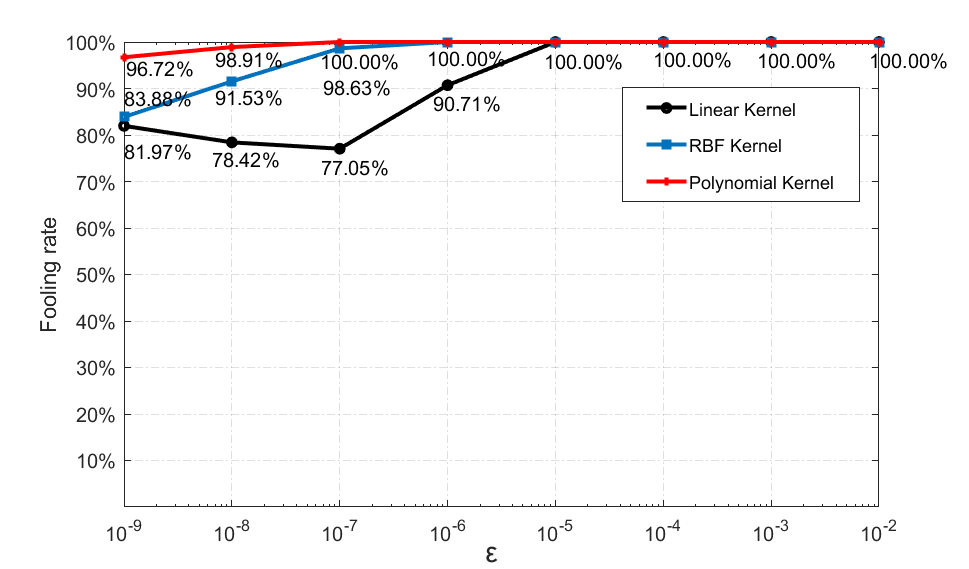
Figure 1: The fooling rate for kernel SVMs with variation of $\varepsilon$.

IV-B2 $\gamma$ in RBF Kernel

To see the role of $\gamma$ in RBF kernel, we conduct some further test with dataset number 1 and number 8. $\gamma$ is chosen from the set $\Gamma=\{0.00001,0.0001,0.001,0.01,0.05,0.09\}$, then we can get six classifiers. We select a fixed data of number 1 and a fixed data of number 8 as the original clean data of positive and negative classes respectively, and we show them at the top of Fig. 2. Then we solve the nonlinear equations system (24), and calculate sAP corresponding to the SVM model when $\gamma\in\Gamma$, and show them in Fig. 2.

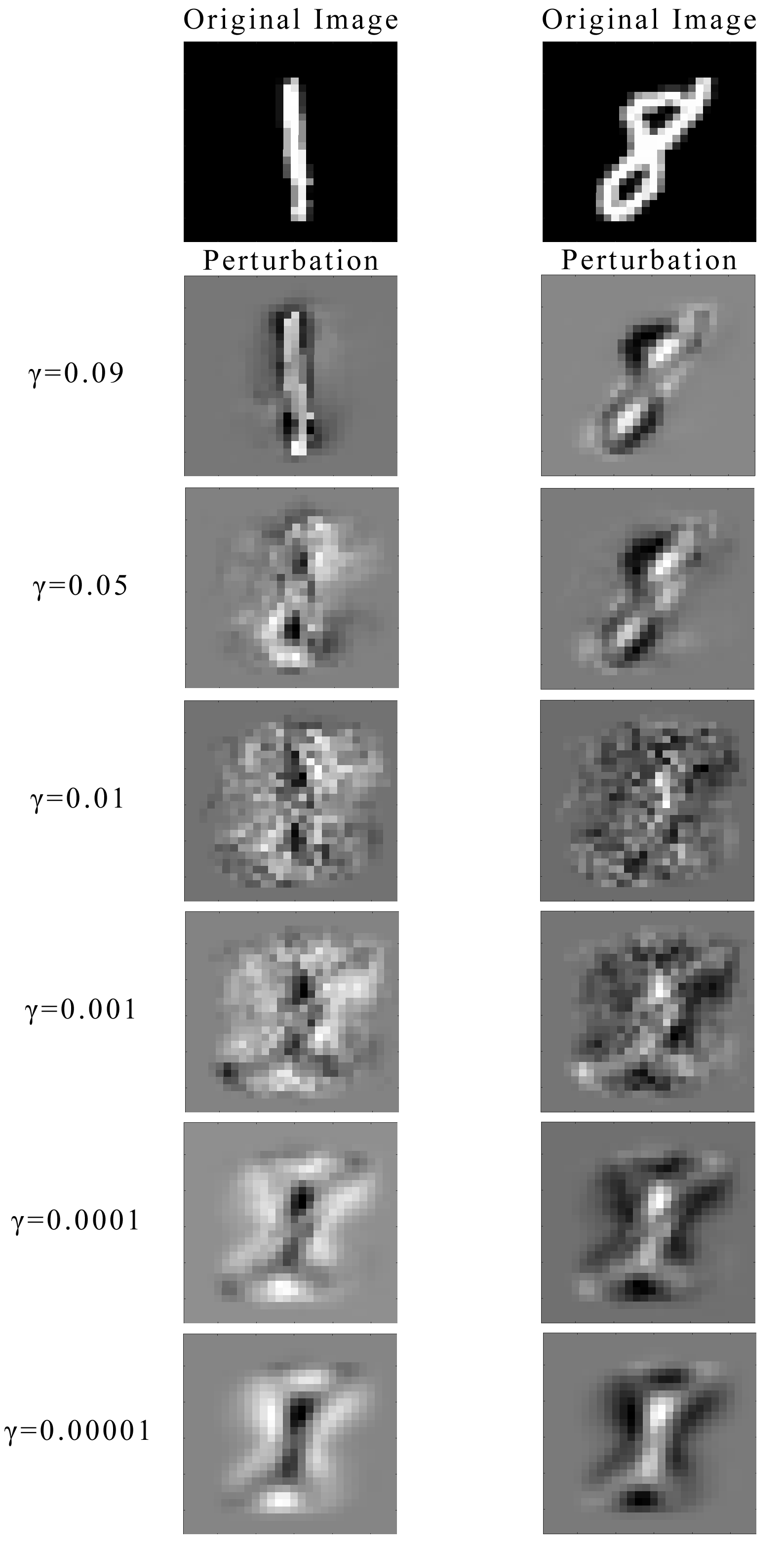
Figure 2: Comparison of adversarial perturbations between positive and negative classes when $\gamma$ changes.

As shown in Fig. 2, after adding the pertubations, the corresponding images’ classes become 8 and 1. We found that even if the range of $\gamma$ is large, our methods have solutions, which means we can get the corresponding attacks, to make the classifier be fooled successfully. At the same time, with the increase of $\gamma$, the obtained sAP gradually approaches the shape of the number itself. When the $\gamma$ is the same, comparing the positive and negative classes horizontally, we find that the adversarial perturbations generated by the positive and negative classes have more properties of themselves and less properties of the other.

IV-B3 $b$ and $p$ in Polynomial Kernel

To see the role of parameters $b$ and $p$ in the polynomial kernel, we conduct further test with dataset number 1 and number 8. We select a fixed number 8 as the original clean image and put it in the upper left of Fig. 3. As we all know, $b$ and $p$ of polynomial kernel determine its nonlinearity. As the default setting in LIBSVM, we fix parameter $a$ as 0. Then we select $b$ from $\{1,4,7,10\}$, and select $p$ from $\{0.01,0.1,1\}$. The adversarial perturbations corresponding to different combinations of $b$ and $p$ are demonstrated in Fig. 3.

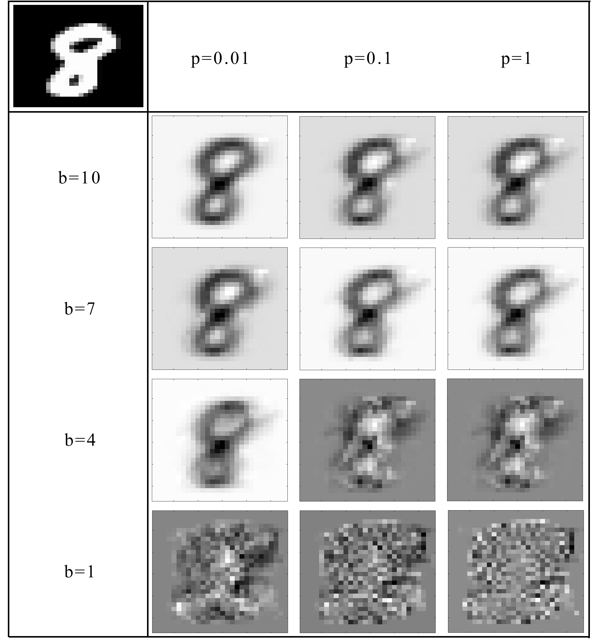
Figure 3: For different $b$ and $p$, the change of adversarial perturbations of the same number 8.

As shown in Fig. 3, when $p$ is fixed, the adversarial perturbations is closer to the original image with the increase of $b$. When $b$ is fixed, with the decrease of $p$, the adversarial perturbations is closer to the original image. It can be seen from Fig. 3 that both $b$ and $p$ have an impact on the adversarial perturbations, and $b$ has a greater impact.

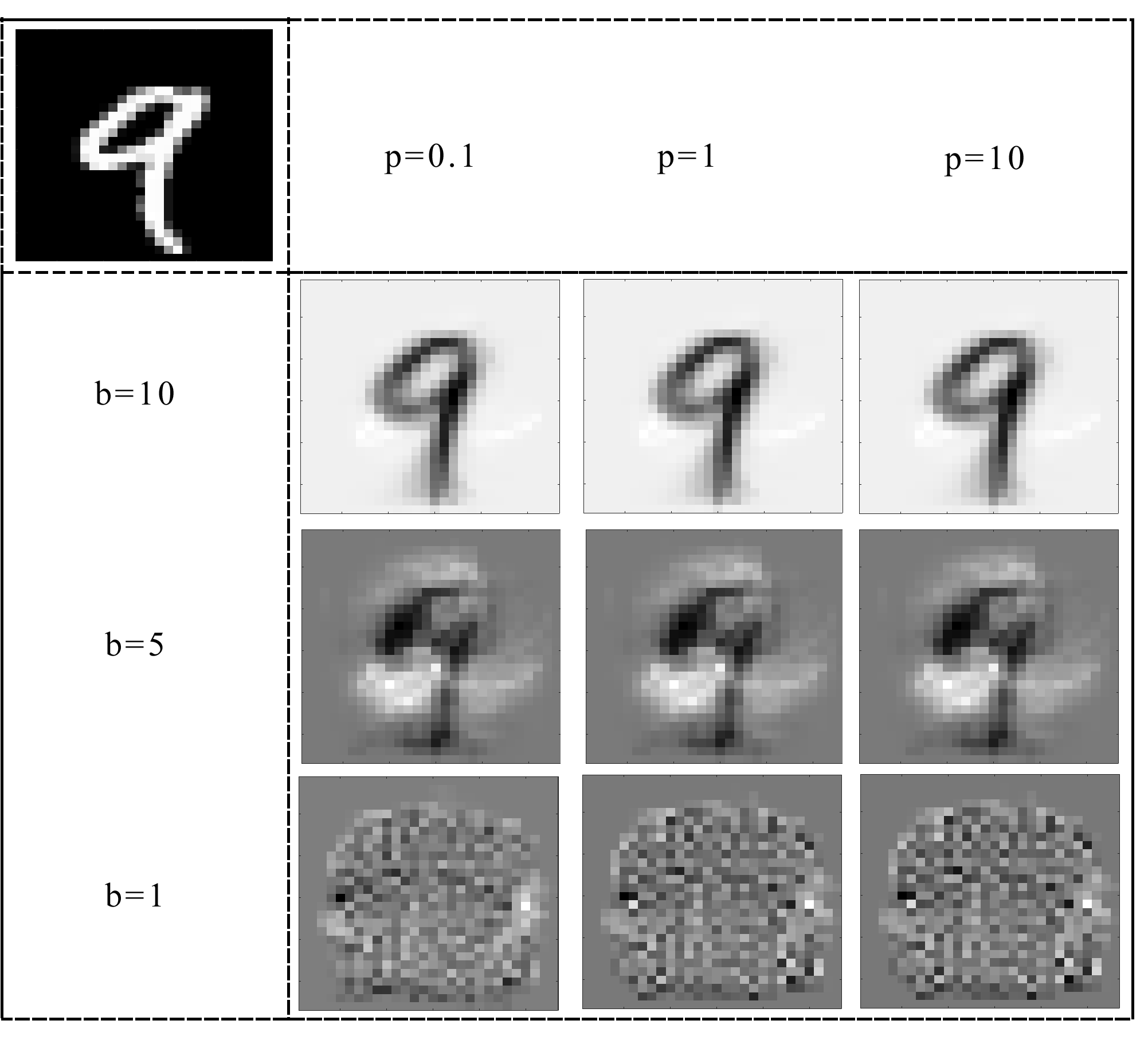
Figure 4: For different $b$ and $p$, the change of adversarial perturbations of the same number 9.

A similar test is conducted with dataset number 2 and number 9, with $a=0$, $b\in\{1,5,10\}$ and $p\in\{0.1,1,10\}$. The result is reported in Fig. 4. It can be seen that when $p$ is fixed, the adversarial perturbations is closer to the original image with the increase of $b$. When $b$ is fixed, the change of $p$ has little effect on the adversarial perturbations.

IV-C Comparison of Methods for linear kernel SVM

In [24], we give the explicit formulae of sAP, uAP and cuAP for linear SVM. In Fig. 5 and Fig. 6, we use the explicit calculation in [24] (short for EC) and Algorithm 2 to solve sAP respectively. In Fig. 5, we give two examples to compare the original image, the image misclassified after being attacked, and the image of sAP of MNIST dataset. At the top of Fig. 5, the original number of the image is 1. After adding the attacks obtained by two methods respectively, the number of the perturbed image becomes 0. Obviously, the attacks obtained by the two methods are the same, and in human eyes, the class of the perturbed images does not change. At the bottom of Fig. 5, the original number of the image is 0. After adding the attacks obtained by the two methods respectively, the number of the perturbed image becomes 1.

Similarly, at the top of Fig. 6, the original image is dog. After adding the attack, the perturbed image becomes truck. At the bottom of Fig. 6, the original image is truck and the perturbed image is dog.

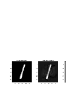
(a) Results by EC method.

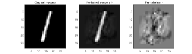
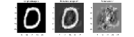
(b) Results by Algorithm 2.

Figure 5: The original image, the image that has been misclassified after being attacked, and the image of sAP against linear kernel SVM.

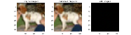
(a) Results by EC method.

(b) Results by Algorithm 2.

Figure 6: The original image, the image that has been misclassified after being attacked, and the image of sAP against linear kernel SVM.

IV-D Numerical experiments of CIFAR-10

For CIFAR-10, we conduct experiment on the most widely RBF kernel SVM, with $\gamma=0.001$. We selected dog in the dataset for the positive classes and truck for the negative classes, a total of 4038. We calculate the change of the fooling rate of adversarial perturbations for data with the change of $\varepsilon$. Fig. 7 shows our results. In the case of RBF kernel, the fooling rate increases with the increase of $\varepsilon$. When $\varepsilon$ is greater than $10^{-5}$, the fooling rate can reach $100\%$. In the following experiments, we choose $\varepsilon=10^{-5}$.

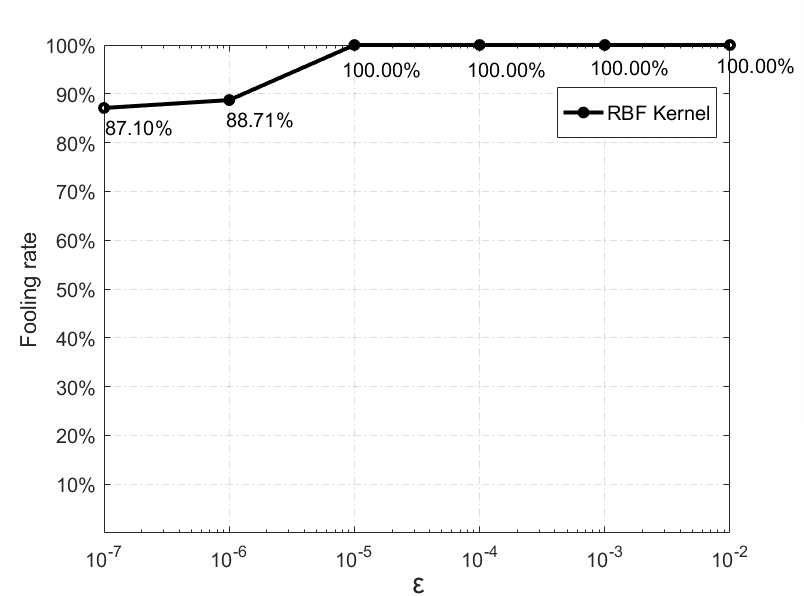
Figure 7: The fooling rate for RBF kernel SVM with variation of $\varepsilon$.

In Fig. 8, we select dog and truck, airplane and frog, automobile and bird, horse and cat as positive and negative classes pairs respectively, to build RBF kernel SVMs, and then solve the corresponding adversarial perturbations respectively. As shown in Fig. 8, the first column are the original images, the second are the images after adding the attacks, and the third are the adversarial perturbations. We marked the classes of each image directly below the images. Through comparison, we find that the images after adding the attacks are basically the same as the original images in the human eyes, but the classes of the images after adding the attacks are actually opposite to the original images.

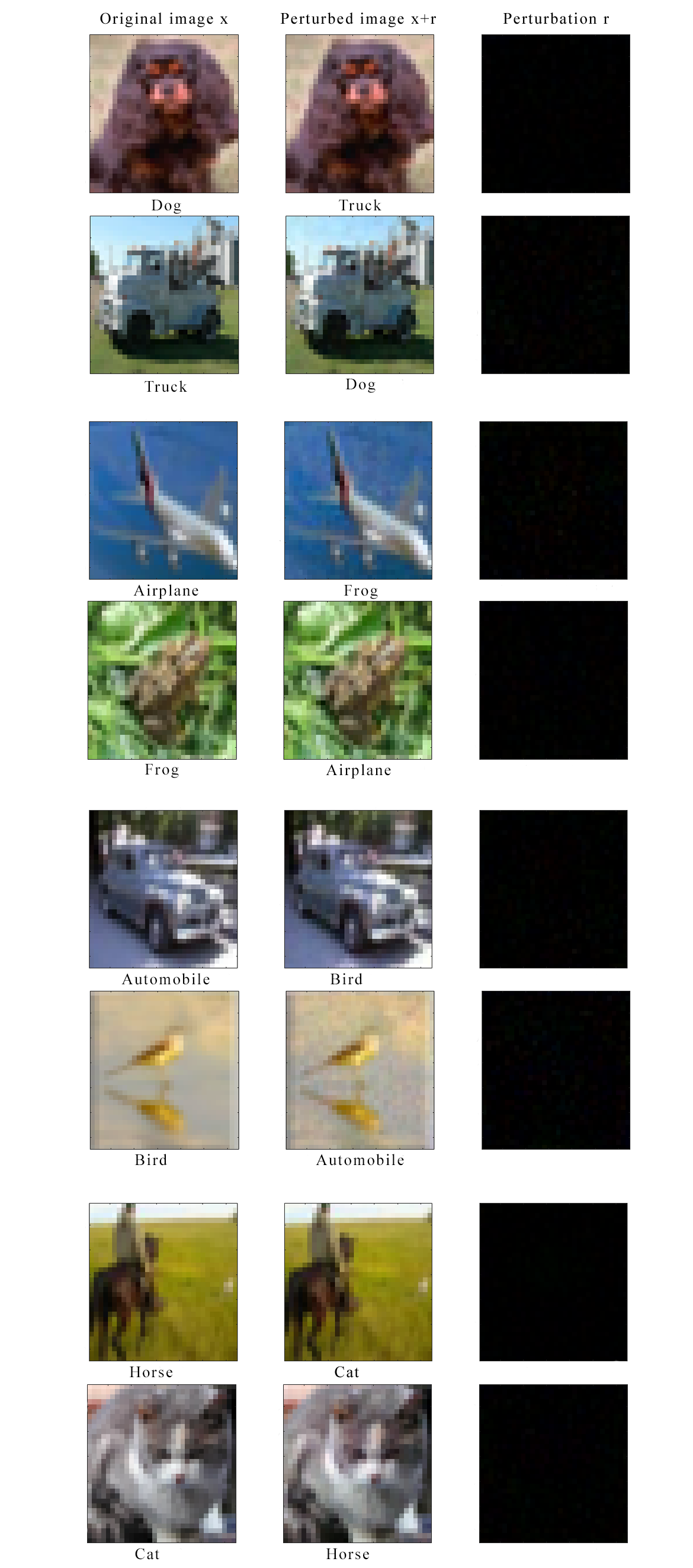
Figure 8: The original images, the images that have been misclassified after being attacked, and the images of sAP against RBF kernel SVM.

V Conclusions

In this paper, we study the problem of adversarial perturbations for kernel SVMs. In the past papers, the research on adversarial perturbation of machine learning models (especially nonlinear models) is basically generated based on a large number of iterative processes or approximate methods. These methods not only have a long iterative process, but also the attack is imprecise. At the same time, the researches on adversarial perturbations have been focused on simple generation, and it is difficult to find the essential relationship between attack and model. In this paper, we transform the original nonlinear optimization problem into a nonlinear KKT system, which avoids the difficulties of the corresponding optimization problem and obtains effective and accurate results. In the numerical experiment part, we give the effective results of linear kernel, RBF kernel and polynomial kernel SVMs respectively. At the same time, it is observed from our visual experiment that the changes of parameters of RBF kernel and polynomial kernel will produce attacks with great differences. In summary, on the one hand, accurate solution makes our method superior to other advanced methods in calculating adversarial perturbations (the fooling rate of our method can reach $100\%$). Further, accurate attack can avoid our operation from being found to the greatest extent, because it is the smallest attack vector compared with other methods. At this time, the small attack can be applied to the environment with practical significance when human cannot observe. On the other hand, we also provide some insights into the influence of the parameters in the SVMs on the adversarial perturbation, such as the relationship between the generated attacks and the linearity of the models, and the relationship between the parameters in the nonlinear models. In addition, based on our method, more research on improving the parameters of the model to enhance the robustness of the model to attacks can be carried out in the future.

References

- [1] M. Guo, T. Xu, J. Liu, Z. Liu, P. Jiang, T. Mu, S. Zhang, R. Martin, M. Cheng and S. Hu, “Attention mechanisms in computer vision: A survey,” Computational visual media, vol. 8, pp. 331–368, 2022.
- [2] A. Esteva, K. Chou, S. Yeung, N. Naik, A. Madani, A. Mottaghi, Y. Liu, E. Topol, J. Dean and R. Socher , “Deep learning-enabled medical computer vision,” npj digital medicine, vol. 4, pp. 5, 2021.
- [3] T. Young, D. Hazarika, S. Poria and E. Cambria, “Recent trends in deep learning based natural language processing,” IEEE computational intelligence magazine, vol. 13, no 3, pp. 55–75, 2018.
- [4] T. Wolf, L. Debut, V. Sanh, J. Chaumond, C. Delangue, A. Moi, et al., “Transformers: state-of-the-art natural language processing,” Proceedings of the 2020 conference on empirical methods in natural language processing: system demonstrations, pp. 38–45, 2020.
- [5] D. Maulud, S. Zeebaree, K. Jacksi, M. Sadeeq and K. Sharif, “State of art for semantic analysis of natural language processing,” Qubahan academic journal, vol. 1, pp. 21–28, 2021.
- [6] Q. Shambour, “A deep learning based algorithm for multi-criteria recommender systems,” Knowledge-based systems, pp. 211, 2021.
- [7] G. Gupta and R. Katarya, “A study of deep reinforcement learning based recommender systems,” 2021 2nd International conference on secure cyber computing and communications (ICSCCC), pp. 218–220, 2021.
- [8] N. Thakur and C. Han, “A Study of Fall Detection in Assisted Living: Identifying and Improving the Optimal Machine Learning Method,” Journal of sensor and actuator networks, vol. 10, pp. 39, 2021.
- [9] N. Thakur and C. Han, “An ambient intelligence-based human behavior monitoring framework for ubiquitous environments,” Information, vol. 12, pp. 81, 2021.
- [10] N. Akhtar and A Mian, “Threat of adversarial attacks on deep learning in computer vision: A survey,” IEEE Access, vol. 3, pp. 14410–14430, 2018.
- [11] C. Szegedy, W. Zaremba, I. Sutskever, J. Bruna, D. Erhan, I. Goodfellow and R. Fergus, “Intriguing properties of neural networks,” https://arxiv.org/abs/1312.6199, 2014.
- [12] I. J. Goodfellow, J. Shlens and C. Szegedy, “Explaining and harnessing adversarial examples,” arXiv preprint arXiv: 1412.6572, 2015.
- [13] T. Miyato, S.I. Maeda, M. Koyama and S. Ishii, “Virtual adversarial training: a regularization method for supervised and semi-supervised learning,” IEEE transactions on pattern analysis and machine intelligence, vol. 41, no 8, pp. 1979–1993, 2018.
- [14] A. Kurakin, I. J. Goodfellow and S. Bengio, “Adversarial machine learning at scale,” arXiv preprint arXiv: 1611.01236, 2016.
- [15] S. M. Moosavi-Dezfooli, A. Fawzi and P. Frossard, “Deepfool: a simple and accurate method to fool deep neural networks,” Proceedings of the IEEE conference on computer vision and pattern recognition, pp. 2574–2582, 2016.
- [16] J. Su, D. V. Vargas and S. Kouichi, “One pixel attack for fooling deep neural networks,” IEEE Transactions on Evolutionary Computation, vol. 23, no. 5, pp. 828–841, 2017.
- [17] S. M. Moosavi-Dezfooli, A. Fawzi, O. Fawzi and P. Frossard, “Universal adversarial perturbations,” Proceedings of the IEEE conference on computer vision and pattern recognition, pp. 1765–1773, 2017.
- [18] K. R. Mopuri, U. Ojha, U. Garg and R. V. Babu, “Nag: Network for adversary generation,” Proceedings of the IEEE conference on computer vision and pattern recognition, pp. 742–751, 2018.
- [19] K. R. Mopuri, U. Garg and R. V. Babu, “Fast feature fool: A data independent approach to universal adversarial perturbations,” arXiv preprint arXiv: 1707.05572, 2017.
- [20] V. Khrulkov and I. Oseledets, “Art of singular vectors and universal adversarial perturbations,” Proceedings of the IEEE Conference on Computer Vision and Pattern Recognition, pp. 8562–8570, 2018.
- [21] C. Zhang, P. Benz, T. Imtiaz and I. S. Kweon. “CD-UAP: Class discriminative universal adversarial perturbation,” Proceedings of the AAAI conference on artificial intelligence, vol. 34, no. 04, pp. 6754–6761, 2020.
- [22] A. Fawzi, O. Fawzi and P. Frossard, “Analysis of classifiers’ robustness to adversarial perturbations,” Machine learning, vol. 107, no. 3, pp. 481–508, 2018.
- [23] P. Langenberg, E. Balda, A. Behboodi and R. Mathar, “On the robustness of support vector machines against adversarial examples,” 13th international conference on signal processing and communication systems (ICSPCS), pp.1–6, 2019.
- [24] W. Su, Q. Li and C. Cui, “Optimization models and interpretations for three types of adversarial perturbations against support vector machines,” arXiv preprint arXiv: 2204.03154, 2022.
- [25] Y. LeCun, L. Bottou, Y. Bengio and P. Haffner, “Gradient-based learning applied to document recognition,” Proceedings of the IEEE, vol. 86, no. 11, pp. 2278–2324, 1998.
- [26] A. Krizhevsky, “Learning multiple layers of features from tiny images,” 2009.