Plane polynomials and Hamiltonian vector fields
determined by their singular points

Abstract

Let $\Sigma(f)$ be critical points of a polynomial $f\in\mathbb{K}[x,y]$ in the plane $\mathbb{K}^{2}$, where $\mathbb{K}$ is $\mathbb{R}$ or $\mathbb{C}$. Our goal is to study the critical point map $\mathfrak{S}_{d}$, by sending polynomials $f$ of degree $d$ to their critical points $\Sigma(f)$. Very roughly speaking, a polynomial $f$ is essentially determined when any other $g$ sharing the critical points of $f$ satisfies that $f=\lambda g$; here both are polynomials of at most degree $d$, $\lambda\in\mathbb{K}^{*}$. In order to describe the degree $d$ essentially determined polynomials, a computation of the required number of isolated critical points $\delta(d)$ is provided. A dichotomy appears for the values of $\delta(d)$; depending on a certain parity the space of essentially determined polynomials is an open or closed Zariski set. We compute the map $\mathfrak{S}_{3}$, describing under what conditions a configuration of four points leads to a degree three essentially determined polynomial. Furthermore, we describe explicitly configurations supporting degree three non essential determined polynomials. The quotient space of essentially determined polynomials of degree three up to the action of the affine group $\hbox{\it Aff}\hskip 1.42271pt(\mathbb{K}^{2})$ determines a singular surface over $\mathbb{K}$.

MSC: 35B45; 35R09; 35B65; 35B33

Keywords: Real and complex plane polynomials, Hamiltonian vector fields, singular critical points

1 Introduction

Let $\mathbb{K}=\mathbb{R}$ or $\mathbb{C}$. We then ask under what conditions a polynomial $f\in\mathbb{K}[x,y]$ is essentially determined by its critical points $\Sigma(f)\subset\mathbb{K}^{2}$? Thus, we want to study the critical point map sending polynomials of degree $d$ to their critical points

$$\mathfrak{S}_{d}:f\longmapsto\Sigma(f)\,,$$ (1)

where $\Sigma(f)\doteq I(f_{x},f_{y})$ is the affine algebraic variety (not necessarily reduced) generated by the ideal of partial derivatives of $f$, see Definition 7. Our approximation route uses a finite dimensional framework. Let $\mathbb{K}[x,y]^{0}_{\leq d}$ be the $\mathbb{K}$–vector space of polynomials having at most degree $d$ ($\geq 3$) and zero independent term, and let $\mathcal{P}=\{(x_{\iota},y_{\iota})\}$ be a configuration of $n$ different points in the plane. The linear projective subspace of the polynomials with critical points at least in $\mathcal{P}$, denoted as

$$\mathcal{L}_{d}(\mathcal{P})\doteq Proj\big{(}\{f\in\mathbb{K}[x,y]^{0}_{\leq d}\ |\ \mathcal{P}\subseteq\Sigma(f)\}\big{)},$$ (2)

is well defined. We say that a polynomial $f$ is essentially determined by $\mathcal{P}$ when $\mathcal{L}_{d}(\mathcal{P})$ is a projective point $\{\lambda f\ |\ \lambda\in\mathbb{K}^{*}\}$, see Definition 4. All this leads us to the following.

Interpolation problem for critical points. Let $\mathcal{P}\subset\mathbb{K}^{2}$ be a configuration of $n$ different points, we try to determine the projective subspace $\mathcal{L}_{d}(\mathcal{P})$ of polynomials of at most degree $d$ with critical points at least in $\mathcal{P}$.

This problem has several novel features. The critical values $\{c_{\iota}\}\subset\mathbb{K}$ of $f$ can appear in different level curves $\{f(x,y)-c_{\iota}=0\}$; it is natural in Hamiltonian vector field theory and moduli spaces of polynomials, see P. G. Wightwick [18] and J. Fernández de Bobadilla [11]. This is a main difference with the widely considered problem of linear system of curves in $\mathbb{CP}^{2}$, e.g. R. Miranda, [15] and C. Ciliberto [8].

Very roughly speaking, for degree $d\geq 3$ the relevant data are the cardinality and position of the configuration $\mathcal{P}$, as candidate to be a critical point configuration $\Sigma(f)$. For degree three, the prescription of four critical points is suitable. For degree $d\geq 4$, however, the generic configuration $\mathcal{P}$ having $(d-1)^{2}$ points is too restrictive. Thus the fiber $\mathfrak{S}_{d}^{-1}(\mathcal{P})$ will be generically empty. It follows that, the position of the configurations $\mathcal{P}$ coming from polynomials is the hardest part to be characterized. At this first stage, we consider mainly $\mathcal{P}$ as isolated points of multiplicity one, Remark 1 provides an explanation. Our first result describes the role of cardinality $\delta(d)$ of $\mathcal{P}$ in Eq. (2), see Proposition 1.

Dichotomy on the required number of critical points

If the dimension of $\mathbb{K}[x,y]^{0}_{\leq d}$ is odd (resp. even) then the configurations $\{\mathcal{P}\}$ with $\delta(d)$ points and $dim_{\mathbb{K}}(\mathcal{L}_{d}(\mathcal{P}))\geq 0$ determine an open (resp. closed) Zariski set in the space of configurations with $\delta(d)$ points, denoted as ${\it Conf}(\mathbb{K}^{2},\delta(d))$.

We compute the critical point map $\mathfrak{S}_{3}$. Thus, a description for the four critical point configurations $\{\mathcal{P}\}$ with essentially determined polynomials is provided. Recall that the affine group $\hbox{\it Aff}\hskip 1.42271pt(\mathbb{K}^{2})$ acts on the space of polynomials, see Eq. (20). This action is rich enough and yet treatable for degree three. Let

$\mathscr{A}\doteq\{x_{4}y_{4}(x_{4}+y_{4}-1)(x_{4}+y_{4})(x_{4}-1)(y_{4}-1)=0\}\subset\mathbb{K}^{2}=\{(x_{4},y_{4})\}$

be an arrangement of six lines from two nested triangles, one of them is $\triangle=\{(0,0),(1,0),(0,1)\}$; see Fig. 1.a. We prove the following result.

Theorem 1.

Let $f$ be a degree three polynomial having at least four critical points $\Sigma(f)$.

1. $f$ is essentially determined if and only if up to affine transformation the four points are

   $$\Sigma(f)=\{(0,0),(1,0),(0,1),(x_{4},y_{4})\}\hbox{\ and \ }(x_{4},y_{4})\notin\mathscr{A}.$$

2. $f$ is not essentially determined if and only if up to affine transformation the four points are

   $$\{(0,0),(1,0),(0,1),(x_{4},y_{4})\}\hbox{\ and \ }(x_{4},y_{4})\in\mathscr{A}.$$

   Moreover, in this case $\Sigma(f)$ can be four isolated points or two parallel lines.

In simple words, the 4–th point $(x_{4},y_{4})$ generically determines the polynomial $f$. We compute the fundamental domain for this $\hbox{\it Aff}\hskip 1.42271pt(\mathbb{K}^{2})$–action, obtaining a tessellation of $\mathbb{K}^{2}=\{(x_{4},y_{4})\}$ with 24 tiles, a seen in Fig. 3.

As is expected, some interesting phenomena occur for configurations with non trivial isotropy groups. For degree $d\geq 3$, a particular family of configurations is the grids of $(d-1)^{2}$ points from the intersection of two families of $d$ parallel lines in $\mathbb{K}^{2}$, see Definition 8. They provide examples of non essential determined polynomials with $(d-1)^{2}$ Morse critical points. A remaining open question, are these grids of $(d-1)^{2}$ points the unique mechanism in order to produce non essential determined Morse polynomials?

From the point of view of vector fields, we are studying under what conditions the zeros a Hamiltonian vector field determine it in a unique way? This is a very general and interesting issue in real and complex foliation theory, studied by; X. Gómez–Mont, G. Kempf [13], J. Artes, J. Llibre, N. Vulpe [4], A. Campillo, J. Olivares [6] and V. Ramírez [17] see Corollary 5. Related works are accurately described in Section §7.

The content of this work is as follows. In §2–3, we study the problem of the dimension of linear systems for polynomials with critical points, using the degree as parameter. In section §4, we characterize polynomials essentially determined by their configurations of critical points; this proves Theorem 1. In section §5, we focus in the degree four case. For each configuration of six points, we obtain a plane curve of degree six parametrizing the essentially determined polynomials, see Proposition 2. Section §6 explores the behavior of pencils of Hamiltonian vector fields with common simple zeros.

2 Linear systems $\mathcal{L}_{d}(\mathcal{P})$

Let $\mathbb{K}[x,y]^{0}_{\leq d}$ (resp. $\mathbb{K}[x,y]^{0}_{=d}$) be the $\mathbb{K}$–vector space of polynomials having at most degree $d\geq 3$ (resp. the set for degree $=d$) and zero independent term. Consider

$$f(x,y)=\sum_{1\leq\iota+j\leq d}a_{\iota j}x^{\iota}y^{j}\ \ \in\mathbb{K}[x,y]_{\leq d}^{0},$$ (3)

from which the $\mathbb{K}$–dimension of $\mathbb{K}[x,y]_{\leq d}^{0}$ is $\frac{1}{2}(d^{2}+3d)$, and its projectivization is

$$Proj\big{(}\mathbb{K}[x,y]^{0}_{\leq d}\big{)}=\big{\{}[f]\ |\ f\in\mathbb{K}[x,y]^{0}_{\leq d}\big{\}}=\mathbb{K}\mathbb{P}^{\frac{1}{2}(d^{2}+3d-2)},$$ (4)

where $[\ \ ]$ denotes a projective class. Recall that

$${\it Conf}(\mathbb{K}^{2},n)=\big{\{}\,\mathcal{P}=\{(x_{1},y_{1}),\ldots,(x_{n},y_{n})\}\ |\ (x_{\iota},y_{\iota})\neq(x_{j},y_{j})\hbox{ for }\iota\neq j\big{\}}/Sym(n)$$ (5)

is the space of unordered configurations of $n$ points in $\mathbb{K}^{2}$, where the symmetric group in $n$ elements, $Sym(n)$, acts by exchanging the points. The configuration space ${\it Conf}(\mathbb{K}^{2},n)$ is a $\mathbb{K}$–analytic manifold.

Definition 1.

Given a configuration $\mathcal{P}\in{\it Conf}(\mathbb{K}^{2},n),$ the linear system of polynomials of at most degree $d$ with critical points at least in $\mathcal{P}$ is the projective subspace

$$\mathcal{L}_{d}(\mathcal{P})=\big{\{}[f]\ |\ \mathcal{P}\subseteq\{f_{x}(x,y)=0\}\cap\{f_{y}(x,y)=0\}\big{\}}\subset Proj\big{(}\mathbb{K}[x,y]^{0}_{\leq d}\big{)}.$$ (6)

In algebraic geometry language, $\{f_{x}(x,y)=0\}$, $\{f_{y}(x,y)=0\}$ belong to the linear system of algebraic curves

$\mathcal{L}_{d-1}\big{(}-\Sigma_{\alpha=1}^{n}(x_{\iota},y_{\iota})\big{)}$

see [15] and [8]. In several places however, we consider $f_{x}$, $f_{y}$ as functions and not just as algebraic curves.

The polynomials of at most degree $d$, the polynomial Hamiltonian vector fields and the polynomial vector fields, of at most degree $d-1$, are related by linear maps

$$\begin{array}[]{ccccc}\mathbb{K}[x,y]^{0}_{\leq d}&\stackrel{{\scriptstyle\cong}}{{\longleftrightarrow}}&Ham(\mathbb{K}^{2})_{\leq d-1}&\longrightarrow&\mathfrak{X}(\mathbb{K}^{2})_{\leq d-1}\\ &&&&\vspace{-.3cm}\hfil\\ f&\longleftrightarrow&X_{f}=-f_{y}\frac{\partial}{\partial x}+f_{x}\frac{\partial}{\partial y}&\longrightarrow&X_{f}.\end{array}$$

In the space of Hamiltonian vector fields, $\mathcal{L}_{d}(\mathcal{P})$ determines a linear subspace

$$\{\lambda X_{f}\ |\ \mathcal{P}\subseteq\mathcal{Z}(\lambda X_{f}),\ \lambda\in\mathbb{K}^{*}\}\subset Ham(\mathbb{K}^{2})_{\leq d-1};$$

set theoretically, the zeros $\mathcal{Z}(\lambda X_{f})$ of the vector field $X_{f}$ coincide with $\{f_{x}(x,y)=0\}\cap\{f_{y}(x,y)=0\}$.

Definition 2.

Let $f\in\mathbb{K}[x,y]$ be a non constant polynomial. Over $\mathbb{K}=\mathbb{C}$, the Milnor number of $X_{f}$ at a zero point $(x_{\iota},y_{\iota})\in\mathcal{Z}(X)$ is

$\mu_{(x_{\iota},y_{\iota})}(X)=\dim_{\mathbb{C}}\frac{\mathcal{O}_{\mathbb{C}^{2},(x_{\iota},y_{\iota})}}{<-f_{y},f_{x}>}$,

where $\mathcal{O}_{\mathbb{C}^{2},(x_{\iota},y_{\iota})}$ is the local ring of holomorphic functions at the point $(x_{\iota},y_{\iota})$ and $<-f_{y},f_{x}>$ is the ring generated by the partial derivatives.

Remark 1.

1. Over $\mathbb{K}=\mathbb{C}$, if $(x_{\iota},y_{\iota})$ is an isolated singular point of $f$, then the notions of multiplicity for the intersection of the curves $\{f_{x}(x,y)=0\}\cup\{f_{y}(x,y)=0\}$ and the Milnor number for $X_{f}$ coincide; see [14] p. 174.

2. A priori, we consider each point $(x_{\iota},y_{\iota})\in\mathcal{P}$ in (6) with multiplicity of intersection one for the algebraic curves $\{f_{x}(x,y)=0\}$ and $\{f_{y}(x,y)=0\}$.

3. By Bézout’s theorem, the maximal number of isolated singularities of $X_{f}$ on $\mathbb{C}^{2}$ is $(d-1)^{2}$. In this case all the affine singularities are of multiplicity one.

4. Moreover, the maximal number of isolated singularities of $X_{f}$ extended to $\mathbb{CP}^{2}$ is

$(d-1)^{2}+d$.

Here the upper bound $d$ comes from the intersection of a generic projectivized level curve $\{f=c\}$ with the line at infinity; see [13], [6] for the case of rational vector fields, which are not necessarily Hamiltonian.

Let $\mathbb{A}^{2}_{\mathbb{K}}=\hbox{Spec}\,\mathbb{K}[x,y]$ be the affine scheme of the affine plane $\mathbb{K}^{2}$, see [10] pp. 48–49.

Definition 3.

The critical point map of degree $d$ is the map

$$\begin{array}[]{rcl}\mathfrak{S}_{d}:\mathbb{K}[x,y]_{=d}&\longrightarrow&\hbox{Spec}\,\mathbb{K}[x,y]\\ &&\vspace{-.2cm}\\ f&\longmapsto&\Sigma(f)=I(f_{x},f_{y})\,,\end{array}$$ (7)

sending a polynomial of degree $d$ to its critical points $\Sigma(f)$, as an affine algebraic variety (not necessarily reduced) generated by the ideal of partial derivatives of $f$.

In fact, $\Sigma(f)$ can be understood as a subscheme, with support at the points $\{f_{x}(x,y)=0\}\cap\{f_{y}(x,y)=0\}$, where the sheaf of ideals is defined by the germs of $I(f_{x},f_{y})$; compare with [6], [10] p. 100. In a set theoretical language, $\Sigma(f)$ determines points and even algebraic curves. However in the study of rational vector fields on $\mathbb{CP}^{2}$, the case of foliations having singularities along curves is removed, see [13], [6].

Remark 2.

The simplest case of the interpolation problem for singular points occurs when $\Sigma(f)$ is a finite set of points of multiplicity one, i.e. $\{f_{x}(x,y)=0\}$ and $\{f_{y}(x,y)=0\}$ have transversal intersections. The $\Sigma(f)$ is a configuration in ${\it Conf}(\mathbb{K}^{2},n)$, for $0\leq n\leq(d-1)^{2}$.

Our former task is as follows: Given a configuration $\mathcal{P}$, which is $dim_{\mathbb{K}}(\mathcal{L}_{d}(\mathcal{P}))$?

To be clear, three relevant data must be considered the degree $d$ of the polynomials $\{f\}$, the cardinality $n$ and the position of the configuration $\mathcal{P}$. The following diagram explains:

The natural concepts are as follows.

Definition 4.

Let $f\in\mathbb{K}[x,y]_{\leq d}^{0}$ be a polynomial and let $\mathcal{P}$ be a configuration of $n$ points in $\mathbb{K}^{2}$.

1. A polynomial $f$ is essentially determined by $\mathcal{P}$ when $[f]=\mathcal{L}_{d}(\mathcal{P})$.

2. A polynomial $f$ is non essential determined by $\mathcal{P}$ when $[f]\in\mathcal{L}_{d}(\mathcal{P})$ and $dim_{\mathbb{K}}(\mathcal{L}_{d}(\mathcal{P}))\geq 1$.

3. $\mathcal{P}$ is a forbidden configuration (for polynomials of at most degree $d$) when $\mathcal{L}_{d}(\mathcal{P})=\emptyset$.

4. The set of degree $d$ essentially determined polynomials is

   $$\mathcal{E}_{d}\doteq\bigcup_{\tiny{\mathcal{P}}}\mathcal{L}_{d}(\mathcal{P})\subset Proj\big{(}\mathbb{K}[x,y]^{0}_{\leq d}\big{)},$$ (9)

   where the union is over all configurations $\{\mathcal{P}\}$ such that $dim_{\mathbb{K}}(\mathcal{L}_{d}(\mathcal{P}))=0$.

Remark 3.

1. The strict set theoretical inclusion $\mathcal{P}\varsubsetneq\Sigma(f)$ can be satisfied for essentially determined polynomials $f$, for example as with the case of a product of three lines one with multiplicity two, say $f=L_{1}^{2}L_{2}$.

2. The set of degree three essentially determined polynomials $\mathcal{E}_{3}$ is a union of projective spaces, however it is not a projective space, as Proposition 1 will show.

3. As is expected, many of the projective classes in $\mathcal{E}_{d}$ arise from Morse polynomials. The converse is not true, see Corollary 6.

3 On the number of required critical points

A novel aspect of the interpolation problem for critical points is its cardinality; the configurations having a certain number $\delta(d)$ of points determine open or closed Zariski sets in $\mathbb{K}[x,y]_{\leq d}^{0}$. As a key point, the dimension $\frac{1}{2}(d^{3}+3d)$ of $\mathbb{K}[x,y]_{\leq d}^{0}$ can be even or odd. Starting with degree $d=4$, the pattern of these dimensions is 4–periodic; even, even, odd odd, $\ldots$ . See the third column in Table 1.

Proposition 1.

(A dichotomy on the number $\delta(d)$ of required critical points)  Let $\mathbb{K}[x,y]^{0}_{\leq d}$ be the set of polynomials having at most degree $d\geq 3$ and let

$$\delta(d)\doteq\left\{\begin{array}[]{cl}\frac{1}{4}(d^{2}+3d-2)&\hbox{ when }\frac{1}{2}(d^{2}+3d)\hbox{ is odd},\\ &\vspace{-.2cm}\\ \frac{1}{4}(d^{2}+3d)&\hbox{ when }\frac{1}{2}(d^{2}+3d)\hbox{ is even}.\end{array}\right.$$ (10)

1. If the dimension of $\mathbb{K}[x,y]^{0}_{\leq d}$ is odd, then the configurations $\{\mathcal{P}\}$ with $\delta(d)$ points and $dim_{\mathbb{K}}(\mathcal{L}_{d}(\mathcal{P}))\geq 0$ determine an open Zariski set in ${\it Conf}(\mathbb{K}^{2},\delta(d))$.

2. If the dimension of $\mathbb{K}[x,y]^{0}_{\leq d}$ is even, then the configurations $\{\mathcal{P}\}$ with $\delta(d)$ points and $dim_{\mathbb{K}}(\mathcal{L}_{d}(\mathcal{P}))\geq 0$ determine a closed Zariski set in ${\it Conf}(\mathbb{K}^{2},\delta(d))$.

Proof.

Let $f(x,y)\in\mathbb{K}[x,y]^{0}_{\leq d}$ be a polynomial as in (3). Assume that $\mathcal{P}=\{(x_{\iota},y_{\iota})\ |\ \iota=1,\ldots,n\}$ is set theoretically contained in $\Sigma(f)$. A priori, each point $(x_{\iota},y_{\iota})\in\mathcal{P}$ will drop the dimension of the vector space $\mathbb{K}[x,y]^{0}_{\leq d}$ by two. In the linear framework, this leads to a linear system of $2n$ equations:

$$f_{x}(x_{\iota},y_{\iota})=f_{y}(x_{\iota},y_{\iota})=0,\ \ \ \ \iota=1,\ldots,n,$$ (11)

with $\{a_{\iota j}\}$ as variables. Following Bézout’s theorem for a moment, let us consider a configuration with $n=(d-1)^{2}$ points. We have a linear map

$$\begin{array}[]{rcl}\phi:\mathbb{K}[x,y]^{0}_{\leq d}\cong\mathbb{K}^{\frac{1}{2}(d^{2}+3d)}&\longrightarrow&\mathbb{K}^{2(d-1)^{2}}\\ f&\longmapsto&\big{(}f_{x}(x_{1},y_{1}),\ldots,f_{x}(x_{(d-1)^{2}},y_{(d-1)^{2}}),\,f_{y}(x_{1},y_{1}),\ldots,f_{y}(x_{(d-1)^{2}},y_{(d-1)^{2}})\big{)}.\end{array}$$ (12)

The interpolation matrix $\phi$ depends on $\mathcal{P}$, and by notational simplicity we omit this dependence. The matrix $\phi$ has $\frac{1}{2}(d^{2}+3d)$ columns, $2(d-1)^{2}$ rows and a very particular shape because of the partial derivatives involved in it, see Eqs. (17), (33) for explicit examples with $d=3$, $4$.

For degree $d=3$ and a configuration $\mathcal{P}$ of 4 points; however then the rank of the matrix $\phi$ associated to $\mathcal{P}$ is 8 if and only if $dim_{\mathbb{K}}(\mathcal{L}_{3}(\mathcal{P}))=0$. If we consider degree $d\geq 4$, then the number of rows of $\phi$ is bigger than the number of columns. We must reduce the number $n$ of required points in the configurations $\mathcal{P}$, this $n<(d-1)^{2}$. The number $\delta(d)$ in (10) determines two possibilities.

Case 1 in (10). For $\mathcal{P}$ with $\delta(d)=\frac{1}{4}(d^{2}+3d-2)$ points, the interpolation matrix $\phi$ has $\frac{1}{2}(d^{2}+3d)$ odd columns and $\frac{1}{2}(d^{2}+3d-2)$ even rows, for example for $(d+1)=3,6,7$. Moreover,

(number of columns of $\phi$)–1 = (number of rows of $\phi$).

The dimension of the kernel of $\phi$ is at least one, thus $dim_{K}(\mathcal{L}_{d}(\mathcal{P}))\geq 0$. There are $\frac{1}{2}(d^{2}+3d)$ minors $A_{j}$ from the matrix $\phi(x_{1},y_{1},\ldots,x_{\delta(d)},y_{\delta(d)})$. The complement of the algebraic equations

$\{\Pi_{j}det(A_{j}(x_{1},y_{1},\ldots,x_{\delta(d)},y_{\delta(d)}))=0\}\subset{\it Conf}(\mathbb{K},\delta(d))$

describes the set of configurations having $dim_{K}(\mathcal{L}_{d}(\mathcal{P}))=0$, corresponding to the essentially determined polynomials. These configurations of $\delta(d)$ points in ${\it Conf}_{\delta(d)}(\mathbb{K}^{2})$ determine an open Zariski and dense set, that is the second part of assertion (1).

Case 2 in (10). The dimension of $\mathbb{K}[x,y]_{\leq n}^{0}$ is even and we assume $\frac{1}{4}(d^{2}+3d)\in\mathbb{N}$ points in $\mathcal{P}$. The interpolation matrix $\phi$ is square of even size, and there are $\frac{1}{2}(d^{2}+3d)$ columns and rows; for example when $d=4,5$.

If we assume $\mathcal{P}$ such that $\{det(\phi(x_{1},y_{1},\ldots,x_{\delta(d)},y_{\delta(d)}))\neq 0\}$, then the only vector in the $\{a_{\iota j}\}$ variables solving the linear system (11) is zero. The set of desired polynomials is empty.

The configuration with non empty polynomials

$\left\{\mathcal{P}\ |\ det(\phi(x_{1},y_{1},\ldots,x_{\delta(d)},y_{\delta(d)}))\neq 0\right\}\subset{\it Conf}(\mathbb{K},\delta(d))$

determines an algebraic set. ∎

		number of	number of	Zariski
degree $d$	$\delta(d)$	columns in $\phi$	rows in $\phi$	topology of
	eq. (10)	$\frac{1}{2}(d^{2}+3d)$	$2\delta(d)$	$\{\mathcal{P}\}\subset{\it Conf}(\mathbb{K}^{2},\delta(d))$
3	4	9	8	closed
4	7	14	14	open
5	10	20	20	open
6	13	27	26	closed
7	17	35	34	closed

Table 1: Dimensions and values for the interpolation problem.

Recalling (4), the expected projective dimension of $\mathcal{L}_{d}(\mathcal{P})$, which is the linear system of polynomials of at most degree $d$ with critical points at least in $\mathcal{P}\in{\it Conf}(\mathbb{K}^{2},n)$, is

$max\left\{\frac{1}{2}(d^{2}+3d-2)-2n,\ -1\right\}$.

In Section 5, we provide an alternative for studying the even dimension case in Proposition 1.

4 Essentially determined polynomials of degree three

4.1 A linear system

In order to apply elementary methods, we introduce a very simple configuration of four points, depending essentially of the fourth one $(x_{4},y_{4})$. Secondly, we must find a polynomial $f(x_{4},y_{4},x,y)$ with a critical point set containing the above simple configuration. Let

$$\mathscr{A}\doteq\big{\{}xy(x+y-1)(x+y)(x-1)(y-1)=0\big{\}}$$ (13)

be an arrangement of six $\mathbb{K}$–lines; it is illustrated in Fig. 1.a.

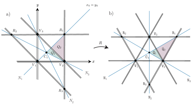
Figure 1: a) The line arrangement $\mathscr{A}$ (of double lines) and the triangle $\triangle=\{V_{1},\,V_{2},\,V_{3}\}$. b) The analogous objects under the linear map $R$, sending $\mathscr{A}$ to ${\tt A}$ and $\triangle$ to $\Delta$.

Lemma 1.

Let

$\mathcal{P}=\{V_{1}=(0,0),\,V_{2}=(1,0),\,V_{3}=(0,1),\,(x_{4},y_{4})\}\in{\it Conf}(\mathbb{K}^{2},4)$,    $(x_{4},y_{4})\notin\mathscr{A}$,

be a four point configuration. The polynomial

$$f(x_{4},y_{4},x,y)= (y_{4}^{2}(y_{4}-1)(-1+2x_{4}+y_{4})(2x^{3}-3x^{2})+x_{4}^{2}(x_{4}-1)(-1+x_{4}+2y_{4})(2y^{3}-3y^{2})$$ (14)

$$- 6x_{4}y_{4}(x_{4}-1)(y_{4}-1)(x^{2}y+xy^{2}-xy))a_{6}\quad\in\mathbb{K}[x,y]_{=3},$$

for $a_{6}\in\mathbb{K}^{*}$, is well defined and $\mathcal{P}=\Sigma\big{(}f(x_{4},y_{4},x,y)\big{)}$.

It shall be convenient to write the Eq. (14) as a map to the space of polynomials

$$f(x_{4},y_{4},\ \ ,\ \ ):\mathbb{K}^{2}\backslash\mathscr{A}\longrightarrow\mathbb{K}[x,y]_{=3},\ \ \ (x_{4},y_{4})\longmapsto f(x_{4},y_{4},x,y).$$ (15)

Proof.

Let the following be a polynomial

$$f(x,y)=a_{1}x^{3}+a_{2}x^{2}y+a_{3}xy^{2}+a_{4}y^{3}+a_{5}x^{2}+a_{6}xy+a_{7}y^{2}+a_{8}x+a_{9}y\ \in\mathbb{K}[x,y]^{0}_{\leq 3}.$$ (16)

By notational simplicity, only one subindex $a_{\iota}$ is considered. Let $\{(x_{\iota},y_{\iota})\ |\ \iota=1,\ldots,4\}$ be an arbitrary configuration, and we require $(a_{1},\ldots,a_{9})$ to be solutions of the linear system

$$\left(\begin{smallmatrix}&&&\vdots&&&&&\\ 3x_{\iota}^{2}&2x_{\iota}y_{\iota}&y_{\iota}^{2}&0&2x_{\iota}&y_{\iota}&0&1&0\\ 0&x_{\iota}^{2}&2x_{\iota}y_{\iota}&3y_{\iota}^{2}&0&x_{\iota}&2y_{\iota}&0&1\\ &&&\vdots&&&&&\end{smallmatrix}\right)\left(\begin{smallmatrix}a_{1}\\ \vdots\\ a_{9}\end{smallmatrix}\right)=\left(\begin{smallmatrix}0\\ \vdots\\ 0\end{smallmatrix}\right).$$ (17)

The interpolation matrix $\phi$ in (17) has 9 columns and 8 rows. The choice $\mathcal{P}=\{(0,0),(1,0),(0,1),(x_{4},y_{4})\}$ determines the linear system with only two equations

$$\begin{array}[]{c}f_{x}(x,y)=3a_{1}x^{2}+2a_{2}xy+a_{3}y^{2}+2a_{5}x+a_{6}y+a_{8}=0,\\ f_{y}(x,y)=a_{2}x^{2}+2a_{3}xy+3a_{4}y^{2}+a_{6}x+2a_{7}y+a_{9}=0.\end{array}$$

Obviously, $(0,0)\in\mathcal{P}$ implies the vanishing of the linear part $f_{x}(0,0)=a_{8}=0=a_{9}=f_{y}(0,0)$. The linear conditions imposed by $(1,0)$ and $(0,1)$ are

$$\left\{\begin{array}[]{lccl}f_{x}(1,0)=3a_{1}+2a_{5}=0&&&a_{1}=-\frac{2}{3}a_{5},\\ f_{y}(1,0)=a_{2}+a_{6}=0&&&a_{6}=-a_{2},\end{array}\right.$$

$$\left\{\begin{array}[]{lccl}f_{x}(0,1)=a_{3}+a_{6}=0&&&a_{6}=-a_{3},\\ f_{y}(0,1)=3a_{4}+2a_{7}=0&&&a_{4}=\frac{-2}{3}a_{7}.\end{array}\right.$$

The solution of this system

$$\begin{array}[]{ll}f(x_{4},y_{4},x,y)=&a_{6}\left(\dfrac{y_{4}(-1+2x_{4}+y_{4})}{3x_{4}(x_{4}-1)}x^{3}-x^{2}y-xy^{2}+\dfrac{x_{4}(-1+x_{4}+2y_{4})}{3y_{4}(y_{4}-1)}y^{3}\right.\\ &\vspace{-.3cm}\\ &\left.\ \ \ \ +\dfrac{y_{4}(1-2x_{4}-y_{4})}{2x_{4}(x_{4}-1)}x^{2}+xy+\dfrac{x_{4}(1-x_{4}-2y_{4})}{2y_{4}(y_{4}-1)}y^{2}\right)\ \ \in\mathbb{K}[x,y]_{=3}\end{array}$$ (18)

has rational coefficients. If we normalize, we get Eq. (14). ∎

Corollary 1.

Let

$\mathcal{P}_{1}=\{(0,0),(1,0),(0,1),R_{1}\doteq(1,1)\}\in{\it Conf}(\mathbb{K}^{2},4)$

be a four point configuration, then $dim_{\mathbb{K}}(Proj(\mathcal{L}_{3}(\mathcal{P}_{1})))=1$.

We say that, $R_{1}=(1,1)$ is a rhombus point; see Fig. 1.

Proof.

By replacing in $\phi$ the points in $\mathcal{P}_{1}$, a direct calculation shows that the equivalent $9\times 8$ matrix has rank 7, where the null space of $\phi$ is given by the vectors $(0,0,0,-2/3,0,0,1,0,0)$ and $(-2/3,0,0,0,1,0,0,0,0)$. The linear combination of the corresponding polynomials leads to

$$f({\tt a,d,}x,y)=a\left(2x^{3}-3x^{2}\right)+d\left(2y^{3}-3y^{2}\right),\ \ \ [a,\,d]\in\mathbb{K}\mathbb{P}^{1}.$$ (19)

∎

Remark 4.

Behavior of the linear system at $\mathscr{A}$. Let $\mathcal{P}=\{(0,0),(1,0),(0,1),(x_{4},y_{4})\}$ be a configuration.

1. If $(x_{4},y_{4})$ tends to be in a line

$L_{\alpha}\subset\mathscr{A}\big{\{}\mathscr{A}\big{\}}\backslash\{R_{1}=(1,1),R_{2}=(-1,1),R_{3}=(1,-1)\},$

then the polynomial $f(x_{4},y_{4},x,y)$ in (17) has two lines of critical points in the respective pair of parallel $\mathbb{K}$–lines $L_{\alpha}$, $L_{\beta}$, in the arrangement $\{\mathscr{A}(x,y)=0\}$. Figure 4 provides a sketch up to affine transformations.

2. If $(x_{4},y_{4})$ tends to be the vertex $(0,0)\in\triangle$, then the polynomial $f(x_{4},y_{4},x,y)$ in (16) becomes

$f(0,0,x,y)=\frac{1}{3}(x^{3}+y^{3})-(x^{2}y+xy^{2})-\frac{1}{2}(x^{2}+y^{2})+xy$.

As is expected, the curve $\{f(0,0,x,y)=0\}$ has a cusp of multiplicity two at (0,0), see Fig. 4. The same is valid if $(x_{4},y_{4})$ tends to be any other vertex $(1,0)$, $(0,1)$ of $\triangle$. Figure 4 shows $f(1,0,x,y)$, corresponding to $V_{2}=(0,1)$ denoted as ${\tt V}_{2}$ in the figure.

Remark 5.

Let $\mathcal{P}$ be any configuration of four points. Thus $\mathcal{L}_{3}(\mathcal{P})\neq\emptyset$, i.e. there exists a non constant degree three polynomial having critical points at least in $\mathcal{P}$.

4.2 Affine classification of quadrilateral configurations

We now study the independence of the previous results §4.1, with respect to the coordinate system.

A valuable tool in the study of polynomials of degree three is the action of the group of affine automorphisms of $\mathbb{K}^{2}$, say $\hbox{\it Aff}\hskip 1.42271pt(\mathbb{K}^{2})$. It is a six $\mathbb{K}$–dimensional Lie group. Let $\hbox{\it Aff}\hskip 1.42271pt(\mathbb{K}^{2})$ acts on the space of polynomials of degree $d$ as

$$\hbox{\it Aff}\hskip 1.42271pt(\mathbb{K}^{2})\times\mathbb{K}[x,y]_{=d}\longrightarrow\mathbb{K}[x,y]_{=d},\ \ \ (T,f)\longmapsto f\circ T.$$ (20)

This action is rich enough and yet treatable. The affine group acts on configurations such as

$$\hbox{\it Aff}\hskip 1.42271pt(\mathbb{K}^{2})\times{\it Conf}(\mathbb{K}^{2},n)\longrightarrow{\it Conf}(\mathbb{K}^{2},n),\ \ \ (T,\mathcal{P})\longmapsto T^{-1}(\mathcal{P}).$$ (21)

Thus, if $f\in\mathbb{K}[x,y]_{=d}$ has $n$ isolated critical points, say $\mathcal{P}\in{\it Conf}(\mathbb{K}^{2},n)$, then $f\circ T$ has critical points at $T^{-1}(\mathcal{P})$. Hence, a useful associated object is the quotient space of quadrilateral configurations up to affine transformations.

Definition 5.

The space of generic quadrilateral configurations is

$$\mathcal{Q}=\left\{\mathcal{P}_{0}=\{(x_{1\,0},y_{1\,0}),\ldots,(x_{4\,0},y_{4\,0})\}\ \Big{|}\ \begin{array}[]{l}\hbox{quadrilaterals configurations}\\ \hbox{having no three collinear vertices }\\ \hbox{or determining two parallel lines}\end{array}\right\}\subsetneq{\it Conf}(\mathbb{K}^{2},4).$$ (22)

Note that a quadrilateral configuration $\mathcal{P}_{0}$ does not have order. It determines several quadrilaterals, i.e. with a cyclic order in its vertices. Let

$$\triangle=\{V_{1}=(0,0),V_{2}=(1,0),V_{3}=(0,1)\},\ \ \ \Delta=\{{\tt V}_{1}=(0,0),{\tt V}_{2}=(1,0),{\tt V}_{3}=(1/2,\sqrt{3}/2)\}$$

be two triangles. Consider a linear transformation $R\in GL(2,\mathbb{K})$ such that $R(\triangle)=\Delta$, $R(V_{2})={\tt V}_{2}$ and $R(V_{3})={\tt V_{3}}$, see Fig. 1. The affine symmetries of $\Delta$,

$$Sym(3)=\{\sigma_{\alpha}\in\hbox{\it Aff}\hskip 1.42271pt(\mathbb{K}^{2})\ |\ \sigma_{\alpha}(\Delta)=\Delta,\ \alpha\in 1,\ldots,6\},$$ (23)

are isomorphic to the symmetric group of order 3; with three reflections $\sigma_{2},\sigma_{4},\sigma_{6}$ (with axis in the lines ${\tt N}_{1},\,{\tt N}_{2},\,{\tt N}_{3}$) and their products $\sigma_{1}=id,\sigma_{3},\sigma_{5}$; see Fig. 1.b. By abusing the notation, $Sym(3)$ also denotes the affine symmetries of $\triangle$.

Thus, we use three coordinate systems as follows. Let $\mathcal{P}_{0}=\{(x_{1\,0},y_{1\,0}),\ldots,(x_{4\,0},y_{4\,0})\}$ as in (22). By using the affine action, we reduce $\mathcal{P}_{0}$ to $\{(x_{4},y_{4})\}$ or $\{({\tt x}_{4},{\tt y}_{4})\}$. There are affine maps $T_{j}\in\hbox{\it Aff}\hskip 1.42271pt(\mathbb{K}^{2})$,

(24)

By notational simplicity, we also denote by $\mathcal{P}$ the configuration on the right side.

A key point is the number of affine maps $\{T_{j}\}$, depending on $\mathcal{P}_{0}$ to be computed in Corollary 2.

In accordance with Fig. 1 and 3, the triangles $\triangle$, $\Delta$ determine the points, line arrangements and regions below.

$\mathchoice{\mathbin{\vbox{\hbox{\scalebox{0.5}{$\displaystyle\bullet$}}}}}{\mathbin{\vbox{\hbox{\scalebox{0.5}{$\textstyle\bullet$}}}}}{\mathbin{\vbox{\hbox{\scalebox{0.5}{$\scriptstyle\bullet$}}}}}{\mathbin{\vbox{\hbox{\scalebox{0.5}{$\scriptscriptstyle\bullet$}}}}}$ Three rhombus points $R_{1},\,R_{2},\,R_{3}$ (resp. ${\tt R}_{1},\ {\tt R}_{2},\,{\tt R}_{3}$).

$\mathchoice{\mathbin{\vbox{\hbox{\scalebox{0.5}{$\displaystyle\bullet$}}}}}{\mathbin{\vbox{\hbox{\scalebox{0.5}{$\textstyle\bullet$}}}}}{\mathbin{\vbox{\hbox{\scalebox{0.5}{$\scriptstyle\bullet$}}}}}{\mathbin{\vbox{\hbox{\scalebox{0.5}{$\scriptscriptstyle\bullet$}}}}}$ Four center points $C_{1},\,C_{2},\,C_{3},\,C_{4}$ (resp. ${\tt C}_{1},\,{\tt C}_{2},\,{\tt C}_{3},\,{\tt C}_{4}$).

$\mathchoice{\mathbin{\vbox{\hbox{\scalebox{0.5}{$\displaystyle\bullet$}}}}}{\mathbin{\vbox{\hbox{\scalebox{0.5}{$\textstyle\bullet$}}}}}{\mathbin{\vbox{\hbox{\scalebox{0.5}{$\scriptstyle\bullet$}}}}}{\mathbin{\vbox{\hbox{\scalebox{0.5}{$\scriptscriptstyle\bullet$}}}}}$ A six line arrangement $\mathscr{A}=L_{1}\cup\ldots\cup L_{6}$ (resp. ${\tt A}={\tt L}_{1}\cup\ldots\cup{\tt L}_{6}$) sketched as six double lines. $\mathscr{A}$ was already described in the introduction and in (13).

$\mathchoice{\mathbin{\vbox{\hbox{\scalebox{0.5}{$\displaystyle\bullet$}}}}}{\mathbin{\vbox{\hbox{\scalebox{0.5}{$\textstyle\bullet$}}}}}{\mathbin{\vbox{\hbox{\scalebox{0.5}{$\scriptstyle\bullet$}}}}}{\mathbin{\vbox{\hbox{\scalebox{0.5}{$\scriptscriptstyle\bullet$}}}}}$ A six line arrangement $\mathscr{B}=N_{1}\cup\ldots\cup N_{6}$ (resp. ${\tt B}={\tt N}_{1}\cup\ldots\cup{\tt N}_{6}$), sketched as six blue lines, where $N_{1},\,N_{2},\,N_{3}$ are the axis of symmetry of $\triangle$. The lines $N_{1},\,N_{2},\,N_{3}$ are fixed under $\sigma_{1},\,\sigma_{2},\,\sigma_{3}$ in $\hbox{\it Aff}\hskip 1.42271pt(\mathbb{R}^{2})$ leaving invariant $\triangle$. The lines $N_{4},N_{5},N_{6}$ determine the triangle $C_{1},C_{2},C_{3}$.

Naturally these points and arrangements are in correspondence under the map $R$ in (24).

$\mathchoice{\mathbin{\vbox{\hbox{\scalebox{0.5}{$\displaystyle\bullet$}}}}}{\mathbin{\vbox{\hbox{\scalebox{0.5}{$\textstyle\bullet$}}}}}{\mathbin{\vbox{\hbox{\scalebox{0.5}{$\scriptstyle\bullet$}}}}}{\mathbin{\vbox{\hbox{\scalebox{0.5}{$\scriptscriptstyle\bullet$}}}}}$ In case $\mathbb{K}=\mathbb{R}$, we have two open connected regions in $\mathbb{R}^{2}$;

convex quadrilateral configurations when $(x_{4},y_{4})\in Q_{1}$ (aquamarine) and

non convex for $Q_{2}$ (magenta).

Analogously, we have ${\tt Q}_{1}=R(Q_{1})$ and ${\tt Q}_{2}=R(Q_{2})$. Moreover, the boundary of $Q_{1}$, $Q_{2}$ shall be described by using the isotropy of the respective configurations.

Lemma 2.

Let $\mathcal{P}\in\mathcal{Q}$ be a generic quadrilateral configuration in $\mathbb{K}^{2}$ as in (22). If the affine isotropy group of $\mathcal{P}$

$$\hbox{\it Aff}\hskip 1.42271pt(\mathbb{K}^{2})_{\mathcal{P}}\doteq\{T\in\hbox{\it Aff}\hskip 1.42271pt(\mathbb{K}^{2})\ |\ T^{-1}(\mathcal{P})=\mathcal{P}\}$$

is non trivial, then it is isomorphic to one of the subgroups below.

Case 1. $\hbox{\it Aff}\hskip 1.42271pt(\mathbb{K}^{2})_{\mathcal{P}}\cong Sym(3)$ if and only if up to affine transformation $\mathcal{P}$ has vertices in an equilateral triangle and its center.

Case 2. $\hbox{\it Aff}\hskip 1.42271pt(\mathbb{K}^{2})_{\mathcal{P}}\cong\mathbb{Z}_{2}\times\mathbb{Z}_{4}$ if and only if up to affine transformation $\mathcal{P}$ is a rhombus (its vertices determine a pair of two parallel lines).

Case 3. $\hbox{\it Aff}\hskip 1.42271pt(\mathbb{K}^{2})_{\mathcal{P}}\cong\mathbb{Z}_{2}$ if and only if up to affine transformation

i) $\mathcal{P}=\{(0,0),(1,0),(1/2,\sqrt{3}/2),({\tt x}_{4},{\tt y}_{4})\}$ where $({\tt x}_{4},{\tt y}_{4})$ is a fixed point under the reflection $\sigma^{\prime}_{2}$ with axis ${\tt N}_{2}$ in the isotropy of the triangle $\Delta$ and it is different of the center of $\Delta$, or

ii) $\mathcal{P}$ is a trapezoid, its vertices determine two parallel lines, different from a rhombus. $\Box$

Corollary 2.

Let $\mathcal{P}_{0}$ be a generic quadrilateral configuration, the following assertions are equivalent.

1) $\mathcal{P}_{0}$ has a trivial isotropy group $\hbox{\it Aff}\hskip 1.42271pt(\mathbb{K}^{2})_{\mathcal{P}_{0}}=id$.

2) There are 24 affine transformations $R\circ T_{j}$ in (24), sending $\mathcal{P}_{0}$ to $\{(0,0),(1,0),(1/2,\sqrt{3}/2),({\tt x}_{4},{\tt y}_{4})\}$. $\Box$

Now we compute the orbit $\{R\circ T_{j}(\mathcal{P}_{0})\}_{j=1}^{24}$ in terms of the fourth point in $\{({\tt x}_{4},{\tt y}_{4})\}\in\mathbb{R}^{2}$. Certainly, the orbit has obvious elements given by the affine symmetries of $\Delta$. The non intuitive transformations between quadrilateral configurations $R\circ T_{j}(\mathcal{P}_{0})$, are computed in the following result.

Lemma 3.

Let

$\{\underbrace{(0,0),(1,0),(1/2,\sqrt{3}/2),}_{\Delta}{\tt V}_{4}=({\tt x}_{4},{\tt y}_{4})\}$

be a generic quadrilateral configuration and consider a vertex ${\tt V}_{j}\in\Delta$. There exist three $\mathbb{K}$–rational diffeomorphisms (different from the identity)

$${\tt g}({\tt V}_{j},\ \ ):\mathbb{K}^{2}\backslash{\tt A}\longrightarrow\mathbb{K}^{2}\backslash{\tt A},\ \ \ {\tt V}_{4}\longmapsto{\tt g}({\tt V}_{j},{\tt V}_{4}),\ \ \ j\in 1,2,3,$$ (25)

such that the quadrilateral configurations

$\{(0,0),(1,0),(1/2,\sqrt{3}/2),{\tt V}_{4}\}$   and   $\{(0,0),(1,0),(1/2,\sqrt{3}/2),{\tt g}({\tt V}_{j},{\tt V}_{4})\}$

are $\hbox{\it Aff}\hskip 1.42271pt(\mathbb{K}^{2})$–equivalent.

We note that ${\tt g}({\tt V}_{j},\ \ )$ are non affine maps.

Proof.

The choice of one vertex ${\tt V}_{j}\in\Delta$, determines an opposite side $\Delta$. Without loss of generality, we consider the vertex ${\tt V}_{2}=(1,0)\in\Delta$ and ${\tt L}_{1}=\{{\tt y}-\sqrt{3}{\tt x}=0\}\subset{\tt A}$ is the opposite side; see Fig. 2.

For fixed $j=2$, we consider ${\tt V}_{4}$. Let ${\tt L}$ be the line by ${\tt V}_{4}$ and ${\tt V}_{2}$; ${\tt L}$ is the red line in Fig. 2. We assume that ${\tt L}_{1}$ and ${\tt L}$ are non parallel. There exists a unique $\mathbb{K}$–affine embedding

$\mathfrak{j}:\mathbb{K}\longrightarrow\mathbb{K}^{2},\ \ \ \hbox{ with }\ \mathfrak{j}(\mathbb{K})={\tt L},\ \mathfrak{j}(1)={\tt V}_{2},\ \mathfrak{j}(0)={\tt L}_{1}\cap{\tt L}\doteq{\tt 0}.$

The definition of the map in ${\tt L}$ is

$${\tt g}({\tt V}_{2},\ \ ):{\tt L}\backslash\mathfrak{j}(0)\longrightarrow{\tt L}\backslash\mathfrak{j}(0),\ \ \ {\tt V}_{4}\longmapsto\mathfrak{j}\left(\frac{1}{\mathfrak{j}^{-1}({\tt x}_{4},{\tt y}_{4})}\right).$$ (26)

Secondly, we shall extend this definition for ${\tt V}_{4}\in\mathbb{K}^{2}\backslash{\tt L}_{1}$. In order to avoid cumbersome computations, the coordinates $\{(x,y)\}$ in (24) are more suitable. Assume $\mathcal{P}=\{(0,0),(1,0),(0,1),(x_{4},y_{4})\}$, the vertex is $V_{2}=(1,0)\in\triangle$ and $L_{1}=\{x_{4}=0\}$ is the opposite side. The analogous definition provides the rational map

$$\begin{array}[]{rcl}g(V_{2},\ \ ):\mathbb{K}^{2}\backslash\{x_{4}(x_{4}-1)=0\}&\longrightarrow&\mathbb{K}^{2}\backslash\{x_{4}(x_{4}-1)=0\},\\ V_{4}=(x_{4},y_{4})&\longmapsto&\Big{(}\dfrac{1}{x_{4}},\dfrac{-y_{4}+y_{4}x_{4}}{x_{4}-1}\Big{)}.\end{array}$$ (27)

It enjoys the properties described below.

$\mathchoice{\mathbin{\vbox{\hbox{\scalebox{0.5}{$\displaystyle\bullet$}}}}}{\mathbin{\vbox{\hbox{\scalebox{0.5}{$\textstyle\bullet$}}}}}{\mathbin{\vbox{\hbox{\scalebox{0.5}{$\scriptstyle\bullet$}}}}}{\mathbin{\vbox{\hbox{\scalebox{0.5}{$\scriptscriptstyle\bullet$}}}}}$ $g(V_{2},\ \ )$ is a birational map of $\mathbb{K}^{2}$.

$\mathchoice{\mathbin{\vbox{\hbox{\scalebox{0.5}{$\displaystyle\bullet$}}}}}{\mathbin{\vbox{\hbox{\scalebox{0.5}{$\textstyle\bullet$}}}}}{\mathbin{\vbox{\hbox{\scalebox{0.5}{$\scriptstyle\bullet$}}}}}{\mathbin{\vbox{\hbox{\scalebox{0.5}{$\scriptscriptstyle\bullet$}}}}}$ $g^{-1}(V_{2},\ \ )=g(V_{2},\ \ )$, i.e. it is an involution.

$\mathchoice{\mathbin{\vbox{\hbox{\scalebox{0.5}{$\displaystyle\bullet$}}}}}{\mathbin{\vbox{\hbox{\scalebox{0.5}{$\textstyle\bullet$}}}}}{\mathbin{\vbox{\hbox{\scalebox{0.5}{$\scriptstyle\bullet$}}}}}{\mathbin{\vbox{\hbox{\scalebox{0.5}{$\scriptscriptstyle\bullet$}}}}}$ The point $V_{2}$ and the line $\{x=-1\}$ are fixed under $g(V_{2},\ \ )$.

$\mathchoice{\mathbin{\vbox{\hbox{\scalebox{0.5}{$\displaystyle\bullet$}}}}}{\mathbin{\vbox{\hbox{\scalebox{0.5}{$\textstyle\bullet$}}}}}{\mathbin{\vbox{\hbox{\scalebox{0.5}{$\scriptstyle\bullet$}}}}}{\mathbin{\vbox{\hbox{\scalebox{0.5}{$\scriptscriptstyle\bullet$}}}}}$ The poles of the map $g(V_{2},\ \ )$ are localized at $\{x=0\}$ and $\{x-1=0\}\backslash\{(0,1)\}$. Thus, strictly speaking the map is a $\mathbb{K}$–analytic diffeomorphism on $\mathbb{K}^{2}\backslash\{x(x-1)=0\}$. In the synthetic definition (26), ${\tt L}_{1}$ and ${\tt L}$ are non parallel. This originates the pole of $g(V_{2},\ \ )$ at $\{x-1=0\}$.

$\mathchoice{\mathbin{\vbox{\hbox{\scalebox{0.5}{$\displaystyle\bullet$}}}}}{\mathbin{\vbox{\hbox{\scalebox{0.5}{$\textstyle\bullet$}}}}}{\mathbin{\vbox{\hbox{\scalebox{0.5}{$\scriptstyle\bullet$}}}}}{\mathbin{\vbox{\hbox{\scalebox{0.5}{$\scriptscriptstyle\bullet$}}}}}$ A straightforward computations shows that the line arrangements $\mathscr{A}$ and $\mathscr{B}$ (double and blue lines in Fig. 3) are poles or remain invariants under $g_{2}(V_{2},\ \ )$.

Summarizing, we define (26) as

${\tt g}({\tt V_{2}},\ \ )\doteq R\circ g(V_{2},\ \ )\circ R^{-1}$.

Finally, given ${\tt V}_{4}$ and ${\tt g}({\tt V_{2}},{\tt V}_{4})$, there exists a unique transformation $T\in\hbox{\it Aff}\hskip 1.42271pt(\mathbb{K}^{2})$, which leaves the line ${\tt L}_{1}$ fixed so that $T({\tt V}_{4})={\tt g}({\tt V_{2}},{\tt V}_{4})$; see Fig. 3. Under $T$, the quadrilateral configurations

$$\{(0,0),(1,0),(1/2,\sqrt{3}/2),{\tt V}_{4}\}\hbox{ \ \ and \ \ }\{(0,0),(1,0),(1/2,\sqrt{3}/2),T({\tt V}_{4})\}$$

are affine equivalent.

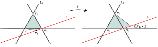
Figure 2: The point ${\tt g}({\tt V}_{2},{\tt V}_{4})$ determines an affine map $T$ between generic quadrilateral configurations.

The other vertices of the triangle $\Delta$ determine rational maps ${\tt g}({\tt V}_{1},\ \ ),\,{\tt g}({\tt V}_{3},\ \ )$, both enjoy analogous properties. ∎

Remark 6.

Three blue lines in Fig. 3 correspond to the fixed points under the reflection symmetries $Sym(3)$ of $\Delta$. By using (26), the complete configuration of six blue lines $N_{1},\ldots,N_{6}$ is invariant under the three transformations ${\tt g}({\tt V}_{j},\ \ )$. We leave this assertion for the reader.

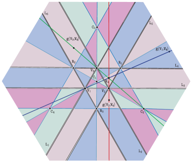
Figure 3: The plane $\mathbb{R}^{2}\backslash\tt A$ with coordinates $\{{\tt x}_{4},{\tt y}_{4}\}$ parametrizes the quadrilateral configurations $\{{\tt V}_{2},{\tt V}_{2},{\tt V}_{3},{\tt V}_{4}=({\tt x}_{4},{\tt y}_{4})\}$. The pair tile $\tt Q={\tt Q}_{1}\cup{\tt Q}_{2}$ is a fundamental domain for the moduli space of quadrilateral configurations, up to $\hbox{\it Aff}\hskip 1.42271pt(\mathbb{K}^{2})$–equivalence. There are 24 copies of the fundamental region ${\tt Q}$. We colored ${\tt Q}_{2}$ and its copies pink or blue (resp. ${\tt Q}_{1}$ and its copies aquamarine or magenta) tiles for strictly convex (resp. non convex) quadrilateral configurations.

Lemma 4.

1. The quotient space of generic quadrilateral configurations up to affine transformations, given by

$$\pi:\mathcal{Q}\longrightarrow\mathcal{Q}/\hbox{\it Aff}\hskip 1.42271pt(\mathbb{K}^{2}),\ \ \ \{(x_{1\,0},y_{1\,0}),\ldots,(x_{4\,0},y_{4\,0})\}\longmapsto[({\tt x}_{4},{\tt y}_{4})],$$ (28)

is a $\mathbb{K}$–analytic surface $\tt Q$.

2. For $\mathbb{K}=\mathbb{C}$, the quotient $\tt Q$ is a connected complex surface.

3. For $\mathbb{K}=\mathbb{R}$, the quotient has two connected components $\tt Q={\tt Q}_{1}\cup{\tt Q}_{2}$ and singular points with local models $\mathbb{K}^{2}/\mathbb{Z}_{2}$ or $\mathbb{K}^{2}/Sym(3)$.

Some comments are in order. Figure 3 illustrates the fundamental domains for $\pi$ over $\mathbb{K}=\mathbb{R}$. The double lines ${\tt A}={\tt L}_{1}\cup\ldots\cup{\tt L}_{6}$ in Fig. 1–4 correspond to forbidden positions for $({\tt x}_{4},{\tt y}_{4})$. Moreover, $({\tt x}_{4},{\tt y}_{4})\in{\tt Q}_{1}$ means a non convex quadrilateral configuration; $({\tt x}_{4},{\tt y}_{4})\in{\tt Q}_{2}$ determines a strictly convex quadrilateral configuration.

Proof.

The set theoretical construction of the quotient is simple, and we describe its projection $\pi$ in (28). Given $\mathcal{P}_{0}\in\mathcal{Q}$, we apply an affine transformation $R\circ T_{j}$ in (24) sending it to

$R\circ T_{j}(\mathcal{P})=\{(0,0),(1,0),(1/2,\sqrt{3}/2),{\tt V}_{4}=({\tt x}_{4},{\tt y}_{4})\}$.

Case 1. The isotropy is trivial $\hbox{\it Aff}\hskip 1.42271pt(\mathbb{K}^{2})_{\mathcal{P}}=id$. There are exactly $24$ different choices for $R\circ T_{j}$, as in Lemma 2; we have that $\pi$ has as target $\mathbb{K}^{2}=\{({\tt x}_{4},{\tt y}_{4})\}$.

In order to describe its analytic properties, recall that the Klein four–group $K$ is isomorphic to $\mathbb{Z}_{2}\times\mathbb{Z}_{2}$. It is such that each element is self–inverse (composing it with itself produces the identity) and composing any two of the three non–identity elements produces the third one; see [2] p. 87. Moreover, the group $Sym(4)$ is of order 24, having a Klein four–group $K$ as a proper normal subgroup; thus $Sym(3)=Sym(4)/K$. We recognize

$$K=\{id,\,{\tt g}({\tt V}_{j},\ \ )\ |\ j\in 1,2,3\}$$

as the group in Lemma 3. Recall (23) and consider the homomorphism given by

$$\varphi:Sym(3)\longrightarrow Aut(K),\ \ \ \sigma\longmapsto\sigma^{-1}_{\alpha}\circ{\tt g}({\tt V}_{j},\ \ )\circ\sigma_{\alpha}({\tt x}_{4},{\tt y}_{4}).$$

The semidirect product of $K$ and $Sym(3)$ determined by $\varphi$ is $Sym(4)=K\rtimes_{\varphi}Sym(3),$ see [2] p. 133. Hence we have a representation of $Sym(4)$ in the birational transformations of $\mathbb{K}^{2}\backslash{\tt A}$ and

$$\tt Q=\frac{\mathcal{Q}}{\hbox{\it Aff}\hskip 1.42271pt(\mathbb{K}^{2})}=\frac{\mathbb{K}^{2}\backslash{\tt A}}{Sym(4)}$$ (29)

is the quotient space. See [16] for a general theory of the quotients of complex manifolds under a discontinuous group of automorphisms. Assertion (1) is done.

For assertion (2), $\mathbb{K}=\mathbb{C}$; note that $\mathbb{K}^{2}\backslash{\tt A}$ is a connected complex manifold. The local behavior of this complex quotient at the points with non trivial isotropy $\mathbb{Z}_{2}$ at the lines ${\tt N}_{1},\,{\tt N}_{2},\,{\tt N}_{3}$ is known to be non–singular (because of C. Chevalley [7], see also [12]). For ${\tt C}$ the isotropy is $Sym(3)$ and the same references describe the local structure of the quotient.

For assertion (3), $\mathbb{K}=\mathbb{R}$; clearly the convexity or non convexity of a quadrilateral configurations are affine invariants, whence there are two connected components. At the points ${\tt C},\ldots,{\tt C}_{4}$ and lines ${\tt N}_{1},\,{\tt N}_{2},\,{\tt N}_{3}$ where the isotropy of the quadrilateral configurations is non trivial, the quotient (29) has singularities; it is an orbifold. ∎

As final step in the proof of Theorem 1, we consider the action on projective classes

$$\mathcal{A}:\hbox{\it Aff}\hskip 1.42271pt(\mathbb{K}^{2})\times Proj(\mathbb{K}[x,y]_{=3})\longrightarrow Proj(\mathbb{K}[x,y]_{=3}),\ \ \ (T,[f])\longmapsto[f\circ T].$$ (30)

This action provides an $\hbox{\it Aff}\hskip 1.42271pt(\mathbb{K}^{2})$–bundle structure on $\mathbb{K}[x,y]_{=3}$. Denote the stabilizer or isotropy group of $[f]\in Proj(\mathbb{K}[x,y]_{=3})$ by

$$\hbox{\it Aff}\hskip 1.42271pt(\mathbb{K}^{2})_{[f]}\doteq\{T\in\hbox{\it Aff}\hskip 1.42271pt(\mathbb{K}^{2})\ |\ f\circ T=\lambda f,\ \lambda\in\mathbb{K}^{*}\}.$$

Equations (15) and (24) provide bijective correspondence between generic quadrilateral configuration in $({\tt x_{4}},{\tt y_{4}})\in\mathbb{K}^{2}\backslash{\tt A}$ and projective classes of polynomials $[f(R^{-1}({\tt x}_{4},{\tt y}_{4}),x,y)]$. If $\mathcal{P}\in{\tt Q}$, then we verify that the isotropy of the quadrilateral configuration $\hbox{\it Aff}\hskip 1.42271pt(\mathbb{K}^{2})_{\mathcal{P}}$ is isomorphic to $\hbox{\it Aff}\hskip 1.42271pt(\mathbb{K}^{2})_{[f]}$. Thus, we have a section

$$f\circ R^{-1}:\mathbb{K}^{2}\backslash\{{\tt A}\}\longrightarrow Proj(\mathbb{K}[x,y]_{=3}),\ \ \ ({\tt x}_{4},{\tt y}_{4})\longmapsto[f(R^{-1}({\tt x}_{4},{\tt y}_{4}),x,y)]$$

and a diagram

(31)

here $\pi$ is the projection of classes from the action (30). The $\hbox{\it Aff}\hskip 1.42271pt(\mathbb{K})$–orbit of a projective class $[f]\in\mathbb{K}[x,y]_{=3}$ is homeomorphic to $\hbox{\it Aff}\hskip 1.42271pt(\mathbb{K}^{2})/\hbox{\it Aff}\hskip 1.42271pt(\mathbb{K}^{2})_{[f]}$. Obviously, $\mathbb{K}[x,y]_{=3,id}$ is open and dense in $\mathbb{K}[x,y]_{=3}$.

The proof of assertion 1, Theorem 1 is done.

Remark 7.

It is well known (see for instance [9] p. 53), that if we consider

$$\mathbb{K}[x,y]_{=3,id}\doteq\{f\in\mathbb{K}[x,y]_{=3}\ |\ \hbox{\it Aff}\hskip 1.42271pt(\mathbb{K}^{2})_{f}={id}\}$$

then the restricted action in $\mathbb{K}[x,y]_{id}$, determines a principal fiber $\hbox{\it Aff}\hskip 1.42271pt(\mathbb{K}^{2})$–bunldle structure. In particular, the quotient $\mathbb{K}[x,y]_{=3,id}/\hbox{\it Aff}\hskip 1.42271pt(\mathbb{K}^{2})$ is a two dimensional $\mathbb{K}$–analytic manifold.

Remark 8.

For $\mathbb{K}=\mathbb{R}$, the fundamental domain ${\tt Q}_{1}\cup{\tt Q}_{2}$ determines the bifurcation diagram of the respective Hamiltonian vector fields, see Fig. 4. By construction, ${\tt Q}_{1}$ has two boundaries and one vertex ${\tt C}$ and ${\tt Q}_{2}$ has one boundary (without extreme points).

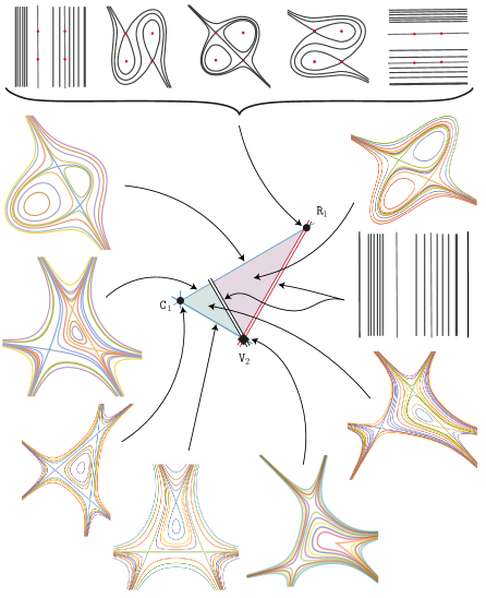
Figure 4: Bifurcation diagram of the real Hamiltonian vector fields $X_{f\circ R^{-1}}$ according to the position of four critical points in the fundamental region $\tt Q$. At the rhombus point $\tt R_{1}$, the configuration of four points $\mathcal{P}=\{(0,0),(1,0),(0,1),{\tt R}_{1}=(1,1)\}\subset\Sigma(f_{\theta})$ is common; see Example 6. The upper row illustrates the topology of $\{f_{\theta}(x,y)\ |\ \theta\in[0,\pi/2]\}$. A saddle connection bifurcation occurs for $\theta=\pi/4$. See %****␣Morse-febrero-2021.tex␣Line␣2275␣****https://github.com/alexander-arredondo/Mathematica-code-for-Essentially-determined-polynomials-of-degree-3/commit/e6a08f9a20da7b23d7a72beff8290af3a23260dc for a code animation in Mathematica of this situation.

We summarize the results in Table 2.

configuration $\mathcal{P}$	cardinality	$dim_{\mathbb{K}}(\mathcal{L}_{3}(\mathcal{P}))$	generators	isotropy
$\{(0,0),(1,0),(0,1),(x_{4},y_{4})\}$	of $\Sigma(f)\vspace{-.3cm}$		of $\mathcal{L}_{3}(\mathcal{P})$	$\hbox{\it Aff}\hskip 1.42271pt(\mathbb{K}^{2})_{\mathcal{P}}$
$(x_{4},y_{4})\in Q$	4	0	eq. (14)	$id$
$(x_{4},y_{4})=(1/3,1/3)=C_{1}$	4	0	$xy(y+x-1)$	$Sym(3)$
$(x_{4},x_{4}),\,x_{4}\neq 0,\,1$	4	0	eq. (14)	$\mathbb{Z}_{2}$
$(x_{4},y_{4})=(1,1)=R_{1}$	4	1	$\begin{array}[]{c}2y^{3}-3y^{2},\ 2x^{3}-3x^{2}\\ \hbox{eq. \eqref{polinomios-rombo}}\end{array}$	$\mathbb{Z}_{2}\times\mathbb{Z}_{4}$
$(1,y_{4})\in L_{5},\ y_{4}\neq\pm 1$	$\infty$	0	$2x^{3}-3x^{2}$	$\hbox{\it Aff}\hskip 1.42271pt(\mathbb{K})$
$\{(0,0),(1,0),(x_{3},0),(x_{4},0)\}$	$\infty$	2	$\begin{array}[]{c}y^{3},xy^{2},y^{2}\\ \hbox{ Lemma \ref{casos-degenerados}.2}\end{array}$	$\mathbb{Z}_{2}$
$\{(0,0),(1,0),(0,1),(0,0)\}$	3, 4 or $\infty$	2	$\begin{array}[]{c}x^{3}-3x^{2},\ y^{3}-3y^{2},\\ x^{2}y+xy^{2}-xy\end{array}$	$\mathbb{Z}_{2}$

Table 2: Dimension, generators and isotropy for $\mathcal{L}_{3}(\mathcal{P})$, where $\mathcal{P}$ is a configuration with 4 points (3 simple points and a double one in the last row).

Example 1.

Relation to the classification of plane cubic curves. The Hesse pencil of cubic curves is

$$\{z^{3}+x^{3}+y^{3}-3\mu zxy=0\},\ \hbox{resp. }\ \{x^{3}+y^{3}-3\mu xy+1=0\},\ \ \ \mu\in\mathbb{C}^{*},$$

in the projective plane $\mathbb{C}\mathbb{P}^{2}=\{[z,x,y]\}$, resp. the affine plane; see [3]. The key property is that any non singular plane cubic is projectively equivalent to a member of the Hesse pencil. The critical points of the affine Hesse polynomial

$f(\mu,x,y)=x^{3}+y^{3}-3\mu xy+1$

determine a generic quadrilateral configuration

$\left\{(0,0),(\mu,\mu),\big{(}-\zeta_{1}\mu,\,\zeta_{2}\mu\big{)},\big{(}\zeta_{2}\mu,\,-\zeta_{1}\mu\big{)}\right\}\subset\mathbb{C}^{2}\backslash\mathbb{R}^{2},$

where $\{1,\zeta_{2},\zeta_{3}\}$ are the cube roots of unity. In order to translate it to our language, up to the linear transformation $M_{\mu}:\mathbb{C}^{2}\longrightarrow\mathbb{C}^{2},\ (x,y)\longmapsto\left(\mu x-\zeta_{2}\mu y,\mu x+\zeta_{3}\mu y\right)$. The quadrilateral configuration changes to

$\mathcal{P}=\{(0,0),(1,0),(0,1),(2\zeta_{1}\mu^{2},\big{(}1+\zeta_{2}\big{)}\mu^{2})\}.$

By Theorem 1, the affine Hesse polynomial

$f(\mu,\ \ ,\ \ )\circ M(x,y)=\mu^{3}\left(2x^{3}-3x(-1+y)y-3x^{2}(1+y)+y^{2}(-3+2y)\right)+1$

is essentially determined. Since these quadrilateral configurations are non real, they are different from the given in Fig. 4.

4.3 Non essential determined polynomials of degree three

By completeness, we describe the polynomials arising from the configurations

$\mathcal{P}=\{(0,0),(1,0),(0,1),(x_{4},y_{4})\}\in{\it Conf}(\mathbb{K}^{2},4)$,  $(x_{4},y_{4})\in\mathscr{A}$.

Lemma 5.

1. Let $\mathcal{P}=\{(0,0),(1,0),(x_{3},0),(x_{4},y_{4})\}$, with $x_{3}\neq 0,1$ and $y_{4}\neq 0$, then $dim_{\mathbb{K}}(Proj(\mathcal{L}_{3}(\mathcal{P})))=0$.

2. Let $\mathcal{P}=\{(0,0),(1,0),(x_{3},0),(x_{4},0)\}$ be a configuration then $dim_{\mathbb{K}}(Proj(\mathcal{L}_{3}(\mathcal{P})))=2$.

Proof.

In assertion (1), up to an affine transformation we can assume $y_{4}=1$. The corresponding cubic polynomial takes the form $f(x,y)=a_{4}\left(2y^{3}-3y^{2}\right)$, where $a_{4}\in\mathbb{K}^{*}$.

For assertion 2, we search for polynomials $f(x,y)\in\mathbb{K}[x,y]^{0}_{\leq 3}$ with at least four affine collinear critical points. The matrix of Eq. (17) results in the cubic polynomials

$f(x,y)=a_{3}xy^{2}+a_{4}y^{3}+a_{7}y^{2}=y^{2}(a_{3}x+a_{4}y+a_{7}),\ \ \ [a_{3},a_{4},a_{7}]\in\mathbb{K}\mathbb{P}^{2},$

with a line of critical points in $\{y=0\}$. ∎

Example 2.

The elementary methods provide an insight in the case of a double point in $\Sigma(f)$. Let $\mathcal{P}_{2}=\{(0,0),(1,0),(0,1),(0,0)\}$ be such a configuration. A basis for $\mathcal{L}_{3}(\mathcal{P}_{2})$ is

$x^{3}-3x^{2},\ y^{3}-3y^{2},\ x^{2}y+xy^{2}-xy.$

The first and second polynomials have lines of singularities, the third one four isolated critical points. The family of polynomials is

$$f(a_{1},a_{2},a_{4},x,y)=a_{1}(x^{3}-3x^{2})+a_{2}(x^{2}y+xy^{2}-xy)+a_{4}(y^{3}-3y^{2}),\ \ \ [a_{1},a_{2},a_{4}]\in\mathbb{K}\mathbb{P}^{2}.$$

As is expected, for values $\left\{(a_{1},a_{2},a_{4}=a_{2}^{2}/9a_{1}\right\}$ the two dimensional family $f(a_{1},a_{2},a_{4},x,y)$ determines polynomials with three isolated singular points, one of them of multiplicity two, see Fig. 4.

5 Degree four polynomials

Let

$$f(x,y)=a_{1}x^{4}+a_{2}x^{3}y+\ldots+a_{13}x+a_{14}y\,\in\mathbb{K}[x,y]^{0}_{\leq 4}$$ (32)

be a polynomial as in (3). Here by notational simplicity we have avoided the double subindex, and let $\mathcal{P}=\{(x_{\iota},y_{\iota})\ |\ \iota\in 1,\ldots,7\}$ be a configuration of seven points. The associated linear system for Eq. (32) is

$$\left(\setcounter{MaxMatrixCols}{14}\begin{smallmatrix}&&&&&\vdots&&&&&&&&\\ 4x_{\iota}^{3}&3x_{\iota}^{2}y_{\iota}^{2}&2x_{\iota}y_{\iota}^{2}&y_{\iota}^{3}&0&3x_{\iota}^{3}&2x_{\iota}y_{\iota}&y_{\iota}^{2}&0&2x_{\iota}&y_{\iota}&0&1&0\\ 0&x_{\iota}^{3}&2x_{\iota}^{2}y_{\iota}&3x_{\iota}y_{\iota}^{2}&4y_{\iota}^{3}&0&x_{\iota}^{2}&2x_{\iota}y_{\iota}&3y_{\iota}^{2}&0&x_{\iota}&2y_{\iota}&0&1\\ &&&&&\vdots&&&&&&&&\end{smallmatrix}\right)\left(\begin{smallmatrix}a_{1}\\ \vdots\\ a_{14}\end{smallmatrix}\right)=\overline{0},\ \ \ \iota=1,\ldots,7.$$ (33)

The interpolation matrix $\phi$, Eq. (33), is square. Hence, for an open and dense set of configurations $\{\mathcal{P}\}\subset{\it Conf}(\mathbb{K}^{2},7)$ such that $\{det(\phi)=0\}$, the resulting space of polynomials of degree four having these $\mathcal{P}$ as critical points is empty. In order to overcome this situation, we introduce the following concept.

Definition 6.

Let $\mathbb{K}[x,y]^{0}_{\leq d}$ with an even dimension and $\delta(d)=\frac{1}{4}\left(d^{2}+3d\right)$ as in (10). Given a configuration $\mathcal{P}_{0}\in{\it Conf}(\mathbb{K}^{2},\delta(d)-1)$, consider a point $(x,y)\in\mathbb{K}^{2}$ and

$$\mathcal{P}_{1}=\Big{\{}\underbrace{(x_{1},y_{1}),\ldots,(x_{\delta(d)-1},y_{\delta(d)-1})}_{\mathcal{P}_{0}},(x,y)\Big{\}}\,\in{\it Conf}(\mathbb{K}^{2},\delta(d)).$$

The interpolation algebraic curve of $\mathcal{P}_{0}$ is

$$\mathcal{I}=\left\{det\big{(}{\phi}(x_{1},y_{1},\ldots,x_{\delta(d)-1},y_{\delta(d)-1},x,y)\big{)}=0\right\}\ \hbox{ in }\mathbb{K}^{2}.$$

Obviously, $\mathcal{I}$ depends on $\mathcal{P}_{0}$, by notational simplicity we omit this dependence. Thus, we have a map

$\mathcal{P}_{0}=\{(x_{1},y_{1}),\ldots,(x_{\delta(d)-1},y_{\delta(d)-1})\}\longmapsto\mathcal{I}.$

Proposition 2.

Let $\mathbb{K}[x,y]^{0}_{\leq d}$ having even dimension.

1. The interpolation curve $\mathcal{I}$ of $\mathcal{P}_{0}$ describes the position of the $\delta(d)$–th point such that $dim_{\mathbb{K}}(\mathcal{L}_{d}(\mathcal{P}_{1}))\geq 0$.

2. There exists a Zariski open set $\{\mathcal{P}_{0}\}\subset{\it Conf}(\mathbb{K}^{2},\delta(d)-1)$ such that the associated $\{\mathcal{I}\}$ are algebraic curves of degree $2d-2$ in $\mathbb{K}^{2}$.

Proof.

For assertion (2), we consider the degree $d$ polynomial

$f(x,y)=a_{1}x^{d}+a_{2}x^{d-1}y+\ldots+a_{\delta(d)-1}x+a_{\delta(d)}y.$

After fixing the configuration $\mathcal{P}_{0}$, the associated linear system only has free variables $x$, $y$, and the linear system is as follows

$$\left(\setcounter{MaxMatrixCols}{14}\begin{smallmatrix}&&&&&\vdots&&&&&&&&\\ (d)x^{d-1}&(d-1)x^{d-2}y&(d-2)x^{d-3}y^{2}&\cdots&0&(d-1)x^{d-2}&\cdots&y^{2}&0&2x&y&0&1&0\\ 0&x^{d-1}&2x^{d-2}y&\cdots&4y^{3}&0&x^{2}&2xy&3y^{2}&0&x&2y&0&1\\ &&&&&\vdots&&&&&&&&\end{smallmatrix}\right)\left(\begin{smallmatrix}a_{1}\\ \vdots\\ a_{\delta(d)}\end{smallmatrix}\right)=\overline{0}.$$ (34)

The determinant of this matrix has $x^{2d-2}$ as higher degree monomial, we are done. ∎

We describe some interpolation curves $\mathcal{I}$.

Example 3.

Let $f\in\mathbb{K}[x,y]^{0}_{\leq 4}$ be a polynomial having degree four and let $\mathcal{P}_{0}=\{(x_{\iota},y_{\iota})\ |\ \iota\in 1,\ldots,6\}$ be a fixed configuration of six different critical points of $f$.

1. If three points of $\mathcal{P}_{0}$ are in a line $\{x=0\}$ and two points are in $\{x=1\}$, then the interpolation curve $\mathcal{I}$, of $\mathcal{P}_{0}$, is given by

$$\mathcal{I}(x,y)=\left(-1152y_{4}^{2}y_{5}^{2}(y_{4}-1)^{2}x_{6}(x_{6}-1)\right)x(x-1)(x-x_{6})g(x,y).$$ (35)

The $\mathcal{I}$ is reducible and singular, it is the product of three parallels lines and a polynomial $g(x,y)$ that pass through the six points in $\mathcal{P}_{0}$.

2. Let $\mathcal{P}_{0}=\{(x_{\iota},y_{\iota})\ |\ \iota\in 1,\ldots,6\}$ be any configuration of six points in the grid of nine points

$\mathcal{G}=\{x(x-1)(x-c_{1})=0\}\cap\{y(y-1)(y-c_{2})=0\}$,   where $c_{1},\,c_{2}\notin\{0,1\}$.

Therefore, the interpolation curve $\mathcal{I}$, associated to the seventh point $(x_{7},y_{7})$, is the product of the six lines defining $\mathcal{G}$.

3. Let $\mathcal{P}=\{(x_{\iota},y_{\iota})\ |\ \iota\in 1,\ldots,6\}$ be a configuration of six critical points of $f$. If the six points are distributed in a conic $Q$, then the interpolation curve $\mathcal{I}$, associated to the seventh point $(x_{7},y_{7})$, contains the conic. That is, $\mathcal{I}=Qg$ for some $g\in\mathbb{K}[x,y]^{0}_{\leq 4}$.

A complete study of the interpolation curves $\mathcal{I}$ arising from configurations of six points is the goal of a future project.

6 Pencils of polynomial vector fields

Now we will consider some special configurations of $(d-1)^{2}\geq 4$ points.

Definition 7.

Let $\{F(x,y)=0\},\ \{G(x,y)=0\}$ be two algebraic curves in $\mathbb{K}^{2}$, both of degree $d-1$ $(\geq 2)$. We assume that they have transversal intersection in exactly $(d-1)^{2}$ affine points, thus

$$\mathcal{P}_{ci}=\{F(x,y)=0\}\cap\{G(x,y)=0\}\in{\it Conf}(\mathbb{K}^{2},(d-1)^{2})$$ (36)

is a complete intersection configuration. The associated pencil of curves is

$$\left\{\mu F(x,y)+\nu G(x,y)=0\ |\ [\mu,\nu]\in\mathbb{K}\mathbb{P}^{1}\right\}.$$ (37)

$\mathcal{P}_{ci}$ is the base locus of the pencil of curves.

Moreover, the choice of an ordered pair of polynomial functions from (37), not just curves say

$\big{(}{\tt a}F(x,y)+{\tt b}G(x,y),\ {\tt c}F(x,y)+{\tt d}G(x,y)\big{)}$

determines a $SL(2,\mathbb{K})$–pencil of polynomial vector fields

$$\mathfrak{F}(\mathcal{P}_{ci})=\left\{\ X_{\tt M}=-\big{(}{\tt c}F(x,y)+{\tt d}G(x,y)\big{)}\frac{\partial}{\partial x}+\big{(}{\tt a}F(x,y)+{\tt b}G(x,y)\big{)}\frac{\partial}{\partial y}\ \Big{|}\ {\tt M}=\left(\begin{smallmatrix}\tt{-c}&\tt{-d}\\ \ \tt{a}&\ \tt{b}\end{smallmatrix}\right)\in SL(2,\mathbb{K})\ \right\}.$$ (38)

The condition $det({\tt M})\neq 0$ is equivalent with the fact the zero locus of the vector field $X_{\tt M}$ coincides with $\mathcal{P}_{ci}$.

Lemma 6.

Let $\mathcal{U}_{d}\subseteq\mathfrak{X}(\mathbb{K}^{2})_{\leq d-1}$ be the open and dense set of polynomial vector fields of degree $d-1$, having exactly $(d-1)^{2}$ zeros in $\mathcal{P}_{ci}\subset{\it Conf}(\mathbb{K}^{2},(d-1)^{2})$. Assume that $\mathcal{P}_{ci}$ has trivial isotropy group in $\hbox{\it Aff}\hskip 1.42271pt(\mathbb{K}^{2})$. In $\mathcal{U}_{d}$ there exists an analytic $SL(2,\mathbb{K})$–bundle structure as follows

(39)

Proof.

We want to show that a polynomial vector field $X\in\mathfrak{X}(\mathbb{K}^{2})_{\leq d-1}$ has $(d-1)^{2}$ zeros exactly at $\mathcal{P}_{ci}$ as in (36) if and only if it is of the shape $X_{\tt M}$ in (38).

($\Rightarrow$) Let $X=A(x,y)\frac{\partial}{\partial x}+B(x,y)\frac{\partial}{\partial y}$ be a vector field in $\mathfrak{X}(\mathbb{K}^{2})_{\leq d-1}$. The curve $\mathcal{C}_{A}\doteq\{A(x,y)=0\}$ has at most degree $d-1$ and it would contain $\mathcal{P}_{ci}$. There exist an open set of values $\{[\mu,\nu]\}\subset\mathbb{K}\mathbb{P}^{1}$ such that for each value the respective curve $\{\mu F+\nu G=0\}$ in the pencil (37) intersects in a transversal way $\mathcal{C}_{A}$ at every point of $\mathcal{P}_{ci}$. By Bézout’s theorem, the degree of $\mathcal{C}$ is exactly $d-1$. For any point $p\in\mathcal{C}_{A}\backslash\mathcal{P}_{ci}\subset\mathbb{K}^{2}$, there exists a value, say $[-{\tt c},-{\tt d}]$ in (37) such that its respective curve satisfies $\mathcal{C}_{-{\tt c}-{\tt d}}\cap\mathcal{C}_{A}\supset\widehat{\mathcal{P}}\cup\{p\}$. Hence (again by Bézout’s theorem), both curves coincide as sets and $A=-{\tt c}F-{\tt d}G$ as polynomials. ∎

Thus, each configuration $\mathcal{P}_{ci}$ has an associated fiber $\big{\{}X_{\tt M}\ |\ {\tt M}\in SL(2,\mathbb{K})\big{\}}\subset\mathcal{U}_{d}$ in (39), which is a family of not necessarily Hamiltonian vector fields. A further goal is the study of the intersection

$$\big{\{}X_{\tt M}\ |\ {\tt M}\in SL(2,\mathbb{K})\big{\}}\cap Ham(\mathbb{K}^{2})_{\leq d}.$$

Corollary 3.

A jump phenomena. Let $\mathcal{P}=\{(0,0),(1,0),(1/2,\sqrt{3}/2),(x_{4},y_{4})\}$ be a configuration leading to a family of vector fields $\mathfrak{F}(\mathcal{P})=\{X_{\tt m}\ |\ {\tt m}\in SL(2,\mathbb{K})\}$ as in (38).

1. If $(x_{4},y_{4})\in\mathbb{K}^{2}\backslash{\tt A}$, then there exists one projective class in $\mathfrak{F}(\mathcal{P})\cap Ham(\mathbb{K}^{2})\leq_{2}$.

2. If $(x_{4},y_{4})={\tt R}_{1},\,{\tt R}_{2}$ or ${\tt R}_{3}$, then there exists a $\mathbb{KP}^{1}$–family of Hamiltonian vector fields $\mathfrak{F}(\mathcal{P})\cap Ham(\mathbb{K}^{2})_{\leq_{2}}$. $\Box$

Example 4.

A family $\big{\{}X_{\tt M}\ |\ {\tt M}\in SL(2,\mathbb{K})\big{\}}$ in (39) with $(d-1)^{2}\geq 4$ points as base locus and such that its Hamiltonian vector fields $Ham(\mathbb{K}^{2})_{\leq d-1}=[f]$ determine one projective class.

Consider two algebraic curves such that

$$\mathcal{P}_{ci}=\{\underbrace{y-\mu\Pi_{\iota=1}^{d}(x-x_{\iota})=0}_{F(x,y)=0}\}\cap\{\underbrace{x-\nu\Pi_{j=1}^{d}(y-y_{j})=0}_{G(x,y)=0}\},\ \ \ d\geq 3$$

has exactly $(d-1)^{2}\geq 4$ points.

It follows that, the associated 1–form $\omega_{\tt m}$ is exact if and only if ${\tt m}=\left(\begin{smallmatrix}\tt{a}&\tt{0}\\ \ \tt{0}&\tt{a}\end{smallmatrix}\right)$. In fact, suppose $f(x,y)$ such that $\omega_{\tt m}=df$, then

${\tt a}F(x,y)+{\tt b}G(x,y)=f_{x}$  and  ${\tt c}F(x,y)+{\tt d}G(x,y)=f_{y}$.

As $f_{xy}=f_{yx}$, then ${\tt a}-{\tt b}\frac{\partial}{\partial y}\Pi_{j=1}^{d}(y-y_{j})=-{\tt c}\frac{\partial}{\partial x}\Pi_{\iota=1}^{d}(x-x_{\iota})+{\tt d}$, so ${\tt a}={\tt d}$ and ${\tt b}={\tt c}=0$.

By assumption $\omega_{\tt m}$ is exact and defining $f_{\tt m}(x,y)=\int^{(x,y)}\omega_{\tt m}$, we conclude that

$$\mathfrak{F}(\mathcal{P}_{ci})\cap Ham(\mathbb{K}^{2})_{\leq d-1}=\mathcal{L}_{d}(\mathcal{P}_{ci})=[f_{\tt m}]\ \ \ \hbox{ and }\ \ \ dim_{\mathbb{K}}(\mathcal{L}_{d}(\mathcal{P}_{ci}))=0.$$ (40)

Example 5.

A fiber $\big{\{}X_{\tt M}\ |\ {\tt M}\in SL(2,\mathbb{K})\big{\}}$ as in (39) with $(d-1)^{2}\geq 9$ points as a base locus and such that

$\big{\{}X_{\tt M}\ |\ {\tt M}\in SL(2,\mathbb{K})\big{\}}\cap Ham(\mathbb{K}^{2})_{=d}=\emptyset$.

Consider two hyperelliptic curves such that

$$\widehat{\mathcal{P}}=\{F(x,y)=y^{2}-\mu\Pi_{\iota=1}^{d}(x-x_{\iota})=0\}\cap\{G(x,y)=x^{2}-\nu\Pi_{j=1}^{d}(y-y_{j})=0\}$$

has exactly $(d-1)^{2}\geq 9$ points. It follows that $\omega_{\tt m}$ is non exact for all ${\tt m}=\left(\begin{smallmatrix}\tt{a}&\tt{b}\\ \tt{c}&\tt{d}\end{smallmatrix}\right).$ We conclude that

$$\mathcal{L}_{d}(\widehat{\mathcal{P}})=\emptyset\ \ \ \hbox{ and }\ \ \ dim_{\mathbb{K}}(\mathcal{L}_{d}(\widehat{\mathcal{P}}))=-1.$$ (41)

In fact, if we suppose $f(x,y)$ such that $\omega_{m}=df$, then $2{\tt a}y-{\tt b}\frac{\partial}{\partial y}\Pi_{j=1}^{d}(y-y_{j})=-{\tt c}\frac{\partial}{\partial x}\Pi_{\iota=1}^{d}(x-x_{\iota})+2{\tt d}x$, so ${\tt a}={\tt b}={\tt c}={\tt d}=0$.

Corollary 4.

There exists a fiber $\mathfrak{F}$ as in (39) having $d^{2}$ points as base locus and

$\mathfrak{F}(\widehat{\mathcal{P}})\cap Ham(\mathbb{K}^{2})_{=d}=\mathbb{K}\mathbb{P}^{1}.$

Moreover, $\mathbb{K}\mathbb{P}^{1}$ minus a finite set determines Morse polynomials.

The above result uses the following very particular configurations.

Definition 8.

A grid of $(d-1)^{2}$ points $\mathcal{G}$ is determined by two sets of $d-1$ parallel lines where one set is transverse to the other, i.e. up to affine transformation

$$\mathcal{G}=\{F(x,y)=\Pi_{j=1}^{d-1}(y-y_{j})=0\}\cap\{G(x,y)=\Pi_{\iota=1}^{d-1}(x-x_{\iota})=0\}$$

with exactly $(d-1)^{2}\geq 4$ points (it is a complete intersection).

Proof of the Corollary. The family $X_{\tt M}$ with a grid of $(d-1)^{2}$ points is Hamiltonian if and only if

${\tt M}\in\left\{\left(\begin{smallmatrix}0&-{\tt d}&\\ {\tt a}&0\end{smallmatrix}\right)\right\}\cong\mathbb{K}^{2}\subset SL(2,\mathbb{K})$.

In fact, $\omega_{\tt m}=({\tt a}F(x)+{\tt b}G(y))dx+({\tt c}F(x)+{\tt d}G(y))dy=0$ is exact if and only if ${\tt b}G(y)_{y}={\tt c}F(x)_{x}$. The equality holds only for ${\tt b}={\tt c}=0$.

The respective vector subspace of polynomials

$$\left\{f({\tt a},{\tt d},x,y)={\tt a}\int^{(x,y)}\Pi_{\iota=1}^{d}(x-x_{\iota})dx+{\tt d}\int^{(x,y)}\Pi_{j=1}^{d}(y-y_{j})dy\ \Big{|}\ ({\tt a},{\tt d})\in\mathbb{K}^{2}\backslash\{\overline{0}\}\ \right\}\subset\mathbb{K}[x,y]^{0}_{\leq d}$$ (42)

shows that

$$\mathcal{L}_{d}(\mathcal{P})\supset\{[f({\tt a},{\tt d},x,y)]\}\ \ \ \hbox{ and }\ \ \ dim_{\mathbb{K}}(\mathcal{L}_{d}(\mathcal{P}))=1.$$ (43)

For $({\tt a},{\tt d})\neq({\tt a},0),\,(0,{\tt d})$, each polynomial $f({\tt a},{\tt d},x,y)\in\mathbb{K}[x,y]^{0}_{\leq d}$ in (42) has $(d-1)^{2}$ Morse critical points. In fact, at each point $p\in\mathcal{P}$ a very simple observation with the Taylor series shows that $f({\tt a},{\tt d},x,y)=\widetilde{\tt a}x^{2}+\widetilde{\tt b}y^{2}+\mathcal{O}_{3}(x,y)$, where $\widetilde{\tt a}\widetilde{\tt b}\neq 0$.

On the other hand, for $({\tt a},{\tt d})=({\tt a},0),\,(0,{\tt d})$ the polynomial $f({\tt a},{\tt d},x,y)$ has lines of critical points in $\{P(x,y)=0\}$ or $\{Q(x,y)=0\}$. $\Box$

Example 6.

Real rotated Hamiltonian vector fields for the grid of $4$ points. Let $\mathcal{G}=\{(0,0),(1,0),(0,1),R=(1,1)\}$ be a grid its space of polynomials is

$f({\tt a},{\tt d},x,y)={\tt a}\Big{(}\dfrac{x^{3}}{3}-\dfrac{x^{2}}{2}\Big{)}+{\tt d}\Big{(}\frac{y^{3}}{3}-\frac{y^{2}}{2}\Big{)}.$

In particular for $\mathbb{K}=\mathbb{R}$, we consider the family

$R_{\theta}=\left\{f_{\theta}(x,y)=\cos(\theta)\big{(}\frac{x^{3}}{3}-\frac{x^{2}}{2}\big{)}+\sin(\theta)\big{(}\frac{y^{3}}{3}-\frac{y^{2}}{2}\big{)}\ \Big{|}\ \theta\in[0,2\pi]\right\}$

of polynomials in (42). They originate a family of rotated vector fields, see Fig. 4. The algebraic curve $\{f_{\theta}(x,y)+c=0\}$ is reducible for $\theta=\pi/4$ and $c={1/6}$. In this case we get

$\{(x+y-1)(2y^{2}-2xy+2x^{2}-y-x-1)=0\}$.

The following family of vector fields is related to the results in [17] §5; see Fig. 4, upper row.

Corollary 5.

The one dimensional holomorphic family of Hamiltonian vector fields of the polynomials

$\left\{f({\tt a},{\tt d},x,y)={\tt a}\Big{(}\dfrac{x^{3}}{3}-\dfrac{x^{2}}{2}\Big{)}+{\tt d}\Big{(}\frac{y^{3}}{3}-\frac{y^{2}}{2}\Big{)}\ \big{|}\ {\tt ad}=1\right\}$

has singularities at $\mathcal{G}=\{(0,0),(1,0),(0,1),R=(1,1)\}$ and spectra of eigenvalues

$\big{[}[i,\,-i],\,[1,-1],\,[i,\,-i],\,[1,-1]\big{]}$.

$\Box$

Corollary 6.

For $d\geq 3$, there exist Morse polynomials $f\in\mathbb{K}[x,y]_{=d}^{0}$ with $(d-1)^{2}$ singular points that are not essentially determined. $\Box$

7 Closing remarks

Let $\mathfrak{X}(\mathbb{K}^{2})_{\leq d-1}$ be the space of polynomial vector fields $\{X\}$ of at most degree $d-1$ on $\mathbb{K}^{2}$. A general and natural question is as follows. Under what conditions a polynomial vector field $X$ on $\mathbb{K}^{2}$ is essentially determined by its configuration of zeros $\mathcal{Z}(X)$ in $\mathbb{K}^{2}$?

In simple words, a vector field $X$ is essentially determined (in $\mathfrak{X}(\mathbb{K}^{2})_{\leq d-1}$) by its configuration of zeros $\mathcal{Z}(X_{f})$,

if for any $Y\in\mathfrak{X}(\mathbb{K}^{2})_{\leq d-1}$ satisfying $\mathcal{Z}(X)\subset\mathcal{Z}(Y)\subset\mathbb{K}^{2}$, then $X=\lambda Y$.

Recalling that for affine degree $d$ the number of isolated singularities of the associated singular holomorphic foliation $\mathcal{F}(\mathcal{X})$ on the whole $\mathbb{CP}^{2}$ is $(d-1)^{2}+d$, the hypothesis of multiplicity one must be understood for all these points. Proposition 1 confirms that in the Hamiltonian case only $\delta(d)\leq(d-1)^{2}$ points are required.

Recall that X. Gómez–Mont and G. Kempf, [13], established in the complex rational case the following deep result, that also enlightens the real case.

A meromorphic vector field $\mathcal{X}$ on $\mathbb{CP}^{m}$, $m\geq 2$, of degree $r\geq 2$, with critical points having all its zeros of multiplicity one is completely determined by its zero set.

Moreover, J. Artes, J. Llibre, D. Schlomiuk and N. Vulpe, [4], [5] prove the following:

A polynomial vector field $\mathcal{X}$ on $\mathbb{K}^{2}$ of degree two, is completely determined by the position of its seven critical points (including the points at infinity).

As far as we know, over $\mathbb{K}=\mathbb{C}$ the more general result is due to A. Campillo and J. Olivares, [6]:

A singular holomorphic foliation $\mathcal{X}$ on $\mathbb{CP}^{2}$ of degree $r\geq 2$, w is completely determined by its singular scheme.

See C. Alcántara et al. [1] for recent developments regarding foliations with multiple points. We summarize our results as follows.

Corollary 7.

A polynomial Hamiltonian vector field $X_{f}$ on $\mathbb{K}^{2}$ of degree two is completely determined (in the space of polynomial vector fields of degree $2$, up to a scalar factor $\lambda\in\mathbb{K}^{*}$) by its zero points, when they are four isolated points different from $\{(0,0),\,(1,0),\,(0,1),\,(1,1)\}$, up to affine transformation.

Our hope is that the explicit results in this paper can illustrate the classification of polynomials $\mathbb{K}[x,y]$ up to algebraic equivalence $Aut(\mathbb{K}^{2})$; see [11] and [18] for this order of ideas. This potential application is the subject of a future project.

References

- [1] C. R. Alcántara, R. Pantaleón–Mondragón, Foliations on with a unique singular point without invariant algebraic curves, Geom. Dedicata, 207 (2020), 193–200. https://doi.org/10.1007/s10711-019-00492-8
- [2] M. A. Amstrong, Groups and Symmetry, Springer–Verlag, New York, 1988. https://doi.org/10.1007/978-1-4757-4034-9
- [3] M. Artebani, I. Dolgachev, The Hesse pencil of plane cubic curves, Enseign. Math., (2), 25, 55 (2009), 235–273. https://doi.org/10.4171/LEM/55-3-3
- [4] J. C. Artés, J. Llibre, N. Vulpe, When singular points determine quadratic systems, Electron. J. Differential Equations, Vol. 2008, 82 (2008), 1–37. https://ejde.math.txstate.edu/Volumes/2008/82/artes.pdf
- [5] J. C. Artes, J. Llibre, D. Schlomiuk, N. Vulpe, From topological to geometric equivalence in the classification of singularities at infinity for quadratic vector fields, Rocky Mountain J. Math., 45, 1 (2015), 29–113. https://core.ac.uk/download/pdf/78533785.pdf
- [6] A. Campillo, J. Olivares, Polarity with respect to a foliation and Cayley–Bacharach theorem, J. reine angew. Math., 534 (2001), 95–118. https://doi.org/10.1515/crll.2001.036
- [7] C. Chevalley, Invariants of finite groups generated by reflections, Amer. J. Math., 77 (1955), 778–782. https://doi.org/10.2307/2372597
- [8] C. Ciliberto, Geometric aspects of polynomial interpolation in more variables and of Waring’s problem, European Congress of Mathematics, Vol. I, (Barcelona, 2000), 289–316, Progr. Math, 201, Birkhaüser, Basel, 2001. https://www.math.uni-bielefeld.de/~rehmann/ECM/cdrom/3ecm/pdfs/pant3/cilibet.pdf
- [9] J. J. Duistermaat, J. A. C. Kolk, Lie Groups, Springer–Verlag, Berlin, 1999. https://doi.org/10.1007/978-3-642-56936-4
- [10] D. Eisenbud, J. Harris, The Geometry of Schemes, GTM 197, Springer–Verlag, New York, 2000. https://doi.org/10.1007/b97680
- [11] J. Fernández de Bobadilla, Moduli of Polynomials in Two Variables, Memoirs AMS, Providence, 2005. https://doi.org/10.1090/memo/0817
- [12] L. Flatto, Invariants of finite reflection groups, Enseign. Math., (2), 24, 3–4, (1978), 237–292. https://www.e-periodica.ch/cntmng?pid=ens-001%3A1978%3A24%3A%3A111
- [13] X. Gómez–Mont, G. Kempf, Stability of meromorphic vector fields in projective spaces, Comm. Math. Helv., 64 (1989), 462–473. https://doi.org/10.1007/BF02564687
- [14] T. de Jong, G. Pfister, Local Analytic Geometry, Vieweg, Braunschweig/Wiesbaden, 2000. https://doi.org/10.1007/978-3-322-90159-0
- [15] R. Miranda, Linear systems of plane curves, Notices AMS, 46, 2 (1999), 192–202. https://www.ams.org/journals/notices/199902/miranda.pdf
- [16] D. Prill, Local classification of quotients of complex manifolds by discontinuous groups, Duke Math. J., 34 (1967), 375–386. https://doi.org/10.1215/S0012-7094-67-03441-2
- [17] V. Ramírez, Twin vector fields and independence of spectra for quadratic vector fields, J. Dyn. Control Syst., 23 (2017), 623–633. https://link.springer.com/article/10.1007/s10883-016-9344-5
- [18] P. G. Wightwick, Equivalence of polynomials under automorphisms of , J. Pure Appl. Algebra, 157 (2001), 341–367. https://doi.org/10.1016/S0022-4049(00)00014-1