Convergence and Recovery Guarantees of the K-Subspaces Method
for Subspace Clustering

Abstract

The K-subspaces (KSS) method is a generalization of the K-means method for subspace clustering. In this work, we present local convergence analysis and a recovery guarantee for KSS, assuming data are generated by the semi-random union of subspaces model, where $N$ points are randomly sampled from $K\geq 2$ overlapping subspaces. We show that if the initial assignment of the KSS method lies within a neighborhood of a true clustering, it converges at a superlinear rate and finds the correct clustering within $\Theta(\log\log N)$ iterations with high probability. Moreover, we propose a thresholding inner-product based spectral method for initialization and prove that it produces a point in this neighborhood. We also present numerical results of the studied method to support our theoretical developments.

1 Introduction

Subspace clustering (SC) is a fundamental problem in unsupervised learning, which can be applied to do dimensionality reduction and data analysis. It has found wide applications in diverse fields, such as computer vision (Ho et al., 2003; Vidal et al., 2008), gene expression analysis (Jiang et al., 2004; Ucar et al., 2011), and image segmentation (Hong et al., 2006), to name a few. In research on SC, the union of subspace (UoS) model, which assumes that data points lie in one of multiple underlying subspaces, is a typical model for studying SC. In particular, substantial advances have been made recently on designing algorithms for solving the SC problem and on establishing theoretical foundations in the UoS model; see, e.g., Vidal (2011); Vidal et al. (2016); Meng et al. (2018) and the references therein.

In the UoS model, the goal of SC is to recover the underlying subspaces and cluster the unlabeled data points into the corresponding subspaces. To achieve this goal, many algorithms have been proposed in the past two decades, such as sparse subspace clustering methods (Elhamifar & Vidal, 2013; Wang & Xu, 2013), low-rank representation-based methods (Liu et al., 2012), thresholding-based methods (Heckel & Bölcskei, 2015; Li & Gu, 2021), and K-subspaces (KSS) method (Bradley & Mangasarian, 2000). In these methods, the KSS method, which is known as a generalization of the K-means method, can handle clusters in subspaces. In particular, it is conceptually simple and has linear complexity per iteration. This computational benefits render it suitable to handle large-scale datasets in practice. However, a complete theoretical understanding of its convergence behavior and recovery performance is not found in the literature, to the best of our knowledge. This is due in part to its alternating and discrete nature, as well as the fact that as with the K-means, KSS can easily get stuck in bad local minima without a good initialization. Consequently, it remains a major challenge to provide the theoretical foundations for KSS. In this work, we provide guarantees for the convergence behavior and recovery performance of the KSS method. We also develop a simple initialization method with provable guarantees for the KSS method. It is worth mentioning that our results improve on state-of-the-art theory with respect to allowable affinity between subspaces, and support the algorithm’s competitive performance in our numerical evaluation.

1.1 Related Works

Over the past years, a substantial body of literature explores algorithmic development and theoretical analysis of SC. One of the most well-studied methods is arguably sparse subspace clustering (SSC), which is motivated by representing each data point as a sparse linear combination of the remaining ones. A seminal work by Elhamifar & Vidal (2013) proposed and studied this method. The algorithm proceeds by solving a convex sparse optimization problem, followed by applying spectral clustering to the graph constructed by a solution of this convex problem. In particular, they showed that when the data points are drawn from the disjoint subspaces in the noiseless setting, the solution is non-trivial and no edges in the constructed graph connect two points in different subspaces. This is referred to as the subspace detection property (SDP) in literature; see, e.g., Wang & Xu (2013); Soltanolkotabi et al. (2012, 2014). We should point out that SDP does not imply correct clustering (CC) of data points as mentioned in Wang et al. (2016); Li & Gu (2021). Following this line of work, theoretical results on the SSC method in various contexts have been established, and many variants and extensions of the SSC method have been proposed. For example, Soltanolkotabi et al. (2012) developed a unified analysis framework of the SSC method, which showed that the SDP holds even when subspaces can be overlapping in the noiseless setting. Later, Soltanolkotabi et al. (2014) extended their analysis and results to the noisy setting. Meanwhile, an independent work by Wang & Xu (2013) also studied the behavior of SSC based on the SDP in the noisy setting. In spite of the solid theoretical guarantees and great empirical performance, SSC suffers from high computational cost. To tackle this issue, Dyer et al. (2013) applied an orthogonal matching pursuit (OMP) method to SSC. Then, Tschannen & Bölcskei (2018) analyzed the performance of this method in the noisy setting and also introduced and studied the matching pursuit (MP) method for SSC. Recently, more and more variants and extensions for solving SSC have been proposed; see, e.g., Ding et al. (2021); Wang et al. (2019); Wu et al. (2020); Chen et al. (2020); Matsushima & Brbic (2019); Traganitis & Giannakis (2017); You et al. (2016).

Table 1: Comparison of affinity requirement and recovery results of the surveyed methods in the noiseless semi-random UoS model with overlapping subspaces ($K\geq 2$).

References	Methods	Affinitya	Results
Soltanolkotabi et al. (2012)	SSC	$O(\frac{1}{\sqrt{\log N}})$	SDP
Wang & Xu (2013)	SSC	$O(\frac{1}{\sqrt{\log N}})$	SDP
Tschannen & Bölcskei (2018)	(O)MP	$O(\frac{1}{\sqrt{\log N}})$	SDP
Wang et al. (2016)	SSC	$O(\frac{1}{\sqrt{\log N}})$	CC
Heckel & Bölcskei (2015)	TSC	$O(\frac{1}{\sqrt{\log N}})$	CC
Park et al. (2014)	GSR	$O(\frac{1}{\sqrt{\log N}})^{b}$	CC
Lipor et al. (2021)	EKSS	$O(\frac{1}{\sqrt{\log N}})$	CC
Ours	KSS	$O(1)$	CC

^aWe use the notion (15) to measure the subspace affinity. ^bThis is obtained by taking $\delta=1/N$ in Park et al. (2014, Theorem 3.2).

As for other methods for SC, Liu et al. (2012) proposed a low-rank representation (LRR) method by minimizing a nuclear norm regularized problem. In particular, they showed that the proposed method can recover the row space of the data points. Later, Shen et al. (2016) developed an online version of the LLR method, which reduces its computational cost significantly. Another notable approach for SC is thresholding-based methods, which exploit the correlation between data points. For example, Heckel & Bölcskei (2015) proposed a thresholding-based subspace clustering (TSC) method, which applies spectral clustering to a weight matrix with entries depending on spherical distances of each data point to its nearest neighbors. They showed that TSC can achieve correct clustering by proving that the formed graph has no false connection and $K$ connected subgraphs. Li & Gu (2021) proposed a thresholding inner-product (TIP) method for SC, which constructs an adjacency matrix by thresholding magnitudes of inner products between data points. In particular, they provided an explicit bound on the error rate of the TIP method when there are only two subspaces of the same dimension. Moreover, Park et al. (2014) proposed a greedy subspace clustering (GSC) method that constructs a neighborhood matrix using a nearest subspace neighbor method and then recovers subspaces by a greedy algorithm. They showed that their approach can guarantee correct clustering. However, they assumed that the dimension of each subspace is known and same and the number of data points in each subspace is also same. Actually, there are still numerous other popular methods using different techniques for SC, such as matrix factorization-based method (Boult & Brown, 1991; Pimentel-Alarcón et al., 2016; Fan, 2021) and principal component analysis type methods (Vidal et al., 2005; McWilliams & Montana, 2014).

In contrast to the above methods, the KSS method (Bradley & Mangasarian, 2000; Agarwal & Mustafa, 2004; Tseng, 2000) is essentially a generalization of the k-means method for SC, which minimizes the sum of distances of each point to its projection onto the assigned subspace, i.e.,

$$\min_{\mathcal{C},\bm{U}}\ \sum_{k=1}^{K}\sum_{i\in\mathcal{C}_{k}}\|\bm{z}_{i}-\bm{U}_{k}\bm{U}_{k}^{T}\bm{z}_{i}\|^{2},$$ (1)

where $\{\bm{z}_{i}\}_{i=1}^{N}\subseteq\mathbb{R}^{n}$ denotes the set of $N$ data points, $\mathcal{C}=\{\mathcal{C}_{k}\}_{k=1}^{K}$ denotes the set of $K\geq 2$ estimated clusters, and $\bm{U}=\begin{bmatrix}\bm{U}_{1}&\dots&\bm{U}_{K}\end{bmatrix}$ with $\bm{U}_{k}$ being an orthonormal basis of the corresponding cluster. Similar to the k-means method, the KSS method proceeds by alternating between the subspace update step and the cluster assignment step. As a local search algorithm, it is conceptually simple and has linear complexity as a function of the number of data points, while many popular methods based on self-expression property, such as the surveyed SSC, OMP-based SSC, and LLR, have at least quadratic complexity. This computational advantage renders it more suitable to handle large-scale datasets than these self-expression property based-methods. However, due to its non-convex nature, it suffers from sensitivity to initialization and lack of theoretical understanding. To fix the former issue, some heuristics for good initialization have been proposed; see, e.g., He et al. (2016); Zhang et al. (2009). To improve the performance of the KSS method, Gitlin et al. (2018) employed a coherence pursuit algorithm. Recently, Lipor et al. (2021) applied an ensembles approach to the KSS method with random initialization and showed that it achieves correct clustering based on the argument in Heckel & Bölcskei (2015). However, their analysis can only tackle one KSS iteration. Generally, it remains open to propose a provable initialization scheme for the KSS method and fully understand its convergence behavior and recovery performance. Due to this, the KSS method has mostly been superseded by convex methods based on self-expression property, which are widely studied and have solid theoretical results. Moreover, establishing theoretical foundations for the KSS method may open the door for the study of various non-convex methods for SC.

1.2 Our Contributions

In this work, we study the KSS method for SC in the semi-random UoS model. First, we provide theoretical guarantees for the convergence behavior and recovery performance of the KSS method. Specifically, we prove the existence of a basin of attraction, whose radius is as large as $O(\sqrt{N})$ around the true clustering of the data points, when the cluster sample sizes are on the same order and the subspace dimensions are also on the same order. If the initial assignment of the KSS method lies within this basin, the algorithm is guaranteed to converge to the true clustering at a superlinear rate. In particular, once the number of iterations reaches $\Theta(\log\log N)$, the KSS method yields the true clustering with the corresponding orthonormal bases exactly. It is worth emphasizing that these results are obtained under the condition that the normalized affinity between pairwise subspaces is $O(1)$, which is generally milder than those in the existing literature; see the comparison in Table 1. Second, we propose a thresholding inner-product based spectral method for initialization of the KSS method. We show that it can generate a point lying in the basin of attraction of the KSS method by deriving its clustering error rate. Our core argument is to derive a spectral bound for a random adjacency matrix without independence structure, which could be of independent interest. In conclusion, our work demystifies the computational efficiency of the KSS method and provides a provable initialization scheme for it, thus bridging the gap between theory and practice. From a broader perspective, our work also contributes to the literature on simple and scalable non-convex methods with provable guarantees; see, e.g., Wang et al. (2021a, b); Zhang et al. (2020); Gao & Zhang (2019); Boumal (2016); Ling (2022).

Notation. Let $\mathbb{R}^{n}$ be the $n$-dimensional Euclidean space and $\|\cdot\|$ be the Euclidean norm. Given a matrix $\bm{A}$, we use $\|\bm{A}\|$ to denote its spectral norm, $\sigma_{i}(\bm{A})$ its $i$-th largest singular value, $\|\bm{A}\|_{F}$ its Frobenius norm, and $a_{ij}$ its $(i,j)$-th element. Given a vector $\bm{a}\in\mathbb{R}^{n}$, we denote by $a_{i}$ its $i$-th element. Given a positive integer $n$, we denote by $[n]$ the set $\{1,\dots,n\}$. Given $d_{1},\dots,d_{K}$, let $d_{\min}=\min\{d_{k}:k\in[K]\}$ and $d_{\max}=\max\{d_{k}:k\in[K]\}$. Given a discrete set $S$, we denote by $|S|$ its cardinality. Given two sets $A,B\subseteq[n]$, the set difference between $A$ and $B$ denoted by $A\setminus B$ is defined by $A\setminus B=\{x\in A:x\notin B\}$. We use $\mathcal{O}^{n\times d}$ to denote the set of all $n\times d$ matrices that have orthonormal columns (in particular, $\mathcal{O}^{d}$ denotes the set of all $d\times d$ orthogonal matrices) and $\Pi_{K}$ to denote the set of all $K\times K$ permutation matrices. Let $\pi:[K]\rightarrow[K]$ denote a permutation of the elements in $[K]$. Each $\pi$ corresponds to a $\bm{Q}_{\pi}=\{q_{ij}\}_{1\leq i,j\leq K}\in\Pi_{K}$ such that $q_{ij}=1$ if $j=\pi(i)$ and $q_{ij}=0$ otherwise for all $i\in[K]$. The converse also holds. Moreover, for any $\bm{U},\bm{V}\in\mathcal{O}^{n\times d}$, we denote by $d(\bm{U},\bm{V})=\left\|\bm{U}\bm{U}^{T}-\bm{V}\bm{V}^{T}\right\|$ the distance between the subspaces spanned by $\bm{U}$ and $\bm{V}$. We define $\mathbb{S}^{d-1}=\left\{\bm{a}\in\mathbb{R}^{d}:\|\bm{a}\|=1\right\}$ and denote by $\mathrm{Unif}(\mathbb{S}^{d-1})$ a uniform distribution over the sphere in $\mathbb{R}^{d}$. For non-negative sequences $\{a_{k}\}$ and $\{b_{k}\}$, we write $a_{k}\gtrsim b_{k}$ if there exists a universal constant $C>0$ such that $a_{k}\geq Cb_{k}$ for all $k$.

2 Preliminaries and Main Results

In this section, we formally set up the SC problem in the semi-random UoS model, introduce the KSS method for tackling the SC problem, propose an initialization scheme for the KSS method, and give a summary of our main results.

2.1 Semi-Random UoS Model

Definition 1.

Suppose that a family of sets $\{\mathcal{C}_{k}\}_{k=1}^{K}$ is a partition of $[N]$. We say that $\bm{H}\in\mathbb{R}^{N\times K}$ is a membership matrix if $h_{ik}=1$ if $i\in\mathcal{C}_{k}$ and $h_{ik}=0$ otherwise. For simplicity, we use $\mathcal{M}^{N\times K}$ to denote the collections of all such $N\times K$ membership matrices.

Given an $\bm{H}\in\mathcal{M}^{N\times K}$, each row of it has exactly one $1$ and $(K-1)$ 0’s. Besides, $\bm{H}\bm{Q}$ for any $\bm{Q}\in\Pi_{K}$ represents the same partition as $\bm{H}$ up to a permutation of the cluster labels. We define the distance between two membership matrices $\bm{H},\bm{H}^{\prime}\in\mathcal{M}^{N\times K}$ by

$$d_{F}(\bm{H},\bm{H}^{\prime})=\min_{\bm{Q}\in\Pi_{K}}\|\bm{H}-\bm{H}^{\prime}\bm{Q}\|_{F}.$$

Then, one can verify that the number of misclassified points in $\bm{H}$ with respect to $\bm{H}^{\prime}$ is $d^{2}_{F}(\bm{H},\bm{H}^{\prime})/2$.

Definition 2 (Semi-Random UoS Model).

Let $S_{k}^{*}$ denote a subspace of $\mathbb{R}^{n}$ of dimension $d_{k}$ with $\bm{U}_{k}^{*}\in\mathcal{O}^{n\times d_{k}}$ being its orthonormal basis for all $k\in[K]$. Let $\bm{H}^{*}\in\mathcal{M}^{N\times K}$ represent a partition of $[N]$ into $K$ clusters, each of which is of size $N_{k}$ for all $k\in[K]$. Then, we say that a collection of $N\geq 2$ points $\{\bm{z}_{i}\}_{i=1}^{N}$ is generated according to the semi-random UoS model with parameters $\left(N,K,\{\bm{U}_{k}^{*}\}_{k=1}^{K},\bm{H}^{*}\right)$ if

$$\bm{z}_{i}=\bm{U}_{k}^{*}\bm{a}_{i},$$ (2)

where $k\in[K]$ satisfies $h_{ik}^{*}=1$ and $\bm{a}_{i}\overset{i.i.d.}{\sim}\mathrm{Unif}(\mathbb{S}^{d_{k}-1})$ for all $i\in[N]$.

Intuitively, given an unknown partition encoded by $\bm{H}^{*}$, this model generates a collection of unlabeled observations. Given these observations, the goal of SC is to design an algorithm that finds the true partition, i.e., $\bm{H}^{*}\bm{Q}$ for some $\bm{Q}\in\Pi_{K}$. We should point out that the subspace dimensions $d_{1},\dots,d_{K}$ are also all unknown.

2.2 The KSS Method

In this subsection, we introduce the KSS method by interpreting it as an application of the alternating minimization method to Problem (1). Such an interpretation is similar to that in Bradley & Mangasarian (2000). By introducing $\bm{H}\in\mathcal{M}^{N\times K}$, we can reformulate Problem (1) as

$$\min\ \ \sum_{i=1}^{N}\sum_{k=1}^{K}h_{ik}\left(\|\bm{z}_{i}\|^{2}-\|\bm{U}_{k}^{T}\bm{z}_{i}\|^{2}\right)$$ (3)

s.t. $$\ \bm{H}\in\mathcal{M}^{N\times K},\ \bm{U}_{k}\in\mathcal{O}^{n\times\hat{d}_{k}},\ \text{for\ all}\ k\in[K],$$

where $\hat{d}_{k}$ for all $k\in[K]$ are candidate subspace dimensions. Observe that this problem is in a form that is amenable to the alternating minimization method (see, e.g., Ghosh & Kannan (2020); Hardt (2014); Zhang (2020)). Given the current iterate $(\bm{H}^{t},\bm{U}_{1}^{t},\dots,\bm{U}_{K}^{t})\in\mathcal{M}^{N\times K}\times\mathcal{O}^{n\times\hat{d}_{1}}\times\dots\times\mathcal{O}^{n\times\hat{d}_{K}}$, the method generates the next iterate via

$$\bm{U}_{k}^{t+1} \in\mathop{\mathrm{arg\,min}}_{\bm{U}_{k}\in\mathcal{O}^{n\times\hat{d}_{k}}}\sum_{i=1}^{N}h_{ik}^{t}\left(\|\bm{z}_{i}\|^{2}-\|\bm{U}_{k}^{T}\bm{z}_{i}\|^{2}\right)$$ (4)

for all $k\in[K]$ and

$$\bm{H}^{t+1} \in\mathcal{T}\left(\bm{G}_{\bm{H}}(\bm{U}^{t+1})\right),$$ (5)

where the $(i,k)$-th element of $\bm{G}_{\bm{H}}(\bm{U})\in\mathbb{R}^{N\times K}$ is $\|\bm{z}_{i}\|^{2}-\|\bm{U}_{k}^{T}\bm{z}_{i}\|^{2}$ and $\mathcal{T}$ denotes the operator that for any $\bm{G}\in\mathbb{R}^{N\times K}$,

$$\mathcal{T}(\bm{G})=\mathop{\mathrm{arg\,min}}\left\{\langle\bm{G},\bm{H}\rangle:\bm{H}\in\mathcal{M}^{N\times K}\right\}.$$ (6)

It is worth noting that the updates (4) and (5) both admit closed-form solutions, which respectively correspond to the subspace update step and the cluster assignment step of the KSS method. Indeed, the update (4) is typically a PCA problem and its solution is given by

$$\bm{U}_{k}^{t+1}=\mathrm{PCA}\left(\sum_{i=1}^{N}h_{ik}^{t}\bm{z}_{i}\bm{z}_{i}^{T},\hat{d}_{k}\right),$$ (7)

where $\mathrm{PCA}(\bm{A},d):\mathbb{S}^{n}\times\mathbb{R}\rightarrow\mathbb{R}^{n\times d}$ is the operator that computes the eigenvectors associated with the $d$ leading eigenvalues of $\bm{A}$. Moreover, the update (5) is a special assignment problem, whose solution is given by

$$h_{ik}^{t+1}=\begin{cases}1,&\text{if}\ k=I_{i},\\ 0,&\text{otherwise},\end{cases}$$ (8)

where $I_{i}\in[K]$ satisfies $\|\bm{U}^{{t+1}^{T}}_{I_{i}}\bm{z}_{i}\|\geq\|\bm{U}^{{t+1}^{T}}_{k}\bm{z}_{i}\|$ for all $k\neq I_{i}$; see Lemma 5.

A natural question arising in the update (7) is how to choose $\hat{d}_{k}$ for all $k\in[K]$. Generally, the KSS method assumes that the subspace dimensions $d_{1},\dots,d_{K}$ are known beforehand (Vidal, 2011), which is not practical in applications. Even if $d_{1},\dots,d_{K}$ are known but unequal, it is still unknown how to find an one-to-one mapping between $\{d_{k}\}_{k=1}^{K}$ and $\{\hat{d}_{k}\}_{k=1}^{K}$ due to the fact that the permutation of clusters is unknown. To fix this issue, we propose an adaptive strategy to choose $\hat{d}_{k}$ for all $k\in[K]$. Specifically, let $\lambda_{k1}^{t}\geq\dots\geq\lambda_{kd}^{t}$ be the $d$ leading eigenvalues of $\sum_{i=1}^{N}h_{ik}^{t}\bm{z}_{i}\bm{z}_{i}^{T}$ for all $k\in[K]$, where $d$ is an input parameter satisfying $d>d_{\max}$. Then for all $k\in[K]$, we set

$$\hat{d}^{t+1}_{k}=\mathop{\mathrm{arg\,max}}_{i\in[d-1]}\left(\lambda_{ki}^{t}-\lambda_{k(i+1)}^{t}\right)$$ (9)

and replace (7) by

$$\bm{U}_{k}^{t+1}=\mathrm{PCA}\left(\sum_{i=1}^{N}h_{ik}^{t}\bm{z}_{i}\bm{z}_{i}^{T},\hat{d}^{t+1}_{k}\right).$$ (10)

2.3 Initialization Method

A key ingredient in our approach is to identify a proper initial point $\bm{H}^{0}$ that may guarantee rapid convergence of the KSS method for solving Problem (3). Motivated by the thresholding inner-product based scheme in Li & Gu (2021), we propose a thresholding inner-product based spectral method (TIPS) for initialization. Specifically, given a thresholding parameter $\tau>0$, a graph $G$ with adjacency matrix $\bm{A}\in\mathbb{R}^{N\times N}$ is generated by

$$a_{ij}=\begin{cases}1,&\ \text{if}\ |\langle\bm{z}_{i},\bm{z}_{j}\rangle|\geq\tau\ \text{and}\ i\neq j,\\ 0,&\ \text{otherwise},\end{cases}$$ (11)

for all $1\leq i\leq j\leq N$. Then, the initial cluster assignment $\bm{H}^{0}$ is obtained by applying the k-means to the matrix $\bm{V}$ formed by the eigenvectors associated with the $K$ leading eigenvalues of $\bm{A}$. Although it is NP-hard in the worst case to compute a global minimizer of the k-means problem (see, e.g., Aloise et al. (2009)), some polynomial-time algorithms have been proposed for finding an approximate solution whose value is within a constant fraction of the optimal value (see, e.g., Kumar & Kannan (2010)), i.e.,

$$\ (\bm{H}^{0},\hat{\bm{X}})\in\mathcal{M}^{N\times K}\times\mathbb{R}^{K\times K}\quad\mbox{s.t.}\ \ \|\bm{H}^{0}\hat{\bm{X}}-\bm{V}\|_{F}^{2}$$

$$\quad\ \leq(1+\theta)\min_{(\bm{H},\bm{X})\in\mathcal{M}^{N\times K}\times\mathbb{R}^{K\times K}}\|\bm{H}\bm{X}-\bm{V}\|_{F}^{2},$$ (12)

where $\theta>0$ is a constant. We assume that we can find such an approximate solution. We now summarize the proposed method in Algorithm 1.

Algorithm 1 The TIPS initialized KSS method

1:  Input: samples $\{\bm{z}_{i}\}_{i=1}^{N}$, $\tau>0$, $\theta>0$, $d,T,K\in\mathbb{Z}_{+}$ /* The TIPS initialization  */

2:  construct an adjacency matrix $\bm{A}\in\mathbb{R}^{N\times N}$ by (11)

3:  calculate $\bm{V}\in\mathbb{R}^{N\times K}$ formed by the eigenvectors associated with the $K$ leading eigenvalues of $\bm{A}$

4:  let $(\bm{H}^{0},\hat{\bm{X}})$ be a $(1+\theta)$-approximate solution to the k-means problem (2.3) with $K$ clusters and input $\bm{V}$/* The KSS method  */

5:  for $t=0,1,\dots,T$ do

6:     /* subspace update step  */

7:     for $k=1,\dots,K$ do

8:        Compute $\hat{d}_{k}^{t+1}$ via (9) and $\bm{U}_{k}^{t+1}$ via (10)

9:     end for

10:     /* cluster assignment step  */

11:     compute $\bm{H}^{t+1}$ via (8)

12:  end for

2.4 Main Theorems

Before we proceed, we introduce a definition to capture notions of affinity between pairwise subspaces and impose an assumption on the affinity.

Definition 3.

The affinity between two subspaces $S_{k}$ and $S_{\ell}$ is defined by

$$\mathrm{aff}(S_{k},S_{\ell})=\sqrt{\sum_{i=1}^{\min\{d_{k},d_{\ell}\}}\left(\sigma_{k\ell}^{(i)}\right)^{2}},$$ (13)

where $\sigma_{k\ell}^{(1)}\geq\dots\geq\sigma_{k\ell}^{(\min\{d_{k},d_{\ell}\})}\geq 0$ are the singular vaules of $\bm{U}_{k}^{T}\bm{U}_{\ell}\in\mathbb{R}^{d_{k}\times d_{\ell}}$ with $\bm{U}_{k},\bm{U}_{\ell}$ being respectively orthonormal bases of $S_{k}$ and $S_{\ell}$. The normalized affinity between two subspaces $S_{k}$ and $S_{\ell}$ is defined by

$$\overline{\mathrm{aff}}(S_{k},S_{\ell})=\frac{\mathrm{aff}(S_{k},S_{\ell})}{\min\{\sqrt{d_{k}},\sqrt{d_{\ell}}\}}.$$ (14)

For ease of exposition, we define the maximum of the normalized affinities as

$$\kappa=\max_{1\leq k\neq\ell\leq K}\overline{\mathrm{aff}}(S_{k}^{*},S_{\ell}^{*})$$ (15)

and define

$$\kappa_{d}=\frac{d_{\max}}{d_{\min}},\ \kappa_{N}=\frac{N_{\max}}{N_{\min}}.$$ (16)

Assumption 1.

The affinity between pairwise subspaces in the UoS model satisfies $\kappa\in(0,1/2]$.

We remark that this affinity condition is milder than those in the related literature. Because this assumption allows the affinity $\mathrm{aff}(S_{k},S_{\ell})$ to be as large as $\min\{\sqrt{d_{k}},\sqrt{d_{\ell}}\}/2$, while those in the literature require $\mathrm{aff}(S_{k},S_{\ell})\lesssim\min\{\sqrt{d_{k}},\sqrt{d_{\ell}}\}/\sqrt{\log N}$ for all $1\leq k\neq\ell\leq K$. Please see the comparison in Table 1. We next present a main theorem of this work, which shows that the KSS method converges superlinearly and achieves the correct clustering under Assumption 1.

Theorem 1.

Let $\{\bm{z}_{i}\}_{i=1}^{N}$ be data points generated according to the semi-random UoS model with parameters $(N,K,\{\bm{U}_{k}^{*}\}_{k=1}^{K},\bm{H}^{*})$. Suppose that Assumption 1 holds, $N_{\min}\gtrsim d_{k}\gtrsim\log N$ for all $k\in[K]$, and the initial point $\bm{H}^{0}\in\mathcal{M}^{N\times K}$ satisfies

$$d_{F}(\bm{H}^{0},\bm{H}^{*})\leq\frac{(1-\kappa)N_{\min}}{5\kappa_{d}\sqrt{N}}.$$ (17)

Set $T=\Theta\left(\log\log N\right)$ and $d\in\mathbb{Z}_{+}$ satisfying $d>d_{\max}$ in Algorithm 1. Then, the following statements hold with probability at least $1-N^{-\Omega(1)}$:
(i) For all $t\in[T]$, it holds that

$$d_{F}(\bm{H}^{t},\bm{H}^{*})\leq\kappa_{1}^{2^{t}-1}d_{F}\left(\bm{H}^{0},\bm{H}^{*}\right),$$ (18)

where $\kappa_{1}\in(0,1)$ is an absolute constant.
(ii) It holds for a permutation $\pi:[K]\rightarrow[K]$ that

$$\bm{H}^{T}=\bm{H}^{*}\bm{Q}_{\pi}$$ (19)

and $\hat{d}^{T+1}_{\pi(k)}=d_{k}$ for all $k\in[K]$,

$$\bm{U}^{T+1}_{\pi(k)}=\bm{U}_{k}^{*}\bm{O}_{k},\ \bm{O}_{k}\in\mathcal{O}^{d_{k}}\ \text{for all}\ k\in[K].$$ (20)

Before we proceed, some remarks are in order. First, while Problem (1) is NP-hard in the worst case (Gitlin et al., 2018), the assumption that the data points are generated by the semi-random UoS model allows us to conduct an average-case analysis of the KSS method. Second, a neighborhood of size $O\left(\frac{N_{\min}}{\kappa_{d}\sqrt{N}}\right)$ around each true cluster forms a basin of attraction in the UoS model, in which the KSS method converges superlinearly. In particular, if $\kappa_{d},\kappa_{N}$ are both constant, we can see that the size of this basin is $O(\sqrt{N})$, which is rather large. Provided that the initial point $\bm{H}^{0}$ lies within this basin, the subsequent iterates are guaranteed to converge to ground truth at a superlinear rate. Third, if the number of iterations reaches $\Theta(\log\log N)$, the KSS method can not only find correct clustering, but also exactly recovers the orthonormal basis of each subspace. This demonstrates the efficacy of the KSS method. Finally, any method that can return a point satisfying (17) is qualified as an initialization scheme for the KSS method. In this work, we design a simple initialization scheme in the first stage of Algorithm 1 that can provably generate a point in the basin of attraction under the following assumption. Before we proceed, let $\bm{B}\in\mathbb{R}^{K\times K}$ be a symmetric matrix whose elements are given by

$$b_{k\ell}=2-2\Phi\left(\frac{\tau\sqrt{d_{k}d_{\ell}}}{\mathrm{aff}(S_{k}^{*},S_{\ell}^{*})}\right),\ \forall\ 1\leq k,\ell\leq K,$$ (21)

where $\Phi(x)=\frac{1}{\sqrt{2\pi}}\int_{-\infty}^{x}\exp\left(-\frac{t^{2}}{2}\right)dt$ denotes the cumulative distribution function of the standard normal distribution. It is worth noting that $b_{k\ell}$ is an approximation of the probability of $a_{ij}=1$ if $\bm{z}_{i}\in S_{k}^{*}$ and $\bm{z}_{j}\in S_{\ell}^{*}$ for all $1\leq k,\ell\leq K$, where $a_{ij}$ is given in (11); see Lemma 1.

Assumption 2.

The thresholding parameter is set as

$$\tau=\frac{\sqrt{c}}{\sqrt{d_{\max}}},$$ (22)

where $c>0$ is a constant. The parameter $\kappa_{d}$ is a constant and the maximum of the normalized affinities satisfying

$$\kappa\in\left(0,\frac{\sqrt{c}}{\sqrt{\kappa_{d}}\Phi^{-1}\left(1-\frac{1-\Phi(\sqrt{c})}{2(K-1)}\right)}\right)$$ (23)

is also a constant. Moreover, the affinity between pairwise subspaces satisfies

$$\mathrm{aff}(S_{k}^{*},S_{\ell}^{*})\gtrsim\log N,\ \forall\ 1\leq k\neq\ell\leq K$$ (24)

and the subspace dimension satisfies

$$d_{\min}\gtrsim\log^{3}N\;.$$ (25)

We will use this assumption in the following theorem, restricting our result to the high affinity case. In general, the clustering becomes harder as the affinity increases; see, e.g., Soltanolkotabi et al. (2014, Section 1.3.1). Then, it is natural to assume that $\kappa$ is a constant and (24) holds. We want to also highlight that (24) implies that our subspaces are of generally moderate dimension, which is made precise in (25) of the assumption. While this is slightly restrictive, it is in line with theoretical results in other subspace clustering literature, and it also simplifies our theoretical analysis. We leave an analysis of the low-to-moderate affinity settings and low-rank subspaces to future work.

Theorem 2.

Let $\{\bm{z}_{i}\}_{i=1}^{N}$ be data points generated according to the semi-random UoS model with parameters $(N,K,\{\bm{U}_{k}^{*}\}_{k=1}^{K},\bm{H}^{*})$. Suppose that Assumption 2 holds, $\kappa_{d}\leq\sqrt{\log N}$, and $\kappa_{d}\kappa_{N}^{2}\lesssim{\sqrt{\log N}}$. It holds with probability at least $1-N^{-\Omega(1)}$ that

$$d_{F}(\bm{H}^{0},\bm{H}^{*})\lesssim\sqrt{\kappa_{d}}\kappa_{N}\frac{\sqrt{N_{\max}}}{\sqrt[4]{\log N}}.$$ (26)

In particular, if both $\kappa_{d}$ and $\kappa_{N}$ are constants and $N$ is sufficiently large, $\bm{H}^{0}$ satisfies (17) with probability at least $1-N^{-\Omega(1)}$.

To put the above results in perspective, we make some remarks. First, according to the fact that $d_{F}^{2}(\bm{H}^{0},\bm{H}^{*})/2$ denotes the number of misclassified data points, the bound (26) implies that the TIPS method only misclassifies $O(N/\sqrt{\log N})$ points when $\kappa_{d},\kappa_{N}$ are constants and the normalized subspace affinity is $O(1)$. This automatically satisfies (17), which requires the number of misclassified points to be $O(N)$ when $\kappa_{d},\kappa_{N}$ are constants. Second, we believe that the recovery error bound (26) can be improved by enhancing the spectral bound in Proposition 1. This is left for future research.

3 Proofs of Main Results

In this section, we sketch the proofs of the theorems in Section 2. The complete proofs can be found in Sections B, C, and D of the appendix.

3.1 Analysis of Initialization Method

In this subsection, our goal is to establish a recovery error bound of the TIPS method. To begin, we estimate the connection probability of data points (i.e., the probability of $a_{ij}=1$ in (11)) according to their memberships after the thresholding procedure (11). Moreover, we show that the connection probability of data points in the same subspace is larger than that of data points in different subspaces.

Lemma 1.

Consider the setting in Theorem 2. Let $p_{k\ell}\in\mathbb{R}$ denote the connection probability between any pair of data points that respectively belong to the subspaces $S_{k}^{*}$ and $S_{\ell}^{*}$ for all $1\leq k,\ell\leq K$. Then, it holds for all $1\leq k,\ell\leq K$ that

$$\left|p_{k\ell}-b_{k\ell}\right|\lesssim\kappa_{d}/{\sqrt{\log N}},$$ (27)

where $b_{k\ell}$ is defined in (21), and

$$p_{kk}-p_{k\ell}\gtrsim 1/{\sqrt{\kappa_{d}}}.$$ (28)

Under Assumption 2, we can show that the approximate connection matrix $\bm{B}$ is non-degenerate, which is crucial for the analysis of the k-means error bound.

Lemma 2.

Consider the setting in Theorem 2. The matrix $\bm{B}$ defined in (21) is of full rank and its smallest singular value $\gamma$ satisfies $\gamma\geq 1-\Phi(\sqrt{c})$, where $c$ is the constant in Assumption 2.

Next, we present a spectral bound on the deviation of $\bm{A}$ from its mean.

Proposition 1.

Consider the setting in Theorem 2. Then, it holds with probability at least $1-6K^{2}N^{-1}$ that

$$\|\bm{A}-\mathbb{E}[\bm{A}]\|\lesssim\frac{\sqrt{\kappa_{d}}N}{\sqrt[4]{\log N}}.$$ (29)

Despite that this bound seems large, it is sufficient for proving (26). A key observation is that the entries in the $i$-th column of $\bm{A}$ are independent conditioned on $\bm{z}_{i}$, while they are dependent. This plays an important role in our analysis. Compared to the results in Lei et al. (2015, Theorem 5.2), this lemma provides a spectral bound for an adjacency matrix without independence structure, which could be of independent interest.

Equipped with Proposition 1, Assumption 2, Lemma 2, and Lei et al. (2015, Lemmas 5.1, 5.3), we can prove Theorem 2. The complete proof is provided in Section B.4 of the appendix.

3.2 Analysis of Subspace Update Step

In this subsection, we analyze convergence behavior of the subspace update step in the KSS iterations. For ease of exposition, let us introduce some further notation. Given an $\bm{H}\in\mathcal{M}^{N\times K}$, let $\mathcal{C}_{k}=\{i\in[N]:h_{ik}=1\}$ and $n_{k}=|\mathcal{C}_{k}|$ for all $k\in[K]$. Given $\mathcal{C}_{1},\dots,\mathcal{C}_{K}$, let

$$n_{k\ell}=|\mathcal{C}_{k}\cap\mathcal{C}_{\ell}^{*}|,\quad\bm{\Psi}_{k\ell}=\frac{1}{n_{k\ell}}\sum_{i\in\mathcal{C}_{k}\cap\mathcal{C}_{\ell}^{*}}\bm{a}_{i}\bm{a}_{i}^{T}$$ (30)

for all $k,\ell\in[K]$, where $\bm{a}_{i}$ for all $i\in[N]$ are given in the UoS model. Given a permutation $\pi:[K]\rightarrow[K]$ and a partition $\{\mathcal{C}_{1},\dots,\mathcal{C}_{K}\}$ of $[N]$ represented by $\bm{H}\in\mathcal{M}^{N\times K}$, we define the maximum of the number of misclassified points in $\mathcal{C}_{k}$ w.r.t. $\mathcal{C}_{\pi^{-1}(k)}^{*}$ and that in $\mathcal{C}^{*}_{k}$ w.r.t. $\mathcal{C}_{\pi(k)}$ as

$$W_{k}(\bm{H})=\max\left\{|\mathcal{C}_{k}\setminus\mathcal{C}_{\pi^{-1}(k)}^{*}|,|\mathcal{C}_{k}^{*}\setminus\mathcal{C}_{\pi(k)}|\right\}.$$ (31)

To begin, we present a lemma that estimates the singular values of $\bm{\Psi}_{k\ell}$ for all $1\leq k\neq\ell\leq K$.

Lemma 3.

Suppose that $\pi:[K]\rightarrow[K]$ is a permutation, $N_{k}\gtrsim d_{k}\gtrsim\log N$ for all $k\in[K]$, and $\bm{H}\in\mathcal{M}^{N\times K}$ satisfies

$$W_{k}(\bm{H})\leq\frac{1}{8}N_{\min}\ \text{for all}\ k\in[K].$$ (32)

It holds with probability at least $1-2K/({d_{\min}^{2}N})$ for all $1\leq k\neq\ell\leq K$ that

$$\left|\sigma_{i}\left(\bm{\Psi}_{\pi(k)k}\right)-\frac{1}{d_{k}}\right|\leq\frac{1}{32d_{k}}\ \ \text{for all}\ i\in[d_{k}],$$ (33)

$$\sigma_{1}\left(\bm{\Psi}_{\pi(k)\ell}\right)\leq\frac{1}{d_{\ell}}+\frac{5c_{1}}{4d_{\ell}}\left(\sqrt{\frac{d_{\ell}}{n_{\pi(k)\ell}}}+\frac{d_{\ell}}{n_{\pi(k)\ell}}\right),$$ (34)

where $c_{1}>0$ is an absolute constant.

Armed with this lemma, we are now ready to show that the distance from the subspaces generated by the update steps to the true ones can be bounded by the number of misclassfied data points.

Lemma 4.

Let $\bm{G}_{\bm{U}_{k}}(\bm{H})=\sum_{i=1}^{N}h_{ik}\bm{z}_{i}\bm{z}_{i}^{T}$ for some $\bm{H}\in\mathcal{M}^{N\times K}$ and $\lambda_{k1}\geq\dots\geq\lambda_{kd}$ be the $d$ leading eigenvalues of $\bm{G}_{\bm{U}_{k}}(\bm{H})$ for all $k\in[K]$. Suppose that for all $k\in[K]$,

$$\hat{d}_{k}=\mathop{\mathrm{arg\,max}}_{i\in[d-1]}\left(\lambda_{ki}-\lambda_{k(i+1)}\right)$$ (35)

and

$$\bm{U}_{k}=\mathrm{PCA}(\bm{G}_{\bm{U}_{k}}(\bm{H}),\hat{d}_{k}).$$ (36)

Suppose in addition that $\pi:[K]\rightarrow[K]$ is a permutation, $N_{\min}\gtrsim d_{k}\gtrsim\log N$ for all $k\in[K]$, and $\varepsilon\in\left(0,1/({8\kappa_{d}})\right]$ is a constant such that

$$W_{k}(\bm{H})\leq\varepsilon N_{\min}\ \text{for all}\ k\in[K].$$ (37)

Then, it holds with probability at least $1-2K/(d_{\min}^{2}N)$ that

$$\hat{d}_{\pi(k)}=d_{k}\ \text{for all}\ k\in[K],$$ (38)

$$\sum_{k=1}^{K}d(\bm{U}_{\pi(k)},\bm{U}_{k}^{*})\leq\frac{2d_{\max}}{N_{\min}} \max\left\{\frac{1}{d_{\min}}\|\bm{H}-\bm{H}^{*}\bm{Q}_{\pi}\|_{F}^{2},\right.$$

$$\quad\left.2K^{2}(c_{1}+1)c_{1}\right\},$$ (39)

where $c_{1}$ is the constant in Lemma 3.

3.3 Analysis of Cluster Assignment Step

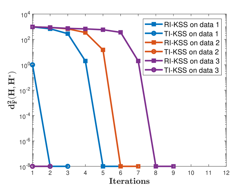
(a) $K=3$

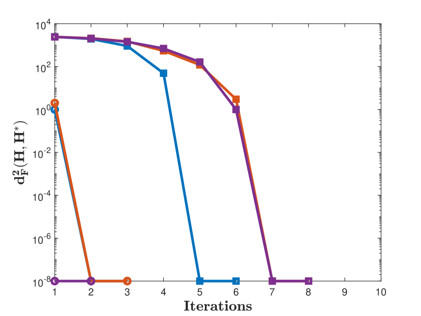
(b) $K=6$

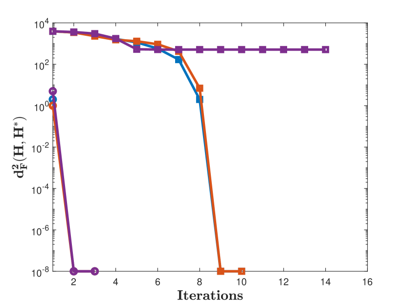
(c) $K=9$

Figure 1: Convergence performance of KSS: The $x$-axis is number of iterations and the $y$-axis is the distance from an iterate to a ground truth, i.e., $d_{F}^{2}(\bm{H}^{k},\bm{H}^{*})+10^{-8}$, where $\bm{H}^{k}$ is the $k$-th iterate generated by KSS.

In this subsection, we turn to study convergence behavior of the cluster assignment step in the KSS iterations. Observe that Problem (6) is row-separable, and thus we can solve it by dividing it into $N$ subproblems. Specifically, for a row of $\bm{G}$ denoted by $\bm{g}\in\mathbb{R}^{K}$, it suffices to consider

$$\mathcal{T}(\bm{g})=\mathop{\mathrm{arg\,min}}\left\{\langle\bm{g},\bm{h}\rangle:\bm{h}^{T}\bm{1}_{K}=1,\ \bm{h}\in\{0,1\}^{K}\right\}.$$

Then, we can show that this problem admits a closed-form solution, which may be not unique.

Lemma 5.

For any $\bm{g}\in\mathbb{R}^{K}$, it holds that $\bm{v}\in\mathcal{T}(\bm{g})$ if and only if $v_{k}=1$ and $v_{\ell}=0$ for all $\ell\neq k$, where $k\in[K]$ satisfies $g_{k}\leq g_{\ell}$ for all $\ell\neq k$. Moreover, $\bm{v}\in\mathcal{T}(\bm{g})$ if and only if $\bm{Q}\bm{v}\in\mathcal{T}(\bm{Q}\bm{g})$ for $\bm{Q}\in\Pi_{K}$.

Based on the above result, we can prove that the operator $\mathcal{T}$ possesses a Lipschitz-like property.

Lemma 6.

Suppose that $\bm{g}\in\mathbb{R}^{K}$ is arbitrary and $\delta>0$ is a constant such that $g_{\ell}-g_{k}\geq\delta$ for some $k\in[K]$ and all $\ell\neq k$. Then, for any $\bm{v}\in\mathcal{T}(\bm{g})$, $\bm{g}^{\prime}\in\mathbb{R}^{K}$, and $\bm{v}^{\prime}\in\mathcal{T}(\bm{g}^{\prime})$, it holds that

$$\|\bm{v}-\bm{v}^{\prime}\|\leq\frac{2\|\bm{g}-\bm{g}^{\prime}\|}{\delta}.$$ (40)

We are now ready to show that the number of misclassified points is bounded by the subspace distance.

Lemma 7.

Let $\pi:[K]\rightarrow[K]$ be a permutation such that $\bm{U}=\left(\bm{U}_{1},\dots,\bm{U}_{K}\right)$ with $\bm{U}_{\pi(k)}\in\mathcal{O}^{n\times d_{k}}$ for all $k\in[K]$. Suppose that $\bar{\bm{H}}\in\mathcal{T}\left(\bm{G}_{\bm{H}}(\bm{U})\right)$, where the $(i,k)$-th element of $\bm{G}_{\bm{H}}(\bm{U})\in\mathbb{R}^{N\times K}$ is $\|\bm{z}_{i}\|^{2}-\|\bm{U}_{k}^{T}\bm{z}_{i}\|^{2}$. Then, it holds for all $i\in[N]$ that

$$\|\bar{\bm{h}}_{i}-\bm{h}_{i}^{*}\bm{Q}_{\pi}\|\leq\frac{2\sqrt{\sum_{k=1}^{K}d(\bm{U}_{\pi(k)},\bm{U}_{k}^{*})}}{1-\max_{\ell\neq I_{i}}\|\bm{U}_{\ell}^{*^{T}}\bm{z}_{i}\|^{2}},$$ (41)

where the row vectors $\bar{\bm{h}}_{i},\bm{h}_{i}^{*}\in\mathbb{R}^{K}$ respectively denote the $i$-th row of $\bar{\bm{H}}$ and $\bm{H}^{*}$, and $I_{i}\in[K]$ satisfies $h_{iI_{i}}^{*}=1$ for all $i\in[N]$.

The following lemma indicates that the KSS iterations directly converge to ground truth once the distance from the current iterate to ground truth is small enough. This implies finite termination of the KKS method.

Lemma 8.

Suppose that Assumption 1 holds, $N_{\min}\gtrsim d_{k}\gtrsim\log N$ for all $k\in[K]$, and $\bm{H}^{t}\in\mathcal{M}^{N\times K}$ satisfies

$$d^{2}_{F}(\bm{H}^{t},\bm{H}^{*})\leq 2K^{2}(c_{1}+1)c_{1}d_{\min},$$ (42)

where $c_{1}$ is the constant in Lemma 3. Then, it holds with probability at least $1-2K/(d_{\min}^{2}N)-5K^{2}/N$ that

$$\bm{H}^{t+1}=\bm{H}^{*}\bm{Q}_{\pi}$$

for some $\bm{Q}_{\pi}\in\Pi_{K}$.

Equipped with the results in Sections 3.2 and 3.3, we can prove Theorem 1. The complete proof can be found in Section D.5 of the appendix.

4 Experiment Results

In this section, we report the convergence behavior, recovery performance, and numerical efficiency of the KSS method for SC on both synthetic and real datasets. All of our experiments are implemented in MATLAB R2020a on the Great Lakes HPC Cluster of the University of Michigan with 180GB memory and 16 cores. Our code is available at https://github.com/peng8wang/ICML2022-K-Subspaces.

4.1 Convergence Behavior and Recovery Performance

We first conduct 3 sets of numerical tests, which correspond to $K\in\{3,6,9\}$, to examine the convergence behavior and recovery performance of the KSS method in the semi-random UoS model (see Definition 2). We generate $K$ overlapping subspaces as follows. First, we set $n=300$, $\overline{d}=30$, $\underline{d}=25$, and uniformly at random select $d_{k}\in[\underline{d},\overline{d}]$ for all $k\in[K]$. Second, we arbitrarily generate an orthogonal matrix $\bm{U}=\left[\bm{u}_{1},\dots,\bm{u}_{n}\right]\in\mathcal{O}^{n}$ and set the shared basis as $\bar{\bm{U}}=\left[\bm{u}_{n-s+1},\dots,\bm{u}_{n}\right]$ for an integer $s\in[0,\underline{d}]$. Next, we generate $\bm{V}_{k}$ by randomly picking up $(d_{k}-s)$ columns, which are not repeated, from the first $n-s$ columns of $\bm{U}$. Finally, we form $\bm{U}_{k}^{*}=\left[\bm{V}_{k}\ \bar{\bm{U}}\right]$ for all $k\in[K]$, which ensures that the intersection between $S_{k}$ and $S_{\ell}$ is at least of dimension $s$ for all $1\leq k\neq\ell\leq K$. In each test, we generate 3 datasets by setting $s=6$ and $N_{k}=500$ for all $k\in[K]$ and respectively run the KSS method with random initialization (denoted by RI-KSS) and TIPS initialization (denoted by TI-KSS) by setting $\tau=2/\sqrt{\overline{d}}$ on them. Then, we plot the distance of the iterates to ground truth, i.e., $d_{F}^{2}(\bm{H}^{k},\bm{H}^{*})+10^{-8}$, against the iteration numbers in Figure 1. It can be observed that with a proper initialization, the KSS method converges so quickly that it finds the correct clustering within 10 iterations. This supports the result in Theorem 1. Additionally, it exhibits a finite termination phenomenon that corroborates the result in Lemma 8. Moreover, it is observed in Figure 1(c) that RI-KSS gets stuck at a local minimum while TI-KSS does not on data 3.

Table 2: Average CPU time (in seconds) and the best clustering accuracy of the tested methods on real datasets.

Accuracy	COIL100	YaleB	USPS	MNIST
KSS	0.8117	0.7154	0.8172	0.9780
SSC	0.6732	0.8277	0.6583	–
OMP	0.3393	0.8268	0.2109	0.5749
TSC	0.7343	0.4878	0.6693	0.8514
GSC	0.6550	0.7071	0.9522	0.6306
LRR	0.5500	0.6828	0.7129	–
LRSSC	0.5200	0.7088	0.6443	–
Time (s)	COIL100	YaleB	USPS	MNIST
KSS	53.53	6.90	8.85	30.53
SSC	912.25	136.36	1217.88	–
OMP	12.12	1.02	31.12	398.37
TSC	29.78	3.06	2.66	154.46
GSC	178.15	24.22	105.59	1800.00
LRR	144.25	63.31	112.56	–
LRSSC	1800.00	444.28	1800.00	–
“–” denotes out of memory.

4.2 Numerical Efficiency and Accuracy on Real Data

We now conduct experiments to examine the computational efficiency and recovery accuracy of the KSS method on real datasets. We also compare it with several state-of-the-art methods: SSC in Elhamifar & Vidal (2013), SSC solved by OMP in You et al. (2016), TSC in Heckel & Bölcskei (2015), GSC in Park et al. (2014), LRR in Liu et al. (2012), and LRSSC in Wang et al. (2019). In the implementations of SSC, OMP, LRR, and LRSSC, we use the source codes provided by their authors. We use the real datasets COIL-100 (S. A. Nene & Murase, 1996a), the cropped extended Yale B (Georghiades et al., 2001), USPS (Hull, 1994), and MNIST (LeCun, 1998). The stopping criteria for the tested methods are given as follows. For KSS, we terminate it when the norm of two consecutive iterates is less than $10^{-2}$. For SSC, LRR, and LRSSC, we use the stopping criteria in their source codes. No stopping criterion is needed for TSC and GSC due to their one-shot nature. We set the maximum iteration number of KSS, SSC, LRR, and LRSSC as 200. We set the maximum running time of all tested algorithms as 1800 seconds. For the implementation of KSS, we used the TIPS initialization except for on MNIST, where we use random initialization in Algorithm 1. More details, including data processing, parameter settings, and test results, can be found in Section F of the appendix. Then, we run each method 10 times. Note that if the algorithms are initialized deterministically, the only randomness is from the initialization for k-means in spectral clustering. To compare the computational efficiency and recovery accuracy of the tested methods, we report the average running time and best clustering accuracy for all runs of each method in Table 2. More experiment results can be also found in Section F of the appendix. It can be observed that the KSS method is in the top three in terms of both accuracy and computational efficiency for every dataset. This demonstrates the efficiency and efficacy of the KSS method for SC.

5 Concluding Remarks

In this work, we analyzed the KSS method for subspace clustering and provided a TIPS method for its initialization in the semi-random UoS model. We showed that provided an initial assignment satisfying a partial recovery condition, the KSS method converges superlinearly and achieves correct clustering within $\Theta(\log\log N)$ iterations, even when the normalized affinity between pairwise subspaces is $O(1)$. Moreover, we proved that the proposed initialization method can return a qualified initial point. All these results are demonstrated by the numerical results. A natural future direction is to study the convergence behavior and recovery performance of the KSS method in the noisy UoS model; see, e.g., Heckel & Bölcskei (2015); Soltanolkotabi et al. (2014); Tschannen & Bölcskei (2018); Wang & Xu (2013).

Appendix

 

In the appendix, we provide proofs of the technical results presented in Sections 2 and 3. To proceed, we introduce some further notations. Given a vector $\bm{a}\in\mathbb{R}^{n}$, we denote by $\mathrm{diag}(\bm{a})\in\mathbb{R}^{n\times n}$ the diagonal matrix with $\bm{a}$ on its diagonal. Given a symmetric matrix $\bm{A}$, we use $\lambda_{\min}(\bm{A})$ to denote its smallest eigenvalue. We respectively use $\bm{1}_{n}$, $\bm{E}_{n}$, and $\bm{I}_{d}$ to denote the $n$-dimensional all-one vector, $n\times n$ all-one matrix, and $d\times d$ identity matrix, and simply write $\bm{1}$, $\bm{E}$, and $\bm{I}$ when their dimension can be inferred from the context. Given two random variables $X$ and $Y$, we write $X\overset{d}{=}Y$ if $X$ and $Y$ are equal in distribution. We use $\bm{e}_{i}$ to denote a standard basis with a 1 in the $i$-th coordinate and $0$’s elsewhere. For a vector $\bm{x}\in\mathbb{R}^{n}$, we denote by $\bm{x}_{S}$ its subvector consisting of the elements indexed by the set $S$. We denote the cumulative distribution function of the standard normal distribution by

$$\Phi(x)=\frac{1}{\sqrt{2\pi}}\int_{-\infty}^{x}e^{-\frac{t^{2}}{2}}dt.$$

For any random vector $\bm{a}\sim\mathrm{Unif}(\mathbb{S}^{d-1})$, it is known that there exists a standard normal random vector such that $\bm{a}$ is its normalization. We denote such vector by $\bar{\bm{a}}$. Thus, it holds that

$$\bar{\bm{a}}\sim\mathcal{N}(\bm{0},\bm{I}_{d}),\ \bm{a}=\frac{\bar{\bm{a}}}{\|\bar{\bm{a}}\|}.$$ (43)

Moreover, let

$$\bm{U}^{*^{T}}_{k}\bm{U}^{*}_{\ell}=\bm{U}^{*}_{k\ell}\bm{\Sigma}^{*}_{k\ell}\bm{V}_{k\ell}^{*^{T}}$$ (44)

be a singular value decomposition (SVD) of $\bm{U}^{*^{T}}_{k}\bm{U}^{*}_{\ell}$, where $\sigma_{k\ell}^{(1)}\geq\dots\geq\sigma_{k\ell}^{(\min\{d_{k},d_{\ell}\})}\geq 0$ are the singular values of $\bm{U}^{*^{T}}_{k}\bm{U}^{*}_{\ell}$ and $\bm{U}^{*}_{k\ell}\in\mathcal{O}^{d_{k}},\bm{V}^{*}_{k\ell}\in\mathcal{O}^{d_{\ell}}$. Suppose that $d_{k}\geq d_{\ell}$. We have

$$\bm{U}^{*^{T}}_{k}\bm{U}^{*}_{\ell}=\bm{U}^{*}_{k\ell}\begin{bmatrix}\bar{\bm{\Sigma}}_{k\ell}^{*}\\ \bm{0}\end{bmatrix}\bm{V}_{k\ell}^{*^{T}},$$ (45)

where $\bar{\bm{\Sigma}}_{k\ell}^{*}=\mathrm{diag}\left(\sigma_{k\ell}^{(1)},\dots,\sigma_{k\ell}^{(d_{\ell})}\right)$. Suppose to the contrary that $d_{k}<d_{\ell}$. Then, we have

$$\bm{U}^{*^{T}}_{k}\bm{U}^{*}_{\ell}=\bm{U}^{*}_{k\ell}\begin{bmatrix}\bar{\bm{\Sigma}}_{k\ell}^{*}&\bm{0}\end{bmatrix}\bm{V}_{k\ell}^{*^{T}},$$ (46)

where $\bar{\bm{\Sigma}}_{k\ell}^{*}=\mathrm{diag}\left(\sigma_{k\ell}^{(1)},\dots,\sigma_{k\ell}^{(d_{k})}\right)$. According to (13) and (44), one can verify that

$$\mathrm{aff}(S_{k}^{*},S_{\ell}^{*})=\|\bm{\Sigma}_{k\ell}^{*}\|_{F}.$$ (47)

Recall that for any $\bm{U},\bm{V}\in\mathcal{O}^{n\times d}$, we use $d(\bm{U},\bm{V})=\left\|\bm{U}\bm{U}^{T}-\bm{V}\bm{V}^{T}\right\|$ to denote the distance between the subspaces respectively spanned by $\bm{U}$ and $\bm{V}$. Then, one can verify

$$d(\bm{U},\bm{V})=\left\|(\bm{I}-\bm{U}\bm{U}^{T})\bm{V}\right\|=\left\|(\bm{I}-\bm{V}\bm{V}^{T})\bm{U}\right\|=\sqrt{1-\sigma^{2}_{\min}(\bm{U}^{T}\bm{V})}.$$ (48)

Appendix A Concentration Inequalities

In this section, we present some concentration inequalities for random vectors. These inequalities play an important role in the analysis of the proposed method. We first introduce a spectral bound on the covariance estimation for random vectors generated by a uniform distribution over the sphere. It is a direct consequence of Vershynin (2018, Theorem 4.7.1) and thus we omit its proof.

Lemma 9.

Suppose that $\bm{a}_{1},\dots,\bm{a}_{m}\in\mathbb{R}^{d}$ are i.i.d. uniformly distributed over the unit sphere. Then, it holds with probability at least $1-2e^{-u}$ that

$$\left\|\frac{1}{m}\sum_{i=1}^{m}\bm{a}_{i}\bm{a}_{i}^{T}-\frac{1}{d}\bm{I}_{d}\right\|\leq\frac{c_{1}}{d}\left(\sqrt{\frac{d+u}{m}}+\frac{d+u}{m}\right),$$

where $c_{1}>0$ is an absolute constant.

We next present a bound on the deviation of the weighted sum of standard normal random variables from its mean. This is an extension of Li & Gu (2019, Lemma 7).

Lemma 10.

Let $\bm{x}\in\mathbb{R}^{d}$ be a normal random vector such that $\bm{x}\sim\mathcal{N}(\bm{0},\sigma^{2}\bm{I}_{d})$. It holds for $\lambda_{1},\dots,\lambda_{d}\in[0,1]$ with $\sum_{i=1}^{d}\lambda_{i}^{2}\geq 4$ and $t>0$ that

$$\mathbb{P}\left(\left|\sqrt{\sum_{i=1}^{d}\lambda_{i}^{2}x_{i}^{2}}-\sigma\sqrt{\sum_{i=1}^{d}\lambda_{i}^{2}}\right|\geq t+2\sigma\right)\leq 2\exp\left(-\frac{t^{2}}{2\sigma^{2}}\right).$$

Proof of Lemma 10.

We define

$$f(\bm{x})=\sqrt{\sum_{i=1}^{d}\lambda_{i}^{2}x_{i}^{2}}.$$

By calculation, we obtain

$$\|\nabla f(\bm{x})\|=\sqrt{\frac{\sum_{i=1}^{d}\lambda_{i}^{4}x_{i}^{2}}{\sum_{i=1}^{d}\lambda_{i}^{2}x_{i}^{2}}}\leq 1.$$

Applying the concentration inequality for Lipschitz functions (see, e.g., Li & Gu (2019, Lemma 6))) to $f(\bm{x})$ yields that

$$\mathbb{P}\left(\left|f(\bm{x})-\mathbb{E}[f(\bm{x})]\right|\geq t\right)\leq 2\exp\left(-\frac{t^{2}}{2\sigma^{2}}\right).$$ (49)

We first note that

$$\mathbb{E}[f(\bm{x})]\leq\sqrt{\mathbb{E}[f^{2}(\bm{x})]}=\sqrt{\mathbb{E}\left[\sum_{i=1}^{d}\lambda_{i}^{2}x_{i}^{2}\right]}=\sigma\sqrt{\sum_{i=1}^{d}\lambda_{i}^{2}}.$$ (50)

By letting $X=f(\bm{x})\geq 0$ and $\mu=\mathbb{E}[X]$, we can compute

$$\mathrm{Var}\left(X\right) =\mathbb{E}\left[(X-\mu)^{2}\right]=\int_{0}^{\infty}t^{2}d\mathbb{P}\left(\left|X-\mu\right|\leq t\right)=-\int_{0}^{\infty}t^{2}d\mathbb{P}\left(\left|X-\mu\right|>t\right)$$

$$=\int_{0}^{\infty}2t\mathbb{P}\left(\left|X-\mu\right|>t\right)dt\leq\int_{0}^{\infty}4t\exp\left(-\frac{t^{2}}{2\sigma^{2}}\right)dt=4\sigma^{2},$$

where the forth equality and the last one follow from integration by parts and the inequality is due to (49). Thus, we have

$$\mathbb{E}^{2}[f(\bm{x})] =\mathbb{E}[f^{2}(\bm{x})]-\mathrm{Var}\left(f(\bm{x})\right)=\mathbb{E}\left[\sum_{i=1}^{d}\lambda_{i}^{2}x_{i}^{2}\right]-\mathrm{Var}\left(f(\bm{x})\right)\geq\sigma^{2}\left(\sum_{i=1}^{d}\lambda_{i}^{2}-4\right).$$

This, together with $\sum_{i=1}^{d}\lambda_{i}^{2}\geq 4$, implies

$$\mathbb{E}[f(\bm{x})]\geq\sigma\sqrt{\sum_{i=1}^{d}\lambda_{i}^{2}-4}\geq\sigma\left(\sqrt{\sum_{i=1}^{d}\lambda_{i}^{2}}-2\right).$$ (51)

Plugging (50) and (51) into (49) yields the desired result. ∎

Equipped with the above results, we are ready to present a lemma that characterizes the properties of a uniform distribution over the sphere. This plays an important role in the subsequent analysis.

Lemma 11.

Suppose that $\|\bm{\Sigma}_{k\ell}^{*}\|_{F}\geq 2$ for all $1\leq k\neq\ell\leq K$ and $\bm{a}_{i}\overset{i.i.d.}{\sim}\mathrm{Unif}(\mathbb{S}^{d_{\ell}-1})$ for all $i\in[N]$. Then, it holds with probability at least $1-4N^{-2}$ that for some $i\in[N]$ and $1\leq k\neq\ell\leq K$,

$$\left|\|\bar{\bm{a}}_{i}\|-\sqrt{d_{\ell}}\right|\leq\alpha,\quad\left|\|\bm{\Sigma}^{*}_{k\ell}\bar{\bm{a}}_{i}\|-\|\bm{\Sigma}^{*}_{k\ell}\|_{F}\right|\leq\alpha,$$ (52)

and

$$\frac{\|\bm{\Sigma}^{*}_{k\ell}\|_{F}-\alpha}{\sqrt{d_{\ell}}+\alpha}\leq\|\bm{\Sigma}^{*}_{k\ell}\bm{a}_{i}\|\leq\frac{\|\bm{\Sigma}^{*}_{k\ell}\|_{F}+\alpha}{\sqrt{d_{\ell}}-\alpha},$$ (53)

where $\alpha=2\sqrt{\log N}+2$.

Proof of Lemma 11.

We first prove (52). Applying Lemma 10 with $t=2\sqrt{\log N}$ and $\lambda_{j}=1$ for all $j\in[d_{\ell}]$ to $\bar{\bm{a}}_{i}\sim\mathcal{N}(\bm{0},\bm{I}_{d_{\ell}})$ yields that

$$\mathbb{P}\left(\left|\|\bar{\bm{a}}_{i}\|-\sqrt{d_{\ell}}\right|\geq\alpha\right)\leq 2N^{-2}.$$ (54)

Suppose that $d_{k}\geq d_{\ell}$. According to (45), we have $\bm{\Sigma}_{k\ell}^{*}=\begin{bmatrix}\bar{\bm{\Sigma}}_{k\ell}^{*}\\ \bm{0}\end{bmatrix}$. Applying Lemma 10 with $t=2\sqrt{\log N}$ and $\lambda_{j}=\sigma_{k\ell}^{(j)}$ for all $j\in[d_{\ell}]$ to $\bar{\bm{a}}_{i}\sim\mathcal{N}(\bm{0},\bm{I}_{d_{\ell}})$ yields

$$\mathbb{P}\left(\left|\|\bar{\bm{\Sigma}}^{*}_{k\ell}\bar{\bm{a}}_{i}\|-\|\bar{\bm{\Sigma}}^{*}_{k\ell}\|_{F}\right|\geq\alpha\right)\leq 2N^{-2}.$$

This, together with $\|\bm{\Sigma}^{*}_{k\ell}\bar{\bm{a}}_{i}\|=\|\bar{\bm{\Sigma}}^{*}_{k\ell}\bar{\bm{a}}_{i}\|$ and $\|\bm{\Sigma}^{*}_{k\ell}\|_{F}=\|\bar{\bm{\Sigma}}^{*}_{k\ell}\|_{F}$, implies

$$\mathbb{P}\left(\left|\|\bm{\Sigma}^{*}_{k\ell}\bar{\bm{a}}_{i}\|-\|\bm{\Sigma}^{*}_{k\ell}\|_{F}\right|\geq\alpha\right)\leq 2N^{-2}.$$ (55)

Suppose to the contrary that $d_{k}<d_{\ell}$. According to (46), we have $\bm{\Sigma}_{k\ell}^{*}\bar{\bm{a}}_{i}=\left(\sigma_{k\ell}^{(1)}\bar{a}_{i1},\dots,\sigma_{k\ell}^{(d_{k})}\bar{a}_{id_{k}}\right)$. Applying Lemma 10 with $t=2\sqrt{\log N}$ and $\lambda_{j}=\sigma_{k\ell}^{(j)}$ for all $j\in[d_{k}]$ to $[\bar{\bm{a}}_{i}]_{S}\sim\mathcal{N}(\bm{0},\bm{I}_{d_{k}})$ with $S=[d_{k}]$ yields

$$\mathbb{P}\left(\left|\|\bm{\Sigma}^{*}_{k\ell}\bar{\bm{a}}_{i}\|-\|\bm{\Sigma}^{*}_{k\ell}\|_{F}\right|\geq\alpha\right)\leq 2N^{-2}.$$

This, together with (54), (55), and the union bound, implies (52).

We next prove (53) using (52). Using $\bm{a}_{i}=\bar{\bm{a}}_{i}/\|\bar{\bm{a}}_{i}\|$ and (52), we have

$$\|\bm{\Sigma}^{*}_{k\ell}\bm{a}_{i}\|=\frac{\|\bm{\Sigma}^{*}_{k\ell}\bar{\bm{a}}_{i}\|}{\|\bar{\bm{a}}_{i}\|}\leq\frac{\|\bm{\Sigma}^{*}_{k\ell}\|_{F}+\alpha}{\sqrt{d_{\ell}}-\alpha}$$

and

$$\|\bm{\Sigma}^{*}_{k\ell}\bm{a}_{i}\|=\frac{\|\bm{\Sigma}^{*}_{k\ell}\bar{\bm{a}}_{i}\|}{\|\bar{\bm{a}}_{i}\|}\geq\frac{\|\bm{\Sigma}^{*}_{k\ell}\|_{F}-\alpha}{\sqrt{d_{\ell}}+\alpha}.$$

Then, we complete the proof. ∎

Then, we present a lemma that estimates the magnitudes of some crucial parameters in our analysis.

Lemma 12.

Suppose that $\bm{z}_{i}\in\mathbb{R}^{N}$ are generated according to the semi-random UoS model such that $\bm{z}_{i}\in S_{\ell}^{*}$. Then, for any $1\leq i\neq j\leq N$ and $k\in[K]$, it holds with probability at least $1-5K^{2}/N$ that

$$\frac{\mathrm{aff}(S_{k}^{*},S_{\ell}^{*})-\alpha}{\sqrt{d_{\ell}}+\alpha}\leq\|\bm{U}_{k}^{*^{T}}\bm{z}_{i}\|\leq\frac{\mathrm{aff}(S_{k}^{*},S_{\ell}^{*})+\alpha}{\sqrt{d_{\ell}}-\alpha}$$ (56)

and

$$\left|\frac{\langle\bm{U}_{k}^{*^{T}}\bm{z}_{i},\bm{U}_{k}^{*^{T}}\bm{z}_{j}\rangle}{\|\bm{U}_{k}^{*^{T}}\bm{z}_{j}\|}\right|\leq\frac{2\sqrt{\log N}}{\sqrt{d_{\ell}}-\alpha},$$ (57)

where $\alpha=2\sqrt{\log N}+2$.

Proof of Lemma 12.

Suppose that (52) and (53) hold for all $i\in[N]$ and $k,\ell\in[K]$, which happens with probability $1-4K^{2}N^{-1}$ according to Lemma 11 and the union bound. We first show (56). Since $\bm{z}_{i}\in S_{\ell}^{*}$ and a uniform distribution over the sphere is rotationally invariant, we have $\|\bm{U}_{k}^{*^{T}}\bm{z}_{i}\|=\|\bm{U}_{k}^{*^{T}}\bm{U}_{\ell}^{*}\bm{a}_{i}\|=\|\bm{U}_{k\ell}^{*}\bm{\Sigma}^{*}_{k\ell}\bm{V}_{k\ell}^{*^{T}}\bm{a}_{i}\|\sim\|\bm{\Sigma}^{*}_{k\ell}\bm{a}_{i}\|$. This, together with (53) and (47), implies that for any $j\in[N]$ and $\ell\in[K]$,

$$\frac{\mathrm{aff}(S_{k}^{*},S_{\ell}^{*})-\alpha}{\sqrt{d_{\ell}}+\alpha}\leq\|\bm{U}_{k}^{*^{T}}\bm{z}_{i}\|\leq\frac{\mathrm{aff}(S_{k}^{*},S^{*}_{\ell})+\alpha}{\sqrt{d_{\ell}}-\alpha}.$$ (58)

We next show (57). According to $\bm{z}_{i}\in S_{\ell}^{*}$ and (43), we have

$$\frac{\langle\bm{U}_{k}^{*^{T}}\bm{z}_{i},\bm{U}_{k}^{*^{T}}\bm{z}_{j}\rangle}{\|\bm{U}_{k}^{*^{T}}\bm{z}_{j}\|}=\frac{\langle\bm{U}_{k}^{*^{T}}\bm{U}_{\ell}^{*}\bm{a}_{i},\bm{U}_{k}^{*^{T}}\bm{z}_{j}\rangle}{\|\bm{U}_{k}^{*^{T}}\bm{z}_{j}\|}=\frac{\langle\bm{U}_{k}^{*^{T}}\bm{U}_{\ell}^{*}\bar{\bm{a}}_{i},\bm{U}_{k}^{*^{T}}\bm{z}_{j}\rangle}{\|\bar{\bm{a}}_{i}\|\|\bm{U}_{k}^{*^{T}}\bm{z}_{j}\|}.$$ (59)

By letting $X$ be a standard normal random variable, i.e., $X\sim N(0,1)$, we compute

$$\mathbb{P}\left(\left|\frac{\langle\bm{U}_{k}^{*^{T}}\bm{U}_{\ell}^{*}\bar{\bm{a}}_{i},\bm{U}_{k}^{*^{T}}\bm{z}_{j}\rangle}{\|\bm{U}_{k}^{*^{T}}\bm{z}_{j}\|}\right|\leq 2\sqrt{\log N}\Bigm{|}\bm{z}_{j}\right) =\mathbb{P}\left(\left|X\right|\leq\frac{2\|\bm{U}_{k}^{*^{T}}\bm{z}_{j}\|\sqrt{\log N}}{\|\bm{U}_{\ell}^{*^{T}}\bm{U}_{k}^{*}\bm{U}_{k}^{*^{T}}\bm{z}_{j}\|}\right)$$

$$\geq\mathbb{P}\left(|X|\leq 2\sqrt{\log N}\right)\geq 1-\sqrt{\frac{2}{\pi}}\frac{N^{-2}}{\sqrt{\log N}},$$

where the equality is due to $\langle\bm{U}_{k}^{*^{T}}\bm{U}_{\ell}^{*}\bar{\bm{a}}_{i},\bm{U}_{k}^{*^{T}}\bm{z}_{j}\rangle/{\|\bm{U}_{k}^{*^{T}}\bm{z}_{j}\|}\sim\mathcal{N}\left(\bm{0},\|\bm{U}_{\ell}^{*^{T}}\bm{U}_{k}^{*}\bm{U}_{k}^{*^{T}}\bm{z}_{j}\|^{2}/\|\bm{U}_{k}^{*^{T}}\bm{z}_{j}\|^{2}\right)$ and the first inequality is due to $\|\bm{U}_{\ell}^{*^{T}}\bm{U}_{k}^{*}\bm{U}_{k}^{*^{T}}\bm{z}_{j}\|\leq\|\bm{U}_{k}^{*^{T}}\bm{z}_{j}\|$. This, together with (52), (59), and the union bound, implies that it holds with probability at least $1-K^{2}N^{-1}/{\sqrt{\log N}}$ that for all $1\leq i\neq j\leq N$ and $\ell\in[K]$,

$$\frac{|\langle\bm{U}_{k}^{*^{T}}\bm{z}_{i},\bm{U}_{k}^{*^{T}}\bm{z}_{j}\rangle|}{\|\bm{U}_{k}^{*^{T}}\bm{z}_{j}\|}\leq\frac{2\sqrt{\log N}}{\sqrt{d_{\ell}}-\alpha}.$$

This, together with (58) and the union bound, implies the desired results. ∎

Appendix B Proofs in Section 3.1

According to Assumption 2, $d_{\min}\gtrsim\log^{3}N$, and $\alpha=2\sqrt{\log N}+2$, there exists an $\varepsilon\lesssim 1/\sqrt{\log N}$ such that

$$\alpha\leq\varepsilon\mathrm{aff}(S_{k}^{*},S_{\ell}^{*})\ \text{for all}\ 1\leq k\neq\ell\leq K,\quad\alpha\leq\varepsilon\sqrt{d_{k}}\ \text{for all}\ k\in[K].$$ (60)

This result shall be used in the subsequent proofs again and again.

B.1 Proof of Lemma 1

Before we prove Lemma 1, we need the following lemma to estimate the probability of the event that $\left|\langle\bm{z}_{i},\bm{z}_{j}\rangle\right|\geq\tau$ conditioned on $\bm{z}_{j}$. Recall that we denote the cumulative distribution function of the standard normal distribution by

$$\Phi(x)=\frac{1}{\sqrt{2\pi}}\int_{-\infty}^{x}e^{-\frac{t^{2}}{2}}dt.$$

Lemma 13.

Suppose that $\bm{z}_{i}\in S_{k}^{*}$ for some $k\in[K]$. Then, it holds for any $1\leq i\neq j\leq N$ that

$$2-2\Phi\left(\frac{\tau(\sqrt{d_{k}}+\alpha)}{\|\bm{U}_{k}^{*^{T}}\bm{z}_{j}\|}\right)-2N^{-2}\leq\mathbb{P}\left(\left|\langle\bm{z}_{i},\bm{z}_{j}\rangle\right|\geq\tau\Bigm{|}\bm{z}_{j}\right)\leq 2-2\Phi\left(\frac{\tau(\sqrt{d_{k}}-\alpha)}{\|\bm{U}_{k}^{*^{T}}\bm{z}_{j}\|}\right)+2N^{-2},$$ (61)

where $\alpha=2\sqrt{\log N}+2$. In particular, we have

$$\mathbb{P}\left(\left|\langle\bm{z}_{i},\bm{z}_{j}\rangle\right|\geq\frac{\|\bm{U}_{k}^{*^{T}}\bm{z}_{j}\|\sqrt{\log N}}{\sqrt{d_{k}}}\Bigm{|}\bm{z}_{j}\right)\leq\sqrt{\frac{2}{\pi}}\frac{2\sqrt{d_{k}}}{(\sqrt{d_{k}}-\alpha)\sqrt{\log N}}N^{-\frac{(\sqrt{d_{k}}-\alpha)^{2}}{2d_{k}}}+2N^{-2}.$$ (62)

Proof of Lemma 13.

According to $\bm{z}_{i}\in S_{k}^{*}$ and (43), we have

$$\mathbb{P}\left(\left|\langle\bm{z}_{i},\bm{z}_{j}\rangle\right|\geq\tau\Bigm{|}\bm{z}_{j}\right) =2\mathbb{P}\left(\langle\bm{z}_{i},\bm{z}_{j}\rangle\geq\tau\Bigm{|}\bm{z}_{j}\right)=2\mathbb{P}\left(\langle\bm{U}_{k}^{*}\bm{a}_{i},\bm{z}_{j}\rangle\geq\tau\Bigm{|}\bm{z}_{j}\right)=2\mathbb{P}\left(\langle\bar{\bm{a}}_{i},\bm{U}_{k}^{*^{T}}\bm{z}_{j}\rangle\geq\tau\|\bar{\bm{a}}_{i}\|\Bigm{|}\bm{z}_{j}\right)$$

$$\geq 2\mathbb{P}\left(\langle\bar{\bm{a}}_{i},\bm{U}_{k}^{*^{T}}\bm{z}_{j}\rangle\geq\tau(\sqrt{d_{k}}+\alpha)\Bigm{|}\bm{z}_{j}\right)-2\mathbb{P}\left(\|\bar{\bm{a}}_{i}\|\geq\sqrt{d_{k}}+\alpha\right)$$

$$\geq 2-2\Phi\left(\frac{\tau(\sqrt{d_{k}}+\alpha)}{\|\bm{U}_{k}^{*^{T}}\bm{z}_{j}\|}\right)-2N^{-2},$$

where the first inequality is due to the union bound and the fact that $\bm{a}_{i}$ is independent of $\bm{a}_{j}$ and the second inequality follows from $\langle\bar{\bm{a}}_{i},\bm{U}_{k}^{*^{T}}\bm{z}_{j}\rangle\sim\mathcal{N}(0,\|\bm{U}_{k}^{*^{T}}\bm{z}_{j}\|^{2})$ and uses (54) for $\bar{\bm{a}}_{i}\in\mathrm{Unif}\left(\mathbb{S}^{d_{k}-1}\right)$. By the same argument, we obtain

$$\mathbb{P}\left(\left|\langle\bm{z}_{i},\bm{z}_{j}\rangle\right|\geq\tau\Bigm{|}\bm{z}_{j}\right) =2\mathbb{P}\left(\langle\bar{\bm{a}}_{i},\bm{U}_{k}^{*^{T}}\bm{z}_{j}\rangle\geq\tau\|\bar{\bm{a}}_{i}\|\Bigm{|}\bm{z}_{j}\right)$$

$$\leq 2\mathbb{P}\left(\langle\bar{\bm{a}}_{i},\bm{U}_{k}^{*^{T}}\bm{z}_{j}\rangle\geq\tau(\sqrt{d_{k}}-\alpha)\Bigm{|}\bm{z}_{j}\right)+2\mathbb{P}\left(\|\bar{\bm{a}}_{i}\|\leq\sqrt{d_{k}}-\alpha\right)$$

$$\leq 2-2\Phi\left(\frac{\tau(\sqrt{d_{k}}-\alpha)}{\|\bm{U}_{k}^{*^{T}}\bm{z}_{j}\|}\right)+2N^{-2}.$$

This, together with $\tau=\|\bm{U}_{k}^{*^{T}}\bm{z}_{j}\|\sqrt{\log N}/\sqrt{d_{k}}$, yields

$$\mathbb{P}\left(\left|\langle\bm{z}_{i},\bm{z}_{j}\rangle\right|\geq\frac{\|\bm{U}_{k}^{*^{T}}\bm{z}_{j}\|\sqrt{\log N}}{\sqrt{d_{k}}}\Bigm{|}\bm{z}_{j}\right) \leq 2-2\Phi\left(\frac{\sqrt{\log N}(\sqrt{d_{k}}-\alpha)}{\sqrt{d_{k}}}\right)+2N^{-2}$$

$$\leq\sqrt{\frac{2}{\pi}}\int_{\frac{\sqrt{\log N}(\sqrt{d_{k}}-\alpha)}{\sqrt{d_{k}}}}^{\infty}\exp\left(-\frac{t}{2}\frac{\sqrt{\log N}(\sqrt{d_{k}}-\alpha)}{\sqrt{d_{k}}}\right)dt+2N^{-2}$$

$$=\sqrt{\frac{2}{\pi}}\frac{2\sqrt{d_{k}}}{(\sqrt{d_{k}}-\alpha)\sqrt{\log N}}N^{-\frac{(\sqrt{d_{k}}-\alpha)^{2}}{2d_{k}}}+2N^{-2}.$$

∎

Proof of Lemma 1.

First, we prove (27). Suppose that a pair of data points $\bm{z}_{i},\bm{z}_{j}\in S_{k}^{*}$ for some $k\in[K]$. According to (61) in Lemma 13 and $\|\bm{U}_{k}^{*^{T}}\bm{z}_{j}\|=\|\bm{a}_{j}\|=1$ due to the UoS model, we obtain

$$2-2\Phi\left(\tau(\sqrt{d_{k}}+\alpha)\right)-2N^{-2}\leq\mathbb{P}\left(\left|\langle\bm{z}_{i},\bm{z}_{j}\rangle\right|\geq\tau\Bigm{|}\bm{z}_{j}\right)\leq 2-2\Phi\left(\tau(\sqrt{d_{k}}-\alpha)\right)+2N^{-2}.$$

This, together with $p_{kk}=\mathbb{E}\left[\mathbb{P}\left(|\langle\bm{z}_{i},\bm{z}_{j}\rangle|\geq\tau\Bigm{|}\bm{z}_{j}\right)\right]$, implies

$$2-2\Phi\left(\tau(\sqrt{d_{k}}+\alpha)\right)-2N^{-2}\leq p_{kk}\leq 2-2\Phi\left(\tau(\sqrt{d_{k}}-\alpha)\right)+2N^{-2}.$$ (63)

This, together with (21), yields that for all $k\in[K]$,

$$p_{kk}-b_{kk} \leq 2\Phi\left(\tau\sqrt{d_{k}}\right)-2\Phi\left(\tau(\sqrt{d_{k}}-\alpha)\right)+2N^{-2}\leq\sqrt{\frac{2}{\pi}}\exp\left(-\frac{\tau^{2}(\sqrt{d_{k}}-\alpha)^{2}}{2}\right)\tau\alpha+2N^{-2}\lesssim\frac{1}{\log N},$$ (64)

where the last inequality is due to (22) and $d_{\min}\gtrsim\log^{3}N$. By the same argument, we have $p_{kk}-b_{kk}\gtrsim-\frac{1}{\log N}.$ This, together with (64), implies (27) for all $k=\ell$. Suppose that a pair of data points $\bm{z}_{i}\in S_{k}^{*},\bm{z}_{j}\in S_{\ell}^{*}$ for some $1\leq k\neq\ell\leq K$. Since a uniform distribution over the sphere is rotationally invariant, we have

$$\|\bm{U}_{k}^{*^{T}}\bm{z}_{j}\|=\|\bm{U}_{k}^{*^{T}}\bm{U}_{\ell}^{*}\bm{a}_{j}\|=\|\bm{U}_{k\ell}^{*}\bm{\Sigma}_{k\ell}^{*}\bm{V}_{k\ell}^{*^{T}}\bm{a}_{j}\|\sim\|\bm{\Sigma}_{k\ell}^{*}\bm{a}_{j}\|,$$

where the second equality is due to (44). This, together with (53) in Lemma 11 and (61) in Lemma 13, implies it holds with probability at least $1-2N^{-2}$ that

$$2-2\Phi\left(\frac{\tau(\sqrt{d_{k}}+\alpha)(\sqrt{d_{\ell}}+\alpha)}{\|\bm{\Sigma}^{*}_{k\ell}\|_{F}-\alpha}\right)-2N^{-2}\leq\mathbb{P}\left(\left|\langle\bm{z}_{i},\bm{z}_{j}\rangle\right|\geq\tau\Bigm{|}\bm{z}_{j}\right)\leq 2-2\Phi\left(\frac{\tau(\sqrt{d_{k}}-\alpha)(\sqrt{d_{\ell}}-\alpha)}{\|\bm{\Sigma}^{*}_{k\ell}\|_{F}+\alpha}\right)+2N^{-2}.$$

This, together with $\mathrm{aff}(S_{k}^{*},S_{\ell}^{*})=\|\bm{\Sigma}^{*}_{k\ell}\|_{F}$ and $p_{k\ell}=\mathbb{E}\left[\mathbb{P}\left(|\langle\bm{z}_{i},\bm{z}_{j}\rangle|\geq\tau\Bigm{|}\bm{z}_{j}\right)\right]$, further implies

$$2-2\Phi\left(\frac{\tau(\sqrt{d_{k}}+\alpha)(\sqrt{d_{\ell}}+\alpha)}{\mathrm{aff}(S_{k}^{*},S_{\ell}^{*})-\alpha}\right)-4N^{-2}\leq p_{k\ell}\leq 2-2\Phi\left(\frac{\tau(\sqrt{d_{k}}-\alpha)(\sqrt{d_{\ell}}-\alpha)}{\mathrm{aff}(S_{k}^{*},S_{\ell}^{*})+\alpha}\right)+4N^{-2}.$$ (65)

This, together with (21), yields that for all $1\leq k\neq\ell\leq K$,

$$p_{k\ell}-b_{k\ell} \leq 2\Phi\left(\frac{\tau\sqrt{d_{k}d_{\ell}}}{\mathrm{aff}(S_{k}^{*},S_{\ell}^{*})}\right)-2\Phi\left(\frac{\tau(\sqrt{d_{k}}-\alpha)(\sqrt{d_{\ell}}-\alpha)}{\mathrm{aff}(S_{k}^{*},S_{\ell}^{*})+\alpha}\right)+4N^{-2}$$

$$\leq\sqrt{\frac{2}{\pi}}\exp\left(-\frac{\tau^{2}(\sqrt{d_{k}}-\alpha)^{2}(\sqrt{d_{\ell}}-\alpha)^{2}}{2(\mathrm{aff}(S_{k}^{*},S_{\ell}^{*})+\alpha)^{2}}\right)\left(\frac{\tau\sqrt{d_{k}d_{\ell}}}{\mathrm{aff}(S_{k}^{*},S_{\ell}^{*})}-\frac{\tau(\sqrt{d_{k}}-\alpha)(\sqrt{d_{\ell}}-\alpha)}{\mathrm{aff}(S_{k}^{*},S_{\ell}^{*})+\alpha}\right)$$

$$\leq\sqrt{\frac{2}{\pi}}\exp\left(-\frac{(1-\varepsilon)^{4}\tau^{2}d_{\min}^{2}}{2(1+\varepsilon)^{2}\mathrm{aff}^{2}(S_{k}^{*},S_{\ell}^{*})}\right)\left(1-\frac{(1-\varepsilon)^{2}}{1+\varepsilon}\right)\frac{\tau\sqrt{d_{k}d_{\ell}}}{\mathrm{aff}(S_{k}^{*},S_{\ell}^{*})}$$

$$=\sqrt{\frac{2}{\pi}}\frac{\varepsilon(3-\varepsilon)\tau\sqrt{d_{k}d_{\ell}}}{1+\varepsilon}\exp\left(-\frac{(1-\varepsilon)^{4}\tau^{2}d_{\min}^{2}}{2(1+\varepsilon)^{2}\mathrm{aff}^{2}(S_{k}^{*},S_{\ell}^{*})}\right)\frac{1}{\mathrm{aff}(S_{k}^{*},S_{\ell}^{*})}$$

$$=\sqrt{\frac{2}{\pi}}\exp\left(-\frac{1}{2}\right)\frac{\varepsilon(3-\varepsilon)\sqrt{d_{k}d_{\ell}}}{(1-\varepsilon)^{2}d_{\min}}\lesssim\frac{d_{\max}}{d_{\min}\sqrt{\log N}},$$ (66)

where the third inequality is due to (60) and the last inequality follows from $\varepsilon\lesssim 1/\sqrt{\log N}$ and the fact that $\exp\left(-\eta x^{2}/2\right)x$ attains the maximum at $x=1/\sqrt{\eta}$ when $x\in(0,\infty)$. By the same argument, we have $p_{k\ell}-b_{k\ell}\gtrsim-\frac{d_{\max}^{3/2}}{d_{\min}^{3/2}\sqrt{\log N}}.$ This, together with (64), implies (27) for all $1\leq k\neq\ell\leq K$.

Next, we prove (28). Note that for any $1\leq k\neq\ell\leq K$,

$$(\sqrt{d_{k}}-\alpha)(\sqrt{d_{\ell}}-\alpha)-(\sqrt{d_{k}}+\alpha)\left(\mathrm{aff}(S_{k}^{*},S^{*}_{\ell})+\alpha\right) =\sqrt{d_{k}}\left(\sqrt{d_{\ell}}-\mathrm{aff}(S_{k}^{*},S^{*}_{\ell})\right)-\alpha\left(2\sqrt{d_{k}}+\sqrt{d_{\ell}}+\mathrm{aff}(S_{k}^{*},S^{*}_{\ell})\right)$$

$$\geq\sqrt{d_{k}}\left(\sqrt{d_{\ell}}-\mathrm{aff}(S_{k}^{*},S^{*}_{\ell})\right)-2\alpha\left(\sqrt{d_{k}}+\sqrt{d_{\ell}}\right)$$

$$\geq\frac{1}{10}\sqrt{d_{k}d_{\ell}},$$ (67)

where the first inequality follows from $\mathrm{aff}(S_{k}^{*},S_{\ell}^{*})\leq\sqrt{d_{\ell}}$ and the second inequality uses $\mathrm{aff}(S_{k}^{*},S_{\ell}^{*})\leq 4\sqrt{d_{\ell}}/5$ due to (15) and $d_{\min}\gtrsim\log^{3}N$. For ease of exposition, let

$$x_{k\ell}=\frac{\tau(\sqrt{d_{k}}-\alpha)(\sqrt{d_{\ell}}-\alpha)}{\mathrm{aff}(S_{k}^{*},S_{\ell}^{*})+\alpha},\quad y_{k}=\tau(\sqrt{d_{k}}+\alpha).$$

According to (B.1) and (22), we have $x_{k\ell}>y_{k}$ for any $1\leq k\neq\ell\leq K$. For all $1\leq k\neq\ell\leq K$ satisfying $\mathrm{aff}(S_{k}^{*},S_{\ell}^{*})\geq\tau(\sqrt{d_{k}}-\alpha)(\sqrt{d_{\ell}}-\alpha)/(2c)-\alpha$, we have

$$x_{k\ell}\leq 2c$$

and

$$x_{k\ell}-y_{k}\geq\frac{\tau\sqrt{d_{k}d_{\ell}}}{10\left(\mathrm{aff}(S_{k}^{*},S_{\ell}^{*})+\alpha\right)}\geq\frac{c\sqrt{d_{k}d_{\ell}}}{10\min\{\sqrt{d_{k}},\sqrt{d_{\ell}}\}\sqrt{d_{\max}}}\gtrsim\frac{\sqrt{d_{\min}}}{\sqrt{d_{\max}}},$$

where the first inequality uses (B.1) and the second inequality follows from (60) and (15). This, together with (63), (65), and $x_{k\ell}>y_{k}$, yields that for all $1\leq k\neq\ell\leq K$,

$$p_{kk}-p_{k\ell} \geq 2\left(\Phi\left(x_{k\ell}\right)-\Phi\left(y_{k}\right)\right)-6N^{-2}\geq\sqrt{\frac{2}{\pi}}\exp\left(-\frac{x_{k\ell}^{2}}{2}\right)\left(x_{k\ell}-y_{k}\right)-6N^{-2}\gtrsim\frac{\sqrt{d_{\min}}}{\sqrt{d_{\max}}}.$$ (68)

For all $1\leq k\neq\ell\leq K$ satisfying $\mathrm{aff}(S_{k}^{*},S_{\ell}^{*})<\tau(\sqrt{d_{k}}-\alpha)(\sqrt{d_{\ell}}-\alpha)/(2c)-\alpha$, we have for all $1\leq k\neq\ell\leq K$,

$$p_{kk}\geq 2-2\Phi\left(\frac{c(\sqrt{d_{k}}+\alpha)}{\sqrt{d_{\max}}}\right)-2N^{-2}\geq 2-2\Phi\left((1+\varepsilon)c\right)-2N^{-2},$$

where the first inequality is due to (63) and (22) and the second inequality uses (60), and

$$p_{k\ell} \leq 2-2\Phi\left(2c\right)+4N^{-2}.$$

Then, we have for all $1\leq k\neq\ell\leq K$,

$$p_{kk}-p_{k\ell}\geq 2\Phi\left(2c\right)-2\Phi\left((1+\varepsilon)c\right)-6N^{-2},$$

which is a constant due to the fact that $c>0$ is a constant. This, together with (68) and $d_{\min}\gtrsim\log N$, implies (28). ∎

B.2 Proof of Lemma 2

Proof.

According to (21) and (22), we have for all $1\leq k\neq\ell\leq K$,

$$b_{kk}=2-2\Phi\left(\frac{\sqrt{cd_{k}}}{\sqrt{d_{\max}}}\right)\geq 2-2\Phi(\sqrt{c})$$ (69)

and

$$b_{k\ell}=2-2\Phi\left(\frac{\sqrt{cd_{k}d_{\ell}}}{\sqrt{d_{\max}}\mathrm{aff}(S_{k}^{*},S_{\ell}^{*})}\right)\leq 2-2\Phi\left(\frac{\sqrt{cd_{\min}}}{\kappa\sqrt{d_{\max}}}\right)=2-2\Phi\left(\frac{\sqrt{c}}{\kappa\sqrt{\kappa_{d}}}\right),$$ (70)

where the inequality is due to $\mathrm{aff}(S_{k}^{*},S_{\ell}^{*})\leq\kappa\min\{\sqrt{d_{k}},\sqrt{d}_{\ell}\}$ for all $1\leq k\neq\ell\leq K$ by Assumption 2 and (15). Then, we can decompose the symmetric matrix $\bm{B}$ into $\bm{B}=\bm{B}_{1}+\bm{B}_{2}$, where

$$\bm{B}_{1}=\begin{bmatrix}\frac{b_{11}}{2}&b_{12}&\dots&b_{1K}\\ b_{12}&\frac{b_{22}}{2}&\dots&b_{2K}\\ \vdots&\vdots&\ddots&\vdots\\ b_{1K}&b_{2K}&\dots&\frac{b_{KK}}{2}\\ \end{bmatrix},\quad\bm{B}_{2}=\frac{1}{2}\begin{bmatrix}b_{11}&0&\dots&0\\ 0&b_{22}&\dots&0\\ \vdots&\vdots&\ddots&\vdots\\ 0&0&\dots&b_{KK}\\ \end{bmatrix}.$$

According to (69), (70), and (23), we can verify for all $k\in[K]$,

$$\frac{1}{2}|b_{kk}|-\left|\sum_{\ell:k\neq\ell}b_{k\ell}\right|\geq 1-\Phi(\sqrt{c})-2(K-1)\left(1-\Phi\left(\frac{\sqrt{c}}{\kappa\sqrt{\kappa_{d}}}\right)\right)\geq 0,$$

which implies that $\bm{B}_{1}$ is a symmetric diagonally dominant matrix (see Golub & Van Loan (2013, Section 4.1.1)). Using the result that a symmetric diagonally dominant matrix with real non-negative diagonal entries is positive semidefinite, we can conclude that $\bm{B}_{1}$ is positive semidefinite. On the other hand, we can see that $\bm{B}_{2}$ is a diagonal matrix with all the diagonal elements being larger than $1-\Phi(\sqrt{c})$. Then, we have

$$\min_{\|\bm{x}\|=1}\bm{x}^{T}\bm{B}\bm{x}\geq\min_{\|\bm{x}\|=1}\bm{x}^{T}\bm{B}_{1}\bm{x}+\min_{\|\bm{x}\|=1}\bm{x}^{T}\bm{B}_{2}\bm{x}=\lambda_{\min}(\bm{B}_{1})+\lambda_{\min}(\bm{B}_{2})\geq 1-\Phi(\sqrt{c}).$$

Then, we complete the proof. ∎

B.3 Proof of Proposition 1

Before we prove Proposition 1, we need estimate the covariance between the random variables $a_{ik}$ and $a_{jk}$ generated by the thresholding procedure (11) for all $1\leq i\neq j\leq N$ and $k\in[N]$.

Lemma 14.

Suppose that $\bm{z}_{i}$, $\bm{z}_{j}$, and $\bm{z}_{k}$ are different points generated according to the semi-random UoS model such that $\bm{z}_{k}\in S_{\ell}$ for some $\ell\in[K]$. Suppose in addition that Assumption 2 holds, the thresholding parameter is set as in (22), $d_{\min}\gtrsim\log N$. Then, it holds for any $1\leq i\neq j\leq N$ with probability at least $1-5K^{2}N^{-2}$ that

$$\left|\mathbb{E}[a_{ik}a_{jk}|\bm{z}_{i},\bm{z}_{j}]-\mathbb{E}[a_{ik}|\bm{z}_{i}]\mathbb{E}[a_{jk}|\bm{z}_{j}]\right|\lesssim\frac{d_{\max}}{d_{\min}\sqrt{\log N}}.$$

Proof of Lemma 14.

Suppose that (56) and (57) hold, which happens with probability at least $1-5K^{2}/N$ according to Lemma 12. To simplify the notations, let

$$\bm{v}_{i}:=\bm{U}_{\ell}^{*^{T}}\bm{z}_{i},\ \tilde{\bm{v}}_{i}:=\frac{\bm{v}_{i}}{\|\bm{v}_{i}\|},\ \text{for all}\ i\in[N].$$ (71)

Besides, for any given $\bm{v}_{i}$ and $\bm{v}_{j}$, let

$$\beta_{ij}:=\frac{\left(\tau+|\langle\bm{v}_{i},\tilde{\bm{v}}_{j}\rangle|\sqrt{\log N}/\sqrt{d_{\ell}}\right)(\sqrt{d_{\ell}}+\alpha)}{\left(\|\bm{v}_{i}\|-|\langle\bm{v}_{i},\tilde{\bm{v}}_{j}\rangle|\right)\sqrt{1-(\log N)/d_{\ell}}},\ \beta_{ij}^{\prime}:=\frac{\left(\tau-|\langle\bm{v}_{i},\tilde{\bm{v}}_{j}\rangle|\sqrt{\log N}/\sqrt{d_{\ell}}\right)(\sqrt{d_{\ell}}-\alpha)}{\|\bm{v}_{i}\|}.$$ (72)

In addition, suppose that the following inequalities hold:

$$\mathbb{E}[a_{ik}a_{jk}|\bm{z}_{i},\bm{z}_{j}] \geq\left(2-2\Phi\left(\beta_{ij}\right)-2N^{-2}\right)\mathbb{P}\left(\tau\leq|\langle\bm{z}_{j},\bm{z}_{k}\rangle|\leq\frac{\|\bm{v}_{j}\|\sqrt{\log N}}{\sqrt{d_{\ell}}}\Bigm{|}\bm{z}_{j}\right)$$ (73)

$$\mathbb{E}[a_{ik}a_{jk}|\bm{z}_{i},\bm{z}_{j}] \leq\left(2-2\Phi\left(\beta_{ij}^{\prime}\right)+2N^{-2}\right)\mathbb{P}\left(\tau\leq|\langle\bm{z}_{j},\bm{z}_{k}\rangle|\leq\frac{\|\bm{v}_{j}\|\sqrt{\log N}}{\sqrt{d_{\ell}}}\Bigm{|}\bm{z}_{j}\right)+$$

$$\quad\left(2+2N^{-2}\right)\mathbb{P}\left(\frac{\|\bm{v}_{j}\|\sqrt{\log N}}{\sqrt{d_{\ell}}}\leq|\langle\bm{z}_{j},\bm{z}_{k}\rangle|\leq 1\Bigm{|}\bm{z}_{j}\right).$$ (74)

According to Lemma 13, we obtain

$$2-2\Phi\left(\frac{\tau(\sqrt{d_{\ell}}+\alpha)}{\|\bm{v}_{i}\|}\right)-2N^{-2}\leq\mathbb{E}[a_{ik}|\bm{z}_{i}]\leq 2-2\Phi\left(\frac{\tau(\sqrt{d_{\ell}}-\alpha)}{\|\bm{v}_{i}\|}\right)+2N^{-2}.$$ (75)

This, together with (73), yields

$$\quad\mathbb{E}[a_{ik}a_{jk}|\bm{z}_{i},\bm{z}_{j}]-\mathbb{E}[a_{ik}|\bm{z}_{i}]\mathbb{E}[a_{jk}|\bm{z}_{j}]$$

$$\geq 2\left(1-\Phi\left(\beta_{ij}\right)-N^{-2}\right)\mathbb{P}\left(\tau\leq|\langle\bm{z}_{j},\bm{z}_{k}\rangle|\leq\frac{\|\bm{v}_{j}\|\sqrt{\log N}}{\sqrt{d_{\ell}}}\Bigm{|}\bm{z}_{j}\right)-2\left(1-\Phi\left(\frac{\tau(\sqrt{d_{\ell}}-\alpha)}{\|\bm{v}_{i}\|}\right)+N^{-2}\right)$$

$$\ \mathbb{P}\left(|\langle\bm{z}_{j},\bm{z}_{k}\rangle|\geq\tau\Bigm{|}\bm{z}_{j}\right)=2\left(\Phi\left(\frac{\tau(\sqrt{d_{\ell}}-\alpha)}{\|\bm{v}_{i}\|}\right)-\Phi\left(\beta_{ij}\right)-2N^{-2}\right)\mathbb{P}\left(\tau\leq|\langle\bm{z}_{j},\bm{z}_{k}\rangle|\leq\frac{\|\bm{v}_{j}\|\sqrt{\log N}}{\sqrt{d_{\ell}}}\Bigm{|}\bm{z}_{j}\right)$$

$$-2\left(1-\Phi\left(\frac{\tau(\sqrt{d_{\ell}}-\alpha)}{\|\bm{v}_{i}\|}\right)+N^{-2}\right)\mathbb{P}\left(|\langle\bm{z}_{j},\bm{z}_{k}\rangle|\geq\frac{\|\bm{v}_{j}\|\sqrt{\log N}}{\sqrt{d_{\ell}}}\Bigm{|}\bm{z}_{j}\right)\gtrsim-\frac{d_{\max}}{d_{\min}\sqrt{\log N}},$$ (76)

where the last inequality is due to Lemma 16, Lemma 13, and (22). By the similar argument, according to (74) and (75), we have

$$\mathbb{E}[a_{ik}a_{jk}|\bm{z}_{i},\bm{z}_{j}]-\mathbb{E}[a_{ik}|\bm{z}_{i}]\mathbb{E}[a_{jk}|\bm{z}_{j}] \leq 2\left(\Phi\left(\frac{\tau(\sqrt{d_{\ell}}+\alpha)}{\|\bm{v}_{i}\|}\right)-\Phi(\beta_{ij}^{\prime})+2N^{-2}\right)\mathbb{P}\left(\tau\leq|\langle\bm{z}_{j},\bm{z}_{k}\rangle|\leq\frac{\sqrt{\log N}}{\sqrt{d_{\ell}}}\Bigm{|}\bm{z}_{j}\right)$$

$$+\ 2\left(\Phi\left(\frac{\tau(\sqrt{d_{\ell}}+\alpha)}{\|\bm{v}_{i}\|}\right)+2N^{-2}\right)\mathbb{P}\left(|\langle\bm{z}_{j},\bm{z}_{k}\rangle|\geq\frac{\sqrt{\log N}}{\sqrt{d_{\ell}}}\Bigm{|}\bm{z}_{j}\right)\lesssim\frac{d_{\max}}{d_{\min}\sqrt{\log N}}.$$

According to this and (B.3), we complete the proof.

Then, the rest of the proof is devoted to proving (73) and (74). According to (11) and $\bm{z}_{k}=\bm{U}_{\ell}^{*}\bm{a}_{k}$, we have

$$\mathbb{E}[a_{ik}a_{jk}|\bm{z}_{i},\bm{z}_{j}] =\mathbb{P}\left(|\langle\bm{z}_{i},\bm{z}_{k}\rangle|\geq\tau,|\langle\bm{z}_{j},\bm{z}_{k}\rangle|\geq\tau\Bigm{|}\bm{z}_{i},\bm{z}_{j}\right)$$

$$=\int_{-\infty}^{\infty}\mathbb{P}\left(|\langle\bm{z}_{i},\bm{z}_{k}\rangle|\geq\tau,|\langle\bm{z}_{j},\bm{z}_{k}\rangle|\geq\tau\Bigm{|}|\langle\bm{z}_{j},\bm{z}_{k}\rangle|=t,\bm{z}_{i},\bm{z}_{j}\right)d\mathbb{P}\left(|\langle\bm{z}_{j},\bm{z}_{k}\rangle|\leq t\Bigm{|}\bm{z}_{j}\right)$$

$$=\int_{\tau}^{1}\mathbb{P}\left(|\langle\bm{z}_{i},\bm{z}_{k}\rangle|\geq\tau\Bigm{|}|\langle\bm{z}_{j},\bm{z}_{k}\rangle|=t,\bm{z}_{i},\bm{z}_{j}\right)d\mathbb{P}\left(|\langle\bm{z}_{j},\bm{z}_{k}\rangle|\leq t\Bigm{|}\bm{z}_{j}\right)$$

$$=\int_{\tau}^{1}\mathbb{P}\left(|\langle\bm{v}_{i},\bm{a}_{k}\rangle|\geq\tau\Bigm{|}|\langle\bm{v}_{j},\bm{a}_{k}\rangle|=t,\bm{z}_{i},\bm{z}_{j}\right)d\mathbb{P}\left(|\langle\bm{z}_{j},\bm{z}_{k}\rangle|\leq t\Bigm{|}\bm{z}_{j}\right),$$ (77)

where the second equality is due to the the law of total probability, the third equality uses $\tau\leq|\langle\bm{z}_{j},\bm{z}_{k}\rangle|\leq 1$, and the last equality follows from $\bm{v}_{i}=\bm{U}_{\ell}^{*^{T}}\bm{z}_{i}$ for all $i\in[N]$. Due to $\|\bm{a}_{k}\|=1$ and $\|\tilde{\bm{v}}_{j}\|=1$, we can decompose $\bm{a}_{k}$ into two parts that are orthogonal:

$$\bm{a}_{k}=x\tilde{\bm{v}}_{j}+\sqrt{1-x^{2}}\bm{b}_{k},$$ (78)

where $x\in\mathbb{R}$ and $\bm{b}_{k}\in\mathbb{R}^{d_{\ell}}$ satisfying $\langle\bm{b}_{k},\tilde{\bm{v}}_{j}\rangle=0$ and $\|\bm{b}_{k}\|=1$. This, together with $|\langle\bm{v}_{j},\bm{a}_{k}\rangle|=t$, implies

$$t=|x|\|\bm{v}_{j}\|.$$ (79)

Since $\|\tilde{\bm{v}}_{j}\|=1$, there exists an orthogonal matrix $\bm{U}\in\mathcal{O}^{d_{\ell}}$ such that $\bm{U}\tilde{\bm{v}}_{j}=\bm{e}_{1}$. Let

$$\tilde{\bm{b}}_{k}:=\frac{\bm{U}^{T}\bm{a}_{k}-x\bm{e}_{1}}{\sqrt{1-x^{2}}}$$ (80)

and $\bm{c}_{k}\in\mathbb{R}^{d_{\ell}-1}$ such that $\bm{c}_{k}:=(\tilde{b}_{k2},\cdots,\tilde{b}_{kd_{\ell}})$. According to Lemma 15, we obtain

$$\bm{U}\bm{b}_{k}\sim\tilde{\bm{b}}_{k}$$ (81)

such that $\tilde{b}_{k1}=0$ and $\bm{c}_{k}\sim\mathrm{Unif}(\mathbb{S}^{d_{\ell}-2})$. Besides, let

$$\bm{w}_{i}:=\bm{v}_{i}-\langle\bm{v}_{i},\tilde{\bm{v}}_{j}\rangle\tilde{\bm{v}}_{j}.$$ (82)

According to (78), we have

$$\langle\bm{v}_{i},\bm{a}_{k}\rangle =x\langle\bm{v}_{i},\tilde{\bm{v}}_{j}\rangle+\sqrt{1-x^{2}}\langle\bm{v}_{i},\bm{b}_{k}\rangle=x\langle\bm{v}_{i},\tilde{\bm{v}}_{j}\rangle+\sqrt{1-x^{2}}\langle\bm{w}_{i},\bm{b}_{k}\rangle,$$ (83)

where the second equality is due to (82) and $\langle\tilde{\bm{v}}_{j},\bm{b}_{k}\rangle=0$. According to $\langle\bm{w}_{i},\tilde{\bm{v}}_{j}\rangle=0$, we have $\langle\bm{U}^{T}\bm{w}_{i},\bm{U}\tilde{\bm{v}}_{j}\rangle=\langle\bm{U}^{T}\bm{w}_{i},\bm{e}_{1}\rangle=0$. This, together with letting $\bm{u}_{i}$ denote the $i$-th column of $\bm{U}\in\mathcal{O}^{d_{\ell}}$ and $\bm{d}_{i}:=\left(\bm{u}_{2}^{T}\bm{w}_{i},\dots,\bm{u}_{d}^{T}\bm{w}_{i}\right)\in\mathbb{R}^{d_{\ell}-1}$, we have $\bm{u}_{1}^{T}\bm{w}_{i}=0$ and $\|\bm{d}_{i}\|=\|\bm{w}_{i}\|$. It follows from this and (81) that

$$|\langle\bm{w}_{i},\bm{b}_{k}\rangle|=|\langle\bm{U}^{T}\bm{w}_{i},\bm{U}\bm{b}_{k}\rangle|\sim|\langle\bm{U}^{T}\bm{w}_{i},\tilde{\bm{b}}_{k}\rangle|=|\langle\bm{d}_{i},\bm{c}_{k}\rangle|.$$ (84)

Now, we are ready to compute the lower bound of $\mathbb{E}[a_{ik}a_{jk}|\bm{z}_{i},\bm{z}_{j}]$. According to (B.3), (79), (83), and (84), we have

$$\mathbb{P}\left(|\langle\bm{v}_{i},\bm{a}_{k}\rangle|\geq\tau\Bigm{|}\left|\langle\bm{v}_{j},\bm{a}_{k}\rangle\right|=t,\bm{z}_{i},\bm{z}_{j}\right) \geq\mathbb{P}\left(|\langle\bm{w}_{i},\bm{b}_{k}\rangle|\geq\frac{\tau+|x\langle\bm{v}_{i},\tilde{\bm{v}}_{j}\rangle|}{\sqrt{1-x^{2}}}\Bigm{|}|x|=\frac{t}{\|\bm{v}_{j}\|},\bm{z}_{i},\bm{z}_{j}\right)$$

$$=\mathbb{P}\left(|\langle\bm{d}_{i},\bm{c}_{k}\rangle|\geq\frac{\tau\|\bm{v}_{j}\|+t|\langle\bm{v}_{i},\tilde{\bm{v}}_{j}\rangle|}{\sqrt{\|\bm{v}_{j}\|^{2}-t^{2}}}\Bigm{|}\bm{z}_{i},\bm{z}_{j}\right).$$ (85)

Then, let

$$h(t):=\frac{\left(\tau\|\bm{v}_{j}\|+t|\langle\bm{v}_{i},\tilde{\bm{v}}_{j}\rangle|\right)(\sqrt{d_{\ell}}+\alpha)}{\left(\|\bm{v}_{i}\|-|\langle\bm{v}_{i},\tilde{\bm{v}}_{j}\rangle|\right)\sqrt{\|\bm{v}_{j}\|^{2}-t^{2}}}.$$

According to the argument in Lemma 13 with $\alpha=2\sqrt{\log N}+2$, $\bm{c}_{k}\sim\mathrm{Unif}(\mathbb{S}^{d_{\ell}-2})$, and $\|\bm{d}_{i}\|=\|\bm{w}_{i}\|$, we obtain

$$\mathbb{P}\left(|\langle\bm{d}_{i},\bm{c}_{k}\rangle|\geq\frac{\tau\|\bm{v}_{j}\|+t|\langle\bm{v}_{i},\tilde{\bm{v}}_{j}\rangle|}{\sqrt{\|\bm{v}_{j}\|^{2}-t^{2}}}\Bigm{|}\bm{z}_{i},\bm{z}_{j}\right) \geq 2-2\Phi\left(\frac{\left(\tau\|\bm{v}_{j}\|+t|\langle\bm{v}_{i},\tilde{\bm{v}}_{j}\rangle|\right)(\sqrt{d_{\ell}}+\alpha)}{\|\bm{w}_{i}\|\sqrt{\|\bm{v}_{j}\|^{2}-t^{2}}}\right)-2N^{-2}$$

$$\geq 2-2\Phi\left(h(t)\right)-2N^{-2},$$ (86)

where the second inequality is due to $\|\bm{w}_{i}\|\geq\|\bm{v}_{i}\|-|\langle\bm{v}_{i},\tilde{\bm{v}}_{j}\rangle|>0$ according to (82) and the triangle inequality. According to (B.3), (B.3), and (B.3), we have

$$\mathbb{E}[a_{ik}a_{jk}|\bm{z}_{i},\bm{z}_{j}] \geq\int_{\tau}^{1}\left(2-2\Phi\left(h(t)\right)-2N^{-2}\right)d\mathbb{P}\left(|\langle\bm{z}_{j},\bm{z}_{k}\rangle|\leq t\Bigm{|}\bm{z}_{j}\right)$$

$$\geq\int_{\tau}^{\frac{\|\bm{v}_{j}\|\sqrt{\log N}}{\sqrt{d_{\ell}}}}\left(2-2\Phi\left(h(t)\right)-2N^{-2}\right)d\mathbb{P}\left(|\langle\bm{z}_{j},\bm{z}_{k}\rangle|\leq t\Bigm{|}\bm{z}_{j}\right)$$

$$\geq\int_{\tau}^{\frac{\|\bm{v}_{j}\|\sqrt{\log N}}{\sqrt{d_{\ell}}}}\left(2-2\Phi\left(\beta_{ij}\right)-2N^{-2}\right)d\mathbb{P}\left(|\langle\bm{z}_{j},\bm{z}_{k}\rangle|\leq t\Bigm{|}\bm{z}_{j}\right)$$

$$=\left(2-2\Phi\left(\beta_{ij}\right)-2N^{-2}\right)\mathbb{P}\left(\tau\leq|\langle\bm{z}_{j},\bm{z}_{k}\rangle|\leq\frac{\|\bm{v}_{j}\|\sqrt{\log N}}{\sqrt{d}}\Bigm{|}\bm{z}_{j}\right),$$ (87)

where the last inequality is because $h(t)$ is an increasing function. Next, by letting

$$g(t):=\frac{\left(\tau\|\bm{v}_{j}\|-t|\langle\bm{v}_{i},\tilde{\bm{v}}_{j}\rangle|\right)(\sqrt{d_{\ell}}-\alpha)}{\|\bm{v}_{i}\|\|\bm{v}_{j}\|},$$

we can obtain the following inequality by the same argument as (B.3) and (B.3):

$$\mathbb{P}\left(|\langle\bm{v}_{i},\bm{a}_{k}\rangle|\geq\tau\Bigm{|}\langle\bm{v}_{j},\bm{a}_{k}\rangle=t,\bm{z}_{i},\bm{z}_{j}\right) \leq 2-2\Phi\left(\frac{\left(\tau\|\bm{v}_{j}\|-t|\langle\bm{v}_{i},\tilde{\bm{v}}_{j}\rangle|\right)(\sqrt{d_{\ell}}-\alpha)}{\|\bm{w}_{i}\|\sqrt{\|\bm{v}_{j}\|^{2}-t^{2}}}\right)+2N^{-2}$$

$$\leq 2-2\Phi\left(g(t)\right)+2N^{-2},$$

where the last inequality is due to $\|\bm{w}_{i}\|\leq\|\bm{v}_{i}\|$. Besides, it holds for $t\in(\tau,\|\bm{v}_{j}\|\sqrt{\log N}/\sqrt{d_{\ell}}]$ that

$$g(t)\geq\beta_{ij}^{\prime}.$$

These, together with (B.3), imply

$$\mathbb{E}[a_{ik}a_{jk}|\bm{z}_{i},\bm{z}_{j}] \leq\int_{\tau}^{1}\left(2-2\Phi\left(g(t)\right)+2N^{-2}\right)d\mathbb{P}\left(|\langle\bm{z}_{j},\bm{z}_{k}\rangle|\leq t\Bigm{|}\bm{z}_{j}\right)$$

$$=\int_{\tau}^{\frac{\|\bm{v}_{j}\|\sqrt{\log N}}{\sqrt{d_{\ell}}}}\left(2-2\Phi\left(g(t)\right)+2N^{-2}\right)d\mathbb{P}\left(|\langle\bm{z}_{j},\bm{z}_{k}\rangle|\leq t\Bigm{|}\bm{z}_{j}\right)+$$

$$\quad\int^{1}_{\frac{\|\bm{v}_{j}\|\sqrt{\log N}}{\sqrt{d_{\ell}}}}\left(2-2\Phi\left(g(t)\right)+2N^{-2}\right)d\mathbb{P}\left(|\langle\bm{z}_{j},\bm{z}_{k}\rangle|\leq t\Bigm{|}\bm{z}_{j}\right)$$

$$\leq\left(2-2\Phi\left(\beta_{ij}^{\prime}\right)+2N^{-2}\right)\mathbb{P}\left(\tau\leq|\langle\bm{z}_{j},\bm{z}_{k}\rangle|\leq\frac{\|\bm{v}_{j}\|\sqrt{\log N}}{\sqrt{d_{\ell}}}\Bigm{|}\bm{z}_{j}\right)+$$

$$\quad\left(2+2N^{-2}\right)\mathbb{P}\left(\frac{\|\bm{v}_{j}\|\sqrt{\log N}}{\sqrt{d_{\ell}}}\leq|\langle\bm{z}_{j},\bm{z}_{k}\rangle|\leq 1\Bigm{|}\bm{z}_{j}\right).$$ (88)

∎

Proof of Proposition 1.

Suppose that (56) and (57) hold, which happens with probability at least $1-5K^{2}/N$ according to Lemma 12. For ease of exposition, let $\Delta:=\bm{A}-\mathbb{E}[\bm{A}]$. Recall the definition of $p_{k}$ and $q_{k\ell}$ for $1\leq k\neq\ell\leq K$ in Lemma 1. It follows from (11) and Lemma 1 that the $(i,j)$-th element of $\bm{A}$ satisfies $a_{ij}\sim\mathbf{Bern}(p_{ij})$ such that

$$p_{ij}=\begin{cases}p_{k},&\text{if}\ \bm{z}_{i},\bm{z}_{j}\in S_{k},\\ q_{k\ell},&\text{if}\ \bm{z}_{i}\in S_{k},\ \bm{z}_{j}\in S_{\ell},\ \text{and}\ k\neq\ell.\end{cases}$$ (89)

According to (63), (22), and $d_{\min}\gtrsim\log N$, one can verify that $p_{k}\in(0,1)$ is a constant for all $k\in[K]$. According to (65) and (22), we have for $1\leq k\neq\ell\leq K$,

$$q_{k\ell} \leq 2-2\Phi\left(\frac{\max_{k\neq\ell}\mathrm{aff}(S_{k},S_{\ell})+\alpha}{\mathrm{aff}(S_{k},S_{\ell})+\alpha}\frac{(\sqrt{d_{k}}-\alpha)(\sqrt{d_{\ell}}-\alpha)}{(\sqrt{d_{\max}}-\alpha)^{2}}\right)+4N^{-2}$$

$$\leq 2-2\Phi\left(\frac{(\sqrt{d_{k}}-\alpha)(\sqrt{d_{\ell}}-\alpha)}{(\sqrt{d_{\max}}-\alpha)^{2}}\right)+4N^{-2}.$$ (90)

Now, we are devoted to bounding $\|\Delta\|^{2}=\|\Delta^{2}\|$. First, we consider the diagonal elements of $\Delta^{2}$. According to (11), we note that $a_{ij}$ for all $j\in[n]$ are mutually independent conditioned on $\bm{z}_{i}\in\mathbb{R}^{N}$. This, together with $\delta_{ij}=a_{ij}-\mathbb{E}[a_{ij}]\in\left\{1-p_{ij},-p_{ij}\right\}$ and the Hoeffding’s inequality for general bounded random variables (see, e.g., Vershynin (2018, Theorem 2.2.6)), yields that

$$\mathbb{P}\left(\left|\sum_{j=1}^{N}\left(\delta_{ij}^{2}-\mathbb{E}[\delta_{ij}^{2}]\right)\right|\geq\sqrt{N\log N}\Bigm{|}\bm{z}_{i}\right)\leq 2\exp\left(-\frac{2N\log N}{N}\right)=2N^{-2}.$$

This, together with the union bound, yields that it holds with probability at least $1-2N^{-1}$ that for all $i\in[N]$,

$$\left|\sum_{j=1}^{N}\left(\delta_{ij}^{2}-\mathbb{E}[\delta_{ij}^{2}]\right)\right|\leq\sqrt{N\log N}.$$ (91)

Due to the fact that $p_{k}\in(0,1)$ is a constant for all $k\in[K]$ and (B.3), we have for all $1\leq i<j\leq N$,

$$\mathbb{E}[\delta_{ij}^{2}]=\mathbb{E}[a_{ij}^{2}]-\mathbb{E}^{2}[a_{ij}]=p_{ij}(1-p_{ij})$$

is less than some constant. According to this and (91), it holds with probability at least $1-2N^{-1}$ that for all $i\in[N]$,

$$\left|(\Delta^{2})_{ii}\right|=\left|\sum_{j=1}^{N}\delta_{ij}^{2}\right|\leq\left|\sum_{j=1}^{N}\mathbb{E}[\delta_{ij}^{2}]\right|+\sqrt{N\log N}\lesssim N.$$ (92)

Next, we consider the off-diagonal elements of $\Delta^{2}$. According to (11), we note that $a_{ik}a_{jk}$ for all $k\neq i$ and $k\neq j$ are mutually independent conditioned on $\bm{z}_{i},\bm{z}_{j}\in\mathbb{R}^{N}$ for all $1\leq i\neq j\leq N$. This, together with $\delta_{ij}=a_{ij}-\mathbb{E}[a_{ij}]$ and the Hoeffding’s inequality for general bounded random variables (see, e.g., Vershynin (2018, Theorem 2.2.6)), yields that

$$\mathbb{P}\left(\left|\sum_{k\neq i,k\neq j}\left(\delta_{ik}\delta_{jk}-\mathbb{E}[\delta_{ik}\delta_{jk}]\right)\right|\geq\sqrt{2N\log N}\Bigm{|}\bm{z}_{i},\bm{z}_{j}\right)\leq 2\exp\left(-\frac{4N\log N}{N}\right)=2N^{-4}.$$

According to Jensen’s inequality, Lemma 14, and $\mathbb{E}[\delta_{ik}\delta_{jk}|\bm{z}_{i},\bm{z}_{j}]=\mathbb{E}[a_{ik}a_{jk}|\bm{z}_{i},\bm{z}_{j}]-\mathbb{E}[a_{ik}|\bm{z}_{i}]\mathbb{E}[a_{jk}|\bm{z}_{j}]$, we obtain for $k\neq i,k\neq j$,

$$\left|\mathbb{E}[\delta_{ik}\delta_{jk}]\right|\leq\mathbb{E}\left[\left|\mathbb{E}[\delta_{ik}\delta_{jk}|\bm{z}_{i},\bm{z}_{j}]\right|\right]\lesssim\frac{d_{\max}}{d_{\min}\sqrt{\log N}}.$$

These, together with the union bound, yields that it holds with probability at least $1-2N^{-2}$ that for all $1\leq i\neq j\leq N$,

$$\left|\sum_{k\neq i,k\neq j}\delta_{ik}\delta_{jk}\right| \leq\left|\sum_{k\neq i,k\neq j}\left(\delta_{ik}\delta_{jk}-\mathbb{E}[\delta_{ik}\delta_{jk}]\right)\right|+\left|\sum_{k\neq i,k\neq j}\mathbb{E}[\delta_{ik}\delta_{jk}]\right|\lesssim\sqrt{2N\log N}+\frac{d_{\max}N}{d_{\min}\sqrt{\log N}}.$$

As a result, it holds with probability at least $1-2N^{-2}$ that for any $1\leq i\neq j\leq N$,

$$\left|(\Delta^{2})_{ij}\right|=\left|\sum_{k=1}^{N}\delta_{ik}\delta_{jk}\right|\lesssim\frac{d_{\max}N}{d_{\min}\sqrt{\log N}},$$ (93)

Applying the union bound to (92) and (93) yields that

$$\|\Delta^{2}\|\leq\max_{i\in[N]}\left|(\Delta^{2})_{ii}\right|+\sqrt{\sum_{i\neq j}\left|(\Delta^{2})_{ij}\right|^{2}}\lesssim N+\frac{d_{\max}N^{2}}{d_{\min}\sqrt{\log N}}$$

holds with probability at least $1-6K^{2}N^{-1}$. This further implies

$$\|\Delta\|\lesssim\sqrt{\frac{d_{\max}}{d_{\min}}}\frac{N}{\sqrt[4]{\log N}}.$$

∎

B.4 Proof of Theorem 2

Proof.

Suppose that (29) holds, which happens with probability at least $1-6K^{2}N^{-1}$ according to Proposition 1. Given $\bm{z}_{i}\in S_{k}^{*}$ and $\bm{z}_{j}\in S_{\ell}^{*}$, recall that $p_{k\ell}=\mathbb{P}\left(|\langle\bm{z}_{i},\bm{z}_{j}\rangle|\geq\tau\right)$ denotes the connection probability between any pair of data points that respectively belong to the subspaces $S_{k}^{*}$ and $S_{\ell}^{*}$ for all $1\leq k,\ell\leq K$. Let $\bm{B}:=\{b_{k\ell}\}_{1\leq k,\ell\leq K}$, $\bm{C}:=\bm{H}^{*}\bm{B}\bm{H}^{*^{T}}$, $\bm{P}:=\{p_{k\ell}\}_{1\leq k,\ell\leq K}$, and $\bm{D}:=\bm{H}^{*}\bm{P}\bm{H}^{*^{T}}$, where $b_{k\ell}$ is defined in (21). In addition, let $\hat{\bm{U}},\bm{U}\in\mathbb{R}^{n\times K}$ be respectively the eigenvectors of $\bm{A}$ and $\bm{C}$ associated with the $K$ leading eigenvalues. According to (11), one can verify that

$$\mathbb{E}[\bm{A}]=\bm{D}-\mathrm{diag}(\bm{D}).$$ (94)

We claim that $\bm{C}$ is of rank $K$ and its smallest singular value is larger than $N_{\min}\gamma$, where $\gamma\geq 1-\Phi(c)$ is given in Lemma 2. Indeed, let $\bm{\Lambda}=\mathrm{diag}\left(\sqrt{N_{1}},\dots,\sqrt{N_{K}}\right)$. Then, we have

$$\bm{C}=\bm{H}^{*}\bm{\Lambda}^{-1}\bm{\Lambda}\bm{B}\bm{\Lambda}\left(\bm{H}^{*}\bm{\Lambda}^{-1}\right)^{T}.$$

One can verify that $\bm{H}^{*}\bm{\Lambda}^{-1}$ has orthonormal columns and

$$\sigma_{\min}(\bm{C})\geq\sigma_{\min}\left(\bm{\Lambda}\bm{B}\bm{\Lambda}\right)\geq\sigma_{\min}^{2}\left(\bm{\Lambda}\right)\sigma_{\min}(\bm{B})=N_{\min}\gamma.$$

According to (94) and Lemma 1, we have

$$\|\mathbb{E}[\bm{A}]-\bm{C}\| =\|\bm{D}-\bm{C}-\mathrm{diag}(\bm{D})\|\leq\|\bm{D}-\bm{C}\|+\max_{1\leq k\leq K}p_{kk}$$

$$\leq\|\bm{H}^{*}\|^{2}\|\bm{B}-\bm{P}\|+1\leq\|\bm{H}^{*^{T}}\bm{H}^{*}\|\|\bm{B}-\bm{P}\|_{F}+1\lesssim\frac{\kappa_{d}N_{\max}}{\sqrt{\log N}}.$$

This, together with (29), yields that

$$\|\bm{A}-\bm{C}\|\leq\|\bm{A}-\mathbb{E}[\bm{A}]\|+\|\mathbb{E}[\bm{A}]-\bm{C}\|\lesssim\frac{\sqrt{\kappa_{d}}N}{\sqrt[4]{\log N}},$$

where the last inequality is due to $\kappa_{d}\lesssim\sqrt{\log N}$. This, together with Lei et al. (2015, Lemma 5.1), $\gamma\geq 1-\Phi(c)$, and the fact that $\kappa_{d}$ is a constant, yields that there exists a $\bm{Q}\in\mathcal{O}^{K}$ such that

$$\|\hat{\bm{U}}-\bm{U}\bm{Q}\|_{F}\leq\frac{2\sqrt{2K}}{N_{\min}\gamma}\|\bm{A}-\bm{C}\|\lesssim\frac{\sqrt{\kappa_{d}}N}{N_{\min}\sqrt[4]{\log N}}.$$ (95)

According to Lei et al. (2015, Lemma 2.1), we have $\bm{U}=\bm{H}^{*}\bm{X}$ for some $\bm{X}\in\mathbb{R}^{K\times K}$ with $\|\bm{x}_{k}-\bm{x}_{\ell}\|=\sqrt{1/N_{k}+1/N_{\ell}}$, where $\bm{x}_{k}$ denotes $k$-th row of $\bm{X}$. By letting $\bm{X}^{\prime}=\bm{X}\bm{Q}$, we obtain

$$\bm{U}\bm{Q}=\bm{H}^{*}\bm{X}^{\prime},$$

where $\|\bm{x}_{k}^{\prime}-\bm{x}_{\ell}^{\prime}\|=\sqrt{1/N_{k}+1/N_{\ell}}$. This, together with setting $\delta_{k}=1/{\sqrt{N_{k}}}$ in Lei et al. (2015, Lemma 5.3) and (95), yields that

$$\min_{k\in[K]}N_{k}\delta_{k}^{2}=1\gtrsim\frac{\kappa_{d}N^{2}}{N^{2}_{\min}\sqrt{\log N}}\gtrsim\|\hat{\bm{U}}-\bm{U}\bm{Q}\|_{F}^{2}$$

where the first inequality is due to $\kappa_{N}^{2}\kappa_{d}\leq\sqrt{\log N}$. This implies that there exists a $\bm{Q}\in\mathcal{O}^{K}$ such that

$$\frac{\|\hat{\bm{U}}-\bm{U}\bm{Q}\|_{F}^{2}}{\delta_{k}^{2}}\lesssim N_{k},\ \text{for all}\ k\in[K].$$ (96)

Let $\bar{\bm{U}}=\bm{H}^{0}\hat{\bm{X}}$, where $(\bm{H}^{0},\hat{\bm{X}})$ is an $(1+\varepsilon)$-approximate solution to Problem (2.3). Moreover, we define $T_{k}=\left\{i\in\mathcal{C}_{k}^{*}:\bar{\bm{u}}_{k}-\bar{\bm{u}}_{\ell}\geq\delta_{k}/2\right\}$ for all $k\in[K]$, where $\bar{\bm{u}}_{i}$ denote the $i$-th row of $\bar{\bm{U}}$. According to (96) and Lei et al. (2015, Lemma 5.3), we have

$$\sum_{k=1}^{K}\frac{|T_{k}|}{N_{k}}\lesssim\|\hat{\bm{U}}-\bm{U}\bm{Q}\|_{F}^{2}\lesssim\frac{\kappa_{d}N^{2}}{N^{2}_{\min}\sqrt{\log N}}\lesssim\frac{\kappa_{d}\kappa_{N}^{2}}{\sqrt{\log N}},$$

where the second inequality is due to (95). This implies

$$\sum_{k=1}^{K}|T_{k}|\lesssim\kappa_{d}\kappa_{N}^{2}\frac{N_{\max}}{\sqrt{\log N}}$$

Note that Lei et al. (2015, Lemma 5.3) ensures that the membership is correctly recovered outside of $\cup_{k\in[K]}T_{k}$, then we have

$$d_{F}^{2}(\bm{H},\bm{H}^{*})\lesssim\kappa_{d}\kappa_{N}^{2}\frac{N_{\max}}{\sqrt{\log N}},$$

which implies (26). Then, we complete the proof. ∎

Appendix C Proofs in Section 3.2

Recall that given an $\bm{H}\in\mathcal{M}^{N\times K}$, $\mathcal{C}_{k}=\{i\in[N]:h_{ik}=1\}$, $n_{k}=|\mathcal{C}_{k}|$ for all $k\in[K]$, and $n_{k\ell}=|\mathcal{C}_{k}\cap\mathcal{C}_{\ell}^{*}|$ for all $k,\ell\in[K]$. We can verify that the number of misclassified points in $\{\mathcal{C}_{1},\dots,\mathcal{C}_{K}\}$ represented by $\bm{H}$ with respect to $\{\mathcal{C}^{*}_{1},\dots,\mathcal{C}^{*}_{K}\}$ represented by $\bm{H}^{*}$ is $\|\bm{H}-\bm{H}^{*}\bm{Q}_{\pi^{*}}\|_{F}^{2}/2,$ where $\bm{Q}_{\pi^{*}}\in\mathop{\mathrm{arg\,min}}_{\bm{Q}\in\Pi_{K}}\|\bm{H}-\bm{H}^{*}\bm{Q}\|_{F}$. Moreover, we can verify that for a permutation $\pi:[K]\rightarrow[K]$,

$$\frac{1}{2}\|\bm{H}-\bm{H}^{*}\bm{Q}_{\pi}\|_{F}^{2}=\sum_{k=1}^{K}\sum_{\ell\neq\pi^{{-1}}(k)}n_{k\ell}=\sum_{k=1}^{K}\sum_{\ell\neq\pi(k)}n_{\ell k}.$$ (97)

and

$$\sum_{\ell:\ell\neq\pi^{{-1}}(k)}n_{k\ell}=\frac{1}{2}\sum_{\ell:\ell\neq\pi^{{-1}}(k)}\sum_{i\in\mathcal{C}_{k}\cap\mathcal{C}_{\ell}^{*}}\|\bm{h}_{i}-\bm{h}_{i}^{*}\bm{Q}_{\pi}\|^{2},\ W_{k}(\bm{H})=\max\left\{\sum_{\ell:\ell\neq\pi^{-1}(k)}n_{k\ell},\sum_{\ell:\ell\neq\pi(k)}n_{\ell k}\right\},$$ (98)

where $W_{k}(\bm{H})$ is defined in (31). Using Lemma 9, we can present a spectral bound on the deviation of the sample covariance of random vectors that follow a uniform distribution over the sphere from its mean.

Corollary 1.

Suppose that $d_{k}\geq 4\log\left(Kd_{k}^{2}N\right)$ for all $k\in[K]$. For all $k,\ell\in[K]$, it holds with probability at least $1-2K/(Nd_{\min}^{2})$ that

$$\left\|\bm{\Psi}_{k\ell}-\frac{1}{d_{\ell}}\bm{I}_{d_{\ell}}\right\|\leq\frac{5c_{1}}{4d_{\ell}}\left(\sqrt{\frac{d_{\ell}}{n_{k\ell}}}+\frac{d_{\ell}}{n_{k\ell}}\right),$$ (99)

where $\bm{\Psi}_{k\ell}$ is defined in (30) and $c_{1}>0$ is an absolute constant.

Proof of Corollary 1.

Since $i\in\mathcal{C}_{\ell}^{*}$, we have $\bm{a}_{i}\in\mathrm{Unif}(\mathbb{S}^{d_{\ell}-1})$ according to the UoS model in Definition 2. Applying Lemma 9 to (30) with $u=\log\left(Kd_{\ell}^{2}N\right)$ yields that it holds with probability at least $1-2/(Kd_{\ell}^{2}N)$ that

$$\left\|\bm{\Psi}_{k\ell}-\frac{1}{d_{\ell}}\bm{I}_{d_{\ell}}\right\|\leq\frac{c_{1}}{d_{\ell}}\left(\sqrt{\frac{d_{\ell}+\log(Kd_{\ell}^{2}N)}{n_{k\ell}}}+\frac{d_{\ell}+\log(Kd_{\ell}^{2}N)}{n_{k\ell}}\right)\leq\frac{5c_{1}}{4d_{\ell}}\left(\sqrt{\frac{d_{\ell}}{n_{k\ell}}}+\frac{d_{\ell}}{n_{k\ell}}\right),$$

where the second inequality is due to $d_{\ell}\geq 4\log(Kd_{\ell}^{2}N)$. This, together with the union bound, implies the desired result. ∎

C.1 Proof of Lemma 3

Proof of Lemma 3.

Suppose that (99) holds for all $k,\ell\in[K]$, which happens with probability at least $1-2K/(Nd_{\min}^{2})$ according to $N_{k}\gtrsim d_{k}\gtrsim\log N$ and Corollary 1. According to (30) and (32), we have for all $k\in[K]$ ,

$$n_{\pi(k)k}=|\mathcal{C}_{\pi(k)}\cap\mathcal{C}_{k}^{*}|=|\mathcal{C}^{*}_{k}|-\sum_{\ell:\ell\neq{\pi(k)}}|\mathcal{C}_{\ell}\cap\mathcal{C}_{k}^{*}|=N_{k}-\sum_{\ell:\ell\neq\pi(k)}n_{\ell k}\geq N_{k}-W_{k}(\bm{H})\geq\frac{7}{8}N_{k}.$$

This, together with (99), yields that for all $k\in[K]$,

$$\left\|\bm{\Psi}_{\pi(k)k}-\frac{1}{d_{k}}\bm{I}_{d_{k}}\right\|\leq\frac{5c_{1}}{4d_{k}}\left(\sqrt{\frac{8d_{k}}{7N_{k}}}+\frac{8d_{k}}{7N_{k}}\right)\leq\frac{5c_{1}}{2d_{k}}\sqrt{\frac{8d_{k}}{7N_{k}}}\leq\frac{1}{32d_{k}},$$

where the third and last inequalities are due to $N_{k}\gtrsim d_{k}$ for all $k\in[K]$. This, together with Weyl’s inequality, yields (33). Again, applying (99) to $\bm{\Psi}_{\pi(k)\ell}$ for all $\ell\neq k$ yields

$$\left\|\bm{\Psi}_{\pi(k)\ell}-\frac{1}{d_{\ell}}\bm{I}_{d_{\ell}}\right\|\leq\frac{5c_{1}}{4d_{\ell}}\left(\sqrt{\frac{d_{\ell}}{n_{\pi(k)\ell}}}+\frac{d_{\ell}}{n_{\pi(k)\ell}}\right).$$

This, together with Weyl’s inequality, yields (34). Then, the proof is completed. ∎

C.2 Proof of Lemma 4

Proof of Lemma 4.

Suppose that (33) and (34) hold, which happens with probability at least $1-2K/({d_{\min}^{2}N})$ according to Lemma 3. Recall that

$$\bm{G}_{\bm{U}_{k}}(\bm{H})=\sum_{i=1}^{N}h_{ik}\bm{z}_{i}\bm{z}_{i}^{T}\ \text{for all}\ k\in[K].$$ (100)

It follows from $\bm{H}\in\mathcal{M}^{N\times K}$ and $\mathcal{C}_{k}=\{i\in[N]:h_{ik}=1\}$ that $h_{ik}=1$ if $i\in\mathcal{C}_{k}$ and $h_{ik}=0$ otherwise for all $i\in[N]$. Then, we note that

$$\bm{G}_{\bm{U}_{\pi(k)}}(\bm{H})=\sum_{i\in\mathcal{C}_{\pi(k)}}\bm{z}_{i}\bm{z}_{i}^{T}=\sum_{\ell=1}^{K}\sum_{i\in\mathcal{C}_{\pi(k)}\cap\mathcal{C}_{\ell}^{*}}\bm{z}_{i}\bm{z}_{i}^{T}=\sum_{\ell=1}^{K}\sum_{i\in\mathcal{C}_{\pi(k)}\cap\mathcal{C}_{\ell}^{*}}\bm{U}_{\ell}^{*}\bm{a}_{i}\bm{a}_{i}^{T}\bm{U}_{\ell}^{*^{T}}=\sum_{\ell=1}^{K}n_{{\pi(k)}\ell}\bm{U}_{\ell}^{*}\bm{\Psi}_{{\pi(k)}\ell}\bm{U}_{\ell}^{*^{T}},$$

where the third equality is due to (2) in Definition 2 and the last equality follows from (30). To simplify the notations, we define

$$\bm{A}_{\ell}=\bm{U}_{\ell}^{*}\bm{\Psi}_{{\pi(k)}\ell}\bm{U}_{\ell}^{*^{T}}\ \text{for all}\ \ell\in[K],\quad\delta_{i}=\sigma_{i}\left(\bm{G}_{\bm{U}_{\pi(k)}}(\bm{H})\right)-\sigma_{i+1}\left(\bm{G}_{\bm{U}_{\pi(k)}}(\bm{H})\right)\ \text{for all}\ i\in[d-1].$$

On one hand, it follows from (33), $\sigma_{d_{k}}\left(\bm{\Psi}_{{\pi(k)}k}\right)\leq\sigma_{d_{k}}(\bm{A}_{k})$, and $\sigma_{1}(\bm{A}_{k})\leq\sigma_{1}\left(\bm{\Psi}_{{\pi(k)}k}\right)$ that

$$\frac{31}{32d_{k}}\leq\sigma_{d_{k}}(\bm{A}_{k})\leq\dots\leq\sigma_{1}(\bm{A}_{k})\leq\frac{33}{32d_{k}}.$$ (101)

On the other hand, it follows from $\bm{U}_{k}^{*}\in\mathcal{O}^{n\times d_{k}}$ that

$$\sigma_{d_{k}+1}(\bm{A}_{k})=\dots=\sigma_{n}(\bm{A}_{k})=0.$$ (102)

According to (30), (31), and (37), we have for all $k\in[K]$,

$$n_{\pi(k)k}=|\mathcal{C}_{k}^{*}|-\sum_{\ell:\ell\neq\pi(k)}|\mathcal{C}_{\ell}\cap\mathcal{C}_{k}^{*}|\geq N_{k}-W_{k}(\bm{H})\geq\frac{7}{8}N_{k},\ \sum_{\ell:\ell\neq k}n_{\pi(k)\ell}\leq W_{\pi(k)}(\bm{H})\leq\varepsilon N_{\min}.$$ (103)

This, together with (34), yields that for all $k\in[K]$ and $\ell\neq k$,

$$n_{\pi(k)\ell}\sigma_{1}\left(\bm{\Psi}_{\pi(k)\ell}\right) \leq\frac{n_{\pi(k)\ell}}{d_{\ell}}+\frac{5c_{1}}{4}\sqrt{\frac{n_{\pi(k)\ell}}{d_{\ell}}}+\frac{5c_{1}}{4}\leq\frac{21n_{\pi(k)\ell}}{16d_{\ell}}+\frac{5c_{1}}{4}(c_{1}+1),$$ (104)

where the second inequality is due to $2\sqrt{\alpha\beta}\leq\alpha/\rho+\rho\beta$ for any $\alpha,\beta\geq 0$ and $\rho>0$. Summing up (104) for all $\ell\neq k$ yields that for all $k\in[K]$,

$$\sum_{\ell:\ell\neq k}n_{\pi(k)\ell}\sigma_{1}\left(\bm{\Psi}_{\pi(k)\ell}\right)\leq\frac{21}{16}\sum_{\ell:\ell\neq k}\frac{n_{\pi(k)\ell}}{d_{\ell}}+\frac{5c_{1}}{4}K(c_{1}+1)\leq\frac{21\varepsilon N_{\min}}{16d_{\min}}+\frac{3\varepsilon N_{k}}{16d_{\min}}\leq\frac{3\varepsilon N_{k}}{2d_{\min}},$$ (105)

where the second inequality is due to (103) and $N_{k}\gtrsim d_{k}$. We now show (38). According to $\bm{G}_{\bm{U}_{\pi(k)}}(\bm{H})=n_{\pi(k)k}\bm{A}_{k}+\sum_{\ell\neq k}n_{\pi(k)\ell}\bm{A}_{\ell}$, we have for all $i\in[d-1]$,

$$\delta_{i} =\sigma_{i}\left(\bm{G}_{\bm{U}_{\pi(k)}}(\bm{H})\right)-\sigma_{i+1}\left(n_{\pi(k)k}\bm{A}_{k}\right)+\sigma_{i+1}\left(n_{\pi(k)k}\bm{A}_{k}\right)-\sigma_{i+1}\left(\bm{G}_{\bm{U}_{\pi(k)}}(\bm{H})\right)$$

$$\leq\sigma_{i}\left(n_{\pi(k)k}\bm{A}_{k}\right)-\sigma_{i+1}\left(n_{\pi(k)k}\bm{A}_{k}\right)+2\sigma_{1}\left(\sum_{\ell:\ell\neq k}n_{\pi(k)\ell}\bm{A}_{\ell}\right),$$

$$\leq n_{\pi(k)k}\left(\sigma_{i}\left(\bm{A}_{k}\right)-\sigma_{i+1}\left(\bm{A}_{k}\right)\right)+2\sum_{\ell:\ell\neq k}n_{\pi(k)\ell}\sigma_{1}\left(\bm{\Psi}_{\pi(k)\ell}\right),$$ (106)

where the first inequality is due to Weyl’s inequality. Plugging (101), $n_{\pi(k)k}\leq N_{k}$, and (105) into (C.2) yields that for all $i=1,\dots,d_{k}-1$,

$$\delta_{i}\leq\frac{N_{k}}{16d_{k}}+\frac{3\varepsilon N_{k}}{d_{\min}}\leq\frac{7N_{k}}{16d_{k}},$$ (107)

where the second inequality is due to $\varepsilon\leq d_{\min}/(8d_{k})$. Meanwhile, plugging (102) and (105) into (C.2) yields that for all $i=d_{k}+1,\dots,d$,

$$\delta_{i}\leq\frac{3\varepsilon N_{k}}{d_{\min}}\leq\frac{3N_{k}}{8d_{k}},$$ (108)

where the second inequality is due to $\varepsilon\leq d_{\min}/(8d_{k})$. Note that $\bm{G}_{\bm{U}_{\pi(k)}}$ is a positive semidefinite matrix and satisfies

$$\sigma_{d_{k}}\left(\bm{G}_{\bm{U}_{\pi(k)}}(\bm{H})\right) \geq\sigma_{d_{k}}\left(\bm{U}_{k}^{*}n_{\pi(k)k}\bm{\Psi}_{\pi(k)k}\bm{U}_{k}^{*^{T}}\right)-\sigma_{1}\left(\sum_{\ell:\ell\neq k}\bm{U}_{\ell}^{*}n_{\pi(k)\ell}\bm{\Psi}_{\pi(k)\ell}\bm{U}_{\ell}^{*^{T}}\right)$$

$$\geq n_{{\pi(k)k}}\sigma_{d_{k}}\left(\bm{\Psi}_{\pi(k)k}\right)-\sum_{\ell:\ell\neq k}n_{\pi(k)\ell}\sigma_{1}\left(\bm{\Psi}_{\pi(k)\ell}\right),$$ (109)

where the first inequality is due to Weyl’s inequality and the second inequality follows from $\sigma_{d}(\bm{A}\bm{U}^{T})\geq\sigma_{d}(\bm{A})$, $\sigma_{1}(\bm{A}\bm{U}^{T})\leq\sigma_{1}(\bm{A})$ for $\bm{A}\in\mathbb{R}^{d\times d}$ and $\bm{U}\in\mathcal{O}^{n\times d}$, and $\sigma_{1}(\bm{B}+\bm{C})\leq\sigma_{1}(\bm{B})+\sigma_{1}(\bm{C})$ for $\bm{B},\bm{C}\in\mathbb{R}^{m\times n}$. Plugging (33), (103), and (105) into (C.2) yields for all $k\in[K]$,

$$\sigma_{d_{k}}\left(\bm{G}_{\bm{U}_{\pi(k)}}(\bm{H})\right)\geq\frac{217N_{k}}{256d_{k}}-\frac{3\varepsilon N_{k}}{2d_{\min}}\geq\frac{217N_{k}}{256d_{k}}-\frac{3N_{k}}{16d_{k}}\geq\frac{169N_{k}}{256d_{k}},$$ (110)

where the second inequality is due to $\varepsilon\leq d_{\min}/(8d_{k})$. Applying Weyl’s inequality to $\bm{G}_{\bm{U}_{\pi(k)}}(\bm{H})$ gives

$$\sigma_{d_{k}+1}\left(\bm{G}_{\bm{U}_{\pi(k)}}(\bm{H})\right)\leq n_{\pi(k)k}\sigma_{d_{k}+1}\left(\bm{A}_{k}\right)+\sigma_{1}\left(\sum_{\ell:\ell\neq k}n_{\pi(k)\ell}\bm{A}_{\ell}\right)\leq\sum_{\ell:\ell\neq k}n_{\pi(k)\ell}\sigma_{1}\left(\bm{\Psi}_{\pi(k)\ell}\right)\leq\frac{3N_{k}}{16d_{k}},$$

where the second inequality is due to (102) and the last inequality follows from (105) and $\varepsilon\leq d_{\min}/(8d_{k})$. This, together with (110), yields

$$\delta_{d_{k}}\geq\frac{169N_{k}}{256d_{k}}-\frac{3N_{k}}{16d_{k}}=\frac{121N_{k}}{256d_{k}}.$$

This, together with (35), $\lambda_{\pi(k)i}=\sigma_{i}\left(\bm{G}_{\bm{U}_{\pi(k)}}(\bm{H})\right)$ for all $i\in[d]$ due to the positive semidefiniteness of $\bm{G}_{\bm{U}_{\pi(k)}}(\bm{H})$, (107), and (108), implies (38).

We next show (4). Note that

$$\left\|(\bm{I}-\bm{U}_{k}^{*}\bm{U}_{k}^{*^{T}})\bm{G}_{\bm{U}_{\pi(k)}}(\bm{H})\right\| =\left\|\sum_{\ell:\ell\neq k}(\bm{I}-\bm{U}_{k}^{*}\bm{U}_{k}^{*^{T}})\bm{U}_{\ell}^{*}n_{\pi(k)\ell}\bm{\Psi}_{\pi(k)\ell}\bm{U}_{\ell}^{*^{T}}\right\|$$

$$\leq\sum_{\ell:\ell\neq k}n_{\pi(k)\ell}\left\|(\bm{I}-\bm{U}_{k}^{*}\bm{U}_{k}^{*^{T}})\bm{U}_{\ell}^{*}\right\|\|\bm{\Psi}_{\pi(k)\ell}\|\leq\sum_{\ell:\ell\neq k}n_{\pi(k)\ell}\sigma_{1}\left(\bm{\Psi}_{\pi(k)\ell}\right),$$ (111)

where the last inequality is due to $\left\|(\bm{I}-\bm{U}_{k}^{*}\bm{U}_{k}^{*^{T}})\bm{U}_{\ell}^{*}\right\|\leq 1$ for any $1\leq k\neq\ell\leq K$. Since $\bm{U}_{k}$ consists of eigenvectors associated with the top $\bar{d}_{k}$ eigenvalues of $\bm{G}_{\bm{U}_{k}}(\bm{H})$ that is positive semidefinite, then we have $\bm{G}_{\bm{U}_{k}}(\bm{H})\bm{U}_{k}=\bm{U}_{k}\bm{\Sigma}_{k}$ by the eigenvalue equation, where $\bm{\Sigma}_{k}$ is a diagonal matrix with the $i$-th diagonal element being $\sigma_{i}\left(\bm{G}_{\bm{U}_{k}}(\bm{H})\right)$ for all $i\in[\bar{d}_{k}]$. This, together with (110), implies $\bm{U}_{k}=\bm{G}_{\bm{U}_{k}}(\bm{H})\bm{U}_{k}\bm{\Sigma}_{k}^{-1}$ for all $k\in[K]$. According to (38), we have

$$d(\bm{U}_{\pi(k)},\bm{U}_{k}^{*}) =\left\|(\bm{I}-\bm{U}_{k}^{*}\bm{U}_{k}^{*^{T}})\bm{U}_{\pi(k)}\right\|=\left\|(\bm{I}-\bm{U}_{k}^{*}\bm{U}_{k}^{*^{T}})\bm{G}_{\bm{U}_{\pi(k)}}(\bm{H})\bm{U}_{\pi(k)}\bm{\Sigma}_{\pi(k)}^{-1}\right\|$$

$$\leq\left\|(\bm{I}-\bm{U}_{k}^{*}\bm{U}_{k}^{*^{T}})\bm{G}_{\bm{U}_{\pi(k)}}(\bm{H})\right\|\|\bm{\Sigma}_{\pi(k)}^{-1}\|\leq\frac{256d_{k}\sum_{\ell:\ell\neq k}n_{\pi(k)\ell}\sigma_{1}(\bm{\Psi}_{\pi(k)\ell})}{169N_{k}},$$ (112)

where the first equality uses (48) and the last inequality is due to (110) and (C.2). Substituting (104) into the above inequality and summing up from $k=1$ to $k=K$ yield that for all $k\in[K]$,

$$\sum_{k=1}^{K}d(\bm{U}_{\pi(k)},\bm{U}_{k}^{*}) \leq\sum_{k=1}^{K}\frac{256d_{k}}{169N_{k}}\cdot\frac{21}{16}\left(K(c_{1}+1)c_{1}+\frac{1}{d_{\min}}\sum_{\ell:\ell\neq k}n_{\pi(k)\ell}\right)$$

$$\leq\frac{2d_{\max}}{N_{\min}}\left(K^{2}(c_{1}+1)c_{1}+\frac{1}{d_{\min}}\sum_{k=1}^{K}\sum_{\ell:\ell\neq k}n_{\pi(k)\ell}\right)$$

$$\leq\frac{2d_{\max}}{N_{\min}}\left(\frac{1}{2d_{\min}}\|\bm{H}-\bm{H}^{*}\bm{Q}_{\pi}\|_{F}^{2}+K^{2}(c_{1}+1)c_{1}\right)$$

$$\leq\frac{2d_{\max}}{N_{\min}}\max\left\{\frac{1}{d_{\min}}\|\bm{H}-\bm{H}^{*}\bm{Q}_{\pi}\|_{F}^{2},2K^{2}(c_{1}+1)c_{1}\right\},$$

where the third inequality is due to (97) and $\sum_{k=1}^{K}\sum_{\ell\neq\pi^{{-1}}(k)}n_{k\ell}=\sum_{k=1}^{K}\sum_{\ell\neq k}n_{\pi(k)\ell}$. Then, we complete the proof. ∎

Appendix D Proofs in Section 3.3

D.1 Proof of Lemma 5

Proof of Lemma 5.

Note that $\bm{h}$ satisfying $\bm{h}^{T}\bm{1}_{K}=1,\ \bm{h}\in\{0,1\}^{K}$ is a vector that has exactly one $1$ and $(K-1)$ 0’s. We can see that $\mathcal{T}(\bm{g})$ is to find the minimum element of $\bm{g}$. Then, the solution follows immediately. This also implies that for $\bm{Q}\in\Pi_{K}$, $\bm{v}\in\mathcal{T}(\bm{g})$ if and only if $\bm{Q}\bm{v}\in\mathcal{T}(\bm{Q}\bm{g})$. ∎

D.2 Proof of Lemma 6

Proof of Lemma 6.

According to Lemma 5 and $g_{\ell}>g_{k}$ for a $k\in[K]$ and all $\ell\neq k$, we see that $\mathcal{T}(\bm{g})$ is a singleton and $\{\bm{v}\}=\mathcal{T}(\bm{g})$ satisfies $v_{k}=1$ and $v_{\ell}=0$ for all $\ell\neq k$. Let $\bm{g}^{\prime}\in\mathbb{R}^{K}$ be arbitrary and $\bm{v}^{\prime}\in\mathcal{T}(\bm{g}^{\prime})$. It then follows from Lemma 5 that $v^{\prime}_{k^{\prime}}=1$ and $v_{\ell^{\prime}}=0$ for some $k^{\prime}\in[K]$ and all $\ell^{\prime}\neq k^{\prime}$ satisfying $g^{\prime}_{k^{\prime}}\leq g^{\prime}_{\ell^{\prime}}$. Suppose that $k^{\prime}=k$. Then, we have $\|\bm{v}-\bm{v}^{\prime}\|=0$, and thus (40) holds trivially. Suppose to the contrary that $k^{\prime}\neq k$. Then, we have $\|\bm{v}-\bm{v}^{\prime}\|=\sqrt{2}$. Moreover, we can compute

$$\|\bm{g}-\bm{g}^{\prime}\|^{2}\geq\left(g_{k}-g^{\prime}_{k}\right)^{2}+\left(g_{k^{\prime}}-g^{\prime}_{k^{\prime}}\right)^{2}\geq\frac{1}{2}(\underbrace{g_{k}-g_{k^{\prime}}}_{\leq-\delta}+\underbrace{g^{\prime}_{k^{\prime}}-g^{\prime}_{k}}_{\leq 0})^{2}\geq\frac{1}{2}\delta^{2}.$$

This, together with $\|\bm{v}-\bm{v}^{\prime}\|=\sqrt{2}$, implies the desired result (40). ∎

D.3 Proof of Lemma 7

Proof of Lemma 7.

Let the row vectors $\bm{g}_{i},\ \bm{g}_{i}^{*}\in\mathbb{R}^{K}$ denote the $i$-th row of $\bm{G}_{\bm{H}}(\bm{U})$ and $\bm{G}_{\bm{H}}(\bm{U}^{*})$, respectively. For all $i\in[N]$, note that $I_{i}=\{k\in[K]:h_{ik}^{*}=1\}$. According to the semi-random UoS model in Definition 2, we have for all $i\in[N]$ and $\ell\neq I_{i}$,

$$g_{i\ell}^{*}-g_{iI_{i}}^{*} =\left(\|\bm{z}_{i}\|^{2}-\|\bm{U}_{\ell}^{*^{T}}\bm{z}_{i}\|^{2}\right)-\left(\|\bm{z}_{i}\|^{2}-\|\bm{U}_{I_{i}}^{*^{T}}\bm{z}_{i}\|^{2}\right)=\|\bm{U}_{I_{i}}^{*^{T}}\bm{U}_{I_{i}}^{*}\bm{a}_{i}\|^{2}-\|\bm{U}_{\ell}^{*^{T}}\bm{z}_{i}\|^{2}$$

$$=1-\|\bm{U}_{\ell}^{*^{T}}\bm{z}_{i}\|^{2}\geq 1-\max_{\ell\neq I_{i}}\|\bm{U}_{\ell}^{*^{T}}\bm{z}_{i}\|^{2},$$

where the last equality is due to $\|\bm{a}_{i}\|=1$. This, together with Lemma 5 and $\|\bm{U}_{\ell}^{*^{T}}\bm{z}_{i}\|<1$ for all $\ell\neq I_{i}$, implies

$$\{\bm{H}^{*}\}=\mathcal{T}\left(\bm{G}_{\bm{H}}(\bm{U}^{*})\right).$$ (113)

Besides, we note that for each $i\in[N]$ and $\bm{Q}_{\pi}\in\Pi_{K}$,

$$\|\bm{g}_{i}\bm{Q}_{\pi}^{T}-\bm{g}_{i}^{*}\|^{2} =\sum_{k=1}^{K}\left(\|\bm{U}_{\pi(k)}^{T}\bm{z}_{i}\|^{2}-\|\bm{U}_{k}^{*^{T}}\bm{z}_{i}\|^{2}\right)^{2}\leq\sum_{k=1}^{K}\|\bm{U}_{\pi(k)}\bm{U}_{\pi(k)}^{T}-\bm{U}_{k}^{*}\bm{U}_{k}^{*^{T}}\|^{2}\|\bm{z}_{i}\|^{4}=\sum_{k=1}^{K}d^{2}(\bm{U}_{\pi(k)},\bm{U}_{k}^{*}),$$

where the first equality is due to $\bm{g}\bm{Q}_{\pi}^{T}=\begin{bmatrix}g_{\pi(1)}&\dots&g_{\pi(K)}\end{bmatrix}$. This, together with Lemma 6 and (113), implies for all $i\in[N]$,

$$\|\bar{\bm{h}}_{i}-\bm{h}_{i}^{*}\bm{Q}_{\pi}\| =\|\bar{\bm{h}}_{i}\bm{Q}_{\pi}^{T}-\bm{h}_{i}^{*}\|\leq\frac{2\|\bm{g}_{i}\bm{Q}_{\pi}^{T}-\bm{g}_{i}^{*}\|}{1-\max_{\ell\neq I_{i}}\|\bm{U}_{\ell}^{*^{T}}\bm{z}_{i}\|^{2}}\leq\frac{2\sqrt{\sum_{k=1}^{K}d^{2}(\bm{U}_{\pi(k)},\bm{U}_{k}^{*})}}{1-\max_{\ell\neq I_{i}}\|\bm{U}_{\ell}^{*^{T}}\bm{z}_{i}\|^{2}},$$

where the first inequality uses the fact that $\bm{H}\bm{Q}^{T}\in\mathcal{T}(\bm{G}_{\bm{H}}(\bm{U})\bm{Q}^{T})$ for $\bm{Q}\in\Pi_{K}$ if and only if $\bm{H}\in\mathcal{T}(\bm{G}_{\bm{H}}(\bm{U}))$ due to Lemma 5. ∎

With the preparations in Sections 3.2 and 3.3, we can analyze each iteration of the KSS method as follows.

Proposition 2.

Let $\varepsilon\in\left(0,\frac{d_{\min}}{8d_{\max}}\right]$ be a constant. Suppose that Assumption 1 holds, $N_{\min}\gtrsim d_{k}\gtrsim\log N$ for all $k\in[K]$, and $\bm{H}^{t}\in\mathcal{M}^{N\times K}$ satisfies

$$\|\bm{H}^{t}-\bm{H}^{*}\bm{Q}_{\pi}\|_{F}^{2}\leq 2\varepsilon N_{\min},$$ (114)

where $\bm{Q}_{\pi}\in\mathop{\mathrm{arg\,min}}_{\bm{Q}\in\Pi_{K}}\|\bm{H}^{t}-\bm{H}^{*}\bm{Q}\|_{F}$. Then, it holds with probability at least $1-2K/(d_{\min}^{2}N)-5K^{2}/N$ that $\hat{d}_{\pi(k)}=d_{k}$ for all $k\in[K]$,

$$\sum_{k=1}^{K}d(\bm{U}^{t+1}_{\pi(k)},\bm{U}_{k}^{*})\leq\frac{2d_{\max}}{N_{\min}} \max\left\{\frac{1}{d_{\min}}\|\bm{H}^{t}-\bm{H}^{*}\bm{Q}_{\pi}\|_{F}^{2},2K^{2}(c_{1}+1)c_{1}\right\},$$ (115)

and for all $i\in[N]$,

$$\|\bm{h}_{i}^{t+1}-\bm{h}_{i}^{*}\bm{Q}_{\pi}\|\leq\frac{2}{1-\kappa}\sqrt{\sum_{k=1}^{K}d^{2}(\ \bm{U}_{\pi(k)}^{t+1},\bm{U}_{k}^{*})},$$ (116)

where the row vectors $\bm{h}^{t+1}_{i},\bm{h}_{i}^{*}\in\mathbb{R}^{K}$ respectively denote the $i$-th row of $\bm{H}^{t+1}$ and $\bm{H}^{*}$.

Proof of Proposition 2.

Suppose that (33), (34), and (56) hold, which happens with probability at least $1-5K^{2}/N-2K/({d_{\min}^{2}N})$ according to Lemma 3, Lemma 12,and the union bound. According to (97), we have $W_{k}(\bm{H}^{t})\leq\|\bm{H}^{t}-\bm{H}^{*}\bm{Q}_{\pi}\|_{F}^{2}/2\leq\varepsilon N_{\min}$. It follows from this and Lemma 4 that $\hat{d}^{t+1}_{\pi(k)}=d_{k}$ for all $k\in[K]$ and (115). Next, note that $I_{i}=\{k\in[K]:h_{ik}^{*}=1\}$ for all $i\in[N]$. This, together with (15) in Assumption 1 and (56), implies that for all $i\in[N]$ and $\ell\neq I_{i}$,

$$\|\bm{U}_{\ell}^{*^{T}}\bm{z}_{i}\|^{2}\leq\left(\frac{\mathrm{aff}(S_{I_{i}},S_{\ell}^{*})+\alpha}{\sqrt{d_{\ell}}-\alpha}\right)^{2}\leq\left(\frac{\kappa\sqrt{d_{\ell}}+\alpha}{\sqrt{d_{\ell}}-\alpha}\right)^{2}=\left(\kappa+\frac{(1-\kappa)\alpha}{\sqrt{d_{\ell}}-\alpha}\right)^{2}\leq 2\kappa^{2}\leq\kappa,$$ (117)

where the third inequality is due to $d_{k}\gtrsim\log N$ for all $k\in[K]$ and the last inequality is due to $\kappa\leq 1/2$. Using this and Lemma 7 yields (116). ∎

D.4 Proof of Lemma 8

Proof of Lemma 8.

Suppose that (115) and (116) hold, which happens with probability at least $1-2K/(d_{\min}^{2}N)-5K^{2}/N$ according to (42), $N_{\min}\gtrsim d_{k}$ for all $k\in[K]$, and Proposition 2. According to (42) and (115), we obtain

$$\sum_{k=1}^{K}d(\bm{U}^{t+1}_{\pi(k)},\bm{U}_{k}^{*})\leq\frac{4d_{\max}}{N_{\min}}K^{2}(c_{1}+1)c_{1}.$$

This, together with (116), $\kappa\leq 1/2$, and $N_{\min}\gtrsim d_{\max}$, yields that for all $i\in[N]$,

$$\|\bm{h}^{t+1}_{i}-\bm{h}_{i}^{*}\bm{Q}_{\pi}\|\leq 4\sum_{k=1}^{K}d(\bm{U}^{t+1}_{\pi(k)},\bm{U}_{k}^{*})\leq\frac{16d_{\max}}{N_{\min}}K^{2}(c_{1}+1)c_{1}<1.$$

Since $\bm{h}^{t+1}_{i},\bm{h}_{i}\in\{0,1\}^{K}$ for all $i\in[N]$, then we have $\bm{h}^{t+1}_{i}=\bm{h}_{i}^{*}\bm{Q}_{\pi}$ for all $i\in[N]$. Thus, $\bm{H}^{t+1}=\bm{H}^{*}\bm{Q}_{\pi}$. Moreover, due to the fact that $\min_{\bm{Q}\in\Pi_{K}}\|\bm{H}^{t+1}-\bm{H}^{*}\bm{Q}\|_{F}\leq\|\bm{H}^{t+1}-\bm{H}^{*}\bm{Q}_{\pi}\|_{F}=0$, the desired result is implied. ∎

D.5 Proof of Theorem 1

We should point out that a technical issue occurred in our analysis is that we cannot infinitely use the result in Proposition 2 infinitely due to the union bound. Then, we study $T=\Theta\left(\log\log N\right)$ iterates.

Proof of Theorem 1.

For ease of exposition, let $\pi^{t}:[K]\rightarrow[K]$ be a permutation such that

$$\bm{Q}_{\pi^{t}}\in\mathop{\mathrm{arg\,min}}_{\bm{Q}\in\Pi_{K}}\|\bm{H}^{t}-\bm{H}^{*}\bm{Q}\|_{F}$$ (118)

and the row vector $\bm{h}_{i}\in\mathbb{R}^{K}$ denote the $i$-th row of $\bm{H}\in\mathcal{M}^{N\times K}$ for all $i\in[N]$. We first show (i). Suppose that $t\leq T$ is a positive integer such that

$$\|\bm{H}^{t}-\bm{H}^{*}\bm{Q}_{\pi^{t}}\|_{F}^{2}\leq 2K^{2}(c_{1}+1)c_{1}d_{\min}.$$

Using Lemma 8, it holds with probability at least $1-2K/(d_{\min}^{2}N)-5K^{2}/N$ that

$$\bm{H}^{t+1}=\bm{H}^{*}\bm{Q}_{\pi^{t+1}}.$$

Then, it suffices to consider that for all $t\leq T$ such that

$$\|\bm{H}^{t}-\bm{H}^{*}\bm{Q}_{\pi^{t}}\|_{F}^{2}>2K^{2}(c_{1}+1)c_{1}d_{\min}.$$ (119)

We first consider $t=0$. According to (17), Proposition 2, and (119), it holds with probability at least $1-2K/(d_{\min}^{2}N)-5K^{2}/N$ that $\hat{d}^{1}_{\pi^{0}(k)}=d_{k}$ for all $k\in[K]$,

$$\sum_{k=1}^{K}d(\bm{U}^{1}_{\pi^{0}(k)},\bm{U}_{k}^{*})\leq\frac{2d_{\max}}{N_{\min}d_{\min}}\|\bm{H}^{0}-\bm{H}^{*}\bm{Q}_{\pi^{0}}\|_{F}^{2}$$ (120)

and for all $i\in[N]$,

$$\|\bm{h}_{i}^{1}-\bm{h}^{*}_{i}\bm{Q}_{\pi^{0}}\|\leq\frac{2}{1-\kappa}\sqrt{\sum_{k=1}^{K}d^{2}(\bm{U}^{1}_{\pi^{0}(k)},\bm{U}_{k}^{*})}.$$ (121)

Summing up (121) from $i=1$ to $i=N$ gives

$$\|\bm{H}^{1}-\bm{H}^{*}\bm{Q}_{\pi^{0}}\|_{F}\leq\frac{2\sqrt{N}}{1-\kappa}\sqrt{\sum_{k=1}^{K}d^{2}(\bm{U}^{1}_{\pi^{0}(k)},\bm{U}_{k}^{*})}\leq\frac{2\sqrt{N}}{1-\kappa}\sum_{k=1}^{K}d(\bm{U}^{1}_{\pi^{0}(k)},\bm{U}_{k}^{*}).$$ (122)

This, together with (120) and (17), yields that

$$\|\bm{H}^{1}-\bm{H}^{*}\bm{Q}_{\pi^{0}}\|_{F}\leq\frac{2\sqrt{N}}{1-\kappa}\frac{2d_{\max}}{N_{\min}d_{\min}}\|\bm{H}^{0}-\bm{H}^{*}\bm{Q}_{\pi^{0}}\|_{F}^{2}=\kappa_{1}\|\bm{H}^{0}-\bm{H}^{*}\bm{Q}_{\pi^{0}}\|_{F},$$ (123)

where

$$\kappa_{1}:=\frac{2\sqrt{N}}{1-\kappa}\frac{2d_{\max}}{N_{\min}d_{\min}}\|\bm{H}^{0}-\bm{H}^{*}\bm{Q}_{\pi^{0}}\|_{F}\leq\frac{2\sqrt{N}}{1-\kappa}\frac{2d_{\max}}{N_{\min}d_{\min}}\frac{(1-\kappa)d_{\min}N_{\min}}{5d_{\max}\sqrt{N}}=\frac{4}{5}.$$ (124)

Now, we use mathematical induction to show that it holds for all $t\in[T]$ that

$$\sum_{k=1}^{K}d(\bm{U}^{t+1}_{\pi^{t}(k)},\bm{U}_{k}^{*})\leq\kappa_{1}^{2^{t}}\sum_{k=1}^{K}d(\bm{U}^{t}_{\pi^{t-1}(k)},\bm{U}_{k}^{*}),$$ (125)

$$\|\bm{H}^{t+1}-\bm{H}^{*}\bm{Q}_{\pi^{t+1}}\|_{F}\leq\kappa_{1}^{2^{t}}\|\bm{H}^{t}-\bm{H}^{*}\bm{Q}_{\pi^{t}}\|_{F},$$ (126)

$$\|\bm{H}^{t}-\bm{H}^{*}\bm{Q}_{\pi^{t-1}}\|_{F}\leq\frac{2\sqrt{N}}{1-\kappa}\sum_{k=1}^{K}d(\bm{U}^{t}_{\pi^{t-1}(k)},\bm{U}_{k}^{*}).$$ (127)

We first verify (125), (126), and (127) for $t=1$. Due to (118) and (123), we obtain

$$\|\bm{H}^{1}-\bm{H}^{*}\bm{Q}_{\pi^{1}}\|_{F}\leq\|\bm{H}^{1}-\bm{H}^{*}\bm{Q}_{\pi^{0}}\|_{F}\leq\kappa_{1}\|\bm{H}^{0}-\bm{H}^{*}\bm{Q}_{\pi^{0}}\|_{F}.$$ (128)

According to this, (124), Proposition 2, and (119), it holds with probability at least $1-2K/(d_{\min}^{2}N)-5K^{2}/N$ that $\hat{d}^{2}_{\pi^{1}(k)}=d_{k}$ for all $k\in[K]$,

$$\sum_{k=1}^{K}d(\bm{U}^{2}_{\pi^{1}(k)},\bm{U}_{k}^{*})\leq\frac{2d_{\max}}{N_{\min}d_{\min}}\|\bm{H}^{1}-\bm{H}^{*}\bm{Q}_{\pi^{1}}\|_{F}^{2}$$ (129)

and for all $i\in[N]$,

$$\|\bm{h}_{i}^{2}-\bm{h}^{*}_{i}\bm{Q}_{\pi^{1}}\|\leq\frac{2}{1-\kappa}\sqrt{\sum_{k=1}^{K}d^{2}(\bm{U}^{2}_{\pi^{1}(k)},\bm{U}_{k}^{*})}.$$ (130)

Substituting (122) with the first inequality of (128) into (129) yields that

$$\sum_{k=1}^{K}d(\bm{U}^{2}_{\pi^{1}(k)},\bm{U}_{k}^{*}) \leq\frac{2d_{\max}}{N_{\min}d_{\min}}\|\bm{H}^{1}-\bm{H}^{*}\bm{Q}_{\pi^{1}}\|_{F}\cdot\frac{2\sqrt{N}}{1-\kappa}\sum_{k=1}^{K}d(\bm{U}^{1}_{\pi^{0}(k)},\bm{U}_{k}^{*})$$

$$\leq\frac{\kappa_{1}\sqrt{N}}{1-\kappa}\frac{4d_{\max}}{N_{\min}d_{\min}}\|\bm{H}^{0}-\bm{H}^{*}\bm{Q}_{\pi^{0}}\|_{F}\sum_{k=1}^{K}d(\bm{U}^{1}_{\pi^{0}(k)},\bm{U}_{k}^{*})$$

$$=\kappa_{1}^{2}\sum_{k=1}^{K}d(\bm{U}^{1}_{\pi^{0}(k)},\bm{U}_{k}^{*}),$$

where the second inequality follows from (128) and the equality is due to (124). Thus, (125) holds for $t=1$. According to (130), repeating the arguments in (122) and (123), we obtain

$$\|\bm{H}^{2}-\bm{H}^{*}\bm{Q}_{\pi^{1}}\|_{F}\leq\frac{2\sqrt{N}}{1-\kappa}\sum_{k=1}^{K}d(\bm{U}^{2}_{\pi^{1}(k)},\bm{U}_{k}^{*})$$

and

$$\|\bm{H}^{2}-\bm{H}^{*}\bm{Q}_{\pi^{1}}\|_{F} \leq\frac{2\sqrt{N}}{1-\kappa}\frac{2d_{\max}}{N_{\min}d_{\min}}\|\bm{H}^{1}-\bm{H}^{*}\bm{Q}_{\pi^{1}}\|_{F}^{2}$$

$$\leq\frac{2\sqrt{N}}{1-\kappa}\frac{2d_{\max}}{N_{\min}d_{\min}}\kappa_{1}\|\bm{H}^{0}-\bm{H}^{*}\bm{Q}_{\pi^{0}}\|_{F}\|\bm{H}^{1}-\bm{H}^{*}\bm{Q}_{\pi^{1}}\|_{F}=\kappa_{1}^{2}\|\bm{H}^{1}-\bm{H}^{*}\bm{Q}_{\pi^{1}}\|_{F},$$

where the second inequality is due to the equality in (123). This, together with (118), implies

$$\|\bm{H}^{2}-\bm{H}^{*}\bm{Q}_{\pi^{2}}\|_{F}\leq\kappa_{1}^{2}\|\bm{H}^{1}-\bm{H}^{*}\bm{Q}_{\pi^{1}}\|_{F}.$$

Thus, (127) and (126) holds for $t=1$. Next, suppose that (125), (126), and (127) hold for all $t\geq 1$. Then, we can show that (128),(129), and (130) also hold for $t+1$ using the same arguments as those of $t=1$. Consequently, we can further show that (125), (126), and (127) hold for $t+1$ until $t=T$ . Finally, we use mathematical induction and deduce that for all $t\in[T]$, the desired results (125) and (126) hold with probability at least $1-(T+1)(2K/(d_{\min}^{2}N)+5K^{2}/N)$ according to the union bound. It follows from (123) and (126) that

$$d_{F}\left(\bm{H}^{t+1},\bm{H}^{*}\right)\leq\kappa_{1}^{2^{t}}\kappa_{1}^{2^{t-1}}\dots\kappa_{1}^{2^{1}}\|\bm{H}^{1}-\bm{H}^{*}\bm{Q}_{\pi^{1}}\|_{F}\leq\kappa_{1}^{2^{t+1}-1}\|\bm{H}^{0}-\bm{H}^{*}\bm{Q}_{\pi^{0}}\|_{F}=\kappa_{1}^{2^{t+1}-1}d_{F}\left(\bm{H}^{0},\bm{H}^{*}\right).$$

We next show (ii). It follows from $T=\log_{2}\left(\frac{\log\left((1-\kappa)\sqrt{d_{\min}}N_{\min}\right)-\log(5\sqrt{2}Kc_{1}\kappa_{1}d_{\max}\sqrt{N})}{\log(1/\kappa_{1})}\right)+1$ that

$$d_{F}\left(\bm{H}^{T-1},\bm{H}^{*}\right) \leq\kappa_{1}^{2^{T-1}}\frac{(1-\kappa)d_{\min}N_{\min}}{5\kappa_{1}d_{\max}\sqrt{N}}\leq Kc_{1}\sqrt{2d_{\min}}.$$

This, together with Lemma 8, yields (19). According to Proposition 2, we also have $\hat{d}^{T+1}_{\pi^{T}(k)}=d_{k}$ for all $k\in[K]$. This, together with (19) and (2) in Definition 2, yields

$$\bm{U}^{T+1}_{\pi(k)}\bm{U}^{{T+1}^{T}}_{\pi(k)}=\bm{U}_{k}^{*}\bm{U}_{k}^{*^{T}}\ \text{for all}\ k\in[K].$$ (131)

By letting $\bm{O}_{k}=\bm{U}_{k}^{*^{T}}\bm{U}^{T+1}_{\pi(k)}$, we have

$$\bm{O}_{k}^{T}\bm{O}_{k}=\bm{U}^{{T+1}^{T}}_{\pi(k)}\bm{U}_{k}^{*}\bm{U}_{k}^{*^{T}}\bm{U}^{T+1}_{\pi(k)}=\bm{I}_{d_{k}},$$

where the second equality is due to (131). This implies $\bm{Q}_{k}\in\mathcal{O}^{d_{k}}$ for all $k\in[K]$. Then, we prove (20). ∎

Appendix E Auxiliary Lemmas

Lemma 15.

Suppose that $\bm{a}\sim\mathrm{Unif}(\mathbb{S}^{d-1})$ and $\tilde{\bm{v}}\in\mathbb{R}^{d}$ is a fixed vector with $\|\tilde{\bm{v}}\|=1$. Let $\bm{a}$ be decomposed as

$$\bm{a}=x\tilde{\bm{v}}+\sqrt{1-x^{2}}\bm{b},$$ (132)

where $x\in\mathbb{R}$ and $\bm{b}\in\mathbb{R}^{d}$ satisfying $\langle\tilde{\bm{v}},\bm{b}\rangle=0$ and $\|\bm{b}\|=1$. There exists an orthogonal matrix $\bm{U}\in\mathcal{O}^{d}$ such that $\bm{U}\tilde{\bm{v}}=\bm{e}_{1}$. Let

$$\tilde{\bm{b}}=\frac{\bm{U}^{T}\bm{a}-x\bm{e}_{1}}{\sqrt{1-x^{2}}}$$ (133)

and $\bm{c}\in\mathbb{R}^{d-1}$ such that $\bm{c}=(\tilde{b}_{2},\cdots,\tilde{b}_{d})$. Then, it holds that $\bm{U}\bm{b}\sim\tilde{\bm{b}}$, where

$$\tilde{b}_{1}=0,\ \bm{c}\sim\mathrm{Unif}(\mathbb{S}^{d-2}).$$

Proof of Lemma 15.

According to (132) and the rotational invariance of a uniform distribution over sphere, we have

$$\bm{U}\bm{b}=\frac{\bm{U}\bm{a}-x\bm{e}_{1}}{\sqrt{1-x^{2}}}\sim\tilde{\bm{b}}.$$

Since $\langle\bm{a},\tilde{\bm{v}}\rangle=x$, then $\langle\bm{U}^{T}\bm{a},\bm{U}\tilde{\bm{v}}\rangle=\langle\bm{U}^{T}\bm{a},\bm{e}_{1}\rangle=x$. This implies $\tilde{b}_{1}=0$. Moreover, since $\bm{a}\sim\mathrm{Unif}(\mathbb{S}^{d-1})$, then $\bm{U}^{T}\bm{a}\sim\mathrm{Unif}(\mathbb{S}^{d-1})$ due to the rotational invariance of a uniform distribution over sphere. Then, let $\bm{y}\sim\mathcal{N}(\bm{0},\bm{I}_{d})$ such that $\bm{U}^{T}\bm{a}=\bm{y}/\|\bm{y}\|$. This, together with $\langle\bm{U}^{T}\bm{a},\bm{e}_{1}\rangle=x$, implies

$$y_{1}^{2}=\frac{x^{2}\sum_{i\neq 1}y_{i}^{2}}{1-x^{2}}.$$

Then, we have

$$\|\bm{y}\|^{2}=y_{1}^{2}+\sum_{i\neq 1}y_{i}^{2}=\frac{1}{1-x^{2}}\sum_{i\neq 1}y_{i}^{2}.$$

This, together with (133), implies that for any $i\neq 1$,

$$\tilde{b}_{i}=\frac{y_{i}}{\|\bm{y}\|\sqrt{1-x^{2}}}=\frac{y_{i}}{\sqrt{\sum_{i\neq 1}y_{i}^{2}}}.$$

Then, we complete the proof. ∎

Lemma 16.

Consider the setting in Lemma 14. Suppose that $\bm{v}_{i}$, $\tilde{\bm{v}}_{i}$ for $i\in[N]$ are defined in (71) and $\beta_{ij}$ is defined as in (72) for some given $\bm{v}_{i}$ and $\tilde{\bm{v}}_{j}$. Then, it holds that

$$\Phi\left(\beta_{ij}\right)-\Phi\left(\frac{\tau(\sqrt{d_{\ell}}-\alpha)}{\|\bm{v}_{i}\|}\right)\lesssim\frac{1}{\sqrt{\log N}},$$ (134)

and

$$\Phi\left(\frac{\tau(\sqrt{d_{\ell}}+\alpha)}{\|\bm{v}_{i}\|}\right)-\Phi\left(\beta_{ij}^{\prime}\right)\lesssim\frac{1}{\sqrt{\log N}},$$ (135)

Proof of Lemma 16.

Suppose that (56) and (57) hold, which happens with probability at least $1-5K^{2}N^{-2}$ according to Lemma 12. Let $k=\{\ell\in[K]:h_{i\ell}^{*}=1\}$. It follows from (60) that

$$\|\bm{v}_{i}\|\geq\frac{\mathrm{aff}(S_{k}^{*},S_{\ell}^{*})-\alpha}{\sqrt{d_{k}}+\alpha}\geq\frac{(1-\varepsilon)\mathrm{aff}(S_{k}^{*},S_{\ell}^{*})}{(1+\varepsilon)\sqrt{d_{k}}}.$$ (136)

This, together with (57), yields that

$$|\langle\bm{v}_{i},\tilde{\bm{v}}_{j}\rangle|\leq\frac{2\sqrt{\log N}}{\sqrt{d_{k}}-\alpha}\leq\frac{2\sqrt{\log N}}{(1-\varepsilon)\sqrt{d_{k}}}\leq\varepsilon\|\bm{v}_{i}\|.$$ (137)

According to (22) and (60), we have

$$\tau=\frac{\max_{k\neq\ell}\mathrm{aff}(S_{k}^{*},S_{\ell}^{*})+\alpha}{(\sqrt{d_{\max}}-\alpha)^{2}}\leq\frac{\left(1+\varepsilon\right)\max_{k\neq\ell}\mathrm{aff}(S_{k}^{*},S_{\ell}^{*})}{(1-\varepsilon)^{2}d_{\max}}\leq\frac{1+\varepsilon}{(1-\varepsilon)^{2}\sqrt{d_{\max}}}.$$ (138)

We first compute

$$\frac{\tau(\sqrt{d_{\ell}}+\alpha)}{\left(\|\bm{v}_{i}\|-|\langle\bm{v}_{i},\tilde{\bm{v}}_{j}\rangle|\right)\sqrt{1-(\log N)/d_{\ell}}}-\frac{\tau(\sqrt{d_{\ell}}-\alpha)}{\|\bm{v}_{i}\|} \leq\frac{1+\varepsilon}{(1-\varepsilon)^{2}\sqrt{d_{\max}}}\left(\frac{1+\varepsilon}{(1-\varepsilon)^{2}}-(1-\varepsilon)\right)\frac{\sqrt{d_{\ell}}}{\|\bm{v}_{i}\|}$$

$$\lesssim\frac{1}{\sqrt{\log N}\|\bm{v}_{i}\|},$$ (139)

where the first inequality is due to (60) and (138). We next compute

$$\frac{|\langle\bm{v}_{i},\tilde{\bm{v}}_{j}\rangle|\sqrt{(\log N)/d_{\ell}}(\sqrt{d_{\ell}}+\alpha)}{\left(\|\bm{v}_{i}\|-|\langle\bm{v}_{i},\tilde{\bm{v}}_{j}\rangle|\right)\sqrt{1-(\log N)/d_{\ell}}}\leq\frac{4\sqrt{\log N}|\langle\bm{v}_{i},\tilde{\bm{v}}_{j}\rangle|}{\|\bm{v}_{i}\|}\lesssim\frac{1}{\sqrt{\log N}\|\bm{v}_{i}\|},$$ (140)

where the first inequality is due to (137) and $d_{\min}\gtrsim\log^{3}N$ and the second one follows from the second inequality of (137) and $d_{\min}\gtrsim\log^{3}N$. Then, we obtain

$$\beta_{ij}-\frac{\tau(\sqrt{d_{\ell}}-\alpha)}{\|\bm{v}_{i}\|} =\frac{\tau(\sqrt{d_{\ell}}+\alpha)}{\left(\|\bm{v}_{i}\|-|\langle\bm{v}_{i},\tilde{\bm{v}}_{j}\rangle|\right)\sqrt{1-(\log N)/d_{\ell}}}-\frac{\tau(\sqrt{d_{\ell}}-\alpha)}{\|\bm{v}_{i}\|}+\frac{|\langle\bm{v}_{i},\tilde{\bm{v}}_{j}\rangle|\sqrt{(\log N)/d_{\ell}}(\sqrt{d}+\alpha)}{\left(\|\bm{v}_{i}\|-|\langle\bm{v}_{i},\tilde{\bm{v}}_{j}\rangle|\right)\sqrt{1-(\log N)/d_{\ell}}}$$

$$\lesssim\frac{1}{\sqrt{\log N}}\frac{1}{\|\bm{v}_{i}\|},$$ (141)

where the first inequality is due to (E) and (140). Moreover, we have

$$\Phi\left(\beta_{ij}\right)-\Phi\left(\frac{\tau(\sqrt{d_{\ell}}-\alpha)}{\|\bm{v}_{i}\|}\right) \leq\sqrt{\frac{1}{2\pi}}\exp\left(-\frac{\tau^{2}(\sqrt{d_{\ell}}-\alpha)^{2}}{2\|\bm{v}_{i}\|^{2}}\right)\left(\beta_{ij}-\frac{\tau(\sqrt{d_{\ell}}-\alpha)}{\|\bm{v}_{i}\|}\right)$$

$$\leq\frac{1}{\sqrt{2\pi\log N}}\exp\left(-\frac{\left(\kappa\sqrt{d_{\min}}+\alpha\right)^{2}\left(\sqrt{d_{\ell}}-\alpha\right)^{2}}{2(\sqrt{d_{\max}}-\alpha)^{4}\|\bm{v}_{i}\|^{2}}\right)\frac{1}{\|\bm{v}_{i}\|}$$

$$\lesssim\frac{d_{\max}}{d_{\min}\sqrt{\log N}},$$

where the first inequality is due to the basic inequality for the integral, the second inequality uses the inequality of (138) and (E), and the last inequality follows from $d_{\min}\gtrsim\log N$ and the fact that $\exp\left(-cx^{2}/2\right)x$ attains the maximum at $x=1/\sqrt{c}$ when $x\in(0,\infty)$. The proof of (135) follows from the same argument as above.

∎

Appendix F Experiment Setups and Results in Section 4.2

In this section, we provide more implementation details and results for the experiments in Section 4.2. We use the real datasets COIL-20 (S. A. Nene & Murase, 1996b), COIL-100 (S. A. Nene & Murase, 1996a), the cropped extended Yale B (Georghiades et al., 2001), USPS (Hull, 1994), and  MNIST (LeCun, 1998). The information about the used real-world datasets can be found in Table 3. Before using these datasets in the experiments, we normalize them such that each sample has unit length. Note that the MNIST dataset contains $70000$ images of handwritten digits $0$-$9$. Following the preprocessing technique in You et al. (2016); Lipor et al. (2021), we represent each image by a feature vector of dimension $3472$ using the scattering convolutional network (Bruna & Mallat, 2013) and reduce the dimension of each vector to $500$ using PCA.

Table 3: The parameters for the real datasets: $N$ is the number of samples, $n$ is the dimension of samples, and $K$ is the number of clusters.

Datasets	$N$	$n$	$K$
COIL20	1440	1024	20
COIL100	7200	1024	100
YaleB	2414	1024	38
USPS	9298	256	10
MNIST	70000	780	10

Since the data points in real datasets generally do not follow the semi-random UoS model in Definition 2, we cannot guarantee good clustering performance if we directly apply the TIPS method for initializing the KSS method. Therefore, in the implementation of the TIPS method, we improve the idea of the thresholding inner product to construct the weight matrix $\bm{A}=\{a_{ij}\}_{1\leq i,j\leq N}$ by

$$a_{ij}=\begin{cases}|\langle\bm{z}_{i},\bm{z}_{j}\rangle|,&\ \text{if}\ |\langle\bm{z}_{i},\bm{z}_{j}\rangle|\geq\tau\ \text{or}\ j\in\mathcal{T}_{i}\ \text{and}\ i\neq j,\\ 0,&\text{otherwise},\end{cases}$$

where $\mathcal{T}_{i}\subseteq[N]\setminus\{i\}$ with $|\mathcal{T}_{i}|=2$ satisfies $|\langle\bm{z}_{i},\bm{z}_{j}\rangle|\geq|\langle\bm{z}_{i},\bm{z}_{k}\rangle|$ for all $j\in\mathcal{T}_{i}$ and $k\notin\mathcal{T}_{i}$. Introducing $\mathcal{T}_{i}$ is to ensure that each column of $\bm{A}$ contains at least two non-zero elements. For the implementation of the KSS method, we simply set $d_{1}=\dots=d_{K}=d$, where $d$ is given in Table 4. For all algorithms, we assume that $K$ is known and given in Table 3. We present the parameters of all the tested methods in Table 4.

Table 4: Parameters setting of the tested methods in the experiments .

	COIL20	COIL100	YaleB	USPS	MNIST
KSS	$(d,\tau)=(10,0.98)$	$(d,\tau)=(10,0.98)$	$(d,\tau)=(8,0.98)$	$(d,\tau)=(9,0.99)$	$(d,\tau)=(18,0.98)$
SSC	$(\alpha,\rho)=(10,0.8)$	$(\alpha,\rho)=(10,2)$	$(\alpha,\rho)=(10,1)$	$(\alpha,\rho)=(10,0.5)$	$(\alpha,\rho)=(10,0.8)$
TSC	$q=4$	$q=3$	$q=4$	$q=5$	$q=6$
GSC	$q=25$	$q=15$	$q=20$	$q=20$	$q=20$
LRR	$\lambda=10^{-2}$	$\lambda=10^{-3}$	$\lambda=0.1$	$\lambda=10^{-3}$	$\lambda=10^{-2}$
LRSSC	$(\sigma,\lambda)=(0.2,0.5)$	$(\sigma,\lambda)=(1,2)$	$(\sigma,\lambda)=(0.1,1)$	$(\sigma,\lambda)=(10,1)$	$(\sigma,\lambda)=(0.2,0.5)$
OMP	$q=2$	$q=2$	$q=5$	$q=25$	$q=20$

To complement the result of recovery accuracy in Table 2, we also report the running time and clustering accuracy for all runs of each method in Table 5.

Table 5: CPU times (in seconds) and the clustering accuracy of the tested methods on real datasets over 10 runs.

Accuracy	COIL20	COIL100	YaleB	USPS	MNIST
KSS	0.9187$\pm$0	0.8050$\pm$0.0040	0.6715$\pm$0.0253	0.8120$\pm$0.0164	0.8989$\pm$0.0796
SSC	0.9075$\pm$0.0164	0.6542$\pm$0.0165	0.8179$\pm$0.0074	0.6582$\pm$0.0002	–
OMP	0.5012$\pm$0.0168	0.3273$\pm$0.0083	0.7968$\pm$0.0216	0.1967$\pm$0.0071	0.5749$\pm$0
TSC	0.8271$\pm$0	0.7164$\pm$0.0093	0.4700$\pm$0.0092	0.6688$\pm$0.0002	0.8514$\pm$0
GSC	0.7896$\pm$0	0.6445$\pm$0.0084	0.6852$\pm$0.0135	0.9522$\pm$0.0001	0.5411$\pm$0.0427
LRR	0.7161$\pm$0.0064	0.5403$\pm$0.0066	0.6534$\pm$0.0146	0.7129$\pm$0.0001	–
LRSSC	0.8194$\pm$0	0.5035$\pm$0.0101	0.6971$\pm$0.0097	0.6440$\pm$0.0005	–
Time (s)	COIL20	COIL100	YaleB	USPS	MNIST
KSS	1.32$\pm$0.08	53.53$\pm$6.78	5.94$\pm$0.84	8.85$\pm$0.67	30.5287$\pm$13.15
SSC	55.37$\pm$4.99	912.25$\pm$42.12	136.36$\pm$13.64	1217.88$\pm$27.21	–
OMP	0.62$\pm$0.04	12.11$\pm$0.54	1.02$\pm$0.06	31.12$\pm$0.29	398.37$\pm$8.14
TSC	0.66$\pm$0.03	29.78$\pm$1.05	3.06$\pm$0.18	2.66$\pm$0.07	154.46$\pm$20.91
GSC	11.73$\pm$0.54	178.15$\pm$7.93	24.22$\pm$0.85	105.59$\pm$7.22	1800.00$\pm$0
LRR	33.63$\pm$2.62	144.25$\pm$7.99	63.30$\pm$16.06	111.56$\pm$9.05	–
LRSSC	73.31$\pm$3.45	1800.00$\pm$0	444.28$\pm$37.95	1800.00$\pm$0	–
“–” denotes out of memory.

References

- Agarwal & Mustafa (2004) Agarwal, P. K. and Mustafa, N. H. K-means projective clustering. In Proceedings of the 23rd ACM SIGMOD-SIGACT-SIGART Symposium on Principles of Database Systems, pp. 155–165, 2004.
- Aloise et al. (2009) Aloise, D., Deshpande, A., Hansen, P., and Popat, P. NP-hardness of euclidean sum-of-squares clustering. Machine Learning, 75(2):245–248, 2009.
- Boult & Brown (1991) Boult, T. E. and Brown, L. G. Factorization-based segmentation of motions. In Proceedings of the IEEE Workshop on Visual Motion, pp. 179–180. IEEE Computer Society, 1991.
- Boumal (2016) Boumal, N. Nonconvex phase synchronization. SIAM Journal on Optimization, 26(4):2355–2377, 2016.
- Bradley & Mangasarian (2000) Bradley, P. S. and Mangasarian, O. L. K-plane clustering. Journal of Global optimization, 16(1):23–32, 2000.
- Bruna & Mallat (2013) Bruna, J. and Mallat, S. Invariant scattering convolution networks. IEEE transactions on pattern analysis and machine intelligence, 35(8):1872–1886, 2013.
- Chang & Lin (2011) Chang, C.-C. and Lin, C.-J. Libsvm: a library for support vector machines. ACM transactions on intelligent systems and technology (TIST), 2(3):1–27, 2011.
- Chen et al. (2020) Chen, Y., Li, C.-G., and You, C. Stochastic sparse subspace clustering. In Proceedings of the IEEE/CVF Conference on Computer Vision and Pattern Recognition, pp. 4155–4164, 2020.
- Ding et al. (2021) Ding, T., Zhu, Z., Tsakiris, M., Vidal, R., and Robinson, D. Dual principal component pursuit for learning a union of hyperplanes: Theory and algorithms. In International Conference on Artificial Intelligence and Statistics, pp. 2944–2952. PMLR, 2021.
- Dyer et al. (2013) Dyer, E. L., Sankaranarayanan, A. C., and Baraniuk, R. G. Greedy feature selection for subspace clustering. The Journal of Machine Learning Research, 14(1):2487–2517, 2013.
- Elhamifar & Vidal (2013) Elhamifar, E. and Vidal, R. Sparse subspace clustering: Algorithm, theory, and applications. IEEE Transactions on Pattern Analysis and Machine Intelligence, 35(11):2765–2781, 2013.
- Fan (2021) Fan, J. Large-scale subspace clustering via k-factorization. In Proceedings of the 27th ACM SIGKDD Conference on Knowledge Discovery & Data Mining, pp. 342–352, 2021.
- Gao & Zhang (2019) Gao, C. and Zhang, A. Y. Iterative algorithm for discrete structure recovery. arXiv preprint arXiv:1911.01018, 2019.
- Georghiades et al. (2001) Georghiades, A., Belhumeur, P., and Kriegman, D. From few to many: Illumination cone models for face recognition under variable lighting and pose. IEEE Trans. Pattern Anal. Mach. Intelligence, 23(6):643–660, 2001.
- Ghosh & Kannan (2020) Ghosh, A. and Kannan, R. Alternating minimization converges super-linearly for mixed linear regression. In International Conference on Artificial Intelligence and Statistics, pp. 1093–1103. PMLR, 2020.
- Gitlin et al. (2018) Gitlin, A., Tao, B., Balzano, L., and Lipor, J. Improving K-subspaces via coherence pursuit. IEEE Journal of Selected Topics in Signal Processing, 12(6):1575–1588, 2018.
- Golub & Van Loan (2013) Golub, G. H. and Van Loan, C. F. Matrix computations, volume 3. JHU press, 2013.
- Hardt (2014) Hardt, M. Understanding alternating minimization for matrix completion. In 2014 IEEE 55th Annual Symposium on Foundations of Computer Science, pp. 651–660. IEEE, 2014.
- He et al. (2016) He, J., Zhang, Y., Wang, J., Zeng, N., and Hao, H. Robust k-subspaces recovery with combinatorial initialization. In 2016 IEEE International Conference on Big Data (Big Data), pp. 3573–3582. IEEE, 2016.
- Heckel & Bölcskei (2015) Heckel, R. and Bölcskei, H. Robust subspace clustering via thresholding. IEEE Transactions on Information Theory, 61(11):6320–6342, 2015.
- Ho et al. (2003) Ho, J., Yang, M.-H., Lim, J., Lee, K.-C., and Kriegman, D. Clustering appearances of objects under varying illumination conditions. In 2003 IEEE Computer Society Conference on Computer Vision and Pattern Recognition, 2003. Proceedings., volume 1, pp. I–I. IEEE, 2003.
- Hong et al. (2006) Hong, W., Wright, J., Huang, K., and Ma, Y. Multiscale hybrid linear models for lossy image representation. IEEE Transactions on Image Processing, 15(12):3655–3671, 2006.
- Hull (1994) Hull, J. J. A database for handwritten text recognition research. IEEE Transactions on Pattern Analysis and Machine Intelligence, 16(5):550–554, 1994.
- Jiang et al. (2004) Jiang, D., Tang, C., and Zhang, A. Cluster analysis for gene expression data: a survey. IEEE Transactions on Knowledge and Data Engineering, 16(11):1370–1386, 2004.
- Kumar & Kannan (2010) Kumar, A. and Kannan, R. Clustering with spectral norm and the k-means algorithm. In 2010 IEEE 51st Annual Symposium on Foundations of Computer Science, pp. 299–308. IEEE, 2010.
- LeCun (1998) LeCun, Y. The mnist database of handwritten digits. http://yann.lecun.com/exdb/mnist/, 1998.
- Lei et al. (2015) Lei, J., Rinaldo, A., et al. Consistency of spectral clustering in stochastic block models. The Annals of Statistics, 43(1):215–237, 2015.
- Li & Gu (2019) Li, G. and Gu, Y. Theory of spectral method for union of subspaces-based random geometry graph. arXiv preprint arXiv:1907.10906, 2019.
- Li & Gu (2021) Li, G. and Gu, Y. Theory of spectral method for union of subspaces-based random geometry graph. In Proceedings of the 38th International Conference on Machine Learning, volume 139 of Proceedings of Machine Learning Research, pp. 6337–6345. PMLR, 2021.
- Ling (2022) Ling, S. Improved performance guarantees for orthogonal group synchronization via generalized power method. SIAM Journal on Optimization, 32(2):1018–1048, 2022.
- Lipor et al. (2021) Lipor, J., Hong, D., Tan, Y. S., and Balzano, L. Subspace clustering using ensembles of K-subspaces. Information and Inference: A Journal of the IMA, 10(1):73–107, 2021.
- Liu et al. (2012) Liu, G., Lin, Z., Yan, S., Sun, J., Yu, Y., and Ma, Y. Robust recovery of subspace structures by low-rank representation. IEEE Transactions on Pattern Analysis and Machine Intelligence, 35(1):171–184, 2012.
- Matsushima & Brbic (2019) Matsushima, S. and Brbic, M. Selective sampling-based scalable sparse subspace clustering. Advances in Neural Information Processing Systems, 32:12416–12425, 2019.
- McWilliams & Montana (2014) McWilliams, B. and Montana, G. Subspace clustering of high-dimensional data: a predictive approach. Data Mining and Knowledge Discovery, 28(3):736–772, 2014.
- Meng et al. (2018) Meng, L., Li, G., Yan, J., and Gu, Y. A general framework for understanding compressed subspace clustering algorithms. IEEE Journal of Selected Topics in Signal Processing, 12(6):1504–1519, 2018.
- Park et al. (2014) Park, D., Caramanis, C., and Sanghavi, S. Greedy subspace clustering. Advances in Neural Information Processing Systems, 27:2753–2761, 2014.
- Pimentel-Alarcón et al. (2016) Pimentel-Alarcón, D., Balzano, L., Marcia, R., Nowak, R., and Willett, R. Group-sparse subspace clustering with missing data. In 2016 IEEE Statistical Signal Processing Workshop (SSP), pp. 1–5. IEEE, 2016.
- S. A. Nene & Murase (1996a) S. A. Nene, S. K. N. and Murase, H. Columbia object image library (COIL-100). Technical Report CUCS-006-96, 1996a.
- S. A. Nene & Murase (1996b) S. A. Nene, S. K. N. and Murase, H. Columbia object image library (COIL-20). Technical Report CUCS-005-96, 1996b.
- Shen et al. (2016) Shen, J., Li, P., and Xu, H. Online low-rank subspace clustering by basis dictionary pursuit. In International Conference on Machine Learning, pp. 622–631. PMLR, 2016.