Optimized sparse approximate inverse smoothers for
solving Laplacian linear systems

Abstract

In this paper we propose and analyze new efficient sparse approximate inverse (SPAI) smoothers for solving the two-dimensional (2D) and three-dimensional (3D) Laplacian linear system with geometric multigrid methods. Local Fourier analysis shows that our proposed SPAI smoother for 2D achieves a much smaller smoothing factor than the state-of-the-art SPAI smoother studied in [Bolten, M., Huckle, T.K. and Kravvaritis, C.D., 2016. Sparse matrix approximations for multigrid methods. Linear Algebra and its Applications, 502, pp.58-76.]. The proposed SPAI smoother for 3D cases provides smaller optimal smoothing factor than that of weighted Jacobi smoother. Numerical results validate our theoretical conclusions and illustrate the high-efficiency and high-effectiveness of our proposed SPAI smoothers. Such SPAI smoothers have the advantage of inherent parallelism.

49M25, 49K20, 65N55, 65F10

1 Introduction

Laplace operator or Laplacian is used ubiquitously in describing various physical phenomena through partial differential equation (PDE) models, such as Poisson equation, diffusion equation, wave equation, and Stokes equation. For efficient numerical solution of such PDE models, a fundamental task is to (approximately) solve the corresponding sparse discrete Laplacian linear system upon suitable discretization schemes (e.g., finite difference method), where both direct and iterative solvers are extensively studied in the past century. In this paper, we will focus on using multigrid solver for the two-dimensional (2D) and three-dimensional (3D) Laplacian system with the 5-point and 7-point stencil central finite difference scheme, respectively, where new sparse approximate inverse (SPAI) smoothers are our major contribution. More specifically, we consider the following Poisson equation on a unit square domain $\Omega=(0,1)^{d},d=2,3$ with Dirichlet boundary condition:

(1) $$\begin{array}[]{lllllllll}-\Delta u=f\quad\mbox{in}\quad\Omega,\qquad u=g\quad\mbox{on}\quad\partial\Omega,\end{array}$$

which, upon applying the standard second-order accurate 5-point stencil (2D) and 7-point stencil (3D) central finite difference scheme with a uniform mesh step size $h=1/N$, leads to a large-scale symmetric positive definite sparse linear system

(2) $$\begin{array}[]{lllllllll}A_{h}u_{h}=b_{h},\end{array}$$

where $u_{h}$ denotes the finite difference approximation to the true solution $u$ over the set $\Omega_{h}$ of all interior grid points, $b_{h}$ encodes the source term $f$ and boundary data $g$, and $A_{h}$ has the following well-known 5-point (2D) or 7-point (3D) stencil representation

(3) $$A_{h}=\frac{1}{h^{2}}\begin{bmatrix}&-1&\\ -1&4&-1\\ &-1&\end{bmatrix}\ \mbox{or}\ \frac{1}{h^{2}}\begin{Bmatrix}\begin{bmatrix}&0&\\ 0&-1&0\\ &0&\end{bmatrix}\begin{bmatrix}&-1&\\ -1&6&-1\\ &-1&\end{bmatrix}\begin{bmatrix}&0&\\ 0&-1&0\\ &0&\end{bmatrix}\end{Bmatrix}$$

For simplicity, we assume $f$ and $g$ to be sufficiently smooth such that the finite difference approximation $u_{h}$ by (2) achieves a second-order accuracy in infinity norm, that is $\|u_{h}-u|_{\Omega_{h}}\|_{\infty}=O(h^{2})$. For less regular $f$ and $g$, finite element discretization may be used to improve approximation accuracy in possible different weaker norms.

Due to the large condition number of the Laplacian matrix $A_{h}$ as the mesh step size $h$ is refined, the stationary iterative methods (e.g. Jacobi and Gauss-Seidel iterations) usually converge extremely slowly as the system size $n$ is increased. In contrast, multigrid methods can deliver mesh-independent convergence rate and the optimal computational complexity for solving the above linear system (2), where the choice of efficient and effective smoother is the key component. In the past few decades, Poisson equation (1) has been numerically solved by various multigrid methods based on different smoothers and discretization schemes, see [11, 12, 13, 33, 47, 48, 29, 3, 38, 39, 14] and the references therein. Though more effective than the weighted Jacobi smoother, the popular Gauss-Seidel smoother is not very friendly to massively parallel computers due to its sequential nature [1, 38]. For general symmetric positive definite linear systems, significant efforts in the development of multigrid solvers have been concentrated on the design of effective parallelizable smoothers with smaller smoothing factors (and faster convergence rates), see for example [9, 34, 20, 27, 36, 35, 46] and the references therein. In [16], the authors compared three different Chebyshev polynomial smoothers in the context of aggressive coarsening, where the one-dimensional minimization formulations are defined over a finite interval that bounds all the eigenvalues of diagonally preconditioned system. In this paper, we will only focus on the development of effective and highly parallelizable SPAI smoothers, whose convergence rates can be precisely estimated by local Fourier analysis (LFA), a quantitative tool to study multigrid convergence performance and optimize relaxation parameters.

Inspired by the well-studied sparse approximate inverse preconditioners [21, 4, 28, 26, 5, 42, 6, 41, 7] for preconditioning sparse linear systems, the class of so-called SPAI smoothers were widely studied [43, 19, 18, 10] for general linear systems, where superior smoothing effects were achieved. Besides broad applicability, the inherent parallelism [28, 8] in the framework of parallel computing is one major advantage of SPAI smoothers. The construction of high quality SPAI preconditioners or smoothers of general linear systems is computationally expensive since it often requires to solve (multiple) norm minimization problems. However, for our considered well-structured linear systems, it is possible to analytically find the symbols of highly optimized and effective SPAI smoothers through LFA techniques, which completely avoids the expensive numerical construction procedure using various optimization formulations.

In this work, we use LFA to derive new SPAI smoothers for 2D and 3D Laplacian problems. Our proposed smoothers are more efficient and effective than these studied in [10, 27]. In the literature, LFA has been widely used to study different discretization and relaxation schemes for the Poisson equation (1). For example, [31] uses LFA to study Jacobi smoother of multigrid methods for higher‐order finite‐element approximations to the Laplacian problem. In [22], multiplicative Schwartz smoothers are investigated by LFA for isogeometric discretizations of the Poisson equation. While, [27] studies additive Vanka-type smoothers. Multigrid methods based on triangular grids with standard-coarsening and three-coarsening strategies for the Poisson equation are studied in [23, 24]. Our new SPAI smoothers are very efficient in inverting Laplacian.

The whole paper is organized as follows. In the next section we recall basic concepts and ideas of LFA that will be used in our analysis. In Section 3, new SPAI smoothers are developed and analyzed, where the technical proofs of our main theoretical results Theorem 3.1 and 3.2 are given. In Section 4, several numerical examples are reported to confirm the LFA predicted multigrid convergence rates of our proposed SPAI smoothers. Finally, some conclusions are given in Section 5.

2 A brief review of LFA

Local Fourier analysis (LFA) [44, 45] is the standard tool to quantitatively predict the convergence rate of a given multigrid algorithm. In this section we briefly describe the main mechanism of how LFA works. In literature of multigrid methods, LFA is very useful to study the performance of multigrid smoothers. For this, a typical LFA procedure includes the following three steps:

• choose a good smoother (e.g. Jacobi) based on the system coefficient matrix;

• analyze LFA smoothing factor $\mu(\omega)$ of a $\omega$-parameterized relaxation scheme, and (exactly or approximately) find the best relaxation parameter $\omega_{\rm{opt}}$ that minimizes $\mu(\omega)$, which often requires very technical and tedious analysis;

• numerically verify the corresponding LFA two-grid convergence factor and the actual multigrid convergence rate and compare with the obtained optimal smoothing factor $\mu_{\rm{opt}}=\mu(\omega_{\rm{opt}})$.

To address some predictive limitation of the smoothing factor $\mu$, where coarse-grid correct plays an important role in multigrid performance, the more sophisticated two-grid LFA convergence factor provides a more reliable estimate of actual multigrid convergence rate. For the finite difference discretization considered here, the LFA smoother factor can offer a sharp prediction of actual multigrid performances. Thus, we will focus on optimizing the smoothing factor $\mu$ analytically and then checking the two-grid LFA convergence factor numerically (see below Table 1). Clearly, the choice of an efficient and effective smoother plays a decisive role in determining the practical convergence rate of the overall multigrid algorithm, and the selection of best relaxation parameter $\omega_{\rm{opt}}$ is highly dependent on the chosen smoother too. We aim to design and analyze fast sparse approximate inverse smoothers by LFA techniques.

In the standard (geometric) multigrid method for solving the linear system (2), the most commonly used smoothers (e.g., damped Jacobi or Gauss-Seidel) have the following preconditioned Richardson iteration form

(4) $$\begin{array}[]{lllllllll}u_{h}^{k+1}=u_{h}^{k}+\omega M_{h}(b_{h}-A_{h}u_{h}^{k})=\underbrace{(I_{h}-\omega M_{h}A_{h})}_{S_{h}(\omega)}u_{h}^{k}+\omega M_{h}b_{h},\end{array}$$

where $M_{h}$ approximates $A_{h}^{-1}$, $\omega\in{\mathbb{R}}$ is a damping parameter to be determined, and $S_{h}(\omega)$ is called relaxation error operator. For example, the damped Jacobi smoother takes $M_{h}=\operatorname{diag}(A_{h})^{-1}$ and the Gauss-Seidel smoother uses $M_{h}=\mathrm{tril}(A_{h})^{-1}$, where $\mathrm{tril}(A)$ extracts the lower triangular part of $A$. Let $\varrho(S_{h}(\omega))$ be the spectral radius of $S_{h}(\omega)$. Then the above fixed-point iteration (4) is asymptotically convergent if and only if $\varrho(S_{h}(\omega))<1$, which enforces some restrictions on the choice of $\omega$. To estimate the multigrid performance, we can examine the smoothing effects of $S_{h}(\omega)$, that is how effectively it reduces the high frequency components of approximation errors. However, in practice, it is hard to directly compute or estimate $\varrho(S_{h}(\omega))$, instead, we can use LFA to study the smoothing properties of $S_{h}(\omega)$ via its Fourier symbol.

We first give some definitions of LFA following [44]. With the standard coarsening, the low and high frequencies are given by ${\bm{\theta}}\in T^{\rm{L}}=\left[-\frac{\pi}{2},\frac{\pi}{2}\right)^{d}$, $\bm{\theta}\in T^{\rm{H}}=\left[-\frac{\pi}{2},\frac{3\pi}{2}\right)^{d}\setminus T^{\rm{L}}$, respectively. We define the LFA smoothing factor for $S_{h}(\omega)$ as

(5) $$\mu_{\rm loc}(S_{h}(\omega)):=\max_{\bm{\theta}\in T^{\rm{H}}}\{\varrho(\widetilde{S}_{h}(\omega;\bm{\theta}))\},$$

where the matrix $\widetilde{S}_{h}(\omega;\bm{\theta})$ is the symbol of $S_{h}(\omega)$ and $\varrho(\widetilde{S}_{h}(\omega;\bm{\theta}))$ stands for its spectral radius. In particular, for the finite difference Laplacian operator considered here, the symbol $\widetilde{S}_{h}(\omega;\bm{\theta})$ is just a scalar number. We also define the optimal smoothing factor $\mu_{\rm opt}$ and the corresponding optimal relaxation parameter $\omega_{\rm opt}$ as

(6) $$\mu_{\rm opt}:=\min_{\omega\in{\mathbb{R}}}\mu_{\rm loc}(S_{h}(\omega)),\qquad{\omega_{\rm opt}:=\operatorname*{arg\,min}_{\omega\in{\mathbb{R}}}\mu_{\rm loc}(S_{h}(\omega))}.$$

In general, it is very difficult to analytically find the values of $\mu_{\rm opt}$ and $\omega_{\rm opt}$. We point out that LFA assumes periodic boundary conditions and it does not consider the potential influence of different boundary conditions. However, in many applications, either the LFA smoothing factor or two-grid LFA convergence factor offers sharp predictions of problems with other boundary conditions [40].

Let $\widetilde{A}_{h}(\bm{\theta})$ and $\widetilde{M}_{h}(\bm{\theta})$ be the scalar symbol of $A_{h}$ and $M_{h}$, respectively. Then the symbol of $S_{h}(\omega)=I_{h}-\omega M_{h}A_{h}$ is obviously given by (note $\widetilde{I}_{h}=1$)

(7) $$\begin{array}[]{lllllllll}\widetilde{S_{h}}(\omega;\bm{\theta})=\widetilde{I}_{h}-\omega\widetilde{M}_{h}\widetilde{A}_{h}=1-\omega\widetilde{A}_{h}(\bm{\theta})\widetilde{M}_{h}(\bm{\theta}),\end{array}$$

which leads to a min-max optimization for finding the optimal smoothing factor

(8) $$\mu_{\rm opt}=\min_{\omega\in{\mathbb{R}}}\max_{\bm{\theta}\in T^{\rm{H}}}|1-\omega\widetilde{A}_{h}(\bm{\theta})\widetilde{M}_{h}(\bm{\theta})|.$$

If there holds $0<\lambda_{0}\leq\widetilde{A}_{h}(\bm{\theta})\widetilde{M}_{h}(\bm{\theta})\leq\lambda_{1}$ for all ${\bm{\theta}\in T^{\rm{H}}}$, then it is easy to obtain

(9) $$\mu_{\rm opt}=|1-\omega_{\rm{opt}}\lambda_{0}|=|1-\omega_{\rm{opt}}\lambda_{1}|=\frac{\lambda_{1}-\lambda_{0}}{\lambda_{1}+\lambda_{0}}=1-\frac{2}{1+\lambda_{1}/\lambda_{0}}<1$$

with

(10) $$\omega_{\rm{opt}}=2/(\lambda_{0}+\lambda_{1}).$$

Hence $\mu_{\rm opt}$ is an increasing function of $\lambda_{1}/\lambda_{0}\in[1,\infty)$ and a smaller ratio (or spectral condition number) $\lambda_{1}/\lambda_{0}$ gives a smaller smoothing factor. The best choice of $\widetilde{M}_{h}(\bm{\theta})$ highly depends on the expression of $\widetilde{A}_{h}(\bm{\theta})$ and hence the structure of matrix $A_{h}$. Mathematically, one may suggest to select $\widetilde{M}_{h}(\bm{\theta})=1/\widetilde{A}_{h}(\bm{\theta})$ such that $\lambda_{1}/\lambda_{0}=1$ leading to $\mu_{\rm opt}=0$, which is however impractical in computation since it requires the dense matrix $M_{h}=A_{h}^{-1}$. Nevertheless, it is still desirable to choose $\widetilde{M}_{h}(\bm{\theta})\approx 1/\widetilde{A}_{h}(\bm{\theta})$ for all ${\bm{\theta}\in T^{\rm{H}}}$ such that $\lambda_{1}/\lambda_{0}$ is minimized in certain sense and meanwhile the matrix-vector product $M_{h}r_{h}$ with the residual vector $r_{h}:=b_{h}-A_{h}u_{h}^{k}$ is efficient to compute. In the next section, we will construct effective $M_{h}$ by minimizing $\mu_{\rm{opt}}$ over a class of predefined symmetric stencil pattern that leads to parameterized symbol $\widetilde{M}_{h}(\bm{\theta})$. From (9), we only need to either minimize $\lambda_{1}/\lambda_{0}$ or maximize $\lambda_{0}/\lambda_{1}$ to obtain the optimal smoothing factor, and the corresponding optimal $\omega$ is given by (10). We first notice that a scalar multiple of $\widetilde{M}_{h}(\bm{\theta})$ does not change $\mu_{\rm{opt}}$, but it indeed leads to a rescaled $\omega_{\rm{opt}}$, hence one can normalize the symbol to simplify the analysis.

3 New optimized SPAI smoothers

3.1 2D case

For the 2D 5-point stencil $A_{h}$ given in (3), its symbol reads

(11) $$\widetilde{A}_{h}(\bm{\theta})=\frac{1}{h^{2}}(4-e^{i\theta_{1}}-e^{-i\theta_{1}}-e^{i\theta_{2}}-e^{-i\theta_{2}})=\frac{2}{h^{2}}(2-\cos\theta_{1}-\cos\theta_{2}).$$

The weighted point-wise Jacobi smoother $M_{J}=\operatorname{diag}(A_{h})^{-1}$ has a singleton stencil

(12) $$M_{J}=\frac{h^{2}}{4}\begin{bmatrix}&0&\\ 0&1&0\\ &0&\end{bmatrix}$$

with symbol $\widetilde{M}_{J}(\bm{\theta})=h^{2}/4$, which was shown to achieve the optimal smoothing factor $\mu_{\rm{opt}}=3/5=0.6$ with $\omega_{\rm{opt}}=4/5=0.8$ [44]. Although $M_{J}$ is very easy to parallelize, its convergence rate of $0.6$ becomes rather slow and inefficient for large-scale systems.

In the seminar work [43], the authors derived a 5-point SPAI smoother

(13) $$M_{\textrm{5,TW}}=\frac{h^{2}}{61}\begin{bmatrix}&3&\\ 3&17&3\\ &3&\end{bmatrix}$$

with its symbol $\widetilde{M}_{\textrm{5,TW}}(\bm{\theta})=h^{2}(17+6\cos\theta_{1}+6\cos\theta_{2})/61$, which was shown to have a smoothing factor of $21/61\approx 0.344$ if choosing $\omega=1$. In fact, LFA shows this particular smoother $M_{\textrm{5,TW}}$ can achieve the optimal smoothing factor $\mu_{\rm{opt}}\approx 0.273$ if taking $\omega_{\rm{opt}}\approx 1.108$. Nevertheless, such a 5-point SPAI smoother can be further improved to obtain a smaller $\mu_{\rm{opt}}$. Specifically, in [15, 19, 10], the authors obtained the following best 5-point SPAI smoother (among all symmetric 5-point stencils)

(14) $$M_{\textrm{5}}=\frac{8h^{2}}{41}\begin{bmatrix}&1&\\ 1&6&1\\ &1&\end{bmatrix}$$

with its symbol $\widetilde{M}_{\textrm{5}}(\bm{\theta})=(48+16\cos\theta_{1}+16\cos\theta_{2})/41$, which gives the optimal smoothing factor $\mu_{\rm{opt}}=9/41\approx 0.220$ with $\omega_{\rm{opt}}=1/4=0.25$. One may wondering can we construct a new SPAI smoother with a smaller optimal smoothing factor $\mu_{\rm{opt}}$?

The short answer is yes, but we have to search from those SPAI smoothers with wider/denser stencil. In this paper, for the sake of computational efficiency, we consider a general class of symmetric 9-point stencil smoothers of the following form

$$\Upsilon(\alpha,\beta,\gamma):={h^{2}}\begin{bmatrix}\gamma&\beta&\gamma\\ \beta&\alpha&\beta\\ \gamma&\beta&\gamma\end{bmatrix},$$

where $\alpha,\beta,$ and $\gamma$ are to be optimized through LFA. Obviously, the special case $\Upsilon(\alpha,\beta,0)$ with $\gamma=0$ reduces to the above 5-point stencil and hence we expect a smaller optimal smoothing factor with the free choice of $\gamma$. The symbol of $\Upsilon$ reads

$$\widetilde{\Upsilon}(\bm{\theta})=h^{2}(\alpha+2\beta\cos\theta_{1}+2\beta\cos\theta_{2}+4\gamma\cos\theta_{1}\cos\theta_{2}).$$

Based on the idea of domain decomposition method, an element-wise additive Vanka smoother corresponding to the above 9-point stencil was proposed recently in [27]

(15) $$M_{\mathrm{Vanka}}=\frac{h^{2}}{96}\begin{bmatrix}1&4&1\\ 4&28&4\\ 1&4&1\end{bmatrix}=\frac{1}{96}\Upsilon(28,4,1),$$

with $\widetilde{M}_{\mathrm{Vanka}}=(28+8\cos\theta_{1}+8\cos\theta_{2}+4\cos\theta_{1}\cos\theta_{2})/96$, which gives the optimal smoothing factor $\mu_{\rm{opt}}=7/25=0.28$ with $\omega_{\rm{opt}}=24/25$. Though with better performance than weighted Jacobi smoother, such a Vanka 9-point stencil smoother $M_{\mathrm{Vanka}}$ can be greatly improved to attain a smaller optimal smoothing factor than the above best 5-point SPAI smoother $M_{5}$, which is one of our major contribution.

To find the best 9-point stencil $\Upsilon(\alpha,\beta,\gamma)$ that achieves the optimal smoother factor $\mu_{\rm opt}$, we essentially need to solve the following min-max optimization problem

$$\mu_{\rm opt}=\min_{\alpha,\beta,\gamma,\omega}\mu_{\rm loc}=\min_{\alpha,\beta,\gamma,\omega}\max_{\bm{\theta}\in T^{\rm{H}}}|1-\omega\widetilde{A}_{h}(\bm{\theta})\widetilde{\Upsilon}(\bm{\theta})|$$

$$=\min_{\alpha,\beta,\gamma,\omega}\max_{\bm{\theta}\in T^{\rm{H}}}|1-\omega(2\alpha+4\beta(\cos\theta_{1}+\cos\theta_{2})+8\gamma\cos\theta_{1}\cos\theta_{2})(2-\cos\theta_{1}-\cos\theta_{2})|$$

$$=\min_{a,b,\omega}\max_{\bm{\theta}\in T^{\rm{H}}}|1-\omega(b+a(\cos\theta_{1}+\cos\theta_{2})+\cos\theta_{1}\cos\theta_{2})(2-\cos\theta_{1}-\cos\theta_{2})$$

where we fixed $8\gamma=1$ and set $b=2\alpha$ and $a=4\beta$ to simplify the discussion. Notice that the normalization condition $8\gamma=1$ only changes the choice of $\omega_{\rm{opt}}$ and it will not affect $\mu_{\rm{opt}}$ since the ratio $\lambda_{1}/\lambda_{0}$ remains the same. Based on some technical analysis as stated in the following theorem, we can obtain the following best 9-point SPAI smoother $M_{9}$ that achieves the optimal smoothing factor

(16) $$M_{9}=\frac{1}{24}\Upsilon(44,10,3)=\frac{h^{2}}{24}\begin{bmatrix}3&10&3\\ 10&44&10\\ 3&10&3\end{bmatrix}.$$

Theorem 3.1.

Among all symmetric $9$-point stencil of form $\Upsilon(\alpha,\beta,\gamma)$, the SPAI smoother $M_{9}=\frac{1}{24}\Upsilon(44,10,3)$ gives the optimal smoothing factor

$$\mu_{\rm{opt}}={(9+8\sqrt{10})}/{215}\approx 0.1595$$

with the optimal relaxation parameter

$$\omega_{\rm{opt}}={309-12\sqrt{10}\over 1720}\approx 0.1576.$$

Proof 3.2.

For better exposition, the rather technical proof is given in Appendix A.

Compared to $M_{5}$ (with $\mu_{\rm{opt}}\approx 0.2195$), the proposed $M_{9}$ (with $\mu_{\rm{opt}}\approx 0.1595$) reduces $\mu_{\rm{opt}}$ by about 30%, which hence leads to a faster multigrid convergence rate. Clearly, $M_{9}$ also provides much faster convergence rate than $M_{\mathrm{Vanka}}$ with the same cost. Recall the 2D pointwise lexicographic Gauss-Seidel smoother only gives $\mu_{\rm{opt}}=0.5$ [44, 32].

It is worthwhile to point out that the LFA technique can be applied to other discretization to identify optimal smoother. For example, the authors in [10] studied a 9-point stencil arising from linear finite element method for the 2D Poisson equation

$$\widehat{A}_{h}=\frac{1}{h^{2}}\begin{bmatrix}-1&-1&-1\\ -1&8&-1\\ -1&-1&-1\end{bmatrix},$$

where the best SPAI smoother with a 9-point stencil (of the reduced form $\Upsilon(\alpha,\beta,\beta)$)

$$\widehat{M}_{9}=\frac{4h^{2}}{153}\begin{bmatrix}1&1&1\\ 1&10&1\\ 1&1&1\end{bmatrix}$$

gives the optimal smoothing factor $\mu_{\rm{opt}}=1/17\approx 0.0588$ with $\omega_{\rm{opt}}=1$. We emphasis that it is technically more difficult to theoretically find $M_{9}$ than both $M_{5}$ and $\widehat{M}_{9}$, since the product symbol $\widetilde{M_{9}}(\bm{\theta})\widetilde{A_{h}}(\bm{\theta})$ is more complicated than both $\widetilde{M_{5}}(\bm{\theta})\widetilde{A_{h}}(\bm{\theta})$ and $\widetilde{\widehat{M}_{9}}(\bm{\theta})\widetilde{\widehat{A}_{h}}(\bm{\theta})$ due to mis-matched stencil patterns (5-point verse 9-point). However, for given structured smoother, one can apply some robust optimization approaches, for example, [20], to numerically identify the (approximate) optimal smoother.

3.2 3D case

For the 3D 7-point stencil $A_{h}$ given in (3), its symbol reads

(17) $$\widetilde{A}_{h}(\bm{\theta})=\frac{2}{h^{2}}(3-(\cos\theta_{1}+\cos\theta_{2}+\cos\theta_{3})).$$

The simplest Jacobi smoother is $M_{J}=(h^{2}/6)I_{h}$ with $\widetilde{M}_{h}(\bm{\theta})=h^{2}/6$ and it achieves a quite large $\mu_{\rm{opt}}=5/7\approx 0.714$ with the optimal damping parameter $\omega_{\rm{opt}}=6/7$ [44].

Inspired by $M_{5}$, we look at all 7-point stencil SPAI smoothers of the form

(18) $$\mathcal{T}(\alpha,\beta):=\frac{h^{2}}{4}\begin{Bmatrix}\begin{bmatrix}&0&\\ 0&\beta&0\\ &0&\end{bmatrix}\begin{bmatrix}&\beta&\\ \beta&2\alpha&\beta\\ &\beta&\end{bmatrix}\begin{bmatrix}&0&\\ 0&\beta&0\\ &0&\end{bmatrix}\end{Bmatrix}$$

with a symbol $\widetilde{\mathcal{T}}(\bm{\theta})=(h^{2}/4)(2\alpha+2\beta(\cos\theta_{1}+\cos\theta_{2}+\cos\theta_{3}))$. Hence there holds

$$\widetilde{\mathcal{T}}(\bm{\theta})\widetilde{A}_{h}(\bm{\theta})=\left(\alpha+\beta(\cos\theta_{1}+\cos\theta_{2}+\cos\theta_{3})\right)\left(3-(\cos\theta_{1}+\cos\theta_{2}+\cos\theta_{3})\right).$$

Following the techniques in [10], we can find the following best 7-point SPAI smoother

(19) $$M_{\mathrm{7}}=\frac{h^{2}}{10}\begin{Bmatrix}\begin{bmatrix}&0&\\ 0&1&0\\ &0&\end{bmatrix}\begin{bmatrix}&1&\\ 1&8&1\\ &1&\end{bmatrix}\begin{bmatrix}&0&\\ 0&1&0\\ &0&\end{bmatrix}\end{Bmatrix}=\mathcal{T}(8/5,2/5),$$

which gives the optimal smoothing factor as stated in the following theorem.

Theorem 3.3.

Among all symmetric $7$-point stencil of form $\mathcal{T}(\alpha,\beta)$, the SPAI smoother $M_{7}=\mathcal{T}(8/5,2/5)$ gives the optimal smoothing factor

$$\mu_{\rm{opt}}=25/73\approx 0.343$$

with the optimal relaxation parameter

$$\omega_{\rm{opt}}=20/73\approx 0.274.$$

Proof 3.4.

By normalization, we assume without loss of generality that $\beta=2/5$ and $\alpha=a\beta$. Let $x_{i}=\cos\theta_{i}$ with $i=1,2,3$, and transform the high frequency variable $\bm{\theta}\in T^{\rm{H}}$ to $(x_{1},x_{2},x_{3})\in X^{\rm{H}}:=[-1,1]^{3}\setminus(0,1]^{3}$. By standard calculation, we have

$$\mu_{\rm loc}=\max_{(x_{1},x_{2},x_{3})\in X^{H}}|1-2/5\cdot\omega f_{a}(x_{1},x_{2},x_{3})|,$$

where

$$f_{a}(x_{1},x_{2},x_{3}):=(a+x_{1}+x_{2}+x_{3})(3-x_{1}-x_{2}-x_{3}).$$

Denote the extreme values of $f_{a}$ as

$$\chi_{a}:=\max_{(x_{1},x_{2},x_{3})\in X^{\rm{H}}}f_{a}(x_{1},x_{2},x_{3}),~{}~{}m_{a}:=\min_{(x_{1},x_{2},x_{3})\in X^{\rm{H}}}f_{a}(x_{1},x_{2},x_{3}).$$

From (9), to obtain the optimal smoothing factor, we only need to maximize the ratio $r_{a}:=m_{a}/\chi_{a}$.

We restrict $a$ in the region $R:=\{a\in\mathbb{R}:~{}m_{a}>0\}$ to guarantee the convergence of the relaxation scheme. Note that $f_{a}(x_{1},x_{2},x_{3})=V_{a}(t):=(a+t)(3-t)$ with $t:=x_{1}+x_{2}+x_{3}\in[-3,2]$. Using $f_{a}>0$, we have $a>3$. Since $V_{a}(t)$ is a concave function in $t$ (i.e., $V_{a}^{\prime\prime}(t)<0$) with a unique critical point at $t=(3-a)/2$, we obtain

$$m_{a}=\min\{V_{a}(-3),V_{a}(2)\}=\min\{6a-18,a+2\},$$

and

$$\chi_{a}=\begin{cases}(a+3)^{2}/4,&~{}3<a\leq 9,\\ 6a-18,&~{}a\geq 9.\end{cases}$$

If $3<a\leq 4$, then $r_{a}={6a-18\over(a+3)^{2}/4}\leq{24\over 49}.$ If $4\leq a\leq 9$, then $r_{a}={a+2\over(a+3)^{2}/4}\leq{24\over 49}.$ If $a\geq 9$, then $r_{a}={a+2\over 6a-18}\leq{11\over 36}.$ A combination of the above three cases gives $r_{a}\leq r_{4}=24/49$ with $m_{4}=6$ and $\chi_{4}=49/4$. Hence, from (9) we obtain

$$\mu_{\rm{opt}}={\chi_{4}-m_{4}\over\chi_{4}+m_{4}}={25\over 73}\approx 0.343$$

with optimal $\omega_{\rm{opt}}$ satisfied $\beta\omega_{\rm{opt}}={2/(\chi_{4}+m_{4})}$, where $\beta=\frac{2}{5}$, that is

$$\omega_{\rm{opt}}={2\over\beta(\chi_{4}+m_{4})}=\frac{5}{2}{8\over 73}={20\over 73}\approx 0.274.$$

Similar to the above discussed 2D cases (from $M_{5}$ to $M_{9}$), one can obtain a smaller optimal smoothing factor if a wider/denser (e.g. 19-point or 27-point) symmetric stencil is used to construct the SPAI smoother for 3D problem. Nevertheless, the resulting product symbol becomes much more complicated , which is overwhelmingly tedious to optimize analytically. In such situations, one may resort to some robust optimization approaches (based on the same min-max formulation), see e.g. [20]. Although further discussion is beyond the scope of this paper, we numerically verified such heuristically optimized 19-point or 27-point SPAI smoothers indeed deliver slightly faster convergence rates than that of $M_{7}$. We also mention the 3D pointwise lexicographic Gauss-Seidel smoother only attains $\mu_{\rm{opt}}=(4+\sqrt{5})/11\approx 0.567$ [32], which is much larger than that of the above optimized SPAI smoother $M_{7}$.

4 Numerical results

In this section, we present some numerical tests to illustrate the effectiveness of our proposed multigrid algorithms. All simulations are implemented with MATLAB on a Dell Precision 5820 Workstation with Intel(R) Core(TM) i9-10900X CPU@3.70GHz and 64GB RAM, where the CPU times (in seconds) are estimated by the timing functions tic/toc. In our multigrid algorithms, we use the coarse operator from re-discretization with a coarse mesh step size $H=2h$, full weighting restriction and linear interpolation operators, W or V cycle with $\nu_{1}$-pre and $\nu_{2}$-post smoothing iteration, the coarsest mesh step size $h_{0}=1/4$, and the stopping tolerance $tol=10^{-10}$ based on reduction in relative residual norms. We will test both $W(\nu_{1}+\nu_{2})=W(1+0)$ and $V(\nu_{1}+\nu_{2})=V(1+1)$ cycles in our numerical examples. The initial guess $u_{h}^{(0)}$ is chosen as uniformly distributed random numbers in $(0,1)$. The multigrid convergence rate (factor) of $k$-th iteration is computed as [44]

(20) $$\begin{array}[]{lllllllll}\widehat{\rho}^{(k)}=\left(\|r_{k}\|_{2}/\|r_{0}\|_{2}\right)^{1/k},\end{array}$$

where $r_{k}=b_{h}-A_{h}u_{h}^{(k)}$ denotes the residual vector after the $k$-th multigrid iteration. We will report $\widehat{\rho}^{(k)}$ of the last multigrid iteration as the actual convergence rate. The MATLAB codes for reproducing the following figures are available online at the link: https://github.com/junliu2050/SPAI-MG-Laplacian.

Let $\nu=\nu_{1}+\nu_{2}$ be the total number of smoothing steps in each multigrid cycle. In practice, the LFA smoothing factor often offers a sharp prediction of LFA two-grid convergence factor $\rho_{h}$ and actual two-grid performance, which also predicts the W-cycle multigrid convergence rate [45, 44]. In Table 1, we numerically optimize the LFA two-grid convergence factor $\rho_{h}(\nu=1)$ with respect to the relaxation parameter $\omega\in(0,1]$, and then use the numerically obtained optimal parameter $\omega^{TG}_{\rm opt}$ to compute the corresponding smoothing factor $\mu(\omega^{TG}_{\rm opt})$, and $\rho_{h}(\nu)$ as a function of increasing $\nu=2,3,4$. We observe that two-grid LFA convergence factor $\rho_{h}(\nu=1)$ is the same as the LFA smoothing factor $\mu(\omega^{TG}_{\rm opt})$, and the approximately optimal $\omega^{TG}_{\rm opt}$ and $\rho_{h}(\nu=1)$ match with our theoretical smoothing analysis, $\omega_{\rm opt}$ and $\mu_{\rm opt}$, respectively. As compared in Table 1, we also include the damped Jacobi smoother $M_{J}$ and the SPAI smoother $M_{5}$. Both our proposed SPAI smoothers $M_{9}$ and $M_{7}$ significantly outperform the Jacobi smoother $M_{J}$, which are also confirmed by the following several 2D and 3D numerical examples.

Table 1: LFA predicted two-grid convergence factor $\rho_{h}(\nu)$ using $\omega^{TG}_{\rm{opt}}$ obtained from numerically minimizing two-grid LFA convergence factor $\rho_{h}(\nu=1)$ and the corresponding LFA smoothing factor $\mu(\omega^{TG}_{\rm opt})$ with $h=\frac{1}{256}$ (for 2D) and $h=\frac{1}{64}$ (for 3D).

		$\omega^{TG}_{\rm opt}$	$\mu(\omega^{TG}_{\rm opt})$	$\rho_{h}(\nu=1)$	$\rho_{h}(\nu=2)$	$\rho_{h}(\nu=3)$	$\rho_{h}(\nu=4)$
$2D$	$M_{J}$	0.800	0.600	0.600	0.360	0.216	0.137
	$M_{5}$	0.250	0.220	0.220	0.087	0.056	0.044
	$M_{9}$	0.158	0.160	0.160	0.070	0.046	0.035
$3D$	$M_{J}$	0.857	0.714	0.714	0.510	0.364	0.260
	$M_{7}$	0.274	0.343	0.343	0.152	0.107	0.085

4.1 Example 1 [17]

In the first example we consider the following data

$$u=(x^{2}-x^{4})(y^{4}-y^{2}),\ f=2(1-6x^{2})(y^{2}-y^{4})+2(1-6y^{2})(x^{2}-x^{4}),\ g=0.$$

In Fig. 1, we compare the multigrid convergence performance of our considered three SPAI-type smoothers: $M_{J}$, $M_{5}$, and $M_{9}$, where the estimated convergence rates match with the LFA preconditions shown in Table 1. Moreover, Fig. 1 reveals that using V-cycle is much cheaper than W-cycle. Clearly, both SPAI smoothers $M_{5}$ and $M_{9}$ attain significantly faster convergence rates and also cost less CPU times than the Jacobi smoother $M_{J}$. In serial computation, we only observe marginal speed up in CPU times for $M_{9}$ over $M_{5}$, since $M_{9}$ has a wider stencil and higher operation cost in each iteration. But we expect to achieve even more significant speedup in parallel computation since SPAI smoothers are embarrassingly parallelizable and the parallel CPU times will be mainly determined by the required sequential iteration numbers.

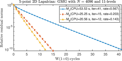
Figure 1: Example 1: comparison of multigrid convergence with different smoothers. Left: W(1+0)-cycle. Right: V(1+1)-cycle.

4.2 Example 2

In the second example we consider the following data

$$u=x\ln(x)y\ln(y),\ f=-x\ln(x)/y-y\ln(y)/x,\ g=0,$$

where $f$ has singularity near the boundary with $x=0$ or $y=0$. In Fig. 2, we compare the multigrid convergence performance of our considered three SPAI-type smoothers: $M_{J}$, $M_{5}$, and $M_{9}$, where the observed convergence rates are the same as those reported in Example 1. Again, we see V-cycle multigrid is more efficient than W-cycle multigrid. This example shows that the convergence rates of SPAI smoothers are not obviously influenced by the lower regularity of the given source term $f$.

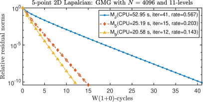
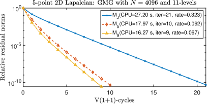
Figure 2: Example 2: comparison of multigrid convergence with different smoothers. Left: W(1+0)-cycle. Right: V(1+1)-cycle.

4.3 Example 3 [48]

In the third example, we consider the following 3D data

$$u=\sin(\pi x)\sin(\pi y)\sin(\pi z),\ f=3\pi^{2}\sin(\pi x)\sin(\pi y)\sin(\pi z),\ g=0.$$

In Fig. 3, we compare the multigrid convergence performance of the two SPAI-type smoothers: $M_{J}$ and $M_{7}$, where the observed convergence rates are compatible with the LFA predictions presented in Table 1. For both W and V cycles, $M_{7}$ takes about half of the CPU times by $M_{J}$, as predicted by Table 1. For all smoothers, we see that V-cycle is more efficient that W-cycle. We highlight that with $N=512$ the system has about 134 million unknowns, which takes about 200 seconds for $M_{7}$ with V-cycle.

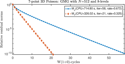
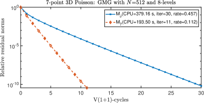
Figure 3: Example 3: comparison of multigrid convergence with different smoothers. Left: W(1+0)-cycle. Right: V(1+1)-cycle.

5 Conclusion

In this paper, we proposed and analyzed new 9-point and 7-point stencil based SPAI multigrid smoothers for solving 2D and 3D Laplacian linear systems respectively. The obtained optimal LFA smoothing factors are significantly smaller than that of the state-of-the-art SPAI smoothers in literature. The crucial optimal relaxation parameters are exactly derived through rigorous analysis. Numerical results with 2D and 3D examples validated our theoretical analysis and demonstrated the effectiveness of our proposed SPAI smoothers. It is interesting to extend such SPAI smoothers to general second-order elliptic PDEs with variable coefficients, see e.g. [37, 25] for the potential idea of preconditioning by inverting Laplacian with our proposed multigrid solvers. It is also possible to apply our proposed SPAI smoothers to elliptic optimal control problem [30] involving Laplacian. The MATLAB codes for implementing our proposed algorithms are publicly available online at the link: https://github.com/junliu2050/SPAI-MG-Laplacian.

Appendix A: a proof of Theorem 3.1

In this appendix, we provide a detail proof of Theorem 3.1 through several technical lemmas and propositions.

If $(\theta_{1},\theta_{2})\in T^{\rm{H}}=\left[-\frac{\pi}{2},\frac{3\pi}{2}\right)^{2}\setminus\left[-\frac{\pi}{2},\frac{\pi}{2}\right)^{2}$, then $(x_{1},x_{2}):=(\cos\theta_{1},\cos\theta_{2})\in X^{\rm{H}}:=[-1,1]^{2}\setminus(0,1]^{2}.$ Given $(a,b)\in\mathbb{R}^{2}$, we define

(0) $$f_{a,b}(x_{1},x_{2}):=[b+a(x_{1}+x_{2})+x_{1}x_{2}](2-x_{1}-x_{2}).$$

Then,

$$\mu_{\rm loc}=\max_{(x_{1},x_{2})\in X^{\rm{H}}}|1-\omega f_{a,b}(x_{1},x_{2})|.$$

By symmetry, we may assume without loss of generality that $x_{1}\leq x_{2}$. Hence,

(1) $$\mu_{\rm opt}=\min_{a,b,\omega}\max_{(x_{1},x_{2})\in X_{1}\cup X_{2}}|1-\omega f_{a,b}(x_{1},x_{2})|,$$

where

(2) $$X_{1}:= \{(x_{1},x_{2})\in\mathbb{R}^{2}:~{}-1\leq x_{1}\leq 0,~{}-x_{1}\leq x_{2}\leq 1\},$$

(3) $$X_{2}:= \{(x_{1},x_{2})\in\mathbb{R}^{2}:~{}-1\leq x_{1}\leq 0,~{}x_{1}\leq x_{2}\leq-x_{1}\}.$$

Since $X_{1}\cup X_{2}$ is compact, the extremes of $f_{a,b}$ on $X_{1}\cup X_{2}$ can be achieved. We denote

$$\chi_{a,b}:=\max_{(x_{1},x_{2})\in X_{1}\cup X_{2}}f_{a,b}(x_{1},x_{2}),~{}~{}m_{a,b}:=\min_{(x_{1},x_{2})\in X_{1}\cup X_{2}}f_{a,b}(x_{1},x_{2}).$$

Since $\widetilde{A}_{h}$ is positive, to guarantee the relaxation scheme convergent, we have to restrict $(a,b)$ in the following region

$$R:=\{(a,b)\in\mathbb{R}^{2}:m_{a,b}>0\}.$$

To find a SPAI smoother achieving the optimal smoothing factor, from (9), we need to solve the following minimization problem

(4) $$\mu_{\rm{opt}}=\min_{(a,b)\in R}J(a,b),$$

where

$$J(a,b)=(\chi_{a,b}-m_{a,b})/(\chi_{a,b}+m_{a,b}),$$

with the corresponding optimal choice of $\omega$ in the optimization problem (1) is

$$\omega_{\rm{opt}}=2/(\chi_{a,b}+m_{a,b}).$$

Moreover, by choosing $(x_{1},x_{2})$ to be $(-1,-1),(-1,0),(-1,1)$, and $(0,1)$, respectively, we obtain from the assumption $f_{a,b}(x_{1},x_{2})\geq m_{a,b}>0$ that

(5) $$b>1,~{}~{}b>|a|,~{}~{}b-2a+1>0,$$

provided $(a,b)\in R$. For $(x_{1},x_{2})\in X_{1}$, we have $x_{1}+x_{2}-1\leq x_{1}x_{2}\leq 0$ and hence,

$$u_{a,b}(x_{1}+x_{2})\leq f_{a,b}(x_{1},x_{2})\leq U_{a,b}(x_{1}+x_{2}),$$

where

$$u_{a,b}(t):=(b+at+t-1)(2-t),~{}~{}U_{a,b}(t):=(b+at)(2-t),$$

with $t=x_{1}+x_{2}\in[0,1]$. Since $b>1$ and $b>|a|$ by (5), we obtain

$$\max_{(x_{1},x_{2})\in X_{1}}f_{a,b}(x_{1},x_{2}) =\max_{t\in[0,1]}U_{a,b}(t)=\begin{cases}2b,&~{}b\geq 2a,\\ (b+2a)^{2}/(4a),&~{}b\leq 2a,\end{cases}$$

$$\min_{(x_{1},x_{2})\in X_{1}}f_{a,b}(x_{1},x_{2}) =\min_{t\in[0,1]}u_{a,b}(t)=\min\{b+a,2b-2\}.$$

For $(x_{1},x_{2})\in X_{2}$, we have $-(x_{1}+x_{2})-1\leq x_{1}x_{2}\leq(x_{1}+x_{2})^{2}/4,$ and hence, $v_{a,b}(-x_{1}-x_{2})\leq f_{a,b}(x_{1},x_{2})\leq V_{a,b}(-x_{1}-x_{2}),$ where

(6) $$v_{a,b}(t):=(b-at+t-1)(2+t),~{}~{}V_{a,b}(t):=(b-at+t^{2}/4)(2+t),$$

with $t=-x_{1}-x_{2}\in[0,2]$. Recall from (5) that $b>1$ and $b-2a+1>0$. It is easily seen that $v_{a,b}(t)$ is monotone for $t\in[0,2]$, and hence

$$\min_{(x_{1},x_{2})\in X_{2}}f_{a,b}(x_{1},x_{2})=\min_{t\in[0,2]}v_{a,b}(t)=\min\{4(b-2a+1),2b-2\}.$$

To find the maximum of $V_{a,b}(t)$ with $t\in[0,2]$, we shall investigate its derivative

$$V_{a,b}^{\prime}(t)=(-a+t/2)(2+t)+b-at+t^{2}/4=3t^{2}/4+(1-2a)t+b-2a.$$

If $(1-2a)^{2}<3(b-2a)$, then $V_{a,b}(t)$ is an increasing function for $t\in[0,2]$, and

$$\max_{(x_{1},x_{2})\in X_{2}}f_{a,b}(x_{1},x_{2})=V_{a,b}(1)=4(b-2a+1).$$

If $(1-2a)^{2}\geq 3(b-2a)$, then solving $V_{a,b}^{\prime}(t)=0$ gives two solutions

(7) $$t_{\pm}={2a-1\pm\sqrt{(1-2a)^{2}-3(b-2a)}\over 3/2}.$$

If $t_{-}\notin[0,2]$, then the maximum of $V_{a,b}(t)$ on $[0,2]$ is achieved at the end point, and

$$\max_{(x_{1},x_{2})\in X_{2}}f_{a,b}(x_{1},x_{2})=\max_{t\in[0,2]}V_{a,b}(t)=\max\{2b,4(b-2a+1)\}.$$

If $t_{-}\in[0,2]$, then the maximum of $V_{a,b}(t)$ on $[0,2]$ is achieved at $t_{-}$, and

$$\max_{(x_{1},x_{2})\in X_{2}}f_{a,b}(x_{1},x_{2})=V_{a,b}(t_{-})\geq V_{a,b}(0)=2b.$$

A combination of the above arguments gives the following lemma.

Lemma 0.1.

If $(a,b)\in R$, then $b>1,~{}~{}b>|a|,~{}~{}b-2a+1>0.$ Moreover,

$$m_{a,b}=\min\{b+a,2b-2,4(b-2a+1)\},$$

and

$$\chi_{a,b}=\begin{cases}\max\{\frac{(b+2a)^{2}}{4a},4(b-2a+1)\},&~{}b\leq 2a,\\ \max\{2b,4(b-2a+1)\},&~{}(1-2a)^{2}<3(b-2a),\\ \max\{2b,4(b-2a+1)\},&~{}(1-2a)^{2}\geq 3(b-2a)>0,~{}t_{-}\notin[0,2],\\ V_{a,b}(t_{-}),&~{}(1-2a)^{2}\geq 3(b-2a)>0,~{}t_{-}\in[0,2].\end{cases}$$

For convenience of discussion, we divide $R$ into four disjoint sub-regions:

$$R_{0} :=\{(a,b)\in R,~{}b\leq 2a\},$$

$$R_{1} :=\{(a,b)\in R,~{}(1-2a)^{2}<3(b-2a)\},$$

$$R_{2} :=\{(a,b)\in R,~{}(1-2a)^{2}\geq 3(b-2a)>0,~{}t_{-}\notin[0,2]\},$$

$$R_{3} :=\{(a,b)\in R,~{}(1-2a)^{2}\geq 3(b-2a)>0,~{}t_{-}\in[0,2]\}.$$

Recall that

(8) $$J(a,b)={\chi_{a,b}-m_{a,b}\over\chi_{a,b}+m_{a,b}}={1-r_{a,b}\over 1+r_{a,b}},~{}~{}r_{a,b}:={m_{a,b}\over\chi_{a,b}}\in(0,1].$$

We shall find lower bounds of $J(a,b)$ in the regions: $R_{0}$, $R_{1}\cup R_{2}$, and $R_{3}$, respectively.

Proposition 0.2.

If $(a,b)\in R_{0}$, then $J(a,b)\geq 1/5$.

Proof 0.3.

If $(a,b)\in R_{0}$, then $m_{a,b}=\min\{b+a,2b-2,4(b-2a+1)\},$ and $\chi_{a,b}=\max\{(b+2a)^{2}/(4a),4(b-2a+1)\}\geq(b+2a)^{2}/(4a)$. There are three cases:

1. $m_{a,b}=b+a$ and $\chi_{a,b}\geq(b+2a)^{2}/(4a)$. It can be shown that

   $$b\geq a+2,~{}b\geq 3a-4/3,~{}b\leq 2a,~{}2\leq a\leq 4/3,$$

   a contradiction. Thus, this case does not exist.

2. $m_{a,b}=2b-2$ and $\chi_{a,b}\geq(b+2a)^{2}/(4a)$. It can be shown that

   $$b\leq a+2,~{}b\geq 4a-3,~{}1<b\leq 2a,~{}1/2<a\leq 3/2,$$

   from which we further obtain

   $$r_{a,b}\leq{4a(2b-2)\over(b+2a)^{2}}\leq{8a(2a-1)\over(4a)^{2}}={2a-1\over 2a}\leq{2\over 3}.$$

3. $m_{a,b}=4(b-2a+1)$ and $\chi_{a,b}=(b+2a)^{2}/(4a)$. It can be shown that

   $$b\leq 3a-4/3,~{}2a-1<b\leq 4a-3,~{}b\leq 2a,~{}a>1.$$

   If $a\geq 3/2$, then we obtain from $b\leq 2a$ that

   $$r_{a,b}\leq{16a(b-2a+1)\over(b+2a)^{2}}\leq{16a\over(4a)^{2}}={1\over a}\leq{2\over 3}.$$

   If $a\leq 3/2$, then we obtain from $b\leq 4a-3$ that

   $$r_{a,b}\leq{16a(b-2a+1)\over(b+2a)^{2}}\leq{16a(2a-2)\over(6a-3)^{2}}\leq{24\over 6^{2}}={2\over 3}.$$

A combination of the above arguments yields $r_{a,b}\leq 2/3$ and hence $J(a,b)\geq 1/5$.

Proposition 0.4.

If $(a,b)\in R_{1}\cup R_{2}$, then $J(a,b)\geq 3/17$.

Proof 0.5.

If $(a,b)\in R_{1}\cup R_{2}$, then $m_{a,b}=\min\{b+a,2b-2,4(b-2a+1)\},$ and $\chi_{a,b}=\max\{2b,4(b-2a+1)\}$. There are six cases to be considered.

1. $m_{a,b}=b+a$ and $\chi_{a,b}=2b$. It can be shown that

   $$b\geq a+2,~{}b\geq 3a-4/3,~{}b\leq 4a-2,~{}a\geq 4/3,~{}b\geq 2a,$$

   from which we further obtain $(1-2a)^{2}\geq 3(b-2a)$ and $t_{-}\geq 0.$ Since $(a,b)\in R_{1}\cup R_{2}$, we have $t_{-}>2$, which implies $a>2$, $b>6a-5$, and

   $$r_{a,b}={1\over 2}+{a\over 2b}<{1\over 2}+{a\over 2(6a-5)}<{1\over 2}+{1\over 7}={9\over 14}.$$

2. $m_{a,b}=b+a$ and $\chi_{a,b}=4(b-2a+1)$. It can be shown that

   $$b\geq a+2,~{}b\geq 3a-4/3,~{}b\geq 4a-2.$$

   If $a\leq 1/3$, then $b+a\leq b-2a+2$, and

   $$r_{a,b}={b+a\over 4(b-2a+1)}\leq{1\over 4}.$$

   If $a\geq 4/3$, then we obtain from $b\geq 4a-2$ that

   $$r_{a,b}={b+a\over 4(b-2a+1)}\leq{5a-2\over 4(2a-1)}\leq{14/3\over 20/3}={7\over 10}.$$

   If $1/3\leq a\leq 4/3$, then we obtain from $b\geq a+2$ that

   $$r_{a,b}={b+a\over 4(b-2a+1)}\leq{2a+2\over 4(3-a)}\leq{14/3\over 20/3}={7\over 10}.$$

3. $m_{a,b}=2b-2$ and $\chi_{a,b}=2b$. It can be shown that

   $$b\leq a+2,~{}b\geq 4a-3,~{}1<b\leq 4a-2,~{}3/4<a\leq 5/3,$$

   from which we further obtain $(1-2a)^{2}\geq 3(b-2a)$ and $t_{-}\leq 2.$ Since $(a,b)\in R_{1}\cup R_{2}$, we have $t_{-}<0$, which implies $b<2a\leq 10/3$ and

   $$r_{a,b}=1-{1\over b}<{7\over 10}.$$

4. $m_{a,b}=2b-2$ and $\chi_{a,b}=4(b-2a+1)$. It can be shown that

   $$b\leq a+2,~{}b\geq 4a-3,~{}b\geq 4a-2,~{}a\leq 4/3.$$

   If $a\leq 1$, then $b-1\leq b-2a+1$ and $r_{a,b}={b-1\over 2(b-2a+1)}\leq{1\over 2}.$ If $a\geq 1$, then we obtain from $b\geq a+2$ and $a\leq 4/3$ that

   $$r_{a,b}={b-1\over 2(b-2a+1)}\leq{a+1\over 2(3-a)}\leq{7/3\over 10/3}={7\over 10}.$$

5. $m_{a,b}=4(b-2a+1)$ and $\chi_{a,b}=2b$. It can be shown that

   $$b\leq 3a-4/3,~{}b\leq 4a-3,~{}b\leq 4a-2,$$

   from which we further obtain $(1-2a)^{2}\geq 3(b-2a).$ It also follows from $b>1$ that $a>1$. Since $(a,b)\in R_{1}\cup R_{2}$, we have either $t_{-}<0$ or $t_{-}>2$. If $t_{-}>2$, then we have $a>2$ and $b>6a-5$, which contradicts $b\leq 4a-3$. Hence, we have $t_{-}<0$, and consequently, $b<2a$. If $a\geq 3/2$, then we obtain from $b<2a$ that

   $$r_{a,b}={2(b-2a+1)\over b}\leq{1\over a}\leq{2\over 3}.$$

   If $a\leq 3/2$, then we obtain from $b\leq 4a-3$ that

   $$r_{a,b}={2(b-2a+1)\over b}\leq{2(2a-2)\over 4a-3}\leq{2\over 3}.$$

6. $m_{a,b}=4(b-2a+1)$ and $\chi_{a,b}=4(b-2a+1)$. It can be shown that

   $$b\leq 3a-4/3,~{}b\leq 4a-3,~{}b\geq 4a-2,$$

   a contradiction. Hence, this case does not exist.

A combination of all cases gives $r_{a,b}\leq 7/10$ and $J(a,b)\geq 3/17$ for all $(a,b)\in R_{1}\cup R_{2}$.

It remains to find the lower bound of $J(a,b)$ in $R_{3}$. If $(a,b)\in R_{3}$, then $3b\leq 4a^{2}+2a+1$ and $0\leq t_{-}\leq 2$. From the quadrature formula of $t_{-}$ in (7), we obtain $a\geq(2+3t_{-})/4$, $b\geq 2a$ and

$$2a-4\leq\sqrt{4a^{2}+2a+1-3b}.$$

If $a\geq 2$, then $b\leq 6a-5$. It follows from $\chi_{a,b}\geq f_{a,b}(0,0)=2b$ and $m_{a,b}\leq f_{a,b}(0,1)=b+a$ that

$$r_{a,b}={m_{a,b}\over\chi_{a,b}}\leq{1\over 2}+{a\over 2b}\leq{1\over 2}+{a\over 2(6a-5)}<{1\over 2}+{1\over 7}={9\over 14}.$$

Now, we assume $a\leq 2$. Since $V_{a,b}^{\prime}(t_{-})=0$, we have $b=-3t_{-}^{2}/4+(2a-1)t_{-}+2a$. Recall that $m_{a,b}=\min\{b+a,2b-2,4(b-2a+1)\},$ and $\chi_{a,b}=V_{a,b}(t_{-})\geq\max\{2b,4(b-2a+1)\}$. We obtain

$$r_{a,b}={m_{a,b}\over\chi_{a,b}}={w(t_{-},a)\over W(t_{-},a)},$$

where $w(t_{-},a)=\min\{w_{1}(t_{-},a),w_{2}(t_{-},a),w_{3}(t_{-},a)\}$, and

$$w_{1}(t_{-},a) =b+a=-3t_{-}^{2}/4+(2a-1)t_{-}+3a=(2t_{-}+3)a-(3t_{-}^{2}/4+t_{-}),$$

$$w_{2}(t_{-},a) =2b-2=-3t_{-}^{2}/2+2(2a-1)t_{-}+4a-2$$

$$=(4t_{-}+4)a-(3t_{-}^{2}/2+2t_{-}+2),$$

$$w_{3}(t_{-},a) =4(b-2a+1)=-3t_{-}^{2}+4(2a-1)t_{-}+4=8t_{-}a-(3t_{-}^{2}+4t_{-}-4),$$

$$W(t_{-},a) =V_{a,b}(t_{-})=[-t_{-}^{2}/2+(a-1)t_{-}+2a](2+t_{-})$$

$$=[(t_{-}+2)a-(t_{-}^{2}/2+t_{-})](t_{-}+2).$$

Replacing $t_{-}$ with $t$ in the above formulas, we obtain the bi-variate polynomials $w_{1}(t,a),~{}w_{2}(t,a),~{}w_{3}(t,a)$, and $W(t,a)$. Denote

(9) $$r^{*}:=\max_{(t,a)\in S}{w(t,a)\over W(t,a)},$$

where

$$S:=\{(t,a)\in\mathbb{R}^{2}:0\leq t\leq 2,~{}(3t+2)/4\leq a\leq 2\}.$$

The above arguments can be summarized in the following lemma.

Lemma 0.6.

For any $(a,b)\in R_{3}$ with $a\geq 2$, we have $r_{a,b}\leq 9/14$. For any $(a,b)\in R_{3}$ with $a\leq 2$, we have $r_{a,b}\leq r^{*}$.

Next, we will estimate $r^{*}$ in a sequence of lemmas.

Lemma 0.7.

Fix $t\in[0,2]$. The functions $w_{1}(t,a),w_{2}(t,a),w_{3}(t,a),W(t,a)$ are linear, monotonically increasing, and positive for $(3t+2)/4<a\leq 2$. The functions $w_{1}(t,a),w_{3}(t,a),W(t,a)$ are positive and $w_{2}(t,a)\geq 0$ at $a=(3t+2)/4$. Moreover,

1. If $t\in(0,2)$, then the rational functions $w_{1}(t,a)/W(t,a)$, $w_{2}(t,a)/W(t,a)$, and $w_{3}(t,a)/W(t,a)$, respectively, are monotonically decreasing, increasing, and decreasing for $a\in[(3t+2)/4,2]$.

2. If $t=0$, then $w_{1}(t,a)/W(t,a)$ is a constant function, $w_{2}(t,a)/W(t,a)$ is an increasing function, and $w_{3}(t,a)/W(t,a)$ is a decreasing function for $a\in[(3t+2)/4,2]$.

3. If $t=2$, then the interval $[(3t+2)/4,2]$ shrinks to a point $2$.

Proof 0.8.

It is obvious that the linear functions $w_{1}(t,a),w_{2}(t,a),w_{3}(t,a),W(t,a)$ have positive leading coefficients and are monotonically increasing. We verify that

$$w_{1}(t,(3t+2)/4) =(2t+3)(3t+2)/4-(3t^{2}/4+t)=3t^{2}/4+9t/4+3/2>0,$$

$$w_{2}(t,(3t+2)/4) =(4t+4)(3t+2)/4-(3t^{2}/2+2t+2)=3t^{2}/2+3t\geq 0,$$

$$w_{3}(t,(3t+2)/4) =8t(3t+2)/4-(3t^{2}+4t-4)=3t^{2}+4>0,$$

$$W(t,(3t+2)/4) =[(t+2)(3t+2)/4-(t^{2}/2+t)](t+2)=(t^{2}/4+t+1)(t+2)>0.$$

This proves that $w_{1}(t,a),w_{3}(t,a),W(t,a)$ are positive at $a=(3t+2)/4$, and $w_{2}(t,a)\geq 0$ at $a=(3t+2)/4$. Consequently, all functions $w_{1}(t,a),w_{2}(t,a),w_{3}(t,a),W(t,a)$ are positive for $(3t+2)/4<a\leq 2$.

For any $k_{1}>0$ and $k_{2}>0$, the Möbius transform [2]

$${k_{1}x-b_{1}\over k_{2}x-b_{2}}={k_{1}\over k_{2}}+{k_{1}b_{2}-k_{2}b_{1}\over k_{2}(k_{2}x-b_{2})}$$

is an increasing (resp. decreasing) function for $x>b_{2}/k_{2}$ if $k_{1}b_{2}-k_{2}b_{1}$ is negative (resp. positive). Given $t\in(0,2)$, it then follows from

$$(2t+3)(t^{2}/2+t)-(t+2)(3t^{2}/4+t) =t^{3}/4+t^{2}+t>0,$$

$$(4t+4)(\frac{1}{2}t^{2}+t)-(t+2)(\frac{3}{2}t^{2}+2t+2) =\frac{1}{2}t^{3}+t^{2}-2t-4=\frac{1}{2}(t+2)^{2}(t-2)<0,$$

$$8t(t^{2}/2+t)-(t+2)(3t^{2}+4t-4) =t^{3}-2t^{2}-4t+8=(t-2)^{2}(t+2)>0$$

that the rational functions $w_{1}(t,a)/W(t,a)$, $w_{2}(t,a)/W(t,a)$, and $w_{3}(t,a)/W(t,a)$, respectively, are monotonically decreasing, increasing, and decreasing for $a\in[(3t+2)/4,2]$. The proof for the cases $t=0$ and $t=2$ are trivial.

Lemma 0.9.

If $t\in[1,2]$, then $w(t,a)=w_{1}(t,a)$ and $w(t,a)/W(t,a)\leq 2/3$ for all $a\in[(3t+2)/4,2]$.

Proof 0.10.

For any $a\in[(3t+2)/4,2]$, since

$$w_{2}(t,a)-w_{1}(t,a) =(2t+1)a-(3t^{2}/4+t+2)$$

$$\geq(2t+1)(3t+2)/4-(3t^{2}/4+t+2)=3(t-1)(t+2)/4\geq 0,$$

and

$$w_{3}(t,a)-w_{1}(t,a) =(6t-3)a-(9t^{2}/4+3t-4)$$

$$\geq(6t-3)(3t+2)/4-(9t^{2}/4+3t-4)=9t^{2}/4-9t/4+5/2>0,$$

we have $w(t,a)=\min\{w_{1}(t,a),w_{2}(t,a),w_{3}(t,a)\}=w_{1}(t,a)$. Consequently,

$${w(t,a)\over W(t,a)}\leq{w_{1}(t,(3t+2)/4)\over W(t,(3t+2)/4)}={3(t+1)\over(t+2)^{2}}\leq{2\over 3}.$$

This completes the proof.

Lemma 0.11.

If $t\in[1/2,1]$, then $w_{1}(t,a)<w_{3}(t,a)$ and $w(t,a)/W(t,a)\leq 24/35$ for all $a\in[(3t+2)/4,2]$.

Proof 0.12.

It is easily seen that

$$w_{3}(t,a)-w_{1}(t,a) =(6t-3)a-(9t^{2}/4+3t-4)$$

$$\geq(6t-3)(3t+2)/4-(9t^{2}/4+3t-4)=9t^{2}/4-9t/4+5/2>0.$$

We also note that

$$w_{2}(t,(3t+2)/4)-w_{1}(t,(3t+2)/4) =3(t-1)(t+2)/2\leq 0.$$

If $a\geq(3t^{2}/4+t+2)/(2t+1)$, then

$$w_{2}(t,a)-w_{1}(t,a)=(2t+1)a-(3t^{2}/4+t+2)\geq 0,$$

which implies $w(t,a)=w_{1}(t,a)$, and hence

$${w(t,a)\over W(t,a)} \leq{w_{1}(t,(3t^{2}/4+t+2)/(2t+1))\over W(t,(3t^{2}/4+t+2)/(2t+1))}={6(t+2)\over-t^{3}+12t+16}\leq{24\over 35}.$$

If $a\leq(3t^{2}/4+t+2)/(2t+1)$, then

$$w_{2}(t,a)-w_{1}(t,a)=(2t+1)a-(3t^{2}/4+t+2)\leq 0,$$

which implies $w(t,a)=w_{2}(t,a)$ and

$${w(t,a)\over W(t,a)} \leq{w_{2}(t,(3t^{2}/4+t+2)/(2t+1))\over W(t,(3t^{2}/4+t+2)/(2t+1))}={6(t+2)\over-t^{3}+12t+16}\leq{24\over 35}.$$

The proof is completed.

Lemma 0.13.

If $t\in[0,1/2]$, then $w(t,a)/W(t,a)\leq(68-5\sqrt{10})/72$ for all $a\in[(3t+2)/4,2]$.

Proof 0.14.

We have to consider three cases.

1. $w(t,a)=w_{1}(t,a)$. It follows from

   $$0\leq w_{2}(t,a)-w_{1}(t,a)=(2t+1)a-(3t^{2}/4+t+2),$$

   and

   $$0\geq w_{1}(t,a)-w_{3}(t,a)=(3-6t)a-(4-3t-9t^{2}/4)$$

   that

   $${3t^{2}/4+t+2\over 2t+1}\leq a\leq{4-3t-9t^{2}/4\over 3-6t},$$

   which together with $t\in[0,2]$ gives $t\geq t_{0}:={14-4\sqrt{10}\over 9}.$ Consequently,

   $${w(t,a)\over W(t,a)} \leq{w_{1}(t,(3t^{2}/4+t+2)/(2t+1))\over W(t,(3t^{2}/4+t+2)/(2t+1))}={6(t+2)\over-t^{3}+12t+16}\leq{68-5\sqrt{10}\over 72}.$$

2. $w(t,a)=w_{2}(t,a)$. It follows from

   $$0\geq w_{2}(t,a)-w_{1}(t,a)=(2t+1)a-(3t^{2}/4+t+2),$$

   and

   $$0\geq w_{2}(t,a)-w_{3}(t,a)=(4-4t)a-(6-2t-3t^{2}/2)$$

   that

   $$a\leq\min\{{3t^{2}/4+t+2\over 2t+1},{6-2t-3t^{2}/2\over 4-4t}\}.$$

   If

   $${3t^{2}/4+t+2\over 2t+1}\leq{6-2t-3t^{2}/2\over 4-4t},$$

   then $t\geq t_{0}:={14-4\sqrt{10}\over 9},$ and

   $${w(t,a)\over W(t,a)} \leq{w_{2}(t,(3t^{2}/4+t+2)/(2t+1))\over W(t,(3t^{2}/4+t+2)/(2t+1))}={6(t+2)\over-t^{3}+12t+16}\leq{68-5\sqrt{10}\over 72}.$$

   If

   $${3t^{2}/4+t+2\over 2t+1}\geq{6-2t-3t^{2}/2\over 4-4t},$$

   then $t\leq t_{0}:={14-4\sqrt{10}\over 9},$ and

   $${w(t,a)\over W(t,a)} \leq{w_{2}(t,(6-2t-3t^{2}/2)/(4-4t))\over W(t,(6-2t-3t^{2}/2)/(4-4t))}$$

   $$={8(2+3t)\over(12+4t-t^{2})(2+t)}\leq{68-5\sqrt{10}\over 72}.$$

3. $w(t,a)=w_{3}(t,a)$. It follows from

   $$0\leq w_{1}(t,a)-w_{3}(t,a)=(3-6t)a-(4-3t-9t^{2}/4)$$

   and

   $$0\leq w_{2}(t,a)-w_{3}(t,a)=(4-4t)a-(6-2t-3t^{2}/2)$$

   that

   $$a\geq\max\{{4-3t-9t^{2}/4\over 3-6t},{6-2t-3t^{2}/2\over 4-4t}\}.$$

   If

   $${4-3t-9t^{2}/4\over 3-6t}\geq{6-2t-3t^{2}/2\over 4-4t},$$

   then $t\geq t_{0}:={14-4\sqrt{10}\over 9},$ and

   $${w(t,a)\over W(t,a)} \leq{w_{3}(t,(4-3t-9t^{2}/4)/(3-6t))\over W(t,(4-3t-9t^{2}/4)/(3-6t))}$$

   $$={4(-9t^{2}-4t+12)\over(3t^{2}-18t+16)(t+2)^{2}}\leq{68-5\sqrt{10}\over 72}.$$

   If

   $${4-3t-9t^{2}/4\over 3-6t}\leq{6-2t-3t^{2}/2\over 4-4t},$$

   then $t\leq t_{0}:={14-4\sqrt{10}\over 9},$ and

   $${w(t,a)\over W(t,a)} \leq{w_{3}(t,(6-2t-3t^{2}/2)/(4-4t))\over W(t,(6-2t-3t^{2}/2)/(4-4t))}$$

   $$={8(2+3t)\over(12+4t-t^{2})(2+t)}\leq{68-5\sqrt{10}\over 72}.$$

This completes the proof.

A combination of the above lemmas gives $r_{a,b}\leq r^{*}\leq(68-5\sqrt{10})/72$ for $(a,b)\in R_{3}$. Since $J(a,b)=(1-r_{a,b})/(1+r_{a,b})$, we have the following result.

Proposition 0.15.

If $(a,b)\in R_{3}$, then $J(a,b)\geq(9+8\sqrt{10})/215$.

Proof 0.16 (Proof of Theorem 3.1).

It follows from Propositions 0.2, 0.4, and 0.15 that

$$J(a,b)\geq(9+8\sqrt{10})/215$$

for all $(a,b)\in R=R_{0}\cup R_{1}\cup R_{2}\cup R_{3}$. On the other hand, by choosing $(a,b)=(5/3,11/3)\in R_{3}$, we obtain from a simple calculation that

$$J(5/3,11/3)=(9+8\sqrt{10})/215$$

with $m_{5/3,11/3}=16/3$ and $\chi_{5/3,11/3}=(4352+320\sqrt{10})/729$. Hence, we have

$$\mu_{\rm{opt}}=\min_{(a,b)\in R}J(a,b)={9+8\sqrt{10}\over 215},$$

and the corresponding optimal value of $\omega$ is calculated as

$$\omega_{\rm{opt}}={2\over m_{5/3,11/3}+\chi_{5/3,11/3}}={309-12\sqrt{10}\over 1720},$$

which completes the proof of Theorem 3.1.

References

- [1] M. Adams, M. Brezina, J. Hu, and R. Tuminaro, Parallel multigrid smoothing: polynomial versus Gauss–Seidel, Journal of Computational Physics, 188 (2003), pp. 593–610.
- [2] D. N. Arnold and J. P. Rogness, Möbius transformations revealed, Notices of the American Mathematical Society, 55 (2008), pp. 1226–1231.
- [3] A. H. Baker, R. D. Falgout, T. V. Kolev, and U. M. Yang, Multigrid smoothers for ultraparallel computing, SIAM Journal on Scientific Computing, 33 (2011), pp. 2864–2887.
- [4] M. Benzi, C. D. Meyer, and M. Tûma, A sparse approximate inverse preconditioner for the conjugate gradient method, SIAM Journal on Scientific Computing, 17 (1996), pp. 1135–1149.
- [5] M. Benzi and M. Tuma, A sparse approximate inverse preconditioner for nonsymmetric linear systems, SIAM Journal on Scientific Computing, 19 (1998), pp. 968–994.
- [6] M. Benzi and M. Tûma, A comparative study of sparse approximate inverse preconditioners, Applied Numerical Mathematics, 30 (1999), pp. 305–340.
- [7] D. Bertaccini and F. Durastante, Iterative methods and preconditioning for large and sparse linear systems with applications, Chapman and Hall/CRC, 2018.
- [8] D. Bertaccini and S. Filippone, Sparse approximate inverse preconditioners on high performance GPU platforms, Computers & Mathematics with Applications, 71 (2016), pp. 693–711.
- [9] P. Birken, Designing optimal smoothers for multigrid methods for unsteady flow problems, in 20th AIAA Computational Fluid Dynamics Conference, 2011, p. 3233.
- [10] M. Bolten, T. K. Huckle, and C. D. Kravvaritis, Sparse matrix approximations for multigrid methods, Linear Algebra and its Applications, 502 (2016), pp. 58–76.
- [11] D. Braess, The contraction number of a multigrid method for solving the Poisson equation, Numerische Mathematik, 37 (1981), pp. 387–404.
- [12] D. Braess, The convergence rate of a multigrid method with Gauss-Seidel relaxation for the Poisson equation, in Multigrid methods, Springer, 1982, pp. 368–386.
- [13] D. Braess, The convergence rate of a multigrid method with Gauss-Seidel relaxation for the Poisson equation, Mathematics of computation, 42 (1984), pp. 505–519.
- [14] H. Brandén, Grid independent convergence using multilevel circulant preconditioning: Poisson’s equation, BIT Numerical Mathematics, 62 (2022), pp. 409–429.
- [15] A. Brandt, Multi-level adaptive solutions to boundary-value problems, Mathematics of Computation, 31 (1977), pp. 333–390.
- [16] J. Brannick, X. Hu, C. Rodrigo, and L. Zikatanov, Local Fourier analysis of multigrid methods with polynomial smoothers and aggressive coarsening, Numerical Mathematics: Theory, Methods and Applications, 8 (2015), pp. 1–21.
- [17] W. L. Briggs, V. E. Henson, and S. F. McCormick, A multigrid tutorial, SIAM, Philadelphia, PA, 2000.
- [18] O. Bröker, Sparse approximate inverse smoothers for geometric and algebraic multigrid, Applied Numerical Mathematics, 41 (2002), pp. 61–80.
- [19] O. Bröker, M. J. Grote, C. Mayer, and A. Reusken, Robust parallel smoothing for multigrid via sparse approximate inverses, SIAM Journal on Scientific Computing, 23 (2001), pp. 1396–1417.
- [20] J. Brown, Y. He, S. MacLachlan, M. Menickelly, and S. M. Wild, Tuning multigrid methods with robust optimization and local fourier analysis, SIAM Journal on Scientific Computing, 43 (2021), pp. A109–A138.
- [21] J. Cosgrove, J. Diaz, and A. Griewank, Approximate inverse preconditionings for sparse linear systems, International Journal of Computer Mathematics, 44 (1992), pp. 91–110.
- [22] Á. P. de la Riva, C. Rodrigo, and F. J. Gaspar, A two-level method for isogeometric discretizations based on multiplicative Schwarz iterations, Computers & Mathematics with Applications, 100 (2021), pp. 41–50.
- [23] F. J. Gaspar, J. L. Gracia, and F. J. Lisbona, Fourier analysis for multigrid methods on triangular grids, SIAM Journal on Scientific Computing, 31 (2009), pp. 2081–2102.
- [24] F. J. Gaspar, J. L. Gracia, F. J. Lisbona, and C. Rodrigo, On geometric multigrid methods for triangular grids using three-coarsening strategy, Applied Numerical Mathematics, 59 (2009), pp. 1693–1708.
- [25] T. Gergelits, K.-A. Mardal, B. F. Nielsen, and Z. Strakos, Laplacian preconditioning of elliptic PDEs: Localization of the eigenvalues of the discretized operator, SIAM Journal on Numerical Analysis, 57 (2019), pp. 1369–1394.
- [26] N. I. Gould and J. A. Scott, Sparse approximate-inverse preconditioners using norm-minimization techniques, SIAM Journal on Scientific Computing, 19 (1998), pp. 605–625.
- [27] C. Greif and Y. He, A closed-form multigrid smoothing factor for an additive Vanka-type smoother applied to the Poisson equation, arXiv preprint arXiv:2111.03190, (2021).
- [28] M. J. Grote and T. Huckle, Parallel preconditioning with sparse approximate inverses, SIAM Journal on Scientific Computing, 18 (1997), pp. 838–853.
- [29] T. Guillet and R. Teyssier, A simple multigrid scheme for solving the Poisson equation with arbitrary domain boundaries, Journal of Computational Physics, 230 (2011), pp. 4756–4771.
- [30] Y. He and J. Liu, Smoothing analysis of two robust multigrid methods for elliptic optimal control problems, arXiv preprint arXiv:2203.13066, (2022).
- [31] Y. He and S. MacLachlan, Two-level Fourier analysis of multigrid for higher-order finite-element discretizations of the Laplacian, Numerical Linear Algebra with Applications, 27 (2020), p. e2285.
- [32] L. R. Hocking and C. Greif, Closed-form multigrid smoothing factors for lexicographic Gauss-Seidel, IMA Journal of Numerical Analysis, 32 (2011), pp. 795–812.
- [33] W. H. Holter, A vectorized multigrid solver for the three-dimensional Poisson equation, Applied mathematics and computation, 19 (1986), pp. 127–144.
- [34] R. Huang, R. Li, and Y. Xi, Learning optimal multigrid smoothers via neural networks, arXiv preprint arXiv:2102.12071, (2021).
- [35] J. Kraus, P. Vassilevski, and L. Zikatanov, Polynomial of best uniform approximation to and smoothing in two-level methods, Computational Methods in Applied Mathematics, 12 (2012), pp. 448–468.
- [36] J. Lottes, Optimal polynomial smoothers for multigrid V-cycles, arXiv preprint arXiv:2202.08830, (2022).
- [37] B. F. Nielsen, A. Tveito, and W. Hackbusch, Preconditioning by inverting the Laplacian: an analysis of the eigenvalues, IMA Journal of Numerical Analysis, 29 (2009), pp. 24–42.
- [38] Y. Notay and A. Napov, A massively parallel solver for discrete Poisson-like problems, Journal of Computational Physics, 281 (2015), pp. 237–250.
- [39] K. Pan, D. He, and H. Hu, An extrapolation cascadic multigrid method combined with a fourth-order compact scheme for 3D poisson equation, Journal of Scientific Computing, 70 (2017), pp. 1180–1203.
- [40] C. Rodrigo, On the validity of the local Fourier analysis, Journal of Computational Mathematics, 37 (2019), pp. 340–348.
- [41] Y. Saad, Iterative Methods for Sparse Linear Systems: Second Edition, SIAM, Philadelphia, PA, 2003.
- [42] W.-P. Tang, Toward an effective sparse approximate inverse preconditioner, SIAM Journal on Matrix Analysis and Applications, 20 (1999), pp. 970–986.
- [43] W.-P. Tang and W. L. Wan, Sparse approximate inverse smoother for multigrid, SIAM Journal on Matrix Analysis and Applications, 21 (2000), pp. 1236–1252.
- [44] U. Trottenberg, C. W. Oosterlee, and A. Schuller, Multigrid, Academic press, 2000.
- [45] R. Wienands and W. Joppich, Practical Fourier analysis for multigrid methods, CRC press, 2004.
- [46] X. Yang and R. Mittal, Efficient relaxed-Jacobi smoothers for multigrid on parallel computers, Journal of Computational Physics, 332 (2017), pp. 135–142.
- [47] J. Zhang, Acceleration of five-point red-black Gauss-Seidel in multigrid for Poisson equation, Applied Mathematics and Computation, 80 (1996), pp. 73–93.
- [48] J. Zhang, Fast and high accuracy multigrid solution of the three dimensional Poisson equation, Journal of Computational Physics, 143 (1998), pp. 449–461.