Opportunistic Routing aided Cooperative Communication MRC Network with Energy-Harvesting Nodes

Abstract

In this research, we present a cooperative communication network based on two energy-harvesting (EH) decode-and-forward (DF) relays that contain the harvest-store-use (HSU) architecture and may harvest energy from the surrounding environment by utilizing energy buffers. To improve the performance of this network, an opportunistic Routing (OR) algorithm is presented that takes into account channel status information, relay position, and energy buffer status, as well as using the maximal ratio combining (MRC) at the destination to combine the signals received from the source and relays. The theoretical expressions for limiting distribution of energy stored in infinite-size buffers are derived from the discrete-time continuous-state space Markov chain model (DCSMC). In addition, the theoretical expressions for outage probability, throughput, and per-packet timeslot cost in the network are obtained utilizing both the limiting distributions of energy buffers and the probabilities of transmitter candidates set. Through numerous simulation results, it is demonstrated that simulation results match with corresponding theoretical results.

I Introduction

In recent years, due to the emphasis on green communications, there has been a great deal of interest in EH technique, which can harvest energy from the surrounding ambient source such as radio frequency energy, light energy, thermal energy, etc[1]. In addition to the advantages of energy saving, EH can also extend battery lifetime compared to the source charging the battery, which is helpful in the complicated case of replacing the battery[2]. For these reasons, numerous articles emphasize the combination of EH and communications.

In [3], a relay selection approach for the EH wireless body area network that takes into account both channel state information (CSI) and the energy condition of the relay buffer is proposed. For the sake of obtaining a tradeoff between the transmission energy and decoding energy, the power splitting protocol is employed at the EH relay of the EH-based cooperative communication network in [4] and [5]. In these papers, the harvest-use (HU) architecture is employed to manage energy, meaning that the node will instantly use the gathered energy.

On the other hand, the harvest-store-use (HSU) architecture, which is widely explored as an efficient technique of energy harvesting from the environment, is comprised of three energy management steps: energy harvesting, energy storage, and energy use. In [6], a simple communication system with EH using HSU architecture is proposed, assuming that the EH node harvests energy from a radio frequency signal broadcast by an access point in the downlink and uses the stored energy to transmit data in the uplink. Unlike [6], which only investigated the on-off policy, both the best-effort policy and the on-off policy are analyzed in [7]. Both [6] and [7] derived the limiting distribution of stored energy in the energy buffer at the EH node by using the theory of discrete-time continuous-state Markov chains. The difference between the on-off policy and the best-effort policy is whether set target energy to transmit information or not. In the on-off policy, only when target M units of energy are available in the energy buffer, the EH node can transmit information to the destination at the cost of M units of energy. In the best-effort policy, no matter how much energy is in the energy buffer, the EH node uses all energy to transmit information to the destination. To maximize the end-to-end system throughput under data and energy storage constraints, the online and offline optimization algorithms for joint relay selection and power control have been discussed in [8].

In the aforementioned papers, all EH nodes harvest energy from RF signals received from the downlink, which is not efficient when the path loss in practical communication links is high. And they only consider the relay link without a direct link. The self-sustaining node (SSN), which harvests energy from the ambiance, is regarded as a solution to the high path loss link in the EH network. Self-sustaining node and direct link are covered in [9], where the limiting distributions of energy for both the incremental on-off policy and the incremental best-effort policy are derived by using a discrete-time continuous-state space Markov chain. In addition, the expressions for outage probability and throughput are obtained. In this process, the maximal ratio combining technique is used to improve the performance of the network. In all of the papers mentioned above, each source node in the cooperative relay network is powered by the power source. For the sake of further energy saving, the source node is equipped with the EH technique in [10]. A decoded-and-forward energy-harvesting system with multiple relays in the presence of transmitting hardware impairments is proposed in [11]. The system has two transmitting policies. For policy-1, the selection of the best relay that assists the source-to-destination communication is based on the first-hop channel-state-information. For policy-2, the selection of the best relay is based on the second-hop CSI.

All relay networks mentioned above are primarily founded on wireless two-hop relay networks with a single relay or multiple relays with the same priority. However, actually, the practical wireless cooperative network like a wireless sensor network[12] or an Internet of Things (IoT) network[13] is the wireless multi-hop network. Opportunistic routing as a solution to improve the performance of the wireless multi-top network has been widely studied[14]. An energy-efficient OR, which exploits cross-layer information exchange and Energy-consumption-based Objective Functions, is proposed in [15] and [16] where it has been clarified that OR outperforms the traditional routing with the specific preselected route in terms of system performance. And in [17], with using OR algorithm, a cooperative communication network based on two energy-harvesting decode-and-forward relays is proposed.

TABLE I: Comparsion of references

Reference	EH buffer architecture	SSN	OR	MRC
[3],[4],[5]	HU	N	N	N
[6],[7],[8]	HSU	N	N	N
[9],[10]	HSU	Y	N	Y
[11]	HSU	Y	N	N
[14]–[16]	No EH	N	Y	N
[17]	HSU	Y	Y	N
[18]	No EH	N	N	Y
Our work	HSU	Y	Y	Y

According to the above researches, maximal-ratio combining as a well-studied technique[18], which is helpful to improve performance in communication networks, is worth being combined with EH. This article is targeted at proposing and designing an analytical framework for the study of OR-aided cooperative communication networks with EH nodes and using MRC in our system. Table I shows the comparison between our work and the above references, where N indicates that the technology is not employed in the studied system, and Y indicates that the technology is employed in the studied system. In addition, we model energy buffers using discrete-time continuous-state space Markov chains. The contributions of this work are as follows:

1. A cooperative network consisting of two EH DF relay nodes and employing the MRC and OR algorithms is proposed.

2. The expressions for the limiting distributions of energy stored in buffers are obtained with the help of the DCSMC model and the state-transition-matrix-based (STM) theoretical solutions of the probability of transmitter candidates set. The limiting distributions of energy are the base of further analysis.

3. The closed-form expressions of outage probability and throughput are derived.

4. Through numerous simulation results, it is demonstrated that simulation results match with corresponding theoretical results.

The remaining paper is developed as follows: Section II interprets the system model and OR protocol. In section III, the limiting PDFs of the energy stored in the buffers R1 and R2 are presented. In section IV, the expressions for outage probability and throughput are determined. In Section V, simulation performance results are displayed. Section VI is where the conclusion is provided.

$Notations:$

TABLE II: Notations table

Notation	Meaning
$A\sim\mathcal{CN}(0,\theta)$	the random variable $A$ follows the complex Gaussian distribution with mean 0 and variance $\theta$
$|B|$	the absolute value of $B$
$\mathbb{E}[\cdot]$	the expectation operator
$C_{1}\cup C_{2}$	the union of the condition $C_{1}$ and the condition $C_{2}$
$C_{1}\cap C_{2}$	the intersection of the condition $C_{1}$ and the condition $C_{2}$
$W(\cdot)$	the Lambert W function
Boldface capital T	matrices or vectors
$\overline{\mathbb{C}}$	the comlementary event of $\mathbb{C}$
$*$	multiplication
$|$	conditional probability. For example, case A,B—C means event A and B occur under the condition of C.
conv$(A,B)$	discrete convolution $y(j)=\mathrm{conv}(A,B)=\sum_{i=-\infty}^{+\infty}A(i)B(j-i)$

In TABLE II, all notations are showed.

$Abbreviation:$

TABLE III: Abbreviations table

Abbreviation	Meaning
EH	energy harvesting
DF	decode and forward
HSU	harvest-store-use
OR	opportunistic routing
MRC	maximal ratio combing
DCSMC	discrete-time continuous-state space Markov chain
CSI	channel state information
HU	harvest-use
SSN	self-sustaining node
PEB	primary energy buffer
SEB	secondary energy buffer
ACK	positive acknowledgement
NACK	negative acknowledgement
TC	transmitter candidate

In TABLE III, all abbreviations are showed.

II System Model and OR Protocol

II-A System Model

As shown in Fig. 1, the network proposed in this paper is composed of a source node S, two DF relay nodes R1 and R2, and a destination node D. All nodes are assumed as half-duplex nodes. Only the source and destination nodes are powered by the power supply, while relay nodes are equipped with energy buffers using HSU architectures to harvest ambient energy. In each time slot, only one node is activated and can transmit signals by broadcast way, while others are silent or receive the signals. Quasi-static Rayleigh fading is assumed between all nodes. Let $d_{ab}$ denote the distance between nodes with a and b. Hence, denoted by $h_{SD}(i)\sim\mathcal{CN}(0,d_{SD}^{\alpha})$, $h_{SR1}(i)\sim\mathcal{CN}(0,d_{SR1}^{\alpha})$, $h_{SR2}(i)\sim\mathcal{CN}(0,d_{SR2}^{\alpha})$, $h_{R1R2}(i)\sim\mathcal{CN}(0,d_{R1R2}^{\alpha})$, $h_{R1D}(i)\sim\mathcal{CN}(0,d_{R1D}^{\alpha})$ and $h_{R2D}(i)\sim\mathcal{CN}(0,d_{R2D}^{\alpha})$ the channel coefficients within the $i$-th time slot between S and D, S and R1, S and R2, R1 and R2, R1 and D, and R2 and D respectively, where the term $\alpha$ represents the path-loss exponent.

The HSU architectures equipped by the relay nodes mainly have two energy buffers respectively, which are an infinite-size primary energy buffer (PEB) and an infinite-size secondary energy buffer (SEB), for the reason that storage devices are disabled to charge and discharge at the same time [19] [20]. The energy harvested from ambiance is stored in SEB first. Then, in order to make the energy buffer equipped by relay nodes R1 and R2 charge and discharge simultaneously, SEB transfers the energy to the PEB at the end of each timeslot. Finally, the energy in PEB is used to power the node to transmit signals. Due to the fact that the energy harvesting power is far smaller than the actual energy buffer capacity, the capacity of the energy buffer is considered to be infinite size in the theoretical analysis. In [20], it is indicated that there is no energy loss during charging between SEB and PEB or discharging between PEB and the node transmitter. The signals received from S, R1, and R2 are combined using MRC at D.

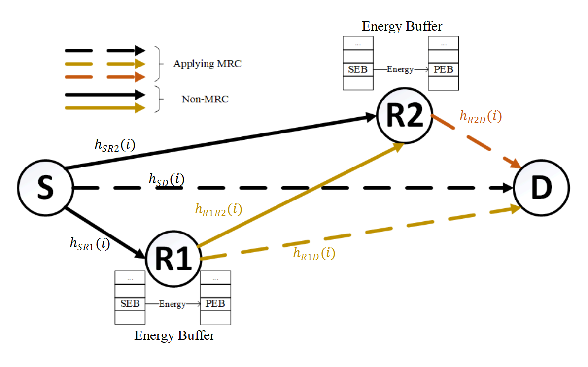
Figure 1: System model

The source S broadcasts unit-energy symbols $x_{S}(i)$ to relay R1, relay R2, and destination D at rate $R_{0}$ with the constant power $P_{S}$. The received signals $y_{SR1}(i)$, $y_{SR2}(i)$ and $y_{SD}(i)$ at relay R1, relay R2 and destination D in the $i$-th time slot are given by

$$y_{SR1}(i)=\sqrt{P_{S}}h_{SR1}(i)x_{S}(i)+n_{SR1}(i),$$ (1)

$$y_{SR2}(i)=\sqrt{P_{S}}h_{SR2}(i)x_{S}(i)+n_{SR2}(i),$$ (2)

$$y_{SD}(i)=\sqrt{P_{S}}h_{SD}(i)x_{S}(i)+n_{SD}(i),$$ (3)

where, $n_{SR1}(i)$, $n_{SR2}(i)$ and $n_{SD}(i)\sim\mathcal{CN}(0,N_{0})$ represent the received additive white Gaussian noise (AWGN) at R1, R2 and D, respectively. Thus, the received signal-to-noise ratios (SNRs) $\gamma_{SR1}(i)$, $\gamma_{SR2}(i)$ and $\gamma_{SD}(i)$ at R1, R2 and D in the $i$-th time slot would be given as follows

$$\begin{split}&\gamma_{SR1}(i)=\frac{P_{S}|h_{SR1}(i)|^{2}}{N_{0}},\quad\gamma_{SR2}(i)=\frac{P_{S}|h_{SR2}(i)|^{2}}{N_{0}}\\ &\mbox{ and }\quad\gamma_{SD}(i)=\frac{P_{S}|h_{SD}(i)|^{2}}{N_{0}}.\end{split}$$ (4)

As a DF relay, the relay R1 decodes the received signals, re-encodes them into unit-energy symbols $x_{R1}(i)$, and then broadcasts $x_{R1}(i)$ to relay R2 and destination D with the constant power $M_{R1}$. Similarly, the relay R2 obtains the unit-energy symbols $x_{R2}(i)$ in the same way as relay R1, and then transmits $x_{R2}(i)$ to the destination D with the constant power $M_{R2}$. Next, the received signals $y_{R1R2}(i)$, $y_{R1D}(i)$ and $y_{R2D}(i)$ at relay R2 and destination D in the $i$-th time slot can be represented by

$$y_{R1R2}(i)=\sqrt{M_{R1}}h_{R1R2}(i)x_{R1}(i)+n_{R1R2}(i),$$ (5)

$$y_{R1D}(i)=\sqrt{M_{R1}}h_{R1D}(i)x_{R1}(i)+n_{R1D}(i),$$ (6)

$$y_{R2D}(i)=\sqrt{M_{R2}}h_{R2D}(i)x_{R2}(i)+n_{R2D}(i),$$ (7)

where, $n_{R1R2}(i)$, $n_{R1D}(i)$ and $n_{R2D}(i)\sim\mathcal{CN}(0,N_{0})$ denote the received AWGN at R2 and D, respectively. Similarly, the received SNRs $\gamma_{R1R2}(i)$, $\gamma_{R1D}(i)$ and $\gamma_{R2D}(i)$ at R2 and D can be expressed as follows

$$\begin{split}&\gamma_{R1R2}(i)=\frac{M_{R1}|h_{R1R2}(i)|^{2}}{N_{0}},\quad\gamma_{R1D}(i)=\frac{M_{R1}|h_{R1D}(i)|^{2}}{N_{0}}\\ &\mbox{ and }\quad\gamma_{R2D}(i)=\frac{M_{R2}|h_{R2D}(i)|^{2}}{N_{0}}.\end{split}$$ (8)

According to channel assumption, the PDF of SNR of channel SR1, SR2, SD, R1D, R1R2 and R2D can be expressed as $f_{Node1Node2}(x)=W_{Node1Node2}e^{-W_{Node1Node2}x}$.
For example, the PDF of SNR of channel SR1 can be expressed as $f_{SR1}(x)=W_{SR1}e^{-W_{SR1}x}$, where, $W_{SD}=\frac{d_{SD}^{\alpha}N_{0}}{P_{S}}$. Similarly, $W_{SR2}=\frac{d_{SR2}^{\alpha}N_{0}}{P_{S}}$, $W_{SR1}=\frac{d_{SR1}^{\alpha}N_{0}}{P_{S}}$, $W_{R1D}=\frac{d_{R1D}^{\alpha}N_{0}}{M_{R1}}$, $W_{R1R2}=\frac{d_{R1R2}^{\alpha}N_{0}}{M_{R1}}$, $W_{R2D}=\frac{d_{R2D}^{\alpha}N_{0}}{M_{R2}}$.

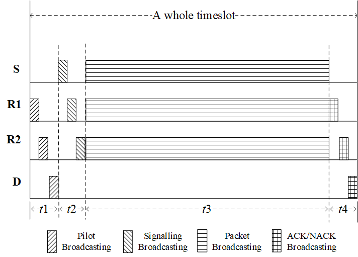
Figure 2: Timeslot model

Let

$$\Gamma_{th}=2^{R_{0}}-1$$ (9)

be the network SNR threshold, where $R_{0}$ represents the target data transmitting rate.

In our system, a whole timeslot is divided into four sub slots as shown in Fig. 2, where a whole time slot consists of pilot broadcasting sub-slot $t$1, signalling broadcasting sub-slot $t$2, packet broadcasting sub-slot $t$3 and positive acknowledgement (ACK) or negative acknowledgement (NACK) broadcasting sub-slot $t$4. In sub-slot $t$1, node D and relay nodes R1 and R2 need to broadcast the pilot signals sequentially, allowing each node to determine the CSI between itself and other nodes. Moreover, the pilot signal of D carries the overall SNR $\gamma_{overall}$ of the current received packet combined by the MRC technique so that S, R1, and R2 nodes can know the current SNR threshold $\Gamma_{th}-\gamma_{overall}$. About $\gamma_{overall}$ is descibed in OR protocol. In sub-slot $t$2, each node determines whether it is able to transmit the packet depending on its energy state, CSI and ownership of the packet. If the node can transmit the packet, then it broadcasts high-level signalling; otherwise, it broadcasts low-level signalling. And the order of S, R1, and R2 signalling broadcasting is shown in Fig. 2. In this way, each node can obtain the transmission state of the cooperative network. In sub-slot $t$3, with the transmission state, nodes determine whether transmit the packet or not based on the OR protocol described below. Then only one node can broadcast the packet in sub-slot $t$3. The blocks of sub-slot $t$3 shown in Fig. 2 just means that S, R1, and R2 are all able to broadcast packet in sub-slot $t$3, but do not mean that they can broadcast packet at the same timeslot. In sub-slot $t$4, D, R1, and R2 send a positive acknowledgment or a negative acknowledgment to indicate their reception statuses. Only when the instantaneous link SNR at the receiving node is not less than the threshold $\Gamma_{th}$, ACK signals would be broadcasted by the receiving node as the sign of successful packet reception.

II-B OR Protocol

In this part, the main steps implemented by the OR protocol are described. S, R1, and R2 are broadcast nodes. There can be more than one broadcast node as transmitter candidates (TC) at the same time which have the packet. TC set at the $i$-th timeslot is denoted by TCs$(i)$. The node which can receive the signals transmitted by the broadcast node is named the neighboring node of the broadcast node. Thus, in this system, neighboring nodes of S are R1, R2, and D, while neighboring nodes of R1 are R2 and D, and the neighboring node of R2 is D. Then, we assumed each broadcast node knows the perfect CSI of communication links between itself and each of its neighboring nodes by pilot broadcasting. Our cooperative network also assumes that S always has the packet to be transmitted. And if the signals with strong enough SNR, which is more than the current threshold, are transmitted to D, S will be set as the next broadcast node to transmit the new signals, and relay nodes clear data cache, which is indicated that one delivery is completed. Additionally, when transmitting the same packet to the same node, S has the highest transmission priority, R2 has the second priority, and R1 has the lowest priority. This is because S has fixed power support, which does not consider the energy state when transmitting packets. This way can save the harvested energy of relay nodes in order to be used in the case where only relay nodes can transmit the packet. Furthermore, the OR protocol consists of three steps:

II-B1

Determine the TCs $\textbf{S}(i)\in\{\textbf{s}_{1},\textbf{s}_{2},\textbf{s}_{3},\textbf{s}_{4},\textbf{s}_{5},\textbf{s}_{6}\}$ in the current time slot, where $\textbf{s}_{1}=\{S\}$, $\textbf{s}_{2}=\{S,R1\}$, $\textbf{s}_{3}=\{S,R2\}$, $\textbf{s}_{4}=\{(S,R1,R2)_{1}\}$, $\textbf{s}_{5}=\{(S,R1,R2)_{2}\}$, $\textbf{s}_{6}=\{(S,R1,R2)_{3}\}$. Especially, the term (S, R1, R2)₁ means the situation of the packet from R1 to R2, when both S and R1 have the packet. Term (S, R1, R2)₂ represents that the packet at R2 is from S, when both S and R1 have the packet. Term (S,R1,R2)₃ represents that S transmits the packet to R1 and R2 in the same slot.

II-B2

On the basis of the CSI between nodes, the stored energy $B_{1}(i)$ of $R1$ and the stored energy $B_{2}(i)$ of $R2$, the transmitter node $\in\{S,R1,R2,\approx\}$ is selected from the TCs $\textbf{S}(i)$, where term $\approx$ means that all nodes keep silent in the current time slot.

II-B3

Determine the effective transmission and get TCs $\textbf{S}(i+1)\in\{\textbf{s}_{1},\textbf{s}_{2},\textbf{s}_{3},\textbf{s}_{4},\textbf{s}_{5},\textbf{s}_{6}\}$ in the next time slot.

In details, all cases of OR protocol are shown in IV. Because of transmitting packets by broadcasting, D can receive all signals of the same packet to combine by MRC even in the different timeslot, no matter which the transmitter is. Therefore, we use $\gamma$ (like $\gamma_{SD}$) without $(i)$ to represent the SNR of the signal of the same packet received by D in the previous timeslot. In addition, all $\gamma(i)$ (like $\gamma_{SD}(i)$) represent the SNR of the corresponding link in the current timeslot. Assume that D received a signal with $\gamma_{1}$ SNR and a signal of the same packet with $\gamma_{2}$ SNR in the previous timeslot. After MRC technique processing, the overall SNR of the signal received by D is $\gamma_{overall}=\gamma_{1}+\gamma_{2}$. Hence, to meet the SNR threshold $\Gamma_{th}$, each node only needs to transmit the signal with $\Gamma_{th}-\gamma_{overall}$ SNR, which reduces the need for high-quality channels and improves the performance of the network. For example, when TCs$(i)$ = {S, R1}, the $\gamma_{overall}$ is $\gamma_{SD}$ which was received by D when S transmitted the signal to R1 in the previous timeslot by broadcasting way. Terms $\gamma_{overall1}$, $\gamma_{overall2}$ and $\gamma_{overall3}$ represent the SNR, which has been received by D, when TCs$(i)$ = {S, R1}, TCs$(i)$ = {S, R2} and TCs$(i)$ = {S, R1, R2} respectively. Obviously, $\gamma_{overall1}$, $\gamma_{overall2}$ and $\gamma_{overall3}$ are less than $\Gamma_{th}$.

TABLE IV: The OR Protocol

In the current time slot, the protocol determines the transmitter node and effective transmission according to the known transmitter candidates set TCs(i) and the known conditions (energy information stored by relay nodes, the current channel information, and the overall SNR of the current packet which has been combined by MRC technique), and further obtains the TCs(i + 1) of the next time slot. $TCs(i)$ transmitter effective transmission conditions $TCs(i+1)$ S S S→D $\gamma_{SD}(i)\geq\Gamma_{th}$ S S S→R1,R2 $\gamma_{SR1}(i)\geq\Gamma_{th}$,$\gamma_{SR2}(i)\geq\Gamma_{th},\gamma_{SD}(i)<\Gamma_{th}$ (S,R1,R2)₃ S S→R2 $\gamma_{SR2}(i)\geq\Gamma_{th},\gamma_{SR1}(i)<\Gamma_{th},\gamma_{SD}(i)<\Gamma_{th}$ S,R2 S S→R1 $\gamma_{SR1}(i)\geq\Gamma_{th},\gamma_{SR2}(i)<\Gamma_{th},\gamma_{SD}(i)<\Gamma_{th}$ S,R1 $\approx$ $\approx$ others S S,R1 S S→D $\gamma_{overall1}+\gamma_{SD}(i)\geq\Gamma_{th}$ S R1 R1→D $\gamma_{overall1}+\gamma_{R1D}(i)\geq\Gamma_{th},B_{1}(i)\geq M_{R1},\gamma_{overall1}+\gamma_{SD}(i)<\Gamma_{th}$ S S S→R2 $\gamma_{SR2}(i)\geq\Gamma_{th},\gamma_{overall1}+\gamma_{R1D}(i)<\Gamma_{th},B_{1}(i)\geq M_{R1},$ (S,R1,R2)₁ $\gamma_{overall1}+\gamma_{SD}(i)<\Gamma_{th}$ S S→R2 $\gamma_{SR2}(i)\geq\Gamma_{th},B_{1}(i)<M_{R1},\gamma_{overall1}+\gamma_{SD}(i)<\Gamma_{th}$ (S,R1,R2)₁ R1 R1→R2 $\gamma_{R1R2}(i)\geq\Gamma_{th},\gamma_{SR2}(i)<\Gamma_{th},B_{1}(i)\geq M_{R1},$ (S,R1,R2)₂ $\gamma_{overall1}+\gamma_{SD}(i)<\Gamma_{th}$ $\approx$ $\approx$ others S,R1 S,R2 S S→D $\gamma_{overall2}+\gamma_{SD}(i)\geq\Gamma_{th}$ S R2 R2→D $\gamma_{overall2}+\gamma_{R2D}(i)\geq\Gamma_{th},\gamma_{overall2}+\gamma_{SD}(i)<\Gamma_{th}$ S $\approx$ $\approx$ others S,R2 (S,R1,R2)₁ S S→D $\gamma_{overall3}+\gamma_{SD2}(i)\geq\Gamma_{th},B_{2}(i)\geq M_{R2}$ S R1 R1→D $\gamma_{overall3}+\gamma_{R1D}(i)\geq\Gamma_{th},\gamma_{overall3}+\gamma_{R2D}(i)<\Gamma_{th},$ S $\gamma_{overall3}+\gamma_{SD}(i)<\Gamma_{th},B_{1}(i)\geq M_{R1}$ R2 R2→D $\gamma_{SD}+\gamma_{R1D}+\gamma_{R2D}(i)\geq\Gamma_{th},$ S $\gamma_{overall3}+\gamma_{SD}(i)<\Gamma_{th},B_{2}(i)\geq M_{R2}$ $\approx$ $\approx$ others (S,R1,R2)₁ (S,R1,R2)₂ S S→D $\gamma_{overall3}+\gamma_{SD}(i)\geq\Gamma_{th}$ S R1 R1→D $\gamma_{overall3}+\gamma_{R1D}(i)\geq\Gamma_{th},\gamma_{overall3}+\gamma_{R2D}(i)\geq\Gamma_{th},$ S $\gamma_{overall3}+\gamma_{SD}(i)<\Gamma_{th}$ R2 R2→D $\gamma_{overall3}+\gamma_{R2D}(i)\geq\Gamma_{th},\gamma_{overall3}+\gamma_{SD}(i)<\Gamma_{th}$ S $\approx$ $\approx$ others (S,R1,R2)₂ (S,R1,R2)₃ S S→D $\gamma_{overall3}+\gamma_{SD}(i)\geq\Gamma_{th}$ S R1 R1→D $\gamma_{overall3}+\gamma_{R1D}(i)\geq\Gamma_{th},\gamma_{overall3}+\gamma_{R2D}(i)<\Gamma_{th},$ S $\gamma_{overall3}+\gamma_{SD}(i)<\Gamma_{th}$ R2 R2→D $\gamma_{overall3}+\gamma_{R2D}(i)\geq\Gamma_{th},\gamma_{overall3}+\gamma_{SD}(i)<\Gamma_{th}$ S $\approx$ $\approx$ others (S,R1,R2)₃

III Limiting Distribution of Energy

In this section, the expressions for the limiting distributions of energy in the PEB of R1 and R2, assuming it to be of infinite size, are derived and analyzed. The input harvest energy $X(i)$ in the $i$-th time slot is assumed to be an exponentially distributed random variable with probability density function (PDF) $f_{X}(x)$. With the mean $\mathbb{E}[X(i)]=1/\lambda$, the PDF of $X(i)$ can be expressed as

$$f_{X}(x)=\lambda e^{-\lambda x},\quad x>0.$$ (10)

Obviously, the energy harvesting parameter $\lambda$ of R1 and R2 are independent. Thus, let $\lambda_{1}$ represent the parameter of R1, and $\lambda_{2}$ represent the parameter of R2.

In order to clearly describe the theoretical derivation process, letters ’$\mathfrak{c}$’, ’$\mathfrak{d}$’, ’$\mathfrak{f}$’, ’$\mathfrak{g}$’, ’$\mathfrak{m}$’, ’$\mathfrak{n}$’ and ’$\mathfrak{o}$’ are used, whose upper cases represent conditions and lower cases represent corresponding probability values. For example,

$$\begin{split}\mathbb{C}&\triangleq\gamma_{overall1}+\gamma_{SD2}(i)<\Gamma_{th},\end{split}$$ (11)

$$\begin{split}&\mathrm{Pr}\{\gamma_{overall1}+\gamma_{SD}(i)<\Gamma_{th}\}=\mathrm{Pr}\{\mathbb{C}\}=\mathfrak{c}\\ \end{split}$$ (12)

Case-$\mathbb{C}$ means the D node receives a signal from the S node first, but the SNR of the signal is less than the threshold. Furthermore, after some slots, D receives the signal from S again, while after the MRC algorithm combines the signals, the sum of SNR is still less than the threshold. And, obviously, $\overline{\mathbb{C}}$ means the sum of SNR is greater than or equal to the threshold as well as $\overline{\mathbb{C}}=1-\mathfrak{c}$.

TABLE V: All failure transmission case only considering CSI in system table

$TCs(I)$	transmitter	recevier	condition	alias
S	S	D	$\gamma_{SD}(i)<\Gamma_{th}$	$\mathbb{A}$
	S	R1,R2	$\gamma_{SR1}(i)<\Gamma_{th}$,$\gamma_{SR2}(i)<\Gamma_{th}$	$\mathbb{B}$
	S	R2	$\gamma_{SR2}(i)<\Gamma_{th}$	$\mathbb{Q}$
	S	R1	$\gamma_{SR1}(i)<\Gamma_{th}$	$\mathbb{R}$
S,R1	S	D	$\gamma_{overall1}+\gamma_{SD}(i)<\Gamma_{th}$	$\mathbb{C}$
	R1	D	$\gamma_{overall1}+\gamma_{R1D}(i)<\Gamma_{th}$	$\mathbb{D}$
	S	R2	$\gamma_{SR2}<\Gamma_{th}$	$\mathbb{S}$
	R1	R2	$\gamma_{R1R2}<\Gamma_{th}$	$\mathbb{T}$
S,R2	S	D	$\gamma_{overall2}+\gamma_{SD}(i)<\Gamma_{th}<\Gamma_{th}$	$\mathbb{M}$
	R2	D	$\gamma_{overall2}+\gamma_{R2D}(i)<\Gamma_{th}$	$\mathbb{N}$
(S,R1,R2)1	S	D	$\gamma_{overall3}+\gamma_{SD}(i)<\Gamma_{th}$	$\mathbb{O}$
	R1	D	$\gamma_{overall3}+\gamma_{R1D}(i)<\Gamma_{th}$	$\mathbb{G}$
	R2	D	$\gamma_{overall3}+\gamma_{R2D}(i)<\Gamma_{th}$	$\mathbb{F}$
(S,R1,R2)2	S	D	$\gamma_{overall3}+\gamma_{SD}(i)<\Gamma_{th}$	$\mathbb{O}$
	R1	D	$\gamma_{overall3}+\gamma_{R1D}(i)<\Gamma_{th}$	$\mathbb{G}$
	R2	D	$\gamma_{overall3}+\gamma_{R2D}(i)<\Gamma_{th}$	$\mathbb{F}$
(S,R1,R2)3	S	D	$\gamma_{overall3}+\gamma_{SD}(i)<\Gamma_{th}$	$\mathbb{O}$
	R1	D	$\gamma_{overall3}+\gamma_{R1D}(i)<\Gamma_{th}$	$\mathbb{G}$
	R2	D	$\gamma_{overall3}+\gamma_{R2D}(i)<\Gamma_{th}$	$\mathbb{F}$

In TABLE V, all alias are shown.

Then, we can similarly get

$$\begin{split}\mathbb{D}&\triangleq\gamma_{overall1}+\gamma_{R1D}(i)<\Gamma_{th},\end{split}$$ (13)

$$\begin{split}\mathbb{F}&\triangleq\gamma_{overall3}+\gamma_{R2D}(i)<\Gamma_{th},\end{split}$$ (14)

$$\begin{split}\mathbb{G}&\triangleq\gamma_{overall3}+\gamma_{R1D2}(i)<\Gamma_{th},\end{split}$$ (15)

$$\begin{split}\mathbb{M}&\triangleq\gamma_{overall2}+\gamma_{R2D}(i)<\Gamma_{th},\end{split}$$ (16)

$$\begin{split}\mathbb{N}&\triangleq\gamma_{overall2}+\gamma_{R2D}(i)<\Gamma_{th},\end{split}$$ (17)

$$\begin{split}\mathbb{O}&\triangleq\gamma_{overall3}+\gamma_{SD2}(i)<\Gamma_{th},\end{split}$$ (18)

To obtain the expressions for PDF of energy in the PEB of R1 and R2, the probability of the transmitter candidate state needs to be calculated in advance. In [17], we know, by using the state transition matrix (STM) T of two adjacent time slots, each transmitter candidate state occurrence probabilities, $p_{s}=\mathrm{Pr}\{TCs=\{S\}\}$, $p_{SR1}=\mathrm{Pr}\{TCs=\{S,R1\}\}$, $p_{SR2}=\mathrm{Pr}\{TCs=\{S,R2\}\}$, $p_{1}=\mathrm{Pr}\{P1\}$, $p_{2}=\mathrm{Pr}\{P2\}$ and $p_{3}=\mathrm{Pr}\{P3\}$, can be updated iteratively until they converge to get their thoerical value, where $P1$ represents (S,R1,R2)₁, $P2$ represents (S,R1,R2)₂, $P3$ represents (S,R1,R2)₃. Obviously, $p_{1}+p_{2}+p_{3}=p_{SR1R2}=\mathrm{Pr}\{TCs=\{S,R1,R2\}\}$. And the STM T can be constructed as follows

$$\textbf{T}=\begin{bmatrix}p_{S-S}&p_{S-SR1}&p_{S-SR2}&p_{S-(SR1R2)_{1}}&p_{S-(SR1R2)_{2}}&p_{S-(SR1R2)_{3}}\\ p_{SR1-S}&p_{SR1-SR1}&p_{SR1-SR2}&p_{SR1-(SR1R2)_{1}}&p_{SR1-(SR1R2)_{2}}&p_{SR1-(SR1R2)_{3}}\\ p_{SR2-S}&p_{SR2-SR1}&p_{SR2-SR2}&p_{SR2-(SR1R2)_{1}}&p_{SR2-(SR1R2)_{2}}&p_{SR2-(SR1R2)_{3}}\\ p_{(SR1R2)_{1}-S}&p_{(SR1R2)_{1}-SR1}&p_{(SR1R2)_{1}-SR2}&p_{(SR1R2)_{1}-(SR1R2)_{1}}&p_{(SR1R2)_{1}-(SR1R2)_{2}}&p_{(SR1R2)_{1}-(SR1R2)_{3}}\\ p_{(SR1R2)_{2}-S}&p_{(SR1R2)_{2}-SR1}&p_{(SR1R2)_{2}-SR2}&p_{(SR1R2)_{2}-(SR1R2)_{1}}&p_{(SR1R2)_{2}-(SR1R2)_{2}}&p_{(SR1R2)_{2}-(SR1R2)_{3}}\\ p_{(SR1R2)_{3}-S}&p_{(SR1R2)_{3}-SR1}&p_{(SR1R2)_{3}-SR2}&p_{(SR1R2)_{3}-(SR1R2)_{1}}&p_{(SR1R2)_{3}-(SR1R2)_{2}}&p_{(SR1R2)_{3}-(SR1R2)_{3}}\\ \end{bmatrix},$$ (19)

where the element

$p_{i-j}(i,j\in\{S,SR1,SR2,(SR1R2)_{1},(SR1R2)_{2},(SR1R2)_{3}\})$ represents the probability that the transmitter candidate state changes from state $i$ at the current time slot to state $j$ at the next time slot, satisfying $\begin{matrix}\sum_{j\in\{S,SR1,SR2,(SR1R2)_{1},(SR1R2)_{2},(SR1R2)_{3}\}}p_{i-j}\end{matrix}=1$. The details of the algorithm for the STM-based theoretical solutions of the transmitter candidate state probability can be seen in [17]. According to the OR protocol introduced in section II, we have

$$\begin{split}p_{S-S}&=\mathrm{Pr}\{\gamma_{SD}(i)<\Gamma_{th},\gamma_{SR2}(i)<\Gamma_{th},\gamma_{SR1}(i)<\Gamma_{th}\}\\ &\quad+\mathrm{Pr}\{\gamma_{SD}(i)\geq\Gamma_{th}\}\\ &=\left(1-e^{-W_{SD}\Gamma_{th}}\right)\left(1-e^{-W_{SR2}\Gamma_{th}}\right)\left(1-e^{-W_{SR1}\Gamma_{th}}\right)\\ &\quad+e^{-W_{SD}\Gamma_{th}},\end{split}$$ (20)

$$\begin{split}p_{S-SR1}&=\mathrm{Pr}\{\gamma_{SD}(i)<\Gamma_{th},\gamma_{SR2}(i)<\Gamma_{th},\gamma_{SR1}(i)\geq\Gamma_{th}\}\\ &=\left(1-e^{-W_{SD}\Gamma_{th}}\right)\left(1-e^{-W_{SR2}\Gamma_{th}}\right)e^{-W_{SR1}\Gamma_{th}},\end{split}$$ (21)

$$\begin{split}p_{S-SR2}&=\mathrm{Pr}\{\gamma_{SD}(i)<\Gamma_{th},\gamma_{SR1}(i)<\Gamma_{th},\gamma_{SR2}(i)\geq\Gamma_{th}\}\\ &=\left(1-e^{-W_{SD}\Gamma_{th}}\right)\left(1-e^{-W_{R1D}\Gamma_{th}}\right)e^{-W_{SR2}\Gamma_{th}},\end{split}$$ (22)

$$\begin{split}p_{S-(SR1R2)_{3}}&=\mathrm{Pr}\{\gamma_{SD}(i)<\Gamma_{th},\gamma_{SR1}(i)\geq\Gamma_{th},\\ &\qquad\gamma_{SR2}(i)\geq\Gamma_{th}\}\\ &=\left(1-e^{-W_{SD}\Gamma_{th}}\right)e^{-W_{R1D}\Gamma_{th}}e^{-W_{SR2}\Gamma_{th}},\end{split}$$ (23)

$$\begin{split}p_{SR1-S}&=\mathrm{Pr}\{\overline{\mathbb{C}}\}+\mathrm{Pr}\{B_{1}(i)\geq M_{R1},\mathbb{C},\overline{\mathbb{D}}\}\\ &=(1-\mathfrak{c})+\mathfrak{c}*PU1*(1-\mathfrak{d}),\end{split}$$ (24)

$$\begin{split}p_{SR1-(SR1R2)_{1}}&=\mathrm{Pr}\{\mathbb{C},B_{1}(i)\geq M_{R1},\mathbb{D},\gamma_{R1R2}(i)\geq\Gamma_{th},\\ &\quad\gamma_{SR2}(i)\geq\Gamma_{th}\}\\ &=\mathfrak{c}*PU1*\mathfrak{d}*e^{-W_{R1R2}\Gamma_{th}}*(1-^{-W_{SR2}\Gamma_{th}}),\end{split}$$ (25)

$$\begin{split}p_{SR1-(SR1R2)_{2}}&=\mathrm{Pr}\{\mathbb{C},B_{1}(i)\geq M_{R1},\mathbb{D},\gamma_{SR2}(i)\geq\Gamma_{th}\}\\ &+\mathrm{Pr}\{\mathbb{C},B_{1}(i)<M_{R1},\gamma_{R1R2}(i)\geq\Gamma_{th}\}\\ &=\mathfrak{c}*PU1*\mathfrak{d}*e^{-W_{SR2}\Gamma_{th}}+\mathfrak{c}*(1-PU1)\\ &\times e^{-W_{SR2}\Gamma_{th}},\end{split}$$ (26)

$$\begin{split}p_{SR1-SR1}&=\mathrm{Pr}\{B_{1}(i)<M_{R1},\mathbb{C}\}\\ &+\mathrm{Pr}\{B_{1}(i)\geq M_{R1},\mathbb{C},\mathbb{D},\gamma_{R1R2}(i)\geq\Gamma_{th},\\ &\gamma_{SR2}(i)\geq\Gamma_{th}\}+\mathrm{Pr}\{B_{1}(i)\geq M_{R1},\mathbb{C},\mathbb{D},\\ &\gamma_{R1R2}(i)<\Gamma_{th},\gamma_{SR2}(i)<\Gamma_{th}\}\\ &=1-p_{SR1-(SR1R2)_{1}}-p_{SR1-S}-p_{SR1-(SR1R2)_{2}},\end{split}$$ (27)

$$\begin{split}p_{SR2-S}&=\mathrm{Pr}\{\overline{\mathbb{M}}\}+\mathrm{Pr}\{B_{2}(i)\geq M_{R2},\mathbb{M},\overline{\mathbb{N}}\}\\ &=(1-\mathfrak{m})+PU2*\mathfrak{m}*(1-\mathfrak{n}),\end{split}$$ (28)

$$\begin{split}p_{SR2-SR2}&=\mathrm{Pr}\{B_{2}(i)\geq M_{R2},\mathbb{M},\mathbb{N}\}+\mathrm{Pr}\{B_{2}(i)<M_{R2}\}\\ &=1-p_{SR2-S},\end{split}$$ (29)

$$\begin{split}p_{(SR1R2)_{1}-S}&=\mathrm{Pr}\{\overline{\mathbb{O}}\}+\mathrm{Pr}\{\mathbb{O},B_{2}(i)\geq M_{R2},\overline{\mathbb{F}}\}\\ &+\mathrm{Pr}\{\mathbb{O},B_{2}(i)\geq M_{R2},\mathbb{F},B_{1}(i)\geq M_{R1},\overline{\mathbb{G}}\}\\ &+\mathrm{Pr}\{\mathbb{O},B_{2}(i)<M_{R2},B_{1}(i)\geq M_{R1},\overline{\mathbb{G}}\}\\ &=(1-\mathfrak{o})+\mathfrak{o}*(PU2*(1-\mathfrak{f})\\ &+(PU2*\mathfrak{f}+(1-PU2))*PU1*(1-\mathfrak{g})),\end{split}$$ (30)

$$\begin{split}p_{(SR1R2)_{1}-(SR1R2)_{1}}&=1-p_{(SR1R2)_{1}-S},\end{split}$$ (31)

$$\begin{split}p_{(SR1R2)_{2}-S}&=\mathrm{Pr}\{\overline{\mathbb{O}}\}+\mathrm{Pr}\{\mathbb{O},B_{2}(i)\geq M_{R2},\overline{\mathbb{F}}\}\\ &+\mathrm{Pr}\{\mathbb{O},B_{2}(i)\geq M_{R2},\mathbb{F},B_{1}(i)\geq M_{R1},\overline{\mathbb{G}}\}\\ &+\mathrm{Pr}\{\mathbb{O},B_{2}(i)<M_{R2},B_{1}(i)\geq M_{R1},\overline{\mathbb{G}}\}\\ &=(1-\mathfrak{o})+\mathfrak{o}*(PU2*(1-\mathfrak{f})\\ &+(PU2*\mathfrak{f}+(1-PU2))*PU1*(1-\mathfrak{g})),\end{split}$$ (32)

$$\begin{split}p_{(SR1R2)_{2}-(SR1R2)_{2}}&=1-p_{(SR1R2)_{2}-S},\end{split}$$ (33)

$$\begin{split}p_{(SR1R2)_{3}-S}&=\mathrm{Pr}\{\overline{\mathbb{O}}\}+\mathrm{Pr}\{\mathbb{O},B_{2}(i)\geq M_{R2},\overline{\mathbb{F}}\}\\ &+\mathrm{Pr}\{\mathbb{O},B_{2}(i)\geq M_{R2},\mathbb{F},B_{1}(i)\geq M_{R1},\overline{\mathbb{G}}\}\\ &+\mathrm{Pr}\{\mathbb{O},B_{2}(i)<M_{R2},B_{1}(i)\geq M_{R1},\overline{\mathbb{G}}\}\\ &=(1-\mathfrak{o})+\mathfrak{o}*(PU2*(1-\mathfrak{f})\\ &+(PU2*\mathfrak{f}+(1-PU2))*PU1*(1-\mathfrak{g})),\end{split}$$ (34)

$$\begin{split}p_{(SR1R2)_{3}-(SR1R2)_{3}}&=1-p_{(SR1R2)_{3}-S},\end{split}$$ (35)

where, $PU1=\frac{1}{b_{1}\lambda_{1}M_{R1}}$ and $PU2=\frac{1}{b_{2}\lambda_{2}M_{R2}}$. $b_{1}$ and $b_{2}$ are given in (65) and (58). And the proof of $PU1$ and $PU2$ are given in (75) and (77). And the remaining elements of T are equal to 0.

In order to get T, the values of $c$, $\mathfrak{d}$, $\mathfrak{f}$, $g$, $m$, $n$ and $o$ are required. Before this step, it is foundation to get the probability distributions $p_{\gamma_{overall1}}(j)$, $p_{\gamma_{overall2}}(j)$, $p_{\gamma_{overall3}}(j)$ of $\gamma_{overall1}$, $\gamma_{overall2}$ and $\gamma_{overall3}$. For example, $p_{\gamma_{overall1}}(j)$ is the probability that node D has received the SNR of value $(\frac{j-1}{\mathcal{N}}\Gamma_{th}\leq\gamma_{overall1}<\frac{j}{\mathcal{N}}\Gamma_{th})$ when TCs = $\{S,R1\}$. To obtain these probability distributions, the STM method is used. STM T1, STM T2 and STM T3 correspond to $p_{\gamma_{overall1}}$, $p_{\gamma_{overall2}}$ and $p_{\gamma_{overall3}}$ respectively. The size of T1 is $\mathcal{N}$ $\times$ $\mathcal{N}$ dimension. The states of T1 are the value of $\gamma_{overall1}$ and the element $\textbf{T1}(i,j)$ means the transition probability from $(\frac{i-1}{\mathcal{N}}\Gamma_{th}\leq\gamma_{overall1}<\frac{i}{\mathcal{N}}\Gamma_{th})$ to $(\frac{j-1}{\mathcal{N}}\Gamma_{th}\leq\gamma_{overall1}<\frac{j}{\mathcal{N}}\Gamma_{th})$, where $1\leq i,j\leq\mathcal{N}$ and $i,j\in Z$. The elements of T1 are as follows:

$$\begin{split}\textbf{T1}(i,j)&=(1-\int_{0}^{\frac{\mathcal{N}-i}{\mathcal{N}}\Gamma_{th}}f_{SD}(x)dx\\ &\times(PU1\int_{0}^{\frac{\mathcal{N}-i}{\mathcal{N}}\Gamma_{th}}f_{R1D}(x)dx\\ &\times\int_{0}^{\Gamma_{th}}f_{SR2}(x)dx\int_{0}^{\Gamma_{th}}f_{R1R2}(x)dx\\ &+(1-PU1)\int_{0}^{\Gamma_{th}}f_{SR2}(x)dx))\\ &\times\int_{\frac{j-1}{\mathcal{N}}\Gamma_{th}}^{\frac{j}{\mathcal{N}}\Gamma_{th}}f_{SD}(x)dx/\int_{0}^{\Gamma_{th}}f_{SD}(x)dx\\ &\qquad\qquad\qquad\qquad\qquad\qquad\qquad\quad i\neq j\end{split}$$ (36)

$$\begin{split}\textbf{T1}(i,j)&=(1-\int_{0}^{\frac{\mathcal{N}-i}{\mathcal{N}}\Gamma_{th}}f_{SD}(x)dx\\ &\times(PU1\int_{0}^{\frac{\mathcal{N}-i}{\mathcal{N}}\Gamma_{th}}f_{R1D}(x)dx\\ &\times\int_{0}^{\Gamma_{th}}f_{SR2}(x)dx\int_{0}^{\Gamma_{th}}f_{R1R2}(x)dx\\ &+(1-PU1)\int_{0}^{\Gamma_{th}}f_{SR2}(x)dx))\\ &\times\int_{\frac{j-1}{\mathcal{N}}\Gamma_{th}}^{\frac{j}{\mathcal{N}}\Gamma_{th}}f_{SD}(x)dx/\int_{0}^{\Gamma_{th}}f_{SD}(x)dx\\ &+\int_{0}^{\frac{\mathcal{N}-i}{\mathcal{N}}\Gamma_{th}}f_{SD}(x)dx\\ &\times(PU1\int_{0}^{\frac{\mathcal{N}-i}{\mathcal{N}}\Gamma_{th}}f_{R1D}(x)dx\\ &\times\int_{0}^{\Gamma_{th}}f_{SR2}(x)dx\int_{0}^{\Gamma_{th}}f_{R1R2}(x)dx\\ &+(1-PU1)\int_{0}^{\Gamma_{th}}f_{SR2}(x)dx)\\ &\qquad\qquad\qquad\qquad\qquad\qquad\qquad\quad i=j\end{split}$$ (37)

Similarly, the elements of T2 and T3 are as follows:

$$\begin{split}\textbf{T2}(i,j)&=(1-\int_{0}^{\frac{\mathcal{N}-i}{\mathcal{N}}\Gamma_{th}}f_{SD}(x)dx\\ &\times(PU2\int_{0}^{\frac{\mathcal{N}-i}{\mathcal{N}}\Gamma_{th}}f_{R2D}(x)dx+(1-PU2)))\\ &\times\int_{\frac{j-1}{\mathcal{N}}\Gamma_{th}}^{\frac{j}{\mathcal{N}}\Gamma_{th}}f_{SD}(x)dx/\int_{0}^{\Gamma_{th}}f_{SD}(x)dx\\ &\qquad\qquad\qquad\qquad\qquad\qquad\qquad\quad i\neq j\end{split}$$ (38)

$$\begin{split}\textbf{T2}(i,j)&=(1-\int_{0}^{\frac{\mathcal{N}-i}{\mathcal{N}}\Gamma_{th}}f_{SD}(x)dx\\ &\times(PU2\int_{0}^{\frac{\mathcal{N}-i}{\mathcal{N}}\Gamma_{th}}f_{R2D}(x)dx+(1-PU2)))\\ &\times\int_{\frac{j-1}{\mathcal{N}}\Gamma_{th}}^{\frac{j}{\mathcal{N}}\Gamma_{th}}f_{SD}(x)dx/\int_{0}^{\Gamma_{th}}f_{SD}(x)dx\\ &+\int_{0}^{\frac{\mathcal{N}-i}{\mathcal{N}}\Gamma_{th}}f_{SD}(x)dx\\ &\times(PU2\int_{0}^{\frac{\mathcal{N}-i}{\mathcal{N}}\Gamma_{th}}f_{R2D}(x)dx+(1-PU2))\\ &\qquad\qquad\qquad\qquad\qquad\qquad\qquad\quad i=j\end{split}$$ (39)

$$\begin{split}\textbf{T3}(i,j)&=(1-\int_{0}^{\frac{\mathcal{N}-i}{\mathcal{N}}\Gamma_{th}}f_{SD}(x)dx\\ &\times(PU2\int_{0}^{\frac{\mathcal{N}-i}{\mathcal{N}}\Gamma_{th}}f_{R2D}(x)dx+(1-PU2))\\ &\times(PU1\int_{0}^{\frac{\mathcal{N}-i}{\mathcal{N}}\Gamma_{th}}f_{R1D}(x)dx+(1-PU1)))\\ &\times(\frac{p_{3}}{p_{1}+p_{2}+p_{3}}\frac{\int_{\frac{j-1}{\mathcal{N}}\Gamma_{th}}^{\frac{j}{\mathcal{N}}\Gamma_{th}}f_{SD}(x)dx}{\int_{0}^{\Gamma_{th}}f_{SD}(x)dx}\\ &+\frac{p_{2}}{p_{1}+p_{2}+p_{3}}\frac{p_{d_{S->R2}}(j)}{\sum_{k=1}^{\mathcal{N}}p_{d_{S->R2}}(k)}\\ &+\frac{p_{1}}{p_{1}+p_{2}+p_{3}}\frac{p_{d_{R1->R2}}(j)}{\sum_{k=1}^{\mathcal{N}}p_{d_{R1->R2}}(k)})\\ &\qquad\qquad\qquad\qquad\qquad\qquad\qquad\quad i\neq j\end{split}$$ (40)

$$\begin{split}\textbf{T3}(i,j)&=(1-\int_{0}^{\frac{\mathcal{N}-i}{\mathcal{N}}\Gamma_{th}}f_{SD}(x)dx\\ &\times(PU2\int_{0}^{\frac{\mathcal{N}-i}{\mathcal{N}}\Gamma_{th}}f_{R2D}(x)dx+(1-PU2))\\ &\times(PU1\int_{0}^{\frac{\mathcal{N}-i}{\mathcal{N}}\Gamma_{th}}f_{R1D}(x)dx+(1-PU1)))\\ &\times(\frac{p_{3}}{p_{1}+p_{2}+p_{3}}\frac{\int_{\frac{j-1}{\mathcal{N}}\Gamma_{th}}^{\frac{j}{\mathcal{N}}\Gamma_{th}}f_{SD}(x)dx}{\int_{0}^{\Gamma_{th}}f_{SD}(x)dx}\\ &+\frac{p_{2}}{p_{1}+p_{2}+p_{3}}\frac{p_{d_{S->R2}}(j)}{\sum_{k=1}^{\mathcal{N}}p_{d_{S->R2}}(k)}\\ &+\frac{p_{1}}{p_{1}+p_{2}+p_{3}}\frac{p_{d_{R1->R2}}(j)}{\sum_{k=1}^{\mathcal{N}}p_{d_{R1->R2}}(k)})\\ &+\int_{0}^{\frac{\mathcal{N}-i}{\mathcal{N}}\Gamma_{th}}f_{SD}(x)dx\\ &\times(PU2\int_{0}^{\frac{\mathcal{N}-i}{\mathcal{N}}\Gamma_{th}}f_{R2D}(x)dx+(1-PU2))\\ &\times(PU1\int_{0}^{\frac{\mathcal{N}-i}{\mathcal{N}}\Gamma_{th}}f_{R1D}(x)dx+(1-PU1)))\\ &\qquad\qquad\qquad\qquad\qquad\qquad\qquad\quad i=j\end{split}$$ (41)

where $p_{d_{S->R2}}(j)$ is the probability that node D receives the SNR of value $(\frac{j-1}{\mathcal{N}}\Gamma_{th}\leq\gamma_{overall1}+\gamma_{SD}<\frac{j}{\mathcal{N}}\Gamma_{th})$ when system has transitioned the TCs state from $\{S,R1\}$ to $\{S,R1,R2\}_{1}$, while $p_{d_{R1->R2}}(j)$ is the probability that node D receives the SNR of value $(\frac{j-1}{\mathcal{N}}\Gamma_{th}\leq\gamma_{overall1}+\gamma_{R1D}<\frac{j}{\mathcal{N}}\Gamma_{th})$ when system has transitioned the TCs state from $\{S,R1\}$ to $\{S,R1,R2\}_{2}$. Obviously, the expressions of $p_{d_{S->R2}}(j)$ and $p_{d_{R1->R2}}(j)$ are as follows:

$$\begin{split}p_{d_{S->R2}}(j)=\mathrm{conv}(p_{\gamma_{overall1}},p_{SD})\\ \end{split}$$ (42)

$$\begin{split}p_{d_{R1->R2}}(j)=\mathrm{conv}(p_{\gamma_{overall1}},p_{R1D})\\ \end{split}$$ (43)

where

$$\begin{split}p_{SD}(j)=\int_{\frac{j-1}{\mathcal{N}}\Gamma_{th}}^{\frac{j}{\mathcal{N}}\Gamma_{th}}f_{SD}(x)dx\\ \end{split}$$ (44)

$$\begin{split}p_{R1D}(j)=\int_{\frac{j-1}{\mathcal{N}}\Gamma_{th}}^{\frac{j}{\mathcal{N}}\Gamma_{th}}f_{R1D}(x)dx.\\ \end{split}$$ (45)

Similarly,

$$\begin{split}p_{R2D}(j)=\int_{\frac{j-1}{\mathcal{N}}\Gamma_{th}}^{\frac{j}{\mathcal{N}}\Gamma_{th}}f_{R2D}(x)dx.\\ \end{split}$$ (46)

With these parameter, the expressions of $c$, $\mathfrak{d}$, $\mathfrak{f}$, $g$, $m$, $n$ and $o$ can be derived.

$$\begin{split}\mathfrak{c}=\sum_{j=1}^{\mathcal{N}}\mathrm{conv}(p_{\gamma_{overall1}},p_{SD})\end{split}$$ (47)

$$\begin{split}\mathfrak{d}=\sum_{j=1}^{\mathcal{N}}\mathrm{conv}(p_{\gamma_{overall1}},p_{R1D})\end{split}$$ (48)

$$\begin{split}\mathfrak{m}=\sum_{j=1}^{\mathcal{N}}\mathrm{conv}(p_{\gamma_{overall2}},p_{SD})\end{split}$$ (49)

$$\begin{split}\mathfrak{n}=\sum_{j=1}^{\mathcal{N}}\mathrm{conv}(p_{\gamma_{overall2}},p_{R2D})\end{split}$$ (50)

$$\begin{split}\mathfrak{f}=\sum_{j=1}^{\mathcal{N}}\mathrm{conv}(p_{\gamma_{overall3}},p_{R2D})\end{split}$$ (51)

$$\begin{split}\mathfrak{g}=\sum_{j=1}^{\mathcal{N}}\mathrm{conv}(p_{\gamma_{overall3}},p_{R1D})\end{split}$$ (52)

$$\begin{split}\mathfrak{o}=\sum_{j=1}^{\mathcal{N}}\mathrm{conv}(p_{\gamma_{overall3}},p_{SD})\end{split}$$ (53)

The detailed process for obtaining probability $p_{s}$, $p_{SR1}$, $p_{SR2}$, $p_{1}$, $p_{2}$, $p_{3}$, $p_{\gamma_{overall1}}(j)$, $p_{\gamma_{overall2}}(j)$, $p_{\gamma_{overall3}}(j)$, ’$\mathfrak{c}$’, ’$\mathfrak{d}$’, ’$\mathfrak{f}$’, ’$\mathfrak{g}$’, ’$\mathfrak{m}$’, ’$\mathfrak{n}$’ and ’$\mathfrak{o}$’ is shown in Alg. A. See Appendix A.

As the preparations are ready, in sections A and B, the PDF of energy in the PEB of R1 and R2 are obtained, respectively.

III-A Limiting Distribution of R2 Energy

By using the DCSMC and donating the energy level in the infinite-size energy buffer in the $i$-th signaling interval as $B_{2}(i)$, the PEB’s buffer of R2 update equations are given by

$$\begin{split}&B_{2}(i+1)=B_{2}(i)+X(i),\quad\mathbb{P}_{21}\\ &B_{2}(i+1)=B_{2}(i)-M_{R2}+X(i),\quad\mathbb{P}_{22}\end{split}$$ (54)

where $\mathbb{P}_{21}$ and $\mathbb{P}_{22}$ are the applicable conditions of the update equations, respectively. They are given by

$$\begin{split}\mathbb{P}_{21}:\,&\big{(}TCs=\{S\}\big{)}\cup\big{(}TCs=\{S,R1\}\big{)}\\ &\cup\Big{[}\big{(}TCs=\{S,R2\}\big{)}\cap\big{(}B_{2}(i)<M_{R2}\big{)}\Big{]}\\ &\cup\Big{[}\big{(}TCs=\{S,R2\}\big{)}\cap\big{(}B_{2}(i)\geq M_{R2}\big{)}\cap\mathbb{M}\cap\mathbb{N}\Big{]}\\ &\cup\Big{[}\big{(}TCs=\{S,R2\}\big{)}\cap\big{(}B_{2}(i)\geq M_{R2}\big{)}\cap\overline{\mathbb{M}}\Big{]}\\ &\cup\Big{[}\big{(}TCs=\{S,R1,R2\}\big{)}\cap\big{(}B_{2}(i)\geq M_{R2}\cap\mathbb{O}\cap\mathbb{F}\big{)}\Big{]}\\ &\cup\Big{[}\big{(}TCs=\{S,R1,R2\}\big{)}\cap\big{(}B_{2}(i)\geq M_{R2}\cap\overline{\mathbb{O}}\big{)}\Big{]}\\ &\cup\Big{[}\big{(}TCs=\{S,R1,R2\}\big{)}\cap\big{(}B_{2}(i)<M_{R2}\big{)}\Big{]},\end{split}$$ (55)

$$\begin{split}\mathbb{P}_{22}:\,&\Big{[}\big{(}TCs=\{S,R2\}\big{)}\cap\big{(}B_{2}(i)\geq M_{R2}\big{)}\cap\mathbb{C}\cap\overline{\mathbb{N}}\Big{]}\\ &\cup\Big{[}\big{(}TCs=\{S,R1,R2\}\big{)}\cap\big{(}B_{2}(i)\geq M_{R2}\cap\mathbb{O}\cap\overline{\mathbb{F}}\big{)}\Big{]}.\end{split}$$ (56)

Let $\psi_{R2}$ represents the energy buffer convergence parameter for the energy update process $B_{1}(i)$ of Eq. (54), with the help of the Eq. (47) to Eq. (53) , which can be expressed as follows

$$\begin{split}\psi_{R2}&=\lambda_{2}M_{R2}\Big{[}p_{SR2}*\mathfrak{m}(1-\mathfrak{n})+(p_{1}+p_{2}+p_{3})*\mathfrak{o}(1-\mathfrak{f})\Big{]}\\ &=\lambda_{2}M_{R2}b_{2},\end{split}$$ (57)

where

$$\begin{split}b_{2}&=p_{SR2}*\mathfrak{m}(1-\mathfrak{n})+(p_{1}+p_{2}+p_{3})*o(1-\mathfrak{f}).\end{split}$$ (58)

The limiting PDF when $\psi_{R2}>1$ is obtained in Theorem 1, and the scenario when $\psi_{R2}\leq 1$ is discussed in Theorem 2.

Theorem 1

If $\psi_{R2}>1$, the energy update process $B_{2}(i)$ in Eq. (54) will have a stationary distribution. Furthermore, the limiting PDF of the energy buffer state at R2 can be expressed by

$$g_{2}(x)=\begin{cases}\dfrac{1}{M_{R2}}\left(1-e^{Q_{2}x}\right),&0\leq x<M_{R2}\\ \dfrac{1}{M_{R2}}\dfrac{-Q_{2}e^{Q_{2}x}}{\left(b_{2}\lambda_{2}+Q_{2}\right)},&x\geq M_{R2}.\end{cases}$$ (59)

Where

$$\begin{split}Q_{2}=\frac{-W\left(-b_{2}\lambda_{2}M_{R2}e^{-b_{2}\lambda_{2}M_{R2}}\right)}{M_{R2}}-b_{2}\lambda_{2}<0,\end{split}$$ (60)

satisfying $b_{2}\lambda_{2}e^{Q_{2}M_{R2}}=b_{2}\lambda_{2}+Q_{2}$.

Proof 1

The proof is given in Appendix B.

Theorem 2

When $\psi_{R2}\leq 1$, there is no stationary PDF of the energy buffer state of R1. In addition, after a finite number of time slots, the R1 energy buffer will keep $B_{2}(i)>M_{R2}$.

Proof 2

The proof is given in Appendix C.

III-B Limiting Distribution of R1 Energy

Similar to the solution of the limiting distribution of R2 energy, by using the DCSMC and donating the energy level in the infinite-size energy buffer in the $i$-th signaling interval as $B_{1}(i)$, the PEB’s buffer of R1 update equations are given by

$$\begin{split}&B_{1}(i+1)=B_{1}(i)+X(i),\quad\mathbb{P}_{11}\\ &B_{1}(i+1)=B_{1}(i)-M_{R1}+X(i),\quad\mathbb{P}_{12}\end{split}$$ (61)

where $\mathbb{P}_{11}$ and $\mathbb{P}_{12}$ are the update conditions needed for the equations in Eq. (61) according to OR protocol. Correspondingly, they can be expressed as follows

$$\begin{split}\mathbb{P}_{12}:\,&\Big{[}\big{(}TCs=\{S,R1\}\big{)}\cap\big{(}B_{1}(i)\geq M_{R1}\big{)}\cap\mathbb{C}\cap\overline{\mathbb{D}}\Big{]}\\ &\cup\Big{[}\big{(}TCs=\{S,R1\}\big{)}\cap\big{(}\big{(}B_{1}(i)\geq M_{R1}\big{)},\mathbb{C},\mathbb{D},\\ &\qquad\gamma_{SR2}(i)<\Gamma_{th},\gamma_{R1R2}(i)\geq\Gamma_{th}\big{)}\Big{]}\\ &\cup\Big{[}\big{(}TCs=\{S,R1,R2\}\big{)}\cap\big{(}B_{2}(i)\geq M_{R2},\mathbb{O},\mathbb{F},\\ &\big{(}B_{1}(i)\geq M_{R1}\big{)},\overline{\mathbb{G}}\big{)}\Big{]}\\ &\cup\Big{[}\big{(}TCs=\{S,R1,R2\}\big{)}\cap\big{(}B_{2}(i)<M_{R2},\mathbb{O},\\ &\big{(}B_{1}(i)\geq M_{R1}\big{)},\overline{\mathbb{G}}\big{)}\Big{]},\end{split}$$ (62)

$$\begin{split}\mathbb{P}_{11}:\,&\big{(}TCs=\{S\}\big{)}\cup\big{(}TCs=\{S,R2\}\big{)}\\ &\cup\Big{[}\big{(}TCs=\{S,R1\}\big{)}\cap\big{(}B_{1}(i)<M_{R1}\big{)}\Big{]}\\ &\cup\Big{[}\big{(}TCs=\{S,R1\}\big{)}\cap\big{(}B_{1}(i)\geq M_{R1},\mathbb{C},\mathbb{D},\\ &\qquad\gamma_{SR2}(i)\geq\Gamma_{th},\big{)}\Big{]}\\ &\cup\Big{[}\big{(}TCs=\{S,R1\}\big{)}\cap\big{(}B_{1}(i)\geq M_{R1},\mathbb{C},\mathbb{D},\\ &\qquad\gamma_{SR2}(i)<\Gamma_{th},\gamma_{R1R2}(i)<\Gamma_{th}\big{)}\Big{]}\\ &\cup\Big{[}\big{(}P1\big{)}\cap\big{(}B_{2}(i)\geq M_{R2},\mathbb{O},\overline{\mathbb{F}}\big{)}\Big{]}\\ &\cup\Big{[}\big{(}TCs=\{S,R1,R2\}\big{)}\cap\big{(}B_{2}(i)\geq M_{R2},\mathbb{O},\mathbb{F},\\ &B_{1}(i)\geq M_{R1},\mathbb{G}\big{)}\Big{]}\\ &\cup\Big{[}\big{(}TCs=\{S,R1,R2\}\big{)}\cap\big{(}B_{2}(i)\geq M_{R2},\mathbb{O},\mathbb{F},\\ &B_{1}(i)<M_{R1}\big{)}\Big{]}\\ &\cup\Big{[}\big{(}TCs=\{S,R1,R2\}\big{)}\cap\big{(}B_{2}(i)<M_{R2},\mathbb{O},\\ &B_{1}(i)\geq M_{R1},\mathbb{G}\big{)}\Big{]}\\ &\cup\Big{[}\big{(}TCs=\{S,R1,R2\}\big{)}\cap\big{(}B_{2}(i)<M_{R2},\mathbb{O},\\ &B_{1}(i)<M_{R1}\big{)}\Big{]}.\end{split}$$ (63)

Let $\psi_{R1}$ represent the energy buffer convergence parameter for the energy update process $B_{1}(i)$ of Eq. (61), which can be expressed as follows

$$\begin{split}\psi_{R1}&=\lambda_{1}M_{R1}\Big{[}p_{SR1}*\mathfrak{c}((1-\mathfrak{d})+\mathfrak{d}(1-e^{-W_{SR2}\Gamma_{th}})e^{-W_{R1R2}\Gamma_{th}}\\ &+PU2((p_{1}+p_{2}+p_{3})*\mathfrak{o}*\mathfrak{f}(1-\mathfrak{g})\\ &+(1-PU2)*((p_{1}+p_{2}+p_{3})*\mathfrak{o}(1-\mathfrak{g}))\Big{]}\\ &=\lambda_{1}M_{R1}b_{1},\end{split}$$ (64)

where

$$\begin{split}b_{1}&=p_{SR1}*\mathfrak{c}((1-\mathfrak{d})+\mathfrak{d}(1-e^{-W_{SR2}\Gamma_{th}})e^{-W_{R1R2}\Gamma_{th}}\\ &+PU2((p_{1}+p_{2}+p_{3})*\mathfrak{o}*\mathfrak{f}(1-\mathfrak{g})\\ &+(1-PU2)*((p_{1}+p_{2}+p_{3})*\mathfrak{o}(1-\mathfrak{g})).\end{split}$$ (65)

The limiting PDF when $\psi_{R1}>1$ is obtained in Theorem 3, and the scenario when $\psi_{R1}\leq 1$ is discussed in Theorem 4.

Theorem 3

If $\psi_{1}>1$, the energy update process $B_{1}(i)$ in Eq. (61) will have a stationary distribution. Furthermore, the limiting PDF of the energy buffer state at R1 can be expressed by

$$g_{1}(x)=\begin{cases}\dfrac{1}{M_{R1}}\left(1-e^{Q_{1}x}\right),&0\leq x<M_{R1}\\ \dfrac{1}{M_{R1}}\dfrac{-Q_{1}e^{Q_{1}x}}{\left(b_{1}\lambda_{1}+Q_{1}\right)},&x\geq M_{R1}.\end{cases}$$ (66)

And

$$\begin{split}Q_{1}=\frac{-W\left(-b_{1}\lambda_{1}M_{R}e^{-b_{1}\lambda_{1}M_{R1}}\right)}{M_{R1}}-b_{1}\lambda_{1}<0,\end{split}$$ (67)

satisfying $b_{1}\lambda_{1}e^{Q_{1}M_{R1}}=b_{1}\lambda_{1}+Q_{1}$.

Proof 3

The proof is given in Appendix D.

Theorem 4

Similar to Theorem 2, when $\psi_{R1}\leq 1$, there is no stationary PDF of the energy buffer state of R1. And the energy in the R1 energy buffer keeps more than $M_{R1}$.

IV Analysis of Outage Probability and Throughput

This section focuses on the analysis of outage probability, timeslot cost, and throughput of our system, when both $B_{1}(i)$ and $B_{2}(i)$ have limiting PDFs.

According to OR protocol, when all the transmitter candidates fail to transmit signals to the D node, the communication network system is defined as an outage. In an outage, transmitter candidates can transmit the signal to other nodes. Obviously, the system outage probability (OP) can be expressed as

$$\begin{split}OP=rp_{S}+rp_{SR1}+rp_{SR2}+rp_{SR1R2},\end{split}$$ (68)

where, $rp_{S}$, $rp_{SR1}$, $rp_{SR2}$ and $rp_{SR1R2}$ are the outage probability of transmitter candidates set {S}, {S,R1}, {SR2}, {S,R1,R2}, respectively. The outage probability of the node means the transmitter candidates as the broadcast node fail to transmit signals to the D node. Specifically, they can be expressed by

$$\begin{split}rp_{S}&=p_{S}\mathrm{Pr}\{\gamma_{SD}(i)<\Gamma_{th}\}\\ &=p_{S}\left(1-e^{-W_{SD}\Gamma_{th}}\right),\end{split}$$ (69)

$$\begin{split}rp_{SR1}&=p_{SR1}[\mathrm{Pr}\{\mathbb{C},\mathbb{D},B_{1}(i)\geq M_{R1}\}\\ &+\mathrm{Pr}\{\mathbb{C},B_{1}(i)<M_{R1}\}]\\ &=p_{SR1}*\mathfrak{c}(\mathfrak{d}*PU1+1-PU1),\end{split}$$ (70)

$$\begin{split}rp_{SR2}&=p_{SR2}[\mathrm{Pr}\{\mathbb{M},\mathbb{N},B_{2}(i)\geq M_{R2}\}\\ &+\mathrm{Pr}\{\mathbb{M},B_{2}(i)<M_{R2}\}]\\ &=p_{SR2}*\mathfrak{m}(\mathfrak{n}*PU2+1-PU2),\end{split}$$ (71)

$$\begin{split}&rp_{SR1R2}\\ &=(p_{1}+p_{2}+p_{3})\Big{[}\mathrm{Pr}\{\mathbb{O},\mathbb{F},B_{2}(i)\geq M_{R2},\mathbb{G},B_{1}(i)\geq M_{R1}\}\\ &+\mathrm{Pr}\{\mathbb{O},\mathbb{F},B_{2}(i)\geq M_{R2},B_{1}(i)<M_{R1}\}\\ &+\mathrm{Pr}\{\mathbb{O},B_{2}(i)<M_{R2},\mathbb{G},B_{1}(i)\geq M_{R1}\}\\ &+\mathrm{Pr}\{\mathbb{O},B_{2}(i)<M_{R2},B_{1}(i)<M_{R1}\}\Big{]}\\ &=(p_{1}+p_{2}+p_{3})(\mathfrak{o}(\mathfrak{f}*PU2+1-PU2)\\ &\qquad\times(\mathfrak{g}*PU1+1-PU1)).\end{split}$$ (72)

With the Eq. (59), we get

$$\begin{split}\mathrm{Pr}\{B_{2}(i)<M_{R2}\}&=\int_{x=0}^{M_{R2}}\dfrac{\left(1-e^{Q_{2}x}\right)}{M_{R2}}\,dx\\ &=1-\dfrac{\left(e^{Q_{2}M_{R2}}-1\right)}{Q_{2}M_{R2}}.\end{split}$$ (73)

Due to $b_{2}\lambda_{2}e^{Q_{2}M_{R2}}=b_{2}\lambda_{2}+Q_{2}$, we get $e^{Q_{2}M_{R2}}=1+\frac{Q_{2}}{b_{2}\lambda_{2}}$, and thus

$$\begin{split}\mathrm{Pr}\{B_{2}(i)<M_{R2}\}&=1-\dfrac{\left(1+\frac{Q_{2}}{b_{2}\lambda_{2}}-1\right)}{Q_{2}M_{R2}}\\ &=1-\dfrac{1}{b_{2}\lambda_{2}M_{R2}}.\end{split}$$ (74)

Accordingly, we get

$$\begin{split}\mathrm{Pr}\{B_{2}(i)\geq M_{R2}\}&=1-\mathrm{Pr}\{B_{2}(i)<M_{R2}\}\\ &=\dfrac{1}{b_{2}\lambda_{2}M_{R2}}=PU2.\end{split}$$ (75)

Similarly, with the Eq. (59) and $b_{1}\lambda_{1}e^{Q_{1}M_{R1}}=b_{1}\lambda_{1}+Q_{1}$, we can get

$$\begin{split}\mathrm{Pr}\{B_{1}(i)<M_{R1}\}&=1-\dfrac{1}{b_{1}\lambda_{1}M_{R1}},\end{split}$$ (76)

and

$$\begin{split}\mathrm{Pr}\{B_{1}(i)\geq M_{R1}\}&=\dfrac{1}{b_{1}\lambda_{1}M_{R1}}=PU1.\end{split}$$ (77)

With the help of Eq. (47) to Eq. (53) and Eq. (65) as well as Eq. (58) and Eq. (68) to Eq. (72) can be rewritten as follows

$$\begin{split}OP&=p_{S}(1-e^{-W_{SD}\Gamma_{th}})\\ &+p_{SR1}\Big{(}\mathfrak{c}*(\mathfrak{d}*PU1+1-PU1)\Big{)}\\ &+p_{SR2}\Big{(}\mathfrak{c}*(\mathfrak{n}*PU2+1-PU2)\Big{)}\\ &+(p_{1}+p_{2}+p_{3})\Big{(}\mathfrak{o}(f*PU2+1-PU2)\\ &\times(\mathfrak{g}*PU1+1-PU1)\Big{)}.\end{split}$$ (78)

Correspondingly, the throughput of the system $\tau$ can be defined as

$$\begin{split}\tau&=\left(1-OP\right)R_{0}\\ &=R_{0}\Bigg{[}1-\Bigg{(}p_{S}(1-e^{-W_{SD}\Gamma_{th}})\\ &+p_{SR1}\Big{(}\mathfrak{c}*(\mathfrak{d}*PU1+1-PU1)\Big{)}\\ &+p_{SR2}\Big{(}\mathfrak{c}*(\mathfrak{n}*PU2+1-PU2)\Big{)}\\ &+(p_{1}+p_{2}+p_{3})\Big{(}\mathfrak{o}(\mathfrak{f}*PU2+1-PU2)\\ &\times(\mathfrak{g}*PU1+1-PU1)\Big{)}\Bigg{)}\Bigg{]}.\end{split}$$ (79)

Furthermore, the timeslot cost for each data $T_{c}$ is a performance index worthy of attention. And it can be calculated as follows:

$$\begin{split}T_{c}&=\lim_{N\to\infty}\sum_{i=1}^{N}OP^{i-1}(1-OP)i\\ &=\lim_{N\to\infty}(1-OP)\frac{1}{1-OP}[1+\frac{(OP)(1-(OP)^{N-1})}{1-OP}\\ &-N(OP)^{N}]\\ &=\frac{1}{1-OP}.\end{split}$$ (80)

V performance results

In this section, simulations are presented to verify the rationality of the derived theoretical expressions. In addition, the performance comparison between applied MRC and non-applied MRC is performed. For all simulations, the following system parameters are taken into account unless otherwise specified. Suppose S, R1, R2, and D are all located on a two-dimensional plane, and their position coordinates are (0,0), (30,20), (60,-20), and (100,0), respectively. Path-loss exponent $\alpha=-3$. The transmitting power of S node $P_{Ts}=12$dBm. The channel noise variance $N_{0}=-50$dBm. With the measure of Alg. A, the corresponding transmitter candidate set probabilities, $p_{\gamma_{overall1}}$, $p_{\gamma_{overall2}}$, $p_{\gamma_{overall3}}$, ’$\mathfrak{c}$’, ’$\mathfrak{d}$’, ’$\mathfrak{f}$’, ’$\mathfrak{g}$’, ’$\mathfrak{m}$’, ’$\mathfrak{n}$’ and ’$\mathfrak{o}$’ are obtained. Furthermore, in all figures, point markers represent simulation values, and solid red lines indicate the STM-based theoretical values.

In Fig. 3, three subfigures depict the PDF of the value of SNR received by D in different TCs, namely $p_{\gamma_{overall1}}$, $p_{\gamma_{overall2}}$, $p_{\gamma_{overall3}}$. The red solid line represents the theoretic value calculated with Alg. A. It can be observed that the simulation values, represented by the blue circle markers, lay on the red solid line, which shows the rationality of the Alg. A.

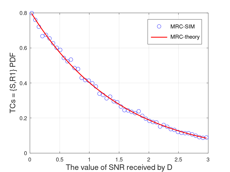
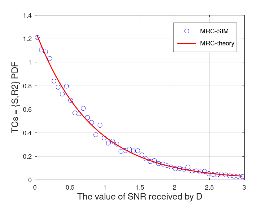
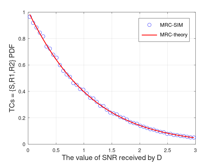
Figure 3: PDF of the value of SNR received by D in different TCs with parameters $\lambda_{1}=-12$ dB, $\lambda_{2}=-15$ dB, $R_{0}=2$ bit/s/Hz, $M_{1}=10$ mJoules, $M_{2}=8$ mJoules.

Fig. 4 and Fig. 5 depict the limiting PDF of energy stored in the R1 buffer and R2 buffer, obtained by simulation and theoretical analysis. It can be clearly seen from Fig. 4 that the solid line and dashed line almost exactly coincide, and they are almost in the middle of the simulation values. Furthermore, the same case can be seen in Fig. 5, which effectively proves the accuracy of the derived theoretical expressions in Eq. (66) and Eq. (57).

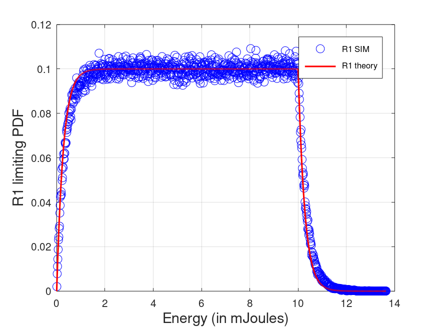
Figure 4: Limiting distribution of energy with infinite-size PEB of relay 1 and parameters $\lambda_{1}=-15$ dB, $\lambda_{2}=-12$ dB, $R_{0}=2$ bit/s/Hz, $M_{1}=10$ mJoules, $M_{2}=8$ mJoules.

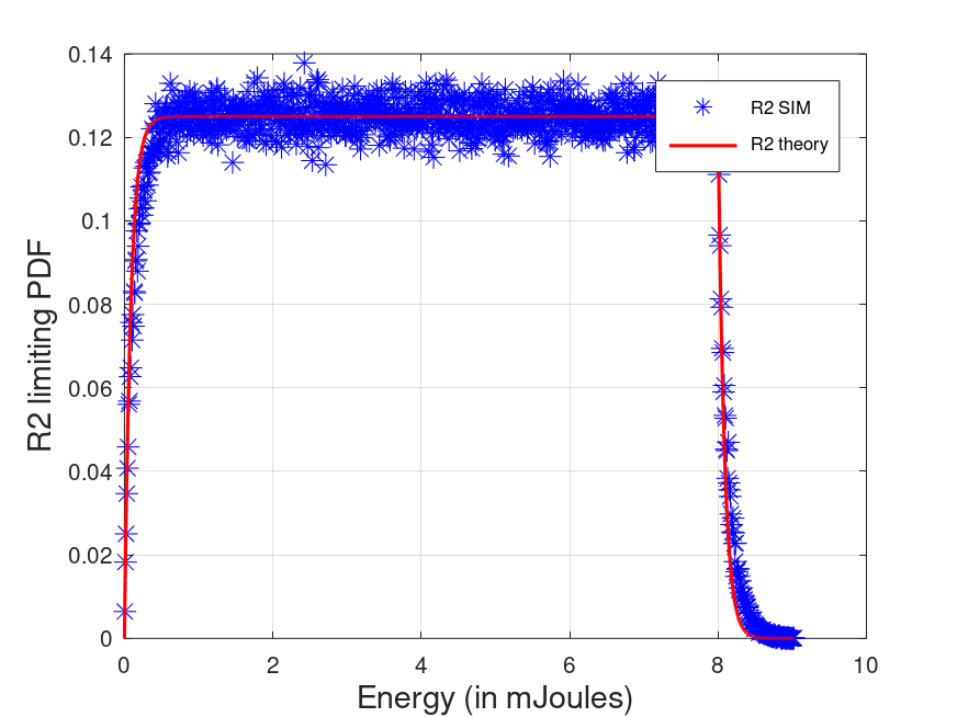
Figure 5: Limiting distribution of energy with finite-size PEB of relay 2 and parameters $\lambda_{1}=-15$ dB, $\lambda_{2}=-12$ dB, $R_{0}=2$ bit/s/Hz, $M_{1}=10$ mJoules, $M_{2}=8$ mJoules..

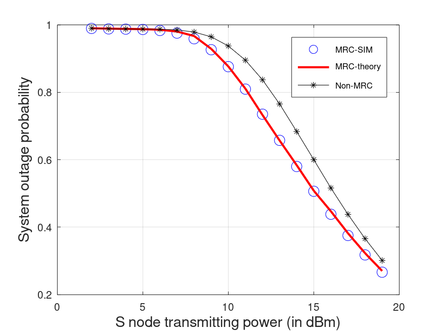
Figure 6: Outage probability of system vs. $P_{Ts}$, with parameters $\lambda_{1}=-11$ dB, $\lambda_{2}=-12$ dB, $R_{0}=2$ bit/s/Hz, $M_{1}=12$ mJoules, $M_{2}=10$ mJoules.

Fig. 6 shows the system outage probability of the system applied MRC obviously less than Non-MRC system. In additon, Fig. 7 depicts the throughput of system and our system also outperform to Non-MRC system. This is because the MRC algorithm can combine the multipath signal with the appropriate coefficient to achieve diversity gain. Furthermore, it can be obvserved that the outage and throughput change slightly, when $P_{Ts}$ is from 2 dBm to 8 dBm, and change considerably when $P_{Ts}$ is from 9 dBm to 19 dBm. The reason for this phenomenon is that, when $P_{Ts}$ is small, it is difficult for S node transmitting data packet reliably to any other node, in other words, in the whole system, only S node is activated in most time. With the increase in $P_{Ts}$, S node is able to transmit the data packet to relay nodes. With the help of relay nodes, the performance of system improves substantially.

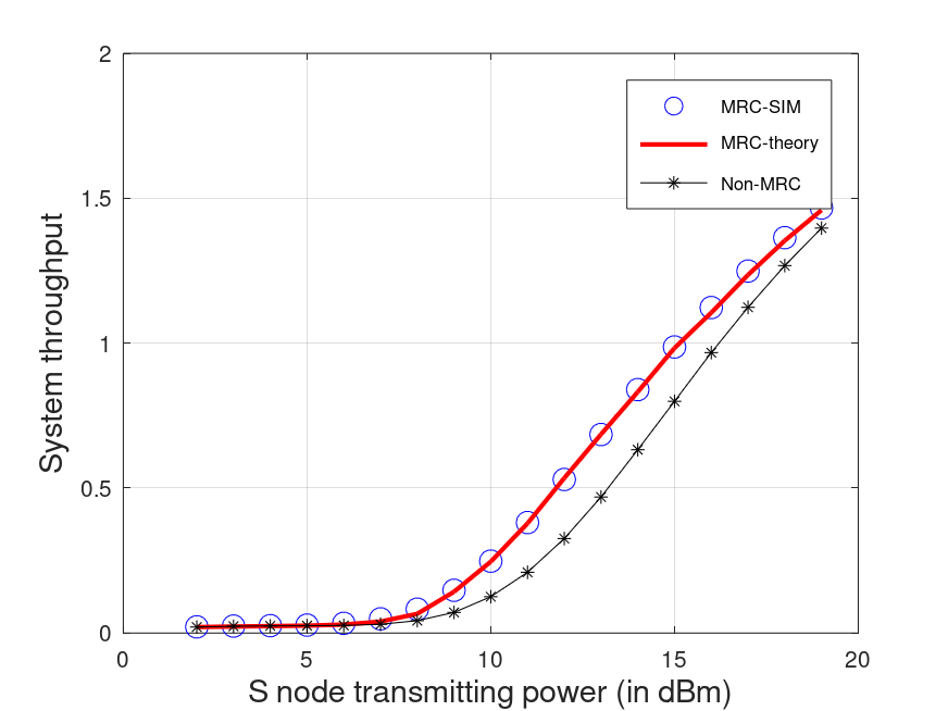
Figure 7: Throughput of system vs. $P_{Ts}$, with with parameters $\lambda_{1}=-11$ dB, $\lambda_{2}=-12$ dB, $R_{0}=2$ bit/s/Hz, $M_{1}=12$ mJoules, $M_{2}=10$ mJoules.

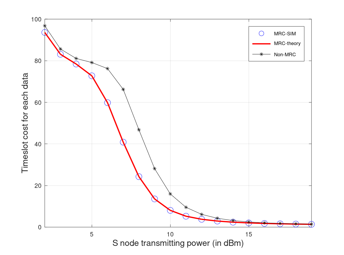
Figure 8: Timeslot cost for each data vs. $P_{Ts}$, with parameters $\lambda_{1}=-11$ dB, $\lambda_{2}=-12$ dB, $R_{0}=2$ bit/s/Hz, $M_{1}=12$ mJoules, $M_{2}=10$ mJoules.

In Fig. 8, the system timeslot cost for each data are demonstrated. These simulations can clarify that the MRC system outperforms the Non-MRC system. Furthermore, it can be seen that timeslot cost of MRC system is close to that of Non-MRC system when $P_{Ts}$ is from 2 dBm to 4 dBm and from 14 dBm to 19dBm. This is because, when $P_{Ts}$ is too small, the SNR of the signals combined is also too small to reach the SNR threshold and transmit the data packet. As a reasult, the effect of MRC is not obvious. And when $P_{Ts}$ is too large, even the Non-MRC system can transmit the data packet to D easily so that the effect of MRC is not significant. Thus, if $P_{Ts}$ is from 5 dBm to 13 dBm, the Non-MRC system is hard to utilize the SNR of single signal to reach SNR threshold, however, our MRC system can exploit the SNR of multiple signals combined to finish the data packet transmitting. Hence, in these cases, MRC significantly improves system performance.

VI Conclusion

This paper combines OR aided cooperative communication network with EH nodes and MRC. By applying the discrete-time continuous-state space Markov chain model, the theoretical algorithm-based expressions for limiting the distributions of stored energy in infinite-size buffers are derived. Furthermore, by using both the limiting distributions of energy buffers and data-broadcasted probability at nodes, the theoretical numerical expressions for outage probability and throughput of the network are obtained. In the future, combining the generalized selection combining (GSC) with OR under the assumption of an EH cooperative communication network is worth being studied.

Appendix A Algorithm for Probability $p_{s}$, $p_{SR1}$, $p_{SR2}$, $p_{1}$, $p_{2}$, $p_{3}$, $p_{\gamma_{overall1}}$, $p_{\gamma_{overall2}}$, $p_{\gamma_{overall3}}$, ’$\mathfrak{c}$’, ’$\mathfrak{d}$’, ’$\mathfrak{f}$’, ’$\mathfrak{g}$’, ’$\mathfrak{m}$’, ’$\mathfrak{n}$’ and ’$\mathfrak{o}$’ Based on STM

Specifically, in line 9, 26, 44 and 58, the judgment condition $(p(i)\leq 0\,|\,\textbf{T}(i)<0)$ indicates that there are non-positive elements in $\textbf{p}(i)$ or $\textbf{T}(i)$, which is not desirable, so the update process needs to be terminated. Moreover, in line 12, 29, 47 and 61, $(||\textbf{p}(i)-\textbf{p}(i+1)||_{2}<10^{-7})$ indicates that the update error is small enough and the update process has converged. Therefore, the update process can be terminated.

  Algorithm 1 probability $p_{s}$, $p_{SR1}$, $p_{SR2}$, $p_{1}$, $p_{2}$, $p_{3}$, $p_{\gamma_{overall1}}$, $p_{\gamma_{overall2}}$, $p_{\gamma_{overall3}}$, ’$\mathfrak{c}$’, ’$\mathfrak{d}$’, ’$\mathfrak{f}$’, ’$\mathfrak{g}$’, ’$\mathfrak{m}$’, ’$\mathfrak{n}$’ and ’$\mathfrak{o}$’ based on STM

 

1:$W_{SD}$, $W_{SR1}$, $W_{SR2}$, $W_{R1D}$, $W_{R1R2}$, $W_{R2D}$, $\Gamma_{th}$, $\lambda_{1}$, $\lambda_{2}$, $M_{R1}$, $M_{R2}$, $\mathcal{N}$.

2:Initialize $i_{4}=0$, $k_{4}=0$, $j_{1}$ and $j_{2}\in\{1,2,3,4,5,6\}$, $\textbf{p}(0)=[p_{s},p_{SR1},p_{SR2},p_{1},p_{2},p_{3}]=[\frac{1}{6},\frac{1}{6},\frac{1}{6},\frac{1}{6},\frac{1}{6},\frac{1}{6}]$, $PU1=PU2=\frac{1}{2}$.

3:while 1 do

4:     Calculate $\textbf{T1}(i_{4})$ and $\textbf{T2}(i_{4})$ according to equations from Eq. (36) to Eq. (39),

5:     $i_{1}=0$, $k_{1}=0$

6:     $\textbf{p}_{\gamma_{overall1}}(0)=[p_{\gamma_{overall1}}(1),...,p_{\gamma_{overall1}}(\mathcal{N})]$

7:     $p_{\gamma_{overall1}}(j)=\frac{1}{\mathcal{N}}$, $1\leq j\leq\mathcal{N}$ and $j\in Z$

8:     while 1 do

9:         $\textbf{p}_{\gamma_{overall1}}(i_{1}+1)=\textbf{p}_{\gamma_{overall1}}(i_{1})\textbf{T1}(i_{4})$,

10:         if $(\textbf{p}_{\gamma_{overall1}}(i)\leq 0\,|\ |\,\textbf{T1}(i_{4})<0)$ then

11:              $k_{1}=i_{1}-1$,

12:              break,

13:         else if $(||\textbf{p}_{\gamma_{overall1}}(i_{1})-\textbf{p}_{\gamma_{overall1}}(i_{1}+1)||_{2}<10^{-7})$ then

14:              $k_{1}=i_{1}$,

15:              break,

16:         else

17:              $i_{1}=i_{1}+1$,

18:         end if

19:     end while

20:     $p_{\gamma_{overall1}}=\textbf{p}_{\gamma_{overall1}}(k_{1})$

21:     

22:     $i_{2}=0$, $k_{2}=0$

23:     $\textbf{p}_{\gamma_{overall2}}(0)=[p_{\gamma_{overall2}}(1),...,p_{\gamma_{overall2}}(\mathcal{N})]$

24:     $p_{\gamma_{overall2}}(j)=\frac{1}{\mathcal{N}}$, $1\leq j\leq\mathcal{N}$ and $j\in Z$

25:     while 1 do

26:         $\textbf{p}_{\gamma_{overall2}}(i_{2}+1)=\textbf{p}_{\gamma_{overall2}}(i_{2})\textbf{T2}(i)$,

27:         if $(\textbf{p}_{\gamma_{overall2}}(i)\leq 0\,|\ |\,\textbf{T2}(i_{4})<0)$ then

28:              $k_{2}=i_{2}-1$,

29:              break,

30:         else if $(||\textbf{p}_{\gamma_{overall2}}(i_{2})-\textbf{p}_{\gamma_{overall2}}(i_{2}+1)||_{2}<10^{-7})$ then

31:              $k_{2}=i_{2}$,

32:              break,

33:         else

34:              $i_{2}=i_{2}+1$,

35:         end if

36:     end while

37:     $p_{\gamma_{overall2}}=\textbf{p}_{\gamma_{overall2}}(k_{2})$

38:     

39:     Calculate $\textbf{T3}(i_{4})$, $p_{d_{S->R2}}$ and $p_{d_{R1->R2}}$ according to equations from Eq. (40) to Eq. (45),

40:     $i_{3}=0$, $k_{3}=0$

41:     $\textbf{p}_{\gamma_{overall3}}(0)=[p_{\gamma_{overall3}}(1),...,p_{\gamma_{overall3}}(\mathcal{N})]$

42:     $p_{\gamma_{overall3}}(j)=\frac{1}{\mathcal{N}}$, $1\leq j\leq\mathcal{N}$ and $j\in Z$

43:     while 1 do

44:         $\textbf{p}_{\gamma_{overall3}}(i_{3}+1)=\textbf{p}_{\gamma_{overall3}}(i_{3})\textbf{T3}(i_{4})$,

45:         if $(\textbf{p}_{\gamma_{overall3}}(i)\leq 0\,|\ |\,\textbf{T3}(i_{4})<0)$ then

46:              $k_{3}=i_{3}-1$,

47:              break,

48:         else if $(||\textbf{p}_{\gamma_{overall3}}(i_{3})-\textbf{p}_{\gamma_{overall3}}(i_{3}+1)||_{2}<10^{-7})$ then

49:              $k_{3}=i_{3}$,

50:              break,

51:         else

52:              $i_{3}=i_{3}+1$,

53:         end if

54:     end while

55:     $p_{\gamma_{overall3}}=\textbf{p}_{\gamma_{overall3}}(k_{3})$

56:     Calculate ’$\mathfrak{c}$’, ’$\mathfrak{d}$’, ’$\mathfrak{f}$’, ’$\mathfrak{g}$’, ’$\mathfrak{m}$’, ’$\mathfrak{n}$’ and ’$\mathfrak{o}$’ and equations from Eq. (46) to Eq. (53),

57:     Calculate $\textbf{T}(i)$ according to $\textbf{p}(i)$ and equations from Eq. (20) to Eq. (35),

58:     $\textbf{p}(i_{4}+1)=\textbf{p}(i_{4})\textbf{T}(i_{4})$,

59:     if $(\textbf{p}_{j_{1}}(i)\leq 0\,|\ |\,\textbf{T}_{j_{1},j_{2}}(i_{4})<0)$ then

60:         $k_{4}=i_{4}-1$,

61:         break,

62:     else if $(||\textbf{p}(i_{4})-\textbf{p}(i_{4}+1)||_{2}<10^{-7})$ then

63:         $k_{=}i_{4}$,

64:         break,

65:     else

66:         $i_{4}=i_{4}+1$,

67:     end if

68:end while

69:Probability Distribution $\textbf{p}(k_{4})$, $p_{\gamma_{overall1}}$, $p_{\gamma_{overall2}}$, $p_{\gamma_{overall3}}$, ’$\mathfrak{c}$’, ’$\mathfrak{d}$’, ’$\mathfrak{f}$’, ’$\mathfrak{g}$’, ’$\mathfrak{m}$’, ’$\mathfrak{n}$’ and ’$\mathfrak{o}$’.

 

Appendix B Proof of Theorem 1

According to the total probability theorem, $\mathbb{P}_{21}$ and $\mathbb{P}_{22}$, the CDF of $B_{2}(i+1)$ in storage process in Eq. (54) may be evaluated as follows

$$\begin{split}&\mathrm{Pr}\{B_{2}(i+1)\leq x\}\\ &=\mathrm{Pr}\{B_{2}(i)+X(i)\leq x,TCs=\{S\}\}\\ &+\mathrm{Pr}\{B_{2}(i)+X(i)\leq x,TCs=\{S,R1\}\}\\ &+\mathrm{Pr}\{B_{2}(i)+X(i)\leq x,TCs=\{S,R2\},B_{2}(i)<M_{R2}\}\\ &+\mathrm{Pr}\{B_{2}(i)+X(i)\leq x,TCs=\{S,R2\},B_{2}(i)\geq M_{R2},\mathbb{M},\mathbb{N}\}\\ &+\mathrm{Pr}\{B_{2}(i)+X(i)\leq x,TCs=\{S,R2\},B_{2}(i)\geq M_{R2},\overline{\mathbb{C}}\}\\ &+\mathrm{Pr}\{B_{2}(i)+X(i)\leq x,TCs=\{S,R1,R2\},\\ &\qquad\qquad B_{2}(i)\geq M_{R2},\mathbb{O},\mathbb{F}\}\\ &+\mathrm{Pr}\{B_{2}(i)+X(i)\leq x,TCs=\{S,R1,R2\},\\ &\qquad\qquad B_{2}(i)\geq M_{R2},\overline{\mathbb{O}}\}\\ &+\mathrm{Pr}\{B_{2}(i)+X(i)\leq x,TCs=\{S,R1,R2\},B_{2}(i)<M_{R2}\}\\ &+\mathrm{Pr}\{B_{2}(i)-M_{R2}+X(i)\leq x,TCs=\{S,R2\},\\ &\qquad\qquad B_{2}(i)\geq M_{R2},\mathbb{M},\overline{\mathbb{N}}\}\\ &+\mathrm{Pr}\{B_{2}(i)-M_{R2}+X(i)\leq x,TCs=\{S,R1,R2\},\\ &\qquad\qquad B_{2}(i)\geq M_{R2},{\mathbb{O}},\overline{\mathbb{F}}\},\end{split}$$ (81)

When $i\to\infty$, the equation $\mathrm{Pr}\{B_{2}(i+1)\leq x\}=G^{i+1}_{2}(x)=G^{i}_{2}(x)=G_{2}(x)$ holds for the steady state of energy buffer at RNs. Thus, Eq. (81) can be written as follows

$$\begin{split}G_{2}(x)&=\left(p_{S}+p_{SR1}\right)\int_{\mu_{2}=0}^{x}F_{X}(x-\mu_{2})g_{2}(\mu_{2})\,d\mu_{2}\\ &+\big{(}p_{SR2}*(\mathfrak{m}*\mathfrak{n}+1-\mathfrak{m})\\ &+(p_{1}+p_{2}+p_{3})(\mathfrak{o}*\mathfrak{f}+1-\mathfrak{o})\big{)}\\ &\times\int_{\mu_{2}=M_{R2}}^{x}F_{X}(x-\mu_{2})g_{2}(\mu_{2})d\mu_{2}\\ &+(p_{SR2}+p_{SR1R2})\int_{\mu_{2}=0}^{min(x,M_{R2})}F_{X}(x-\mu_{2})g_{2}(\mu_{2})\,d\mu_{2}\\ &+\big{(}p_{SR2}*\mathfrak{m}*(1-\mathfrak{n})+(p_{1}+p_{2}+p_{3})*\mathfrak{o}*(1-\mathfrak{f})\big{)}\\ &\times\int_{\mu_{2}=M_{R2}}^{x+M_{R2}}F_{X}(x+M_{R2}-\mu_{2})g_{2}(\mu_{2})\,d\mu_{2},\end{split}$$ (82)

where $g_{2}(x)$ is the derivative of $G_{2}(x)$. With simplifying Eq. (82), we arrive at

$$G_{2}(x)=\begin{cases}G_{21}(x),&0\leq x<M_{R2}\\ G_{22}(x),&x\geq M_{R2}\end{cases}$$ (83)

where,

$$\begin{split}G_{21}(x)&=b_{2}\int_{\mu_{2}=M_{R2}}^{x+M_{R2}}F_{X}(x+M_{R2}-\mu_{2})g_{1}(\mu_{2})\,d\mu_{2}\\ &\quad+\int_{\mu_{2}=0}^{x}F_{X}(x-\mu_{2})g_{1}(\mu_{2})\,d\mu_{2},0\leq x<M_{R2}\end{split}$$ (84)

$$\begin{split}G_{22}(x)&=\int_{\mu_{2}=0}^{M_{R2}}F_{X}(x-\mu_{2})g_{2}(\mu_{2})\,d\mu_{2}\\ &\quad+a_{2}\int_{\mu_{2}=M_{R2}}^{x}F_{X}(x-\mu_{2})g_{2}(\mu_{2})\,d\mu_{2}\\ &\quad+b_{2}\int_{\mu_{2}=M_{R2}}^{x+M_{R2}}F_{X}(x+M_{R2}-\mu_{2})g_{2}(\mu_{2})\,d\mu_{2},\\ &\qquad\qquad\qquad\qquad\qquad\qquad\qquad\quad x\geq M_{R2}\end{split}$$ (85)

where,

$$\begin{split}a_{2}&=p_{S}+p_{SR1}+p_{SR2}*\mathfrak{m}*\mathfrak{n}\\ &+(p_{1}+p_{2}+p_{3})\big{(}\mathfrak{o}*\mathfrak{f}+(1-\mathfrak{o})\big{)}+P_{SR2}*(1-\mathfrak{m}),\end{split}$$ (86)

$$\begin{split}b_{2}&=p_{SR2}*\mathfrak{m}(1-\mathfrak{n})+(p_{1}+p_{2}+p_{3})*\mathfrak{o}(1-\mathfrak{f}).\end{split}$$ (87)

According to Eq. (83), the PDF $g_{2}(x)$ may be defined as

$$g_{2}(x)=\begin{cases}g_{21}(x),&0\leq x<M_{R2}\\ g_{22}(x),&x\geq M_{R2}.\end{cases}$$ (88)

Substituting Eq. (88) into Eq. (85), the derivatives about $x$ on both sides of Eq. (85) can be obtained as follows

$$\begin{split}g_{22}(x)&=\int_{\mu_{1}=0}^{M_{R2}}f_{X}(x-\mu_{2})g_{21}(\mu_{2})\,d\mu_{2}\\ &\quad+a_{2}\int_{\mu_{1}=M_{R2}}^{x}f_{X}(x-\mu_{2})g_{22}(\mu_{2})\,d\mu_{2}+b_{2}\\ &\quad\times\int_{\mu_{1}=M_{R2}}^{x+M_{R2}}f_{X}(x+M_{R2}-\mu_{2})g_{22}(\mu_{2})\,d\mu_{2},\\ &\qquad\qquad\qquad\qquad\qquad\qquad\qquad x\geq M_{R2}\end{split}$$ (89)

Obviously, $a_{2}+b_{2}=1$. In addtion,with [6], it is declared that, when $M_{R2}>\mathbb{E}[X(i)]=1/\lambda_{2}$, the energy update process in Eq. (54) possesses a unique stationary distribution, namely, $g_{2}(x)$ has unique solution. Furthermore, form [6], $g_{22}(x)$ can be assumed to have an exponential form solution, which can be expressed by $g_{22}(x)=k_{2}e^{Q_{2}x}$. Substituting $g_{22}(x)=k_{2}e^{Q_{2}x}$ and $f_{X}(x)=\lambda_{2}e^{-\lambda_{2}x}$ into Eq. (89), we obtain

$$\begin{split}k_{2}e^{Q_{2}x}&=\int_{\mu_{2}=0}^{M_{R2}}\lambda_{2}e^{-\lambda_{2}(x-\mu_{2})}g_{21}(\mu_{2})\,d\mu_{2}\\ &\quad+a_{2}\int_{\mu_{1}=M_{R2}}^{x}\lambda_{2}e^{-\lambda_{2}(x-\mu_{2})}k_{2}e^{Q_{2}\mu_{2}}\,d\mu_{2}+b_{2}\\ &\quad\times\int_{\mu_{1}=M_{R2}}^{x+M_{R2}}\lambda_{2}e^{-\lambda_{2}(x+M_{R2}-\mu_{2})}k_{2}e^{Q_{2}\mu_{2}}\,d\mu_{2},\\ &\qquad\qquad\qquad\qquad\qquad\qquad\qquad x\geq M_{R2}\end{split}$$ (90)

Simplifying Eq. (90), we obtain

$$\begin{split}k_{2}e^{Q_{2}x}&=\lambda_{2}e^{-\lambda_{2}x}\int_{\mu_{2}=0}^{M_{R2}}e^{\lambda_{2}\mu_{2}}g_{21}(\mu_{2})\,d\mu_{2}\\ &\quad-\dfrac{k_{2}\lambda_{2}e^{\left(Q_{2}M_{R2}-\lambda_{2}x\right)}\left(a_{2}e^{\lambda_{2}M_{R2}}+b_{2}\right)}{\lambda_{2}+Q_{2}}\\ &\quad+\dfrac{\lambda_{2}\left(a_{2}+b_{2}e^{Q_{2}M_{R2}}\right)k_{2}e^{Q_{2}x}}{\lambda_{2}+Q_{2}},x\geq M_{R2}\end{split}$$ (91)

For Eq. (91) to hold, the following conditions need to be satisfied

$$\dfrac{\lambda_{2}\left(a_{2}+b_{2}e^{Q_{2}M_{R2}}\right)}{\lambda_{2}+Q_{2}}=1,$$ (92a)

$$\dfrac{k_{2}e^{Q_{2}M_{R2}}\left(a_{2}e^{\lambda_{2}M_{R2}}+b_{2}\right)}{\lambda_{2}+Q_{2}}=\int_{\mu_{2}=0}^{M_{R2}}e^{\lambda_{2}\mu_{2}}g_{21}(\mu_{2})\,d\mu_{2}.$$ (92b)

The desirable solution $Q_{2}$ of Eq. (92a) for the finite distribution of $g_{22}(x)$ may be obtained by simplifying Eq. (92a) as follows

$$b_{2}\lambda_{2}e^{Q_{2}M_{R2}}=\lambda_{2}-a_{2}\lambda_{2}+Q_{2}=b_{2}\lambda_{2}+Q_{2},$$ (93)

Although, it can be easily found from Eq. (92a) that $Q_{2_{0}}=0$ is one of the solutions of $Q_{2}$ in Eq. (92a), $Q_{2_{0}}$ does not satisfy the condition that $g_{22}(x)$ is a limiting distribution. And the other solution $Q_{2_{1}}$ of $Q_{2}$ in Eq. (92a) can be obtained by simplifying Eq. (92a) as

$$Q_{2}=\frac{-W\left(-b_{2}\lambda_{2}M_{R2}e^{-b_{2}\lambda_{2}M_{R2}}\right)}{M_{R2}}-b_{2}\lambda_{2},\quad b_{2}\lambda_{2}M_{R2}>1.$$ (94)

where, with $b_{2}\lambda_{2}M_{R2}>1$, $W\left(-b_{2}\lambda_{2}M_{R2}e^{-b_{2}\lambda_{2}M_{R2}}\right)>-b_{2}\lambda_{2}M_{R2}$ so that $Q_{2}<0$, ensuring the finite distribution of $g_{22}(x)$.

Correspondingly, when $0\leq x<M_{R2}$, substitute Eq. (88) into Eq. (84) and differentiate both sides of Eq. (84) with respect to $x$. we have

$$\begin{split}g_{21}(x)&=b_{2}\int_{\mu_{2}=M_{R2}}^{x+M_{R2}}f_{X}(x+M_{R2}-\mu_{2})g_{22}(\mu_{2})\,d\mu_{2}\\ &\quad+\int_{\mu_{2}=0}^{x}f_{X}(x-\mu_{2})g_{21}(\mu_{2})\,d\mu_{2},0\leq x<M_{R2}\end{split}$$ (95)

Substituting $g_{22}(x)=k_{2}e^{Q_{2}x}$ and $f_{X}(x)=\lambda_{2}e^{-\lambda_{2}x}$ into Eq. (95), we get

$$\begin{split}g_{21}(x)&=\lambda_{2}\int_{\mu_{2}=0}^{x}e^{-\lambda_{2}\left(x-\mu_{2}\right)}g_{21}(\mu_{2})\,d\mu_{2}\\ &\quad+\dfrac{b_{2}k_{2}\lambda_{2}e^{Q_{2}M_{R2}}}{\lambda_{2}+Q_{2}}\left(e^{Q_{2}x}-e^{-\lambda_{2}x}\right),0\leq x<M_{R2}\end{split}$$ (96)

Let $r(x)=\frac{b_{2}k_{2}\lambda_{2}e^{Q_{2}M_{R2}}}{\lambda_{2}+Q_{2}}\left(e^{Q_{2}x}-e^{-\lambda_{2}x}\right)$, and the integral equation in Eq. (96) can be rewritten as follows

$$\begin{split}g_{21}(x)=\lambda_{2}\int_{\mu_{2}=0}^{x}e^{-\lambda_{2}\left(x-\mu_{2}\right)}g_{21}(\mu_{2})\,d\mu_{2}+r(x),0\leq x<M_{R2}\end{split}$$ (97)

Clearly, Eq. (97) is a Volterra integral equation of the second kind, whose solution is given by [6], [7] and [21, eq. 2.2.1]

$$\begin{split}g_{21}(x)=r(x)+\lambda_{2}\int_{t=0}^{x}r(t)\,dt,\end{split}$$ (98)

Substituting $r(x)$ into Eq. (98), we obtain

$$\begin{split}g_{21}(x)&=\dfrac{b_{2}k_{2}\lambda_{2}e^{Q_{2}M_{R2}}}{\lambda_{2}+Q_{2}}\left(e^{Q_{2}x}-e^{-\lambda_{2}x}\right)\\ &\quad+\lambda_{2}\int_{t=0}^{x}\dfrac{b_{2}k_{2}\lambda_{2}e^{Q_{2}M_{R2}}}{\lambda_{2}+Q_{2}}\left(e^{Q_{2}t}-e^{-\lambda_{2}t}\right)\,dt\\ &=\dfrac{b_{2}k_{2}\lambda_{2}e^{Q_{2}M_{R2}}\left(e^{Q_{2}x}-1\right)}{Q_{2}},0\leq x<M_{R2}\end{split}$$ (99)

Because of the unit area condition on $g_{2}(x)$, we have

$$\int_{x=0}^{\infty}g_{2}(x)\,dx=\int_{x=0}^{M_{R2}}g_{21}(x)\,dx+\int_{x=M_{R2}}^{\infty}g_{22}(x)\,dx=1,$$ (100)

Substituting $g_{21}(x)=\frac{b_{2}k_{2}\lambda_{2}e^{Q_{2}M_{R2}}\left(e^{Q_{2}x}-1\right)}{Q_{2}}$ and $g_{22}(x)=k_{2}e^{Q_{2}x}$ into Eq. (100), we arrive at

$$k_{2}=\dfrac{-Q_{2}}{M_{R2}\left(b_{2}\lambda_{2}+Q_{2}\right)},$$ (101)

Furthermore, according to Eq. (101), we have

$$g_{21}(x)=\dfrac{1-e^{Q_{2}x}}{M_{R2}}.$$ (102)

Substituting Eq. (102) into the right side of Eq. (92b), we obtain

$$\begin{split}\int_{\mu_{2}=0}^{M_{R2}}e^{\lambda_{2}\mu_{2}}g_{21}(\mu_{2})\,d\mu_{2}&=\int_{\mu_{2}=0}^{M_{R2}}\dfrac{\left(1-e^{Q_{2}x}\right)e^{\lambda_{2}\mu_{2}}}{M_{R2}}\,d\mu_{2}\\ &=\dfrac{1-e^{\left(\lambda_{2}+Q_{2}\right)M_{R2}}}{\left(\lambda_{2}+Q_{2}\right)M_{R2}}-\dfrac{1-e^{\lambda_{2}M_{R2}}}{\lambda_{2}M_{R2}},\end{split}$$ (103)

The equation in Eq. (92a) leads us to conclude $\lambda_{2}M_{R2}=\frac{\left(\lambda_{2}+Q_{2}\right)M_{R2}}{b_{2}e^{Q_{2}M_{R2}}+a_{2}}$. Substituting this conclusion in Eq. (103), we have

$$\begin{split}\int_{\mu_{2}=0}^{M_{R2}}e^{\lambda_{2}\mu_{2}}g_{21}(\mu_{2})\,d\mu_{2}=\dfrac{\left(1-e^{Q_{2}M_{R2}}\right)\left(b_{2}+a_{2}e^{\lambda_{2}M_{R2}}\right)}{\left(\lambda_{2}+Q_{2}\right)M_{R2}},\end{split}$$ (104)

Similarly, the conclude $1-e^{Q_{2}M_{R2}}=\frac{-Q_{2}}{b_{2}\lambda_{2}}$ may be obtained from Eq. (93). Substituting this conclusion in Eq. (104), we arrive at

$$\begin{split}\int_{\mu_{2}=0}^{M_{R2}}e^{\lambda_{2}\mu_{2}}g_{21}(\mu_{2})\,d\mu_{2}&=\dfrac{\left(1-e^{Q_{2}M_{R2}}\right)\left(b_{2}+a_{2}e^{\lambda_{2}M_{R2}}\right)}{\left(\lambda_{2}+Q_{2}\right)M_{R2}}\\ &=\dfrac{-Q_{2}\left(b_{2}+a_{2}e^{\lambda_{2}M_{R2}}\right)}{\left(\lambda_{2}+Q_{2}\right)M_{R2}b_{2}\lambda_{2}}\\ &=\dfrac{-Q_{2}e^{Q_{2}M_{R2}}\left(b_{2}+a_{2}e^{\lambda_{2}M_{R2}}\right)}{M_{R2}\left(b_{2}\lambda_{2}+Q_{2}\right)\left(\lambda_{2}+Q_{2}\right)}\\ &=\dfrac{k_{2}e^{Q_{2}M_{R2}}\left(b_{2}+a_{2}e^{\lambda_{2}M_{R2}}\right)}{\lambda_{2}+Q_{2}}.\end{split}$$ (105)

Now, the validation of Eq. (92b) in Eq. (105) indicates that the unique solution $g_{21}(x)$ in Eq. (102) for Eq. (95) and the unique solution $g_{22}(x)=k_{2}e^{Q_{2}x}$ for Eq. (89) are obtained.

Appendix C Proof of Theorem 2

According to the energy storage process $B_{2}(i)$ with the infinite-size energy buffer in Eq. (61), the variable $O_{R}(i)$ is defined by

$$O_{R}(i)=\begin{cases}1,\quad\mathbb{P}_{I1}\\ 0,\quad\mathbb{P}_{II1}\end{cases}$$ (106)

where $\mathbb{P}_{I1}$ and $\mathbb{P}_{II1}$ are the conditions required for the equations in Eq. (106) to hold. Specifically, they can be expressed as follows

$$\begin{split}\mathbb{P}_{I1}:\,&\Big{[}\big{(}TCs=\{S,R2\}\big{)}\cap\mathbb{C}\cap\overline{\mathbb{N}}\Big{]}\\ &\cup\Big{[}\big{(}TCs=\{S,R1,R2\}\big{)}\cap\mathbb{O}\cap\overline{\mathbb{F}}\Big{]},\end{split}$$ (107)

$$\begin{split}\mathbb{P}_{II1}:\,&\big{(}TCs=\{S\}\big{)}\cup\big{(}TCs=\{S,R1\}\big{)}\\ &\cup\Big{[}\big{(}TCs=\{S,R2\}\big{)}\cap\mathbb{C}\cap\mathbb{N}\Big{]}\\ &\cup\Big{[}\big{(}TCs=\{S,R2\}\big{)}\cap\overline{\mathbb{C}}\Big{]}\\ &\cup\Big{[}\big{(}TCs=\{S,R1,R2\}\big{)}\cap\mathbb{O}\cap\mathbb{F}\Big{]}\\ &\cup\Big{[}\big{(}TCs=\{S,R1,R2\}\big{)}\cap\overline{\mathbb{O}}\Big{]}.\end{split}$$ (108)

Moreover, the variable $\theta(i)$ is defined as follows

$$\theta(i)=\begin{cases}1,\quad B_{2}(i)\geq M_{R2}\\ 0,\quad B_{2}(i)<M_{R2}\end{cases}$$ (109)

Implying Eq. (106), Eq. (107),Eq. (108) and Eq. (109), the energy storage process in Eq. (61) can be re-expressed as follows

$$B_{2}(i+1)-B_{2}(i)=X(i)-M_{R2}\theta(i)O_{R}(i).$$ (110)

According to the law of large numbers, the average energy harvesting rate can be obtained as follows

$$\mathbb{E}[X(i)]=\lim_{N\to\infty}\frac{1}{N}\sum_{i=1}^{N}X(i),$$ (111)

Similarly, the average energy consumption rate can be given by

$$\begin{split}\mathbb{E}[M_{R2}\theta(i)O_{R}(i)]&=\lim_{N\to\infty}\frac{1}{N}\sum_{i=1}^{N}M_{R2}\theta(i)O_{R}(i)\\ &=\lim_{N\to\infty}\frac{1}{N}\sum_{B_{2}(i)\geq M_{R2}}M_{R2}O_{R}(i)\\ &\leq M_{R2}\Big{\{}\lim_{N\to\infty}\frac{1}{N}\sum_{i=1}^{N}O_{R}(i)\Big{\}},\end{split}$$ (112)

And,

$$\begin{split}\mathbb{E}[O_{R}(i)]&=\lim_{N\to\infty}\frac{1}{N}\sum_{i=1}^{N}O_{R}(i)\\ &=1\times\mathrm{Pr}\{O_{R}(i)=1\}+0\times\mathrm{Pr}\{O_{R}(i)=0\}\\ &=\mathrm{Pr}\{B_{2}(i)-M_{R2}+X(i)\leq x,TCs=\{S,R2\},\\ &\qquad\qquad B_{2}(i)\geq M_{R2},\mathbb{M},\overline{\mathbb{N}}\}\\ &+\mathrm{Pr}\{B_{2}(i)-M_{R2}+X(i)\leq x,TCs=\{S,R1,R2\},\\ &\qquad\qquad B_{2}(i)\geq M_{R2},\mathbb{O},\overline{\mathbb{F}}\}\\ &=b_{2},\end{split}$$ (113)

From Eq. (112) and Eq. (113), we obtain

$$\begin{split}\mathbb{E}[M_{R2}\theta(i)O_{R}(i)]&\leq b_{1}.\end{split}$$ (114)

If $\psi_{R2}\leq 1$, from Eq. (57), we get

$$\begin{split}\mathbb{E}[X(i)]&\geq M_{R2}b_{2},\end{split}$$ (115)

Therefore, if $\psi_{1}\leq 1$, from Eq. (111), Eq. (112), Eq. (114) and Eq. (115), we obtain

$$\lim_{N\to\infty}\frac{1}{N}\sum_{i=1}^{N}X(i)\geq\lim_{N\to\infty}\frac{1}{N}\sum_{i=1}^{N}M_{R2}\theta(i)O_{R}(i),$$ (116)

According to Eq. (110) and Eq. (116), we have

$$\lim_{N\to\infty}\frac{1}{N}\sum_{i=1}^{N}B_{2}(i+1)\geq\lim_{N\to\infty}\frac{1}{N}\sum_{i=1}^{N}B_{2}(i),$$ (117)

Clearly, if the inequality condition holds in Eq. (117), the comparison of between $B_{1}(i+1)$ and $B_{1}(i)$ shows that the energy accumulates in the buffer over time slot, i.e., $\begin{matrix}\lim_{i\to\infty}\mathbb{E}[B_{1}(i)]=\infty\end{matrix}$. Therefore, the stationary distribution of $B_{1}(i)$ does not exist, and after a finite number of time slots, $B_{1}(i)>M_{R1}$ almost always hold. In addition, if the equality condition holds in Eq. (116), according to Eq. (116) and Eq. (112), we get

$$\lim_{N\to\infty}\frac{1}{N}\sum_{i=1}^{N}X(i)=\lim_{N\to\infty}\frac{1}{N}\sum_{B_{2}(i)\geq M_{R2}}M_{R2}O_{R}(i).$$ (118)

Eq. (118) indicates that in the energy buffer with DCSMC model, the average energy harvesting rate equals the average energy consumption rate, which is unstable [22]. Therefore, the buffer may almost always provide $M_{R2}$ amount of energy.

Appendix D Proof of Theorem 3

On the basis of the total probability theorem, $\mathbb{P}_{11}$ and $\mathbb{P}_{12}$ form a complete set of events accompanying event $B_{1}(i+1)$. Thus, the cumulative distribution function (CDF) of $B_{1}(i+1)$ in the energy update process in Eq. (61) can be expressed as follows

$$\begin{split}&\mathrm{Pr}\{B_{1}(i+1)\leq x\}\\ &=\mathrm{Pr}\{B_{1}(i)+X(i)\leq x,TCs=\{S\}\}\\ &+\mathrm{Pr}\{B_{1}(i)+X(i)\leq x,TCs=\{S,R2\}\}\\ &+\mathrm{Pr}\{B_{1}(i)+X(i)\leq x,\big{(}TCs=\{S,R1\}\big{)},\big{(}B_{1}(i)<M_{R1}\big{)}\}\\ &+\mathrm{Pr}\{B_{1}(i)+X(i)\leq x,\big{(}TCs=\{S,R1\}\big{)},\big{(}B_{1}(i)\geq M_{R1},\\ &\qquad\mathbb{C},\mathbb{D},\gamma_{SR2}(i)\geq\Gamma_{th},\big{)}\}\\ &+\mathrm{Pr}\{B_{1}(i)+X(i)\leq x,\big{(}TCs=\{S,R1\}\big{)},\big{(}B_{1}(i)\geq M_{R1},\\ &\qquad\mathbb{C},\mathbb{D},\gamma_{SR2}(i)<\Gamma_{th},\gamma_{R1R2}(i)<\Gamma_{th}\big{)}\}\\ &+\mathrm{Pr}\{B_{1}(i)+X(i)\leq x,\big{(}TCs=\{S,R1,R2\}\big{)},\\ &\qquad\big{(}B_{2}(i)\geq M_{R2},\mathbb{O},\overline{\mathbb{F}}\big{)}\}\\ &+\mathrm{Pr}\{B_{1}(i)+X(i)\leq x,\big{(}TCs=\{S,R1,R2\}\big{)},\\ &\qquad\big{(}B_{2}(i)\geq M_{R2},\mathbb{O},\mathbb{F},B_{1}(i)\geq M_{R1},\mathbb{G}\big{)}\}\\ &+\mathrm{Pr}\{B_{1}(i)+X(i)\leq x,\big{(}TCs=\{S,R1,R2\}\big{)},\\ &\qquad\big{(}B_{2}(i)\geq M_{R2},\mathbb{O},\mathbb{F},B_{1}(i)<M_{R1}\big{)}\}\\ &+\mathrm{Pr}\{B_{1}(i)-M_{R1}+X(i)\leq x,\\ &\qquad\big{(}TCs=\{S,R1\}\big{)},\big{(}B_{1}(i)\geq M_{R1}\big{)},\mathbb{C},\overline{\mathbb{D}}\}\\ &+\mathrm{Pr}\{B_{1}(i)-M_{R1}+X(i)\leq x,\\ &\qquad\big{(}TCs=\{S,R1\}\big{)},\big{(}\big{(}B_{1}(i)\geq M_{R1}\big{)},\mathbb{C},\mathbb{D},\\ &\qquad\gamma_{SR2}(i)<\Gamma_{th},\gamma_{R1R2}(i)\geq\Gamma_{th}\big{)}\\ &+\mathrm{Pr}\{B_{1}(i)-M_{R1}+X(i)\leq x,\big{(}TCs=\{S,R1,R2\}\big{)},\\ &\qquad\big{(}B_{2}(i)\geq M_{R2},\mathbb{O},\mathbb{F},\big{(}B_{1}(i)\geq M_{R1}\big{)},\overline{\mathbb{G}}\big{)}\}\\ &+\mathrm{Pr}\{B_{1}(i)-M_{R1}+X(i)\leq x,\big{(}TCs=\{S,R1,R2\}\big{)},\\ &\qquad\big{(}B_{2}(i)<M_{R2},\mathbb{O},\big{(}B_{1}(i)\geq M_{R1}\big{)},\overline{\mathbb{G}}\big{)}\}.\end{split}$$ (119)

Let $\mathrm{Pr}\{B_{1}(i+1)\leq x\}=G^{i+1}_{1}(x)$. With $i\to\infty$, if the energy buffer is in its steady state, it obeys that, $\mathrm{Pr}\{B_{1}(i+1)\leq x\}=G^{i+1}_{1}(x)=G^{i}_{1}(x)=G_{1}(x)$. In this scenario, Eq. (119) can be written as follows

$$\begin{split}G_{1}(x)&=\Big{[}p_{S}+p_{SR2}+((p_{1}+p_{2}+p_{3})*o(1-f))PU2\\ &+(p_{1}+p_{2}+p_{3})(1-h)\Big{]}\int_{\mu_{1}=0}^{x}F_{X}(x-\mu_{1})g_{1}(\mu_{1})\,d\mu_{1}\\ &+\Big{[}p_{SR1}[\mathfrak{c}*\mathfrak{d}(\mathrm{Pr}\{\gamma_{SR2}(i)\geq\Gamma_{th}\}\\ &+\mathrm{Pr}\{\gamma_{SR2}(i)<\Gamma_{th}\}\mathrm{Pr}\{\gamma_{R1R2}(i)<\Gamma_{th}\})+1-\mathfrak{c}]\\ &+((p_{1}+p_{2}+p_{3})*\mathfrak{o}*\mathfrak{f}*\mathfrak{g})PU2\\ &+((p_{1}+p_{2}+p_{3})*\mathfrak{o}*\mathfrak{g})(1-PU2)\Big{]}\\ &\times\int_{\mu_{1}=M_{R1}}^{x}F_{X}(x-\mu_{1})g_{1}(\mu_{1})d\mu_{1}\\ &+\Big{[}p_{SR1}+PU2((p_{1}+p_{2}+p_{3})*\mathfrak{o}*\mathfrak{f})\\ &+(1-PU2)((p_{1}+p_{2}+p_{3})*\mathfrak{o})\Big{]}\\ &\times\int_{\mu_{1}=0}^{min(x,M_{R1})}F_{X}(x-\mu_{1})g_{1}(\mu_{1})\,d\mu_{1}\\ &+\Big{[}p_{SR1}*\mathfrak{c}((1-\mathfrak{d})+\mathfrak{d}(1-e^{-W_{SR2}\Gamma_{th}})e^{-W_{R1R2}\Gamma_{th}})\\ &+PU2((p_{1}+p_{2}+p_{3})*\mathfrak{o}*\mathfrak{f}(1-\mathfrak{g}))\\ &+(1-PU1)((p_{1}+p_{2}+p_{3})*\mathfrak{o}(1-\mathfrak{g})\Big{]}\\ &\times\int_{\mu_{1}=M_{R1}}^{x+M_{R1}}F_{X}(x+M_{R1}-\mu_{1})d\mu_{1},\end{split}$$ (120)

where $g_{1}(x)$ is the PDF of $B_{1}(i)$.$F_{X}(x)=1-e^{-\lambda_{1}x}$ is the CDF of $X$. By simplifying Eq. (120), we arrive at

$$G_{1}(x)=\begin{cases}G_{11}(x),&0\leq x<M_{R1}\\ G_{12}(x),&x\geq M_{R1}\end{cases}$$ (121)

where,

$$\begin{split}G_{11}(x)&=\int_{\mu_{1}=0}^{x}F_{X}(x-\mu_{1})g_{1}(\mu_{1})\,d\mu_{1}\\ &\quad+b_{1}\int_{\mu_{1}=M_{R1}}^{x+M_{R1}}F_{X}(x+M_{R1}-\mu_{1})g_{1}(\mu_{1})\,d\mu_{1},\\ &\qquad\qquad\qquad\qquad\qquad\qquad\qquad 0\leq x<M_{R1}\end{split}$$ (122)

$$\begin{split}G_{12}(x)&=\int_{\mu_{1}=0}^{M_{R1}}F_{X}(x-\mu_{1})g_{1}(\mu_{1})\,d\mu_{1}\\ &\quad+a_{1}\int_{\mu_{1}=M_{R1}}^{x}F_{X}(x-\mu_{1})g_{1}(\mu_{1})\,d\mu_{1}\\ &\quad+b_{1}\int_{\mu_{1}=M_{R1}}^{x+M_{R1}}F_{X}(x+M_{R1}-\mu_{1})g_{1}(\mu_{1})\,d\mu_{1},\\ &\qquad\qquad\qquad\qquad\qquad\qquad\qquad\quad x\geq M_{R1}\end{split}$$ (123)

where,

$$\begin{split}a_{1}&=p_{S}+p_{SR2}+((p_{1}+p_{2}+p_{3})*\mathfrak{o}(1-\mathfrak{f}))*PU2\\ &+(p_{1}+p_{2}+p_{3})(1-e)+p_{SR1}(\mathfrak{c}*\mathfrak{d}(e^{-W_{SR2}\Gamma_{th}}\\ &+(1-e^{-W_{SR2}\Gamma_{th}})(1-e^{-W_{R1R2}\Gamma_{th}}))\\ &+(1-\mathfrak{c}))+((p_{1}+p_{2}+p_{3})*\mathfrak{o}*\mathfrak{f}*\mathfrak{g})PU2\\ &+((p_{1}+p_{2}+p_{3})*\mathfrak{o}*\mathfrak{g})(1-PU2),\end{split}$$ (124)

$$\begin{split}b_{1}&=p_{SR1}*\mathfrak{c}((1-\mathfrak{d})+\mathfrak{d}(1-e^{-W_{SR2}\Gamma_{th}})e^{-W_{R1R2}\Gamma_{th}}\\ &+PU2((p_{1}+p_{2}+p_{3})*\mathfrak{o}*\mathfrak{f}(1-\mathfrak{g})\\ &+(1-PU2)*((p_{1}+p_{2}+p_{3})*\mathfrak{o}(1-\mathfrak{g})).\end{split}$$ (125)

According to Eq. (121), the PDF $g_{1}(x)$ may be defined as

$$g_{1}(x)=\begin{cases}g_{11}(x),&0\leq x<M_{R1}\\ g_{12}(x),&x\geq M_{R1}.\end{cases}$$ (126)

After substituting Eq. (126) into Eq. (123), the derivatives of Eq. (123) about $x$ can be obtained

$$\begin{split}g_{12}(x)&=\int_{\mu_{1}=0}^{M_{R1}}f_{X}(x-\mu_{1})g_{11}(\mu_{1})\,d\mu_{1}\\ &\quad+a_{1}\int_{\mu_{1}=M_{R1}}^{x}f_{X}(x-\mu_{1})g_{12}(\mu_{1})\,d\mu_{1}\\ &\quad+b_{1}\int_{\mu_{1}=M_{R1}}^{x+M_{R1}}f_{X}(x+M_{R1}-\mu_{1})g_{12}(\mu_{1})\,d\mu_{1},\\ &\qquad\qquad\qquad\qquad\qquad\qquad\qquad\quad x\geq M_{R1},\end{split}$$ (127)

Like $g_{22}(x)$ in appendix B, let $g_{12}(x)=k_{1}e^{Q_{1}x}$. Substituting $g_{12}(x)=k_{1}e^{Q_{1}x}$ and $f_{X}(x)=\lambda_{1}e^{-\lambda_{1}x}$ into Eq. (127), we get

$$\begin{split}k_{1}e^{Q_{1}x}&=\int_{\mu_{1}=0}^{M_{R1}}\lambda_{1}e^{-\lambda_{1}(x-\mu_{1})}g_{11}(\mu_{1})\,d\mu_{1}\\ &\quad+\left(1-b_{1}\right)\int_{\mu_{1}=M_{R1}}^{x}\lambda_{1}e^{-\lambda_{1}(x-\mu_{1})}k_{1}e^{Q_{1}\mu_{1}}\,d\mu_{1}+b_{1}\\ &\quad\times\int_{\mu_{1}=M_{R1}}^{x+M_{R1}}\lambda_{1}e^{-\lambda_{1}(x+M_{R1}-\mu_{1})}k_{1}e^{Q_{1}\mu_{1}}\,d\mu_{1},x\geq M_{R1}\end{split}$$ (128)

Simplifying Eq. (128), we have

$$\begin{split}k_{1}e^{Q_{1}x}&=\lambda_{1}e^{-\lambda_{1}x}\int_{\mu_{1}=0}^{M_{R1}}e^{\lambda_{1}\mu_{1}}g_{11}(\mu_{1})\,d\mu_{1}\\ &\quad-\dfrac{\lambda_{1}k_{1}\left[b_{1}+\left(1-b_{1}\right)e^{\lambda_{1}M_{R1}}\right]}{\lambda_{1}+Q_{1}}e^{\left(Q_{1}M_{R1}-\lambda_{1}x\right)}\\ &\quad+\dfrac{b_{1}\lambda_{1}e^{Q_{1}M_{R1}}+\left(1-b_{1}\right)\lambda_{1}}{\lambda_{1}+Q_{1}}k_{1}e^{Q_{1}x},x\geq M_{R1}\end{split}$$ (129)

In order to ensure $g_{12}(x)=k_{1}e^{Q_{1}x}$, the coefficients of corresponding terms in Eq. (129) both sides are equal. Thus, we get

$$\dfrac{b_{1}\lambda_{1}e^{Q_{1}M_{R1}}+a_{1}\lambda_{1}}{\lambda_{1}+Q_{1}}=1,$$ (130a)

$$\begin{aligned} &\dfrac{k_{1}e^{Q_{1}M_{R1}}\left[b_{1}+a_{1}e^{\lambda_{1}M_{R1}}\right]}{\lambda_{1}+Q_{1}}\\ &\qquad\qquad=\int_{\mu_{1}=0}^{M_{R1}}e^{\lambda_{1}\mu_{1}}g_{11}(\mu_{1})\,d\mu_{1}.\end{aligned}$$ (130b)

Although, it can be easily found from Eq. (130a) that $Q_{1_{0}}=0$ is one of the solutions of $Q_{1}$ in Eq. (130a), $Q_{1_{0}}$ does not satisfy the condition that $g_{12}(x)$ is a limiting distribution. And the other solution $Q_{1_{1}}$ of $Q_{1}$ in Eq. (130a) can be obtained by simplifying Eq. (130a) as

$$b_{1}\lambda_{1}e^{Q_{1}M_{R1}}=\lambda_{1}-a_{1}\lambda_{1}+Q_{1}=b_{1}\lambda_{1}+Q_{1},$$ (131)

With Lambert W function, the solution $Q_{1_{1}}$ can be expressed as follows

$$Q_{1}=\frac{-W\left(-b_{1}\lambda_{1}M_{R1}e^{-b_{1}\lambda_{1}M_{R1}}\right)}{M_{R1}}-b_{1}\lambda_{1},$$ (132)

Due to the property of Lambert W function, when $b_{1}\lambda_{1}M_{R1}\leq 1$, $W\left(-b_{1}\lambda_{1}M_{R1}e^{-b_{1}\lambda_{1}M_{R1}}\right)=-b_{1}\lambda_{1}M_{R1}$, as a result, $Q_{1_{1}}=Q_{1_{0}}=0$. On the other hand, when $b_{1}\lambda_{1}M_{R1}>1$, $W\left(-b_{1}\lambda_{1}M_{R1}e^{-b_{1}\lambda_{1}M_{R1}}\right)>-b_{1}\lambda_{1}M_{R1}$ so that $Q_{1_{1}}<0$, ensuring the limiting distribution of $g_{12}(x)$. Thus, for the stationary distribution of $g_{12}(x)$, we obtain

$$Q_{1}=\frac{-W\left(-b_{1}\lambda_{1}M_{R1}e^{-b_{1}\lambda_{1}M_{R1}}\right)}{M_{R1}}-b_{1}\lambda_{1},\quad b_{1}\lambda_{1}M_{R1}>1.$$ (133)

Similarly, when $0\leq x<M_{R1}$, substituting Eq. (126) into Eq. (122), the derivatives of Eq. (122) about $x$ can be obtained

$$\begin{split}g_{11}(x)&=b_{1}\int_{\mu_{1}=M_{R1}}^{x+M_{R1}}f_{X}(x+M_{R1}-\mu_{1})g_{12}(\mu_{1})\,d\mu_{1}\\ &\quad+\int_{\mu_{1}=0}^{x}f_{X}(x-\mu_{1})g_{11}(\mu_{1})\,d\mu_{1},0\leq x<M_{R1}\end{split}$$ (134)

Substituting $g_{12}(x)=k_{1}e^{Q_{1}x}$ and $f_{X}(x)=\lambda_{1}e^{-\lambda_{1}x}$ into Eq. (134), we get

$$\begin{split}g_{11}(x)&=\lambda_{1}\int_{\mu_{1}=0}^{x}e^{-\lambda_{1}\left(x-\mu\right)}g_{11}(\mu_{1})\,d\mu_{1}\\ &\quad+\dfrac{b_{1}k_{1}\lambda_{1}e^{Q_{1}M_{R1}}}{\lambda_{1}+Q_{1}}\left(e^{Q_{1}x}-e^{-\lambda_{1}x}\right),0\leq x<M_{R1}\end{split}$$ (135)

Similar to $g_{21}(x)$ in appendix B, the solution of $g_{11}(x)$ may be given as follows

$$\begin{split}g_{11}(x)&=\dfrac{b_{1}k_{1}\lambda_{1}e^{Q_{1}M_{R1}}}{\lambda_{1}+Q_{1}}\left(e^{Q_{1}x}-e^{-\lambda_{1}x}\right)\\ &\quad+\lambda_{1}\int_{t=0}^{x}\frac{b_{1}k_{1}\lambda_{1}e^{Q_{1}M_{R1}}}{\lambda_{1}+Q_{1}}\left(e^{Q_{1}t}-e^{-\lambda_{1}t}\right)\,dt\\ &=\dfrac{b_{1}k_{1}\lambda_{1}e^{Q_{1}M_{R1}}\left(e^{Q_{1}x}-1\right)}{Q_{1}},0\leq x<M_{R1}\end{split}$$ (136)

According to the unit area condition on $g_{1}(x)$, we have

$$\int_{x=0}^{\infty}g_{1}(x)\,dx=\int_{x=0}^{M_{R1}}g_{11}(x)\,dx+\int_{x=M_{R1}}^{\infty}g_{12}(x)\,dx=1,$$ (137)

Substituting $g_{11}(x)=\frac{b_{1}k_{1}\lambda_{1}e^{Q_{1}M_{R1}}\left(e^{Q_{1}x}-1\right)}{Q_{1}}$ and $g_{12}(x)=k_{1}e^{Q_{1}x}$ into Eq. (137), we get

$$\dfrac{b_{1}k_{1}\lambda_{1}e^{Q_{1}M_{R1}}}{Q_{1}}\int_{x=0}^{M_{R1}}\left(e^{Q_{1}x}-1\right)\,dx+k_{1}\int_{x=M_{R1}}^{\infty}e^{Q_{1}x}\,dx=1,$$ (138)

Simplifying Eq. (138), we have

$$\dfrac{b_{1}k_{1}\lambda_{1}e^{Q_{1}M_{R1}}}{Q_{1}}\left[\dfrac{e^{Q_{1}M_{R1}}-1}{Q_{1}}-M_{R1}\right]-\dfrac{k_{1}e^{Q_{1}M_{R1}}}{Q_{1}}=1,$$ (139)

Substituting Eq. (131) into Eq. (139), then simplifying Eq. (139), the value of $k_{1}$ can be obtained as follows

$$k_{1}=\dfrac{-Q_{1}}{M_{R1}\left(b_{1}\lambda_{1}+Q_{1}\right)},$$ (140)

Substituting Eq. (131) and Eq. (140) into Eq. (136), we arrive at

$$g_{11}(x)=\dfrac{1-e^{Q_{1}x}}{M_{R1}}.$$ (141)

Substituting Eq. (141) into the right side of Eq. (130b), we obtain

$$\begin{split}\int_{\mu_{1}=0}^{M_{R1}}e^{\lambda_{1}\mu_{1}}g_{11}(\mu_{1})\,d\mu_{1}&=\int_{\mu_{1}=0}^{M_{R1}}\dfrac{\left(1-e^{Q_{1}x}\right)e^{\lambda_{1}\mu_{1}}}{M_{R1}}\,d\mu_{1}\\ &=\dfrac{1-e^{\left(\lambda_{1}+Q_{1}\right)M_{R1}}}{\left(\lambda_{1}+Q_{1}\right)M_{R1}}-\dfrac{1-e^{\lambda_{1}M_{R1}}}{\lambda_{1}M_{R1}},\end{split}$$ (142)

The equation in Eq. (131) leads us to conclude $\lambda_{1}M_{R1}=\frac{\left(\lambda_{1}+Q_{1}\right)M_{R1}}{b_{1}e^{Q_{1}M_{R1}}+a_{1}}$. Substituting this conclusion in Eq. (142), we have

$$\begin{split}\int_{\mu_{1}=0}^{M_{R1}}e^{\lambda_{1}\mu_{1}}g_{11}(\mu_{1})\,d\mu_{1}=\dfrac{\left(1-e^{Q_{1}M_{R1}}\right)\left(b_{1}+a_{1}e^{\lambda_{1}M_{R1}}\right)}{\left(\lambda_{1}+Q_{1}\right)M_{R1}},\end{split}$$ (143)

Similarly, the conclude $1-e^{Q_{1}M_{R1}}=\frac{-Q_{1}}{b_{1}\lambda_{1}}$ may be obtained from Eq. (131). Substituting this conclusion in Eq. (143), we arrive at

$$\begin{split}\int_{\mu_{1}=0}^{M_{R1}}e^{\lambda_{1}\mu_{1}}g_{11}(\mu_{1})\,d\mu_{1}&=\dfrac{-Q_{1}\left(b_{1}+a_{1}e^{\lambda_{1}M_{R1}}\right)}{\left(\lambda_{1}+Q_{1}\right)M_{R1}b_{1}\lambda_{1}}\\ &=\dfrac{-Q_{1}e^{Q_{1}M_{R1}}\left(b_{1}+a_{1}e^{\lambda_{1}M_{R1}}\right)}{\left(\lambda_{1}+Q_{1}\right)M_{R1}b_{1}\lambda_{1}e^{Q_{1}M_{R1}}}\\ &=\dfrac{-Q_{1}e^{Q_{1}M_{R1}}\left(b_{1}+a_{1}e^{\lambda_{1}M_{R1}}\right)}{M_{R1}\left(b_{1}\lambda_{1}+Q_{1}\right)\left(\lambda_{1}+Q_{1}\right)}\\ &=\dfrac{k_{1}e^{Q_{1}M_{R1}}\left(b_{1}+a_{1}e^{\lambda_{1}M_{R1}}\right)}{\lambda_{1}+Q_{1}}.\end{split}$$ (144)

Now, it can be shown that $g_{11}(x)$ satisfies the condition in Eq. (130b). Therefore, there is no doubt that the unique solution $g_{11}(x)$ in Eq. (141) for Eq. (134) and the unique solution $g_{12}(x)=k_{1}e^{Q_{1}x}$ for Eq. (127) are obtained.

References

• [1] M. -L. Ku, W. Li, Y. Chen and K. J. Ray Liu, ”Advances in Energy Harvesting Communications: Past, Present, and Future Challenges,” IEEE Communications Surveys & Tutorials, vol. 18, no. 2, pp. 1384-1412, Secondquarter 2016.
• [2] J. Ramis-Bibiloni and L. Carrasco-Martorell, ”Energy Harvesting Effect on the Sensors Battery Lifespan of an Energy Efficient SmartBAN Network,” in 2021 International Wireless Communications and Mobile Computing (IWCMC), 2021, pp. 1593-1598.
• [3] D. Sui, F. Hu, W. Zhou, M. Shao and M. Chen, ”Relay Selection for Radio Frequency Energy-Harvesting Wireless Body Area Network With Buffer,” IEEE Internet of Things Journal, vol. 5, no. 2, pp. 1100-1107, April 2018.
• [4] A. Alsharoa, H. Ghazzai, A. E. Kamal and A. Kadri, ”Optimization of a Power Splitting Protocol for Two-Way Multiple Energy Harvesting Relay System,” IEEE Transactions on Green Communications and Networking, vol. 1, no. 4, pp. 444-457, Dec. 2017.
• [5] Y. Zou, J. Zhu and X. Jiang, ”Joint Power Splitting and Relay Selection in Energy-Harvesting Communications for IoT Networks,” IEEE Internet of Things Journal, vol. 7, no. 1, pp. 584-597, Jan. 2020.
• [6] R. Morsi, D. S. Michalopoulos and R. Schober, ”On-off transmission policy for wireless powered communication with energy storage,” in 2014 48th Asilomar Conference on Signals, Systems and Computers, 2014, pp. 1676-1682.
• [7] R. Morsi, D. S. Michalopoulos and R. Schober, ”Performance Analysis of Near-Optimal Energy Buffer Aided Wireless Powered Communication,” IEEE Transactions on Wireless Communications, vol. 17, no. 2, pp. 863-881, Feb. 2018.
• [8] Y. Wu, L. p. Qian, L. Huang and X. Shen, ”Optimal Relay Selection and Power Control for Energy-Harvesting Wireless Relay Networks,” IEEE Transactions on Green Communications and Networking, vol. 2, no. 2, pp. 471-481, June 2018.
• [9] D. Bapatla and S. Prakriya, ”Performance of Energy-Buffer Aided Incremental Relaying in Cooperative Networks,” IEEE Transactions on Wireless Communications, vol. 18, no. 7, pp. 3583-3598, July 2019.
• [10] D. Bapatla and S. Prakriya, ”Performance of a Cooperative Communication Network With Green Self-Sustaining Nodes,” IEEE Transactions on Green Communications and Networking, vol. 5, no. 1, pp. 426-441, March 2021.
• [11] V. P. Tuan, S. Q. Nguyen and H. Y. Kong, ”Performance analysis of energy-harvesting relay selection systems with multiple antennas in presence of transmit hardware impairments,” in 2016 International Conference on Advanced Technologies for Communications (ATC), 2016, pp. 126-130.
• [12] B. S. Awoyemi, A. S. Alfa and B. T. Maharaj, ”Network Restoration in Wireless Sensor Networks for Next-Generation Applications,” IEEE Sensors Journal, vol. 19, no. 18, pp. 8352-8363, 15 Sept.15, 2019.
• [13] W. Lu et al., ”OFDM based bidirectional multi-relay SWIPT strategy for 6G IoT networks,” China Communications, vol. 17, no. 12, pp. 80-91, Dec. 2020.
• [14] N. Chakchouk, ”A Survey on Opportunistic Routing in Wireless Communication Networks,” IEEE Communications Surveys & Tutorials, vol. 17, no. 4, pp. 2214-2241, Fourthquarter 2015.
• [15] J. Zuo, C. Dong, S. X. Ng, L. Yang and L. Hanzo, ”Cross-Layer Aided Energy-Efficient Routing Design for Ad Hoc Networks,” IEEE Communications Surveys & Tutorials, vol. 17, no. 3, pp. 1214-1238, thirdquarter 2015.
• [16] J. Zuo, C. Dong, H. V. Nguyen, S. X. Ng, L. Yang and L. Hanzo, ”Cross-Layer Aided Energy-Efficient Opportunistic Routing in Ad Hoc Networks,” IEEE Transactions on Communications, vol. 62, no. 2, pp. 522-535, February 2014.
• [17] Wannian An and Chen Dong and Xiaodong Xu and Chao Xu and Shujun Han and Lei Teng, ”Opportunistic Routing aided Cooperative Communication Network with Energy-Harvesting Nodes”, arXiv e-print, May. 2022, arXiv:2205.06482.
• [18] Zhuo Chen, Jinhong Yuan and B. Vucetic, ”Analysis of transmit antenna selection/maximal-ratio combining in Rayleigh fading channels,” IEEE Transactions on Vehicular Technology, vol. 54, no. 4, pp. 1312-1321, July 2005.
• [19] S. Luo, R. Zhang and T. J. Lim, ”Optimal Save-Then-Transmit Protocol for Energy Harvesting Wireless Transmitters,” IEEE Transactions on Wireless Communications, vol. 12, no. 3, pp. 1196-1207, March 2013.
• [20] B. Zhang, C. Dong, M. El-Hajjar and L. Hanzo, ”Outage Analysis and Optimization in Single- and Multiuser Wireless Energy Harvesting Networks,” IEEE Transactions on Vehicular Technology, vol. 65, no. 3, pp. 1464-1476, March 2016.
• [21] A. Polyanin and A. Manzhirov, Handbook of Integral Equations: Second Edition, ser. Handbooks of mathematical equations. Taylor & Francis, 2008.
• [22] Loynes, R. ”The stability of a queue with non-independent inter-arrival and service times”. Mathematical Proceedings of the Cambridge Philosophical Society, vol. 58, no. 3, pp. 497-520, Jul. 1962.