Abstract

We propose a linear contextual bandit algorithm with $O(\sqrt{dT\log T})$ regret bound, where $d$ is the dimension of contexts and $T$ is the time horizon. Our proposed algorithm is equipped with a novel estimator in which exploration is embedded through explicit randomization. Depending on the randomization, our proposed estimator takes contribution either from contexts of all arms or from selected contexts. We establish a self-normalized bound for our estimator, which allows a novel decomposition of the cumulative regret into additive dimension-dependent terms instead of multiplicative terms. We also prove a novel lower bound of $\Omega(\sqrt{dT})$ under our problem setting. Hence, the regret of our proposed algorithm matches the lower bound up to logarithmic factors. The numerical experiments support the theoretical guarantees and show that our proposed method outperforms the existing linear bandit algorithms.

1 INTRODUCTION

The multi-armed bandit (MAB) is a sequential decision making problem where a learner repeatedly chooses an arm and receives a reward as partial feedback associated with the selected arm only. The goal of the learner is to maximize cumulative rewards over a horizon of length $T$ by suitably balancing exploitation and exploration. The Linear contextual bandit is a general version of the MAB problem, where $d$-dimensional context vectors are given for each of the arms and the expected rewards for each arm is a linear function of the corresponding context vector.

There are a family of algorithms that utilize the principle of optimism in the face of uncertainty (OFU) (Lai and Robbins, 1985). These algorithms for the linear contextual bandit have been widely used in practice (e.g., news recommendation in Li et al. (2010)) and extensively analyzed (Auer, 2002a; Dani et al., 2008; Rusmevichientong and Tsitsiklis, 2010; Chu et al., 2011; Abbasi-Yadkori et al., 2011). Some of the most widely used algorithms in this family are LinUCB (Li et al., 2010) and OFUL (Abbasi-Yadkori et al., 2011) due to their practicality and performance guarantees. The best known regret bound for these algorithms is $\tilde{O}(d\sqrt{T})$, where $\tilde{O}$ stands for big-$O$ notation up to logarithmic factors of $T$. Another widely-known family of bandit algorithms are based on randomized exploration, such as Thompson sampling (Thompson, 1933). LinTS (Agrawal and Goyal, 2013; Abeille et al., 2017) is a linear contextual bandit version of Thompson sampling with $\tilde{O}(d^{3/2}\sqrt{T})$ or $\tilde{O}(d\sqrt{T\log N})$ regret bound, where $N$ is the total number of arms. More recently proposed methods based on random perturbation of rewards (Kveton et al., 2020) also have the same order of regret bound as LinTS. Hence, many practical linear contextual bandit algorithms have linear or super-linear dependence on $d$.

A regret bound with sublinear dependence on $d$ has been shown for SupLinUCB (Chu et al., 2011) with $\tilde{O}(\sqrt{dT}\log^{3/2}N)$ regret as well as a matching lower bound $\Omega(\sqrt{dT})$, hence provably optimal up to logarithmic factors. A more recently proposed variant of SupLinUCB has been shown to achieve an improved regret bound of $\tilde{O}(\sqrt{dT\log N})$ (Li et al., 2019). SupLinUCB and its variants (e.g., Li et al. 2017, 2019) improve the regret bound by $\sqrt{d}$ factor capitalizing on independence of samples via a phased bandit technique proposed by Auer (2002a). Despite their provable near-optimality, all the algorithms based on the framework of Auer (2002a) including SupLinUCB tend to explore excessively with insufficient adaptation and are not practically attractive due to computational inefficiency. Moreover, the question of whether $\tilde{O}(\sqrt{dT})$ regret is attainable without relying on the framework of Auer (2002a) has remained open.

A tighter regret bound of SupLinUCB and its variants than that of LinUCB (and OFUL) stems from utilizing phases by handling computation separately for each phase. In phased algorithms such as SupLinUCB, the arms in the same phase are chosen without making use of the rewards in the same phase. This independence of samples allows to apply a tight confidence bound, improving the regret bound by $\sqrt{d}$ factor. On the other hand, this operation should be handled for each arm, which costs polylogarithmic dependence on $N$ by invoking the union bound over the arms at the expense of improving $\sqrt{d}$. In non-phased algorithms such as LinUCB and LinTS, the estimate is adaptive in a sense that the update is made in every round using all samples collected up to each round; hence the independence argument cannot be utilized. For this, the well-known self-normalized theorem (Abbasi-Yadkori et al., 2011) helps avoid the dependence on $N$, however incurring a linear dependence on $d$ (or super-linear dependence for LinTS). Thus, the following fundamental question remains open:

Can we design a linear contextual bandit algorithm that achieves a sublinear dependence on $d$ and is adaptive?

To this end, we propose a novel contextual bandit algorithm that enjoys the best of the both worlds, achieving a faster rate of $O(\sqrt{dT\log T})$ regret and utilizing adaptive estimation which overcomes the impracticality of the existing phased algorithms. The established regret bound of our algorithm matches the regret bound of SupLinUCB in terms of $d$ without resorting to independence and improves upon it in that its main order does not depend on $N$. The proposed algorithm is equipped with a novel estimator in which exploration is embedded through explicit randomization. Depending on the randomization, the novel estimator takes contribution either from full contexts or from selected contexts. Using full contexts is essential in overcoming the dependence due to adaptivity. Explicit randomization has dual roles. First, the randomization allows constructing pseudo-outcomes in in (3) and thus including all contexts along with (3). Second, randomization promotes the level of exploration by introducing external uncertainty in the estimator that can be deterministically computed given observed data. These two features allow a novel additive decomposition of the regret which can be bounded using the self-normalized norm of the proposed estimator.

Our main contributions are as follows:

• We propose a novel algorithm, Hybridization by Randomization bandit algorithm (HyRan Bandit) for a linear contextual bandit. Our proposed algorithm has two notable features: the first is to utilize the contexts of all arms both selected and unselected for parameter estimation, and the second is to randomly perturb the contribution to the estimator.

• We establish that our proposed algorithm, HyRan Bandit, achieves $O(\sqrt{dT\log T})$ regret upper bound without dependence on $N$ on the leading term. Ours is the first method achieving $\tilde{O}(\sqrt{dT})$ regret without relying on the widely used technique by Auer (2002a) and its variants (e.g., SupLinUCB). To the best of our knowledge, this is the fastest rate regret bound for the linear contextual bandit.

• We propose a novel HyRan (Hybridization by randomization) estimator which uses either the contexts of all arms or selected contexts depending on randomization. We establish a self-normalized bound (Theorem 5.4) for our estimator, which allows a novel decomposition of the cumulative regret into additive dimension-dependent terms (Lemma 5.2) instead of multiplicative terms. This allows us to establish the faster rate of the cumulative regret.

• We prove a novel lower bound of $\Omega(\sqrt{dT})$ for the cumulative regrets (Theorem 5.6) under our problem setting. The lower bound matches with the regret upper bound of HyRan Bandit up to logarithmic factors, hence showing the provable near-optimality of our method.

• We evaluate HyRan Bandit on numerical experiments and show that the practical performance of our proposed algorithm is in line with the theoretical guarantees and is superior to the existing algorithms.

2 RELATED WORKS

The linear contextual bandit problem was first introduced by Abe and Long (1999). UCB algorithms for the linear contextual bandit have been proposed and analyzed by Auer (2002a); Dani et al. (2008); Rusmevichientong and Tsitsiklis (2010); Chu et al. (2011); Abbasi-Yadkori et al. (2011) and their follow-up works. Thompson sampling based algorithms have also been widely studied (Agrawal and Goyal, 2013; Abeille et al., 2017). Both classes of the algorithms typically have linear (or superlinear) dependence on context dimension. To our knowledge, all of the regret bounds with sublinear dependence on context dimension are for UCB algorithms based on the IID sample generation technique of Auer (2002a). The examples include SupLinUCB Chu et al. (2011) with an $O\big{(}\sqrt{dT}\log^{3/2}(NT)\big{)}$ regret bound and its variant VCL-SupLinUCB (Li et al., 2019) with an $O(\sqrt{dT(\log T)(\log N)})\cdot\text{poly}(\log\log(NT))$ regret bound. The phase-based elimination algorithms with $O(\sqrt{dT\log NT})$ regret bound introduced by Valko et al. (2014) and Lattimore and Szepesvári (2020) is a variant of SupLinUCB for the case where the set of contexts does not change over time. Despite their sharp regret bounds, these SupLinUCB-type algorithms based on the framework of Auer (2002a) are impractical due to its algorithmic design to discard the observed rewards and to explore excessively with insufficient adaptation.

The rewards for the unselected arms are not observed, hence, missing. Recently some bandit literature has framed the bandit setting as a missing data problem, and employed missing data methodologies (Dimakopoulou et al., 2019; Kim and Paik, 2019; Kim et al., 2021). Dimakopoulou et al. (2019) employs an inverse probability weighting (IPW) estimator using the selected contexts alone and proves an $\tilde{O}(d\sqrt{\epsilon^{-1}T^{1+\epsilon}N})$ regret bound for LinTS which depends on the number of arms, $N$. The doubly robust (DR) method (Robins et al., 1994; Bang and Robins, 2005) is adopted in Kim and Paik (2019) with Lasso penalty for high-dimensional settings with sparsity and the regret bound is shown to be improved in terms of the sparse dimension instead of $d$. Recently in Kim et al. (2021), a modified LinTS employing the DR method is proposed and provided an $\tilde{O}(d\sqrt{T})$ regret bound. The authors improve the bound by using contexts of all arms including the unselected ones which paves a way to circumvent the technical definition of unsaturated arms.

A key element in building the DR method is a random variable with a known probability distribution. In Thompson sampling, randomness is inherent in the step sampling from a posterior distribution, and the probability of the selected arm having the largest predicted outcome can be computed. This allows naturally constructing the DR estimator. All previous DR-type estimators capitalize on randomness in Thompson sampling (e.g. Dimakopoulou et al. (2019); Kim et al. (2021)) or in epsilon-greedy (Kim and Paik, 2019). In algorithms without such inherent randomness, the DR estimators cannot be constructed. In this paper, we generate a random variable to determine whether to contribute full contexts or just chosen context.

Another line of the literature that uses stochastic assumptions on contexts include Goldenshluger and Zeevi (2013); Bastani and Bayati (2020) and Bastani et al. (2021). In their work, the problem setting is different from ours in that they consider $N$ different parameters for each arm with single context vector shared for all arms. They resort to much stronger assumptions for regret analysis such as the margin condition (Goldenshluger and Zeevi, 2013; Bastani and Bayati, 2020; Bastani et al., 2021) as well as the covariate diversity condition (Bastani et al., 2021) that allow for a greedy approach to be efficient. However, in our problem setting, such assumptions are not applied and a simple greedy policy would cause regret linear in $T$.

3 LINEAR CONTEXTUAL BANDIT PROBLEM

In each round $t\in[T]:=\{1,\ldots,T\}$, the learner observes a set of arms $[N]:=\{1,...,N\}$ with their corresponding context vectors $\{X_{i,t}\in\mathbb{R}^{d}\mid i\in[N]\}$. Then, the learner chooses an arm $a_{t}\in[N]$ and receives a random reward $Y_{t}:=Y_{a_{t},t}$ for the chosen arm. For all $t\in[T]$ and $i\in[N]$, we assume the linear reward model, i.e., $Y_{i,t}=X_{i,t}^{T}\beta^{*}+\eta_{i,t}$, where $\beta^{*}\in\mathbb{R}^{d}$ is an unknown parameter and $\eta_{i,t}\in\mathbb{R}$ is an independent noise. Let $\mathcal{H}_{t}$ be the history at round $t$ that contains contexts $\{X_{i,\tau}\}_{i=1,\tau=1}^{N,t}$, chosen arms $\{a_{\tau}\}_{\tau=1}^{t-1}$ and the corresponding rewards $\{Y_{\tau}\}_{\tau=1}^{t-1}$. For each $t$ and $i$, the noise $\eta_{i,t}$ is zero-mean conditioned on $\mathcal{H}_{t}$, i.e, $\mathbb{E}\left[\left.\eta_{i,t}\right|\mathcal{H}_{t}\right]=0$. The optimal arm at round $t$ is defined as $a_{t}^{*}:=\arg\max_{i\in[N]}\left\{X_{i,t}^{T}\beta\right\}$. Let $\texttt{regret}(t)$ be the difference between the expected rewards of the chosen arm and the optimal arm at round $t$, i.e., $\texttt{regret}(t):=X_{a_{t}^{*},t}^{T}\beta^{*}-X_{a_{t},t}^{T}\beta^{*}.$ The goal is to minimize the sum of regrets over $T$ rounds, $R(T):=\sum_{t=1}^{T}\texttt{regret}(t)$. The time horizon $T$ is finite but possibly unknown.

4 PROPOSED METHODS

In this section, we present the methodological contributions, the new estimator (Section 4.1) and the new contextual bandit algorithm that utilizes the proposed estimator (Section 4.2).

4.1 Hybridization by Randomization (HyRan) Estimator

We start from two candidate estimators, the ridge estimator and the DR estimator, and their corresponding estimating equations. The first one, the ridge score function is a sum of contribution from round $\tau$,

$$X_{a_{\tau},\tau}\left(Y_{a_{\tau},\tau}-X_{a_{\tau},\tau}^{T}\beta\right).$$ (1)

The other is the DR score function. However, to employ the DR technique in general cases, we need preliminary works. The DR procedure is originally proposed for missing data problems, and requires the observation (or missing) indicator and the observation probability as the main elements. These two elements are naturally provided in Thompson sampling: the indicator $a_{t}$ being each arm is a random variable given history since the estimator is sampled from a posterior distribution, and the expectation of this indicator is the probability of choosing each arm. All previous DR-typed bandits apply the DR technique to algorithms equipped with inherent randomness such as Thompson sampling or epsilon-greedy. The DR procedure cannot be naturally applied to the algorithms without inherent randomness, e.g. LinUCB, since the indicator that $a_{t}$ equals each arm is not random but deterministic given history. For the DR technique to be applied regardless whether $a_{t}$ is random or not, we introduce an external random device by sampling $h_{t}$ from $[N]$ with a known non-zero probability. We can convert $h_{t}$ into $N$-variate one hot vector following a multinomial distribution. Thanks to this seemingly superfluous external random variable through $h_{t}$, we can construct a DR score, whose contribution at round $\tau$ is:

$$\sum_{i=1}^{N}X_{i,\tau}\left(\tilde{Y}_{i,\tau}-X_{i,\tau}^{T}\beta\right),$$ (2)

where the pseudo reward $\tilde{Y}_{i,\tau}$ is defined as

$$\tilde{Y}_{i,\tau}=\left\{1-\frac{\mathbb{I}\left(h_{\tau}=i\right)}{\pi_{i,\tau}}\right\}X_{i,\tau}^{T}\check{\beta}_{\tau}+\frac{\mathbb{I}\left(h_{\tau}=i\right)}{\pi_{i,\tau}}Y_{h_{\tau},\tau},$$ (3)

for some random variable $h_{\tau}$ sampled from $[N]$, with probability $\pi_{i,\tau}:=\mathbb{P}(h_{\tau}=i)$, and $\check{\beta}_{\tau}$ is an imputation estimator defined in Section A.5.1. The DR score (2) uses $\tilde{Y}_{i,\tau}$ instead of $Y_{i,\tau}$ in the original score function to estimate $\beta$ as if all rewards were observed. Using the pseudo reward (3), we can use all contexts rather than just selected contexts.

Although the external random variable paves a way to utilize DR techniques, it also causes trouble in computing (3) since $Y_{i,t}$ is observed for $i=a_{t}$ not for $i=h_{t}$. Therefore the second term of (3) cannot be computed if $h_{t}\neq a_{t}$. The solution to this problem shapes the main theme of our proposed method, namely hybridization. Our strategy is to construct a score function from (2) when $h_{t}=a_{t}$, but from (1) when $h_{t}\neq a_{t}.$

We denote the indices of $t$ by $\Psi_{t}$ if $h_{t}=a_{t}$. With the subsampled set of rounds $\Psi_{t}$ we can define our hybrid score equation

$$\begin{split}&\sum_{\tau\in\Psi_{t}}\sum_{i=1}^{N}X_{i,\tau}\left(\tilde{Y}_{i,\tau}-X_{i,\tau}^{T}\beta\right)\\ &+\sum_{\tau\notin\Psi_{t}}X_{a_{\tau},\tau}\left(Y_{a_{\tau},\tau}-X_{a_{\tau},\tau}^{T}\beta\right)+\lambda_{t}\beta=0.\end{split}$$ (4)

The first term is from the DR score (2) and the second term is from the ridge score (1). The contribution of the two score functions is determined by the subset $\Psi_{t}$ which is randomized with the random variable $h_{t}$. Therefore, we call the random variable $h_{t}$ as a hybridization variable. Specifically, for each round $t\in[T]$ and given $p\in(0,1)$, we sample $h_{t}$ from $[N]$ with probability,

$$\begin{split}\pi_{a_{t},t}&:=\mathbb{P}\left(\left.h_{t}=a_{t}\right|\mathcal{F}_{t}\right)=p,\\ \pi_{j,t}&:=\mathbb{P}\left(\left.h_{t}=j\right|\mathcal{F}_{t}\right)=\frac{1-p}{N-1},\;\forall j\neq a_{t},\end{split}$$ (5)

where $\mathcal{F}_{t}:=\mathcal{H}_{t}\cup\{a_{t}\}\cup\{h_{1},\ldots,h_{t-1}\}$. We emphasize that $h_{t}$ is sampled after an arm $a_{t}$ is pulled and does not affect the choice of $a_{t}$.

Our proposed estimator is the solution of (4) which can be written as

$$\begin{split}\widehat{\beta}_{t}\!:=&\!\left(\!\sum_{\tau\in\Psi_{t}}\sum_{i=1}^{N}X_{i,\tau}X_{i,\tau}^{T}\!+\!\!\sum_{\tau\notin\Psi_{t}}X_{a_{\tau},\tau}X_{a_{\tau},\tau}^{T}\!+\!\lambda_{t}I\!\right)^{-1}\\ &\left(\sum_{\tau\in\Psi_{t}}\sum_{i=1}^{N}X_{i,\tau}\tilde{Y}_{i,\tau}\!+\!\!\sum_{\tau\notin\Psi_{t}}X_{a_{\tau},\tau}Y_{\tau}\right).\end{split}$$ (6)

This is a hybrid form of using the contexts of all arms and using the contexts of the selected arms, and the contribution is set by the random variable the subsampled rounds $\Psi_{t}$. We later provide the estimation error bound for this newly proposed estimator in Theorem 5.4 which allows us to shave off the dimensionality dependence in regret analysis.

Algorithm 1 Hybridization by Randomization Bandit Algorithm for Linear Contextual Bandits

  INPUT: Regularization parameter $\lambda_{t}>0$, subsampling parameter $p\in(0,1)$.

  Initialize $V_{0}=I_{d}$, $Z_{0}=0_{d}$

  for $t=1$ to $T$ do

     Observe contexts $\{X_{i,t}\}_{i=1}^{N}$ and estimate $\widehat{\beta}_{t-1}=\left(V_{t-1}+\lambda_{t}I_{d}\right)^{-1}Z_{t-1}$

     Play $a_{t}=\arg\max_{i}X_{i,t}^{T}\widehat{\beta}_{t-1}$ and observe $Y_{t}$

     Set $\pi_{a_{t},t}:=p$ and $\pi_{j,t}:=\frac{1-p}{N-1}$ for $j\neq a_{t}$

     Sample a hybridization variable $h_{t}$ from the multinomial distribution with probability ($\pi_{1,t},...,\pi_{N,t}$)

     if $h_{t}=a_{t}$ then

        Update $V_{t}=V_{t-1}+\sum_{i=1}^{N}X_{i,t}X_{i,t}^{T}$ and $Z_{t}=Z_{t-1}+\sum_{i=1}^{N}X_{i,t}\tilde{Y}_{i,t}$

     else

        Update $V_{t}=V_{t-1}+X_{a_{t},t}X_{a_{t},t}^{T}$ and $Z_{t}=Z_{t-1}+X_{a_{t},t}Y_{t}$

     end if

     Update $\check{\beta}_{t}=\left(V_{t}+\sqrt{t}I_{d}\right)^{-1}Z_{t}$

  end for

4.2 HyRan Bandit Algorithm

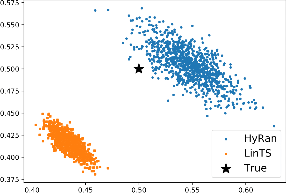
Figure 1: An illustration of the 1000 generated estimators of $\beta^{*}$ used in HyRan Bandit and LinTS at round $t=1000$, when $d=2$ and $N=5$. The points in blue and orange represent the generated HyRan and LinTS estimators, respectively. The black star in the plot represents the true parameter $\beta^{*}$.

Our proposed algorithm, HyRan Bandit, is presented in Algorithm 1. At each round $t$, the algorithm computes $X_{i,t}^{T}\widehat{\beta}_{t-1}$ for each arm $i\in[N]$ based on our estimator (6) and finds the arm $a_{t}$ with the maximum estimated reward. After pulling $a_{t}$ and observing the reward for the selected arm, the next step is to determine whether the contribution to the estimator is the ridge score (1) or the DR score (2). HyRan Bandit then samples the hybridization variable $h_{t}\in[N]$ from the multinomial distribution with probability ($\pi_{1,t},...,\pi_{N,t}$). This procedure determines whether the contexts and reward at round $t$ is added by  (1) or  (2). When $h_{t}$ is equal to $a_{t}$, we can observe the reward $\tilde{Y}_{h_{t},t}$ and compute the pseudo reward in (3). Therefore we include the round $t$ in $\Psi_{t}$, and use (2), otherwise we use  (1). When the contribution to the score function is determined, HyRan Bandit updates $\widehat{\beta}_{t}$ as in (6).

In order to compute $\widehat{\beta}_{t}$, the algorithm requires another imputation estimator $\check{\beta}_{t}$ to determine the pseudo reward in (3). In order to obtain the near-optimal regret bound, one must use an imputation estimator such that $\left\|\check{\beta}_{t}-\beta^{*}\right\|_{2}\leq N^{-1}$ holds after some explorations. For the definition of the imputation estimator $\check{\beta}_{t}$ used in our analysis, see Section A.5.1. Since $\check{\beta}_{t}$ is multiplied with mean zero random variable in (3) the unbiasedness of the estimator does not depend on the choice of $\check{\beta}_{t}$.

Discussion of the algorithm. The action selection in HyRan Bandit is greedy given the HyRan estimator. However the algorithm is not exploration-free since the HyRan estimator is generated randomly. Note that action selection in LinTS is also greedy given the sampled estimator. The estimator from LinTS represents a realization from a posterior distribution. Hence, exploration is embedded in the estimator through variability in the distribution. Similarly, in our method, exploration is embedded in the HyRan estimator. Our estimator represents a realization of random variables corresponding to a particular subset $\Psi_{t}$ out of all possible subsets. Therefore, exploration is inherent from the variability of randomization scheme. For the sake of illustrating inherent exploration, we purposely generate multiple estimators both for HyRan and LinTS in a given round. Note that both algorithms compute only a single estimator per round. In Figure 1, the points in blue represent the HyRan estimators of $\beta^{*}$ from many possible realizations of $\Psi_{t}$ due to the randomness of $h_{t}$. For LinTS, the points in orange represent the sampled estimators of $\beta^{*}$ from its posterior distribution. We observe that there is enough variability for our estimator as in LinTS.

5 MAIN RESULTS

In this section, we present our main theoretical results: the regret bound for HyRan Bandit (Theorem 5.1) and the estimation error bound of the proposed HyRan estimator (Theorem 5.4). We first provide the assumptions used throughout the analysis.

Assumption 1 (Boundedness).

For all $i\in[N]$ and $t\in[T]$, $\left\|X_{i,t}\right\|_{2}\leq 1$ and $\left\|\beta^{*}\right\|_{2}\leq 1$.

Assumption 2 (Sub-Gaussian noise).

For each $t$ and $i$, the noise $\eta_{i,t}$ is conditionally $\sigma$-sub-Gaussian for a fixed constant $\sigma\geq 0$, i.e, $\mathbb{E}\left[\left.\exp\left(\lambda\eta_{i,t}\right)\right|\mathcal{H}_{t}\right]\leq\exp(\lambda^{2}\sigma^{2}/2)$, for all $\lambda\in\mathbb{R}$.

Assumption 3 (Context stochasticity).

The set of context vectors $\mathcal{X}_{t}:=\{X_{i,t}\in\mathbb{R}^{d}:i\in[N]\}$ is independently drawn from unknown distribution $P_{\mathcal{X}}$ with $\lambda_{\min}(\mathbb{E}[\frac{1}{N}\sum_{i=1}^{N}X_{i,t}X_{i,t}^{T}])\geq\phi^{2}>0$, for all $t$.

Discussion of the assumptions. Assumptions 1 and 2 are standard in the stochastic contextual bandit literature (see e.g. Agrawal and Goyal (2013)). The same or similar assumption to Assumption 3 has been frequently used in the contextual bandit literature (Goldenshluger and Zeevi, 2013; Li et al., 2017; Bastani and Bayati, 2020; Oh et al., 2021; Kim et al., 2021). We emphasize that stochasticity is assumed for the entire context set and that we allow context vectors to be correlated in each round. We also emphasize that even under the stochasticity of contexts, achieving a regret bound sublinear in $d$ was only possible by resorting to the technique as used in SupLinUCB (Auer, 2002a) and its follow-up works.

The positive-definiteness on the average of the covariance matrix in Assumption 3 can be satisfied regardless of the number of arms - even when N = 1, e.g., when the context vector (s) is (are) drawn from the Uniform distribution or the truncated Gaussian distribution. Recently, Bastani et al. (2021); Kim et al. (2022) identified the practical cases where Assumption 3 holds. Technically, Assumption 3 is required to obtain the fast convergence rate in estimating linearly parametrized responses in Statistics (see e.g., Bühlmann and Van De Geer (2011)). In our work the assumption is used to obtain the fast convergence rate for the imputation estimator (Lemma B.3).

5.1 Regret Bound of HyRan Bandit

Under the assumptions above, we present the following regret bound for the HyRan Bandit algorithm.

Theorem 5.1.

Suppose Assumptions 1-3 hold and the total number of rounds $T$ satisfies

$$T\geq\mathcal{E}=\max\left\{\frac{8}{p}\log\frac{T}{\delta},C_{p,\sigma}N^{2}\phi^{-4}\log\frac{2T}{\delta}\right\},$$ (7)

where $C_{p,\sigma}:=\frac{8(2-p)}{(1-p)\sqrt{p}}+\frac{\sqrt{2}C\sigma}{p^{2}}+\frac{8}{\sqrt{p}}$ is a constant depending only on $p$ and $\sigma$. Set $\lambda_{t}:=d\log\frac{4t^{2}}{\delta}$. Then the total regret by time $T$ for HyRan Bandit is bounded by

$$\begin{split}R(T)\leq&2\mathcal{E}+4D_{p,\sigma}\sqrt{2T\log\frac{1}{\delta}}+3\delta D_{p,\sigma}\\ &+\frac{\left(16\sqrt{2}+8\right)D_{p,\sigma}}{\sqrt{p}}\sqrt{dT\log\frac{2T}{\delta}},\end{split}$$ (8)

with probability at least $1-8\delta$, where $D_{p,\sigma}:=1+\frac{4\sqrt{2}}{1-p}+\frac{\sigma}{p}$ is a constant depending only on $p$ and $\sigma$.

Discussion on the regret bound. The subsampling parameter $p\in(0,1)$ in HyRan Bandit is chosen independently with respect to $N$, $d$ or $T$ and does not affect the rate of our regret bound. The number of rounds $\mathcal{E}$ defined in (7) is required for the imputation estimator $\check{\beta}_{t}$ to obtain a suitable estimation error bound which is crucial to derive our self-normalized bound for HyRan estimator. The number of exploration rounds is $O(N^{2}\phi^{-4}\log T)$ which is only logarithmic in $T$ and is bounded by $O(\sqrt{dT\log T})$ when $\frac{T}{\log T}\geq N^{4}d^{-1}\phi^{-8}$. The value of $\phi^{-2}$ is $O(d)$ for many standard context distributions (see e.g., Lemma 5.2 in Kim et al. (2022)). As a result, the regret bound of HyRan Bandit is $O(\sqrt{dT\log T})$. Our bound is sharper than the existing regret bounds of $O(\sqrt{dT\log T\log N})\cdot\text{poly}(\log\log(NT))$ for VCL-SupLinUCB (Li et al., 2019) and $O(\sqrt{dT}\log^{3/2}(NT))$ for SupLinUCB (Chu et al., 2011), although direct comparison is not immediate due to difference in the assumptions used. It is important to note that the leading term in our regret bound does not depend on $N$ while the existing $\tilde{O}(\sqrt{dT})$ regret bounds all contain $N$ dependence in their leading terms. To our knowledge, the regret bound in Theorem 5.1 is the fastest rate among linear contextual bandit algorithms. Furthermore, we believe that HyRan Bandit is the first method achieving a regret that is sublinear in context dimension without using the widely used technique by Auer (2002a) and its variants (e.g., SupLinUCB).

Our regret bound in Theorem 5.1 is smaller than the existing lower bounds for the linear contextual bandits in Rusmevichientong and Tsitsiklis (2010); Lattimore and Szepesvári (2020) and Li et al. (2019). This is not a contradiction since the slightly different set of assumptions are used. i.e., Assumptions 3. We discuss this issue in Section 5.3 by proving a lower bound under Assumption 3, which matches with (8) up to a logarithmic factor.

5.2 Regret Decomposition

In the analysis of LinUCB and OFUL, an instantaneous regret is controlled by using the joint maximizer of the reward

$$(a_{t},\widehat{\beta}_{\textrm{ucb}})=\arg\max_{i\in[N],\beta\in\mathcal{C}_{t}}X_{i,t}^{T}\beta$$

where $\mathcal{C}_{t}$ is a high-probability confidence ellipsoid. Then, $\texttt{regret}(t)$ is typically decomposed as

$$\texttt{regret}(t)\leq\left\|\widehat{\beta}_{ucb}-\beta^{*}\right\|_{A_{t}}\left\|X_{a_{t},t}\right\|_{A_{t}^{-1}},$$ (9)

where $A_{t}:=\sum_{\tau=1}^{t}X_{a_{\tau},\tau}X_{a_{\tau},\tau}^{T}+\lambda I$. Each of the two terms on the right hand side in (9) has a $\sqrt{d}$ factor. In particular, $\sqrt{d}$ factor in the first term comes from the radius of $\mathcal{C}_{t}$. Hence, this results in $O(d)$ regret when combined.

In our work, we introduce new decomposition of regret that allows to avoid multiplicative terms. This decomposition allows for non-OFU based analysis for sharper dependence on dimensionality.

Lemma 5.2 (Regret decomposition).

Define the max-residual function for $x=(x_{1},\ldots,x_{N})\in\mathbb{R}^{d\times N}$ as $\Delta_{\widehat{\beta}}\left(x\right):=\max_{i\in[N]}|x_{i}^{T}(\widehat{\beta}-\beta^{*})|\,.$ For each $t\in[T]$, let $\mathcal{X}_{t}:=(X_{1,t},\ldots,X_{N,t})$ and denote $\mathcal{G}_{t}:=\cup_{\tau=1}^{t}\{\mathcal{X}_{\tau},\widehat{\beta}_{\tau}\}$. Then for $t\geq 1$,

$$\begin{split}&\texttt{regret}(t+1)\\ &\leq 2\left\{\Delta_{\widehat{\beta}_{t}}\left(\mathcal{X}_{t+1}\right)-\mathbb{E}\left[\left.\Delta_{\widehat{\beta}_{t}}\left(\mathcal{X}_{t+1}\right)\right|\mathcal{G}_{t}\right]\right\}\\ &+2\left\{\mathbb{E}\left[\left.\Delta_{\widehat{\beta}_{t}}\left(\mathcal{X}_{t+1}\right)\right|\mathcal{G}_{t}\right]-\frac{1}{\left|\Psi_{t}\right|}\sum_{\tau\in\Psi_{t}}\Delta_{\widehat{\beta}_{t}}\left(\mathcal{X}_{\tau}\right)\right\}\\ &+\frac{2}{\sqrt{\left|\Psi_{t}\right|}}\left\|\widehat{\beta}_{t}-\beta^{*}\right\|_{V_{t}},\end{split}$$ (10)

where

$$V_{t}:=\sum_{\tau\in\Psi_{t}}\sum_{i=1}^{N}X_{i,\tau}X_{i,\tau}^{T}+\sum_{\tau\notin\Psi_{t}}X_{a_{\tau},\tau}X_{a_{\tau},\tau}^{T}+\lambda_{t}I.$$

The decomposition of the expected regret given in (10) directly bounds the regret by approximating the max-residual with $t+1$-th contexts $\mathcal{X}_{t+1}$ to that with the average over the contexts in round $\tau\in\Psi_{t}$, which is bounded by the self-normalized bound for HyRan estimator. This approximation yields two additive terms: the difference between the max-residual function and its expectation $(\Delta_{\widehat{\beta}_{t}}\left(\mathcal{X}_{t+1}\right)-\mathbb{E}\left[\left.\Delta_{\widehat{\beta}_{t}}\left(\mathcal{X}_{t+1}\right)\right|\mathcal{G}_{t}\right])$, and the difference between the expectation over the context distribution and its empirical distribution ($\mathbb{E}\left[\left.\Delta_{\widehat{\beta}_{t}}\left(\mathcal{X}_{t+1}\right)\right|\mathcal{G}_{t}\right]-\frac{1}{\left|\Psi_{t}\right|}\sum_{\tau\in\Psi_{t}}\Delta_{\widehat{\beta}_{t}}\left(\mathcal{X}_{\tau}\right)$). The bound becomes tighter as the size of $\Psi_{t}$ increases, because we can use more contexts for the approximation.

The decomposition is insightful in that the regret from suboptimal arm selections is incurred due to poor estimate, thus can be bounded by the quantities involving the maximum residual. To bound the maximum residual, SupLinUCB and their variants that achieve $\tilde{O}(\sqrt{dT})$ regret bound handle the maximum residual with the union of $N\times T$ probability inequalities, and this gives $\log N$ term in the regret bound. But in Lemma 5.2, we use the fact that the maximum residual is bounded by a sum of residuals. The sum of residuals can be shown to be bounded by the self-normalized bound for our estimator in (6). This replacement is possible since our novel estimator uses all contexts for some subsampled rounds. In this way, we can use only $T$ probability inequalities and eliminate the $N$ independence on the leading term of the regret bound. We emphasize that the decomposition yields the self-normalized bound of our new estimator, not any estimator using the contexts of selected arms only (e.g. ridge estimator for OFUL). Our bound is normalized with the hybrid Gram matrix $V_{t}$, not that of selected contexts.

To bound the terms in the decomposed instantaneous regret (10), we see that the first term is bounded by using Azuma’s inequality. We bound the second and third term using Lemma 5.3 and Theorem 5.4, respectively. Lemma 5.3 adopts the empirical theories on the distribution of the contexts.

Lemma 5.3.

Suppose Assumptions 1-3 hold. For each $t\in[T]$, and $L>0$, conditioned on $\Psi_{t}$, with probability at least $1-\delta/T$,

$$\sup_{\left\|\beta_{1}-\beta^{*}\right\|_{2}\leq L}\left|\mathbb{E}\left[\left.\Delta_{\beta_{1}}\left(\mathcal{X}_{t+1}\right)\right|\mathcal{G}_{t}\right]-\frac{1}{\left|\Psi_{t}\right|}\sum_{\tau\in\Psi_{t}}\Delta_{\beta_{1}}\left(\mathcal{X}_{\tau}\right)\right|$$

$$\leq\frac{3L\delta}{2T}+4L\sqrt{\frac{1}{\left|\Psi_{t}\right|}}\sqrt{d\log\frac{2T}{\delta}}.$$

In the following theorem, we present the self-normalized bound for the compound estimator which allows us to bound the last term in (10).

Theorem 5.4 (A self-normalized bound for HyRan estimator).

Suppose Assumptions 1-3 hold. Let $\widehat{\beta}_{t}$ be the estimator defined in (6) and $p\in(0,1)$ be a constant used in (5). Then with probability at least $1-6\delta$,

$$\left\|\widehat{\beta}_{t}-\beta^{*}\right\|_{V_{t}}\leq\sqrt{\lambda_{t}}+\left(\frac{4\sqrt{2}}{1-p}+\frac{\sigma}{p}\right)\sqrt{d\log\frac{4t^{2}}{\delta}},$$ (11)

for all $t\geq\max\left\{\frac{8}{p}\log\frac{T}{\delta},C_{p,\sigma}N^{2}\phi^{-4}\log\frac{2T}{\delta}\right\}$, where $C_{p,\sigma}>0$ is a constant depending only on $p$ and $\sigma$.

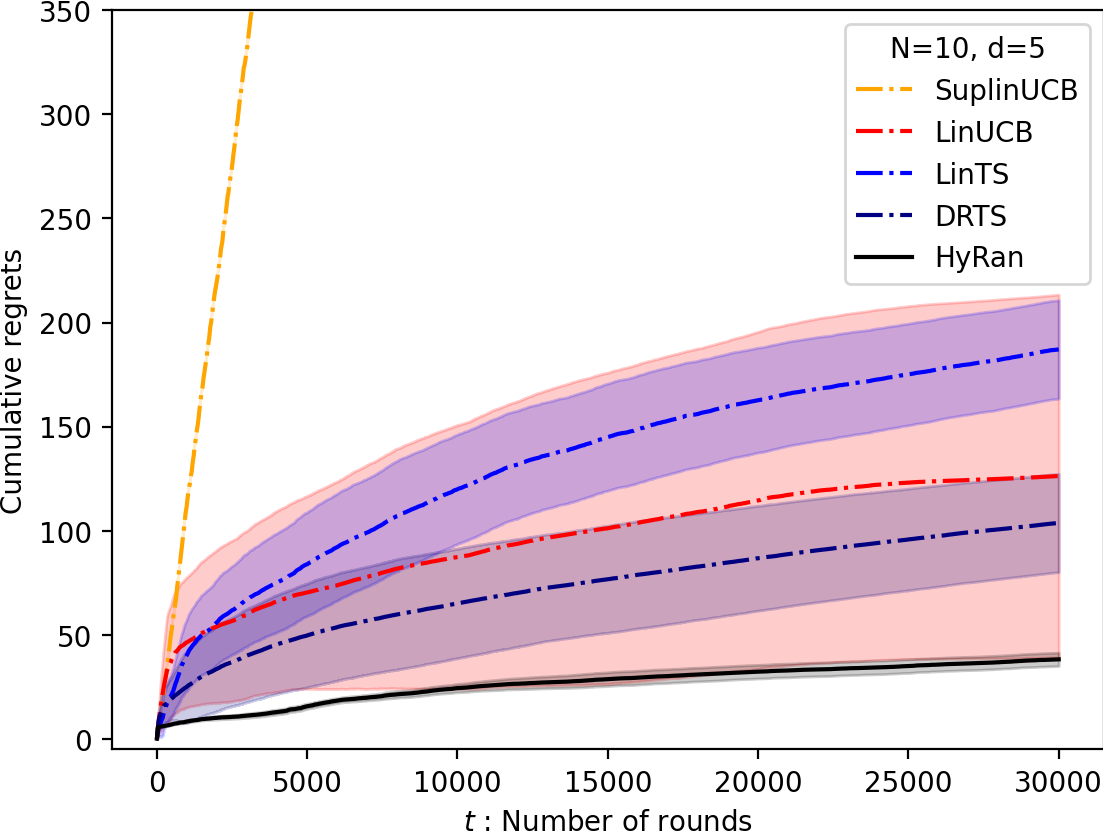
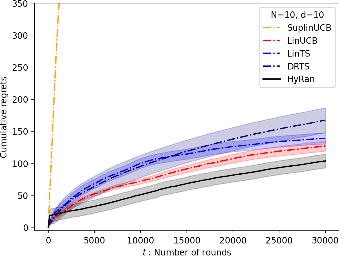
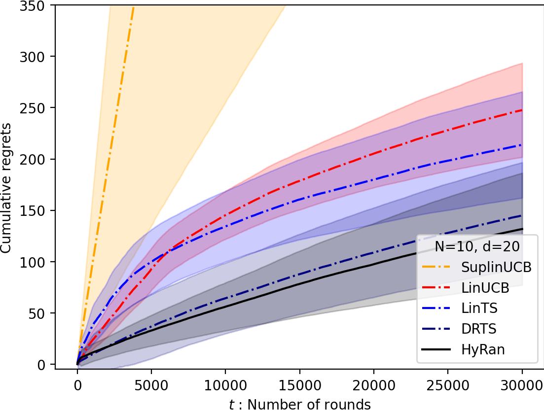
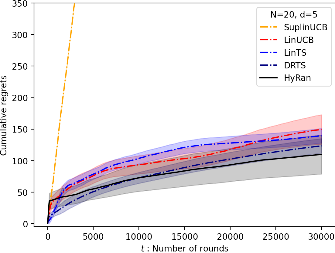
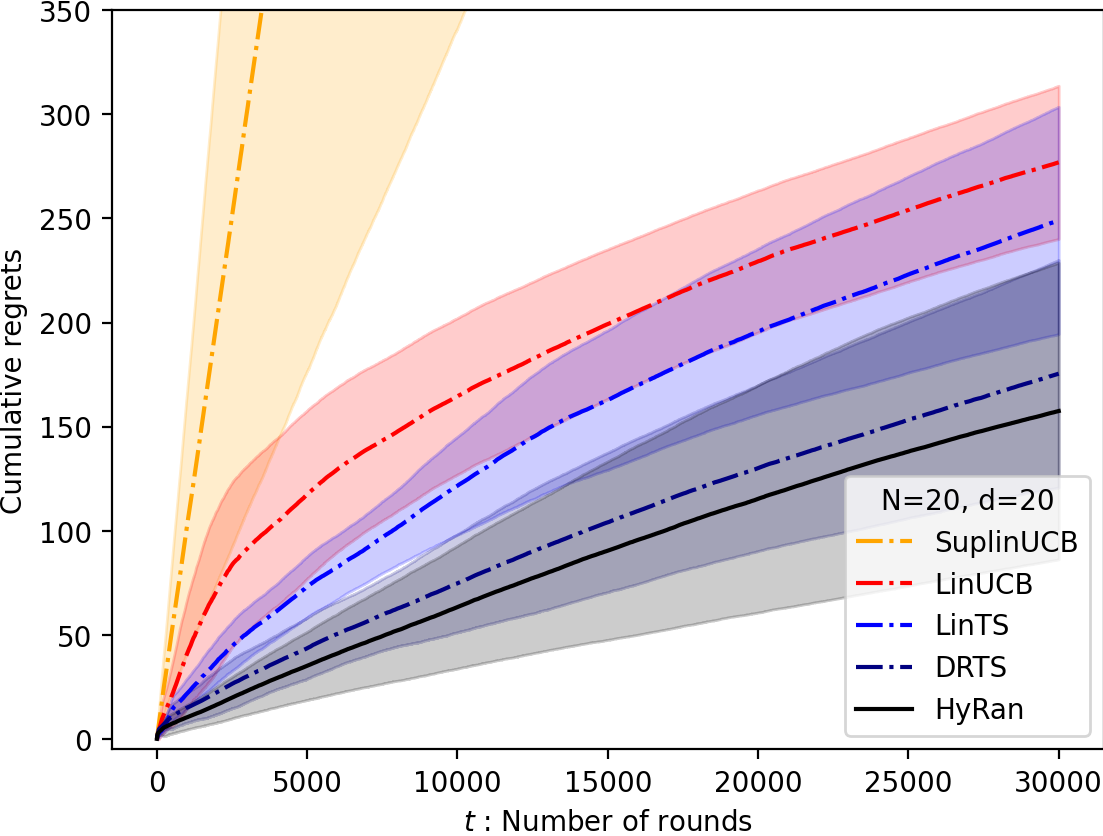
Figure 2: A comparison of cumulative regrets of SupLinUCB, LinTS, LinUCB, DRTS and HyRan Bandit. Each curve shows the cumulative regret as a function of rounds, averaged over 20 repeated experiments. The scale of $y$-axis is set to be equivalent in each row for the comparison of the regret as $d$ increases. The standard deviations of SupLinUCB in $d=5$ and $d=10$ are too large to present and omitted.

Theorem 5.4 is a self-normalized bound for the HyRan estimator, which is a crucial element in our regret analysis. Compared to the widely-used self-normalization bound (Theorem 2 in Abbasi-Yadkori et al. (2011)) in the contextual bandit literature, the estimation error bound (11) is self-normalized by the covariance matrix constructed by the contexts of all arms, not just selected contexts. The self-normalized bound is derived by using the pairs of pseudo reward $\tilde{Y}_{i,\tau}$ defined in (3) and contexts $X_{i,\tau}$ for all arms $i\in[N]$ and $\tau\in\Psi_{t}$, instead of using just the pairs of selected arms. The full usage of pseudo rewards and contexts enables us to take advantage of the new decomposition of the regret in (10), which derives a $O(\sqrt{dT\log T})$ regret bound.

The last concern regarding our regret bound is the size of $\Psi_{t}$. To obtain a regret bound sublinear to $T$, we need to make sure that the sum of the subsampled rounds satisfies $\sum_{t=1}^{T}\left|\Psi_{t}\right|^{-1/2}=O(\sqrt{T})$. In the following Lemma, we show this by proving that the size of the selected subset $\Psi_{t}$ is $\Omega(t)$ with high probability.

Lemma 5.5.

Let $\Psi_{t}$ be a subset of $[t]$ determined by the Algorithm 1 at round $t$. For any $\epsilon\in(0,1)$, with probability at least $1-\delta$,

$$\left|\Psi_{t}\right|\geq\epsilon pt,$$ (12)

for all $t\geq\frac{2}{p\left(1-\epsilon\right)^{2}}\log\frac{T}{\delta}$.

With (12), we guarantee the rate of the regret bound is sub-linear with respect to the total round $T$.

5.3 Matching Lower Bound

Regarding the lower bounds of the linear contextual bandit, a $\Omega(d\sqrt{T})$ bound has been proven for linear bandits with infinitely many arms (Dani et al., 2008; Rusmevichientong and Tsitsiklis, 2010; Lattimore and Szepesvári, 2020). When the number of arms is finite, the derived lower bound of the cumulative regret is $\Omega(\sqrt{dT})$ (Chu et al., 2011). Recently in Li et al. (2019), a lower bound $\Omega(\sqrt{dT\log T\log N})$ was shown when $N\leq 2^{d/2}$. These lower bounds are derived by finding the settings of contexts and parameters that make the algorithm difficult to reduce the regret. However, the problem settings of the existing lower bounds do not satisfy Assumptions 3 in our problem setting. In the following theorem, we prove a lower bound which is valid under Assumptions 1-3.

Theorem 5.6.

Assume $2\leq d\leq N<\infty$ and $T\geq d/4$. Then there exists a distribution of contexts, $\mathcal{P}_{\mathcal{X}}$, a distribution of noise, $\eta_{i,t}$ and $\beta^{*}$, which satisfies Assumptions 1-3 and for any bandit algorithms that selects $a_{t}$,

$$\mathbb{E}_{\beta^{*}}R(T)\geq\frac{1}{8}\sqrt{dT}.$$ (13)

We prove that the rate of $\Omega(\sqrt{dT})$ cannot be improved even under the stochastic assumptions on contexts (e.g., Assumption 3). The lower bound in Theorem 5.6 matches with our regret upper bound for HyRan Bandit established in Theorem 5.1 up to the logarithmic factor. Therefore, our proposed algorithm HyRan Bandit is provably near-optimal, i.e., optimal up to the logarithmic factor. To our knowledge, all of the existing near-optimal linear contextual bandit algorithms are based on the framework of Auer (2002a) (e.g., SupLinUCB and VCL-SupLinUCB). Our proposed algorithm is the first algorithm that achieves near-optimality without relying on this existing framework.

Despite the lower bound is derived under Assumption 3 related to the factor $\phi>0$ , our lower bound (13) does not have $\phi$. This is because the lower bound depends only on the number of orthogonal vectors in the contexts space $\mathbb{R}^{d}$, not the value of $\phi>0$.

6 NUMERICAL EXPERIMENTS

In this section, we compare the performances of the five linear contextual bandit algorithms: SupLinUCB (Chu et al., 2011), LinUCB (Li et al., 2010), LinTS (Agrawal and Goyal, 2013), DRTS (Kim et al., 2021) and our proposed method, HyRan Bandit. For simulation, the number of arms $N$ is set to $10$ or $20$, and the dimension of contexts $d$ is set to $5$, $10$ and $20$. Let $X_{i,t}^{(1)},\ldots,X_{i,t}^{(d)}$ be the $d$ elements of a context $X_{i,t}$. For $j=1,\ldots,d-1$, we independently generate $(X_{1,t}^{(j)},\cdots,X_{N,t}^{(j)})$ from a normal distribution $\mathcal{N}(\mu_{N},V_{N})$ with mean $\mu_{10}\!=\!(-10,-8,\cdots,-2,2,\cdots 8,-10)^{T}$, or $\mu_{20}=(-20,-18,\cdots,-2,2,\cdots,18,20)^{T}$. To impose correlation among each arms the covariance matrix $V_{N}\in\mathbb{R}^{N\times N}$ is set as $V(i,i)=1$ for every $i$ and $V(i,k)=0.5$ for every $i\neq k$. Then, for each arm $i\in[N]$, we randomly select a generated element $X_{i,t}^{(j)}$ and append it to the last element, i.e. $X_{i,t}^{(d)}$ is the same as one of $X_{i,t}^{(1)},\ldots,X_{i,t}^{(d-1)}$. This setting is to impose a severe multicollinearity on each contexts. Finally, we truncated the sampled contexts to satisfy $\|X_{i,t}\|_{2}\leq 1$. To generate the stochastic rewards, we sample $\eta_{i,t}$ independently from $\mathcal{N}(0,1)$. Each element of $\beta^{*}$ is sampled from a uniform distribution, $\mathcal{U}(-{1}/{\sqrt{d}},{1}/{\sqrt{d}})$ at the beginning of each instance and stays fixed during experiments. About the set of hyperparameters, LinTS, LinUCB, SupLinUCB and DRTS searches $\alpha$ (or $v$) in $\{0.001,0.01,0.1,1\}$. In HyRan Bandit we set $\lambda_{t}:=d\log(t+1)^{2}$ to be consistent with the theoretical results and $p$ to be in {0.5,0.65,0.8,0.95}. We optimize the hyperparameters over the grid set and report the best performance for each algorithm. Figure 2 shows the average of the cumulative regrets over the horizon length $T=30000$ with 20 repeated experiments. The experimental results demonstrate that HyRan Bandit performs better than the benchmarks in all of the cases and shows superior performances as the context dimension increases. The worst performance of SupLinUCB is mainly because its estimator does not include rewards in exploitation rounds.

7 CONCLUSION

We address a long-standing research question of whether a practical algorithm can achieve near-optimality for linear contextual bandits. We show that our proposed algorithm achieves $\tilde{O}(\sqrt{dT})$ regret upper bound which matches the lower bound under our problem setting. We empirically evaluate our algorithm to support our theoretical claims and show that the practical performance of our algorithm outperforms the existing methods, hence achieving both provable near-optimality and practicality.

Acknowledgements

This work is supported by the National Research Foundation of Korea (NRF) grant funded by the Korea government (MSIT, No.2020R1A2C1A01011950) (WK and MCP) and (MSIT, No. 2022R1C1C1006859) (MO), and also supported by Naver (MO) and Hyundai Chung Mong-koo scholarship foundation (WK).

Appendix A MISSING PROOFS

A.1 Technical lemmas

Lemma A.1.

Lee et al. (2016, Lemma 2.3) Let $\left\{N_{t}\right\}$ be a martingale on a Hilbert space $(\mathcal{H},\left\|\cdot\right\|_{\mathcal{H}})$. Then there exists a $\mathbb{R}^{2}$-valued martingale $\left\{M_{t}\right\}$ such that for any time $t\geq 0$, $\left\|M_{t}\right\|_{2}=\left\|N_{t}\right\|_{\mathcal{H}}$ and $\left\|M_{t+1}-M_{t}\right\|_{2}=\left\|N_{t+1}-N_{t}\right\|_{\mathcal{H}}$.

Lemma A.2.

(Azuma-Hoeffding) If a super-martingale $(Y_{t};t\geq 0)$ corresponding to filtration $\mathcal{F}_{t}$, satisfies $\left|Y_{t}-Y_{t-1}\right|\leq c_{t}$ for some constant $c_{t}$, for all $t=1,\ldots,T$, then for any $a\geq 0$,

$$\mathbb{P}\left(Y_{T}-Y_{0}\geq a\right)\leq e^{-\frac{a^{2}}{2\sum_{t=1}^{T}c_{t}^{2}}}.$$

A.2 Proof of Theorem 5.1

Proof.

[Step 1. Regret decomposition] For each $t\in[T]$, define the event

$$\begin{split}A_{t}&:=\left\{\left|\Psi_{t}\right|>\frac{1}{2}pt\right\},\\ B_{t}&:=\left\{\left\|\widehat{\beta}_{t}-\beta^{*}\right\|_{V_{t}}\leq\sqrt{\lambda_{t}}+\left(\frac{4\sqrt{2}}{1-p}+\frac{\sigma}{p}\right)\sqrt{d\log\frac{4t^{2}}{\delta}}\right\},\\ C_{t}&:=\left\{\left\|\widehat{\beta}_{t}-\beta^{*}\right\|_{2}\leq 1+\frac{4\sqrt{2}}{1-p}+\frac{\sigma}{p}:=D_{p,\sigma}\right\}.\end{split}$$

The three events have an explicit relationship as follows: In the proof of Theorem 5.4, Lemma 5.5 and Lemma A.3, the event $B_{t}$ requires $A_{t}$, i.e. $A_{t}\subseteq B_{t}$. Under the event $B_{t}$, setting $\lambda_{t}=d\log\frac{4t^{2}}{\delta}$ gives

$$\left\|\widehat{\beta}_{t}-\beta^{*}\right\|_{2}\leq \sqrt{\left(\widehat{\beta}_{t}-\beta^{*}\right)^{T}V_{t}^{\frac{1}{2}}V_{t}^{-1}V_{t}^{\frac{1}{2}}\left(\widehat{\beta}_{t}-\beta^{*}\right)}$$

$$\leq \sqrt{\lambda_{\max}\left(V_{t}^{-1}\right)}\left\|\widehat{\beta}_{t}-\beta^{*}\right\|_{V_{t}}$$

$$\leq \lambda_{t}^{-\frac{1}{2}}\left(\sqrt{\lambda_{t}}+\left(\frac{4\sqrt{2}}{1-p}+\frac{\sigma}{p}\right)\sqrt{d\log\frac{4t^{2}}{\delta}}\right)$$

$$\leq D_{p,\sigma},$$

which implies $C_{t}$. Set $\mathcal{E}:=\max\left\{\frac{8}{p}\log\frac{T}{\delta},C_{p,\sigma}N^{2}\phi^{-4}\log\frac{2T}{\delta}\right\}$, where $C_{p,\sigma}$ is defined in (25). By Theorem 5.4 we have

$$\mathbb{P}\left(\bigcap_{t\geq\mathcal{E}}\left\{A_{t}\cap B_{t}\cap C_{t}\right\}\right)\geq 1-6\delta.$$ (14)

By Lemma 5.2, for each $t\geq\mathcal{E}$,

$$\texttt{regret}(t) \leq 2\left\{\Delta_{\widehat{\beta}_{t-1}}\left(\mathcal{X}_{t}\right)-\mathbb{E}\left[\left.\Delta_{\widehat{\beta}_{t-1}}\left(\mathcal{X}_{t}\right)\right|\mathcal{G}_{t-1}\right]\right\}$$

$$+2\left\{\mathbb{E}\left[\left.\Delta_{\widehat{\beta}_{t-1}}\left(\mathcal{X}_{t}\right)\right|\mathcal{G}_{t-1}\right]-\frac{1}{\left|\Psi_{t-1}\right|}\sum_{\tau\in\Psi_{t-1}}\Delta_{\widehat{\beta}_{t-1}}\left(\mathcal{X}_{\tau}\right)\right\}$$

$$+\frac{2}{\sqrt{\left|\Psi_{t-1}\right|}}\left\|\beta^{*}-\widehat{\beta}_{t-1}\right\|_{V_{t-1}}.$$

Let

$$\begin{split}R_{1}(t):=&2\left\{\Delta_{\widehat{\beta}_{t-1}}\left(\mathcal{X}_{t}\right)-\mathbb{E}\left[\left.\Delta_{\widehat{\beta}_{t-1}}\left(\mathcal{X}_{t}\right)\right|\mathcal{G}_{t-1}\right]\right\},\\ R_{2}(t):=&2\left\{\mathbb{E}\left[\left.\Delta_{\widehat{\beta}_{t-1}}\left(\mathcal{X}_{t}\right)\right|\mathcal{G}_{t-1}\right]-\frac{1}{\left|\Psi_{t-1}\right|}\sum_{\tau\in\Psi_{t-1}}\Delta_{\widehat{\beta}_{t-1}}\left(\mathcal{X}_{\tau}\right)\right\},\\ R_{3}(t):=&\frac{2}{\sqrt{\left|\Psi_{t-1}\right|}}\left\|\beta^{*}-\widehat{\beta}_{t-1}\right\|_{V_{t-1}}.\end{split}$$ (15)

[Step 2. Bounding $R_{1}(t)$] Let us bound $R_{1}(t)$. Since the event $C_{t}$ is $\mathcal{G}_{t}$-measurable for each $t\in[T]$, we have

$$R_{1}(t)\mathbb{I}\left(C_{t-1}\right)=2\left\{\Delta_{\widehat{\beta}_{t-1}}\left(\mathcal{X}_{t}\right)\mathbb{I}\left(C_{t-1}\right)-\mathbb{E}\left[\left.\Delta_{\widehat{\beta}_{t-1}}\left(\mathcal{X}_{t}\right)\mathbb{I}\left(C_{t-1}\right)\right|\mathcal{G}_{t-1}\right]\right\}.$$

By Assumption 1,

$$\Delta_{\widehat{\beta}_{t-1}}\left(\mathcal{X}_{t}\right)\mathbb{I}\left(C_{t-1}\right):= \max_{i\in[N]}\left|X_{i,t}^{T}\left(\widehat{\beta}_{t-1}-\beta^{*}\right)\right|\mathbb{I}\left(C_{t-1}\right)$$

$$\leq \max_{i\in[N]}\left\|X_{i,t}\right\|_{2}\left\|\widehat{\beta}_{t-1}-\beta^{*}\right\|_{2}\mathbb{I}\left(C_{t-1}\right)$$

$$\leq \left\|\widehat{\beta}_{t-1}-\beta^{*}\right\|_{2}\mathbb{I}\left(C_{t-1}\right)$$

$$\leq D_{p,\sigma}.$$

Thus, $\left|R_{1}(t)\mathbb{I}\left(C_{t-1}\right)\right|\leq 4D_{p,\sigma}$. Since $R_{1}(t)\mathbb{I}\left(C_{t-1}\right)$ is $\mathcal{G}_{t}$-measurable and

$$\mathbb{E}\left[\left.R_{1}(t)\mathbb{I}\left(C_{t-1}\right)\right|\mathcal{G}_{t-1}\right]=0,$$

we can use Lemma A.2 to have

$$\sum_{t>\mathcal{E}}R_{1}(t)\mathbb{I}\left(C_{t-1}\right)\leq 4D_{p,\sigma}\sqrt{2T\log\frac{1}{\delta}},$$ (16)

with probability at least $1-\delta$.

[Step 3. Bounding $R_{2}(t)$] Now we bound $R_{2}(t)$. By Lemma 5.3 with probability at least $1-\delta/T$,

$$R_{2}(t)\mathbb{I}\left(A_{t-1}\cap C_{t-1}\right) \leq 2\mathbb{I}\left(A_{t-1}\right)\!\sup_{\left\|\beta_{1}-\beta^{*}\right\|_{2}\leq D_{p,\sigma}}\!\left|\mathbb{E}\left[\left.\Delta_{\beta_{1}}\left(\mathcal{X}_{t}\right)\right|\mathcal{G}_{t-1}\right]-\frac{1}{\left|\Psi_{t-1}\right|}\sum_{\tau\in\Psi_{t-1}}\Delta_{\beta_{1}}\left(\mathcal{X}_{\tau}\right)\right|$$

$$\leq\left(\frac{3\delta D_{p,\sigma}}{T}+8D_{p,\sigma}\sqrt{\frac{1}{\left|\Psi_{t-1}\right|}}\sqrt{d\log\frac{2T}{\delta}}\right)\mathbb{I}\left(A_{t-1}\right)$$

$$\leq\frac{3\delta D_{p,\sigma}}{T}+8D_{p,\sigma}\sqrt{\frac{2}{pt}}\sqrt{d\log\frac{2T}{\delta}}.$$

Thus, with probability at least $1-\delta$,

$$\sum_{t>\mathcal{E}}R_{2}(t)\mathbb{I}\left(A_{t-1}\cap C_{t-1}\right)\leq 3\delta D_{p,\sigma}+\frac{16\sqrt{2}D_{p,\sigma}}{\sqrt{p}}\sqrt{dT\log\frac{2T}{\delta}}.$$ (17)

[Step 4. Bounding $R_{3}(t)$] To bound $R_{3}(t)$,

$$R_{3}(t)\mathbb{I}\left(A_{t-1}\cap B_{t-1}\right)\leq \frac{2\sqrt{2}}{\sqrt{pt}}\left(1+\frac{4C}{1-p}+\frac{\sigma}{p}\right)\sqrt{d\log\frac{4t^{2}}{\delta}}$$

$$= \frac{2\sqrt{2}}{\sqrt{pt}}D_{p,\sigma}\sqrt{d\log\frac{4t^{2}}{\delta}}.$$

and

$$\sum_{t>\mathcal{E}}R_{3}(t)\mathbb{I}\left(A_{t-1}\cap B_{t-1}\right)\leq\frac{8D_{p,\sigma}}{\sqrt{p}}\sqrt{dT\log\frac{2T}{\delta}},$$ (18)

holds almost surely.

[Step 5. Collecting the bounds] For any $x>2\mathcal{E}$,

$$\mathbb{P}\left(R(T)>x\right) \leq\mathbb{P}\left(2\mathcal{E}+\sum_{t>\mathcal{E}}\texttt{regret}(t)>x\right)$$

$$=\mathbb{P}\left(2\mathcal{E}+\sum_{t>\mathcal{E}}R_{1}(t)+R_{2}(t)+R_{3}(t)>x\right)$$

$$\leq\mathbb{P}\!\left(2\mathcal{E}\!+\!\sum_{t>\mathcal{E}}R_{1}(t)\mathbb{I}\left(C_{t-1}\right)\!+\!R_{2}(t)\mathbb{I}\left(A_{t-1}\!\cap\!C_{t-1}\right)\!+\!R_{3}(t)\mathbb{I}\left(A_{t-1}\!\cap\!B_{t-1}\right)>x\right)$$

$$\quad+\mathbb{P}\left(\bigcup_{t\geq\mathcal{E}}\left\{A_{t}^{c}\cup B_{t}^{c}\cup C_{t}^{c}\right\}\right)$$

$$\leq\mathbb{P}\!\left(2\mathcal{E}\!+\!\sum_{t>\mathcal{E}}R_{1}(t)\mathbb{I}\left(C_{t-1}\right)\!+\!R_{2}(t)\mathbb{I}\left(A_{t-1}\!\cap\!C_{t-1}\right)\!+\!R_{3}(t)\mathbb{I}\left(A_{t-1}\!\cap\!B_{t-1}\right)>x\right)$$

$$\quad+6\delta,$$

where the last inequality holds due to (14). Setting

$$x=2\mathcal{E}+4D_{p,\sigma}\sqrt{2T\log\frac{1}{\delta}}+3\delta D_{p,\sigma}+\frac{16\sqrt{2}D_{p,\sigma}}{\sqrt{p}}\sqrt{dT\log\frac{2T}{\delta}}+\frac{8D_{p,\sigma}}{\sqrt{p}}\sqrt{dT\log\frac{2T}{\delta}},$$

gives

$$\mathbb{P}\left(R(T)>x\right)\leq 6\delta+\mathbb{P}\left(\sum_{t>\mathcal{E}}R_{1}(t)\mathbb{I}\left(C_{t-1}\right)>4D_{p,\sigma}\sqrt{2T\log\frac{1}{\delta}}\right)$$

$$+\mathbb{P}\left(\sum_{t>\mathcal{E}}R_{2}(t)\mathbb{I}\left(A_{t-1}\cap C_{t-1}\right)>3\delta D_{p,\sigma}+\frac{16\sqrt{2}D_{p,\sigma}}{\sqrt{p}}\sqrt{dT\log\frac{2T}{\delta}}\right)$$

$$+\mathbb{P}\left(\sum_{t>\mathcal{E}}R_{3}(t)\mathbb{I}\left(A_{t-1}\cap C_{t-1}\right)>\frac{8D_{p,\sigma}}{\sqrt{p}}\sqrt{dT\log\frac{2T}{\delta}}\right)$$

$$\leq 8\delta,$$

where the inequality holds due to (15)-(18). ∎

A.3 Proof of Lemma 5.2

Proof.

By the definition of $a_{t}$, we have

$$\begin{split}\texttt{regret}(t+1)=&\left(X_{a_{t+1}^{*},t+1}-X_{a_{t+1},t+1}\right)^{T}\left(\beta^{*}-\widehat{\beta}_{t}\right)+\left(X_{a_{t+1}^{*},t+1}-X_{a_{t+1},t+1}\right)^{T}\widehat{\beta}_{t}\\ \leq&\left(X_{a_{t+1}^{*},t+1}-X_{a_{t+1},t+1}\right)^{T}\left(\beta^{*}-\widehat{\beta}_{t}\right)\\ \leq&2\max_{i\in[N]}\left|X_{i,t+1}^{T}\left(\widehat{\beta}_{t}-\beta^{*}\right)\right|,\end{split}$$

which gives $\texttt{regret}(t+1)\leq 2\Delta_{\widehat{\beta}_{t}}\left(\mathcal{X}_{t+1}\right)$. Adding and subtracting $\mathbb{E}\left[\left.\Delta_{\widehat{\beta}_{t}}\left(\mathcal{X}_{t+1}\right)\right|\mathcal{G}_{t}\right]$ and $\frac{1}{\left|\Psi_{t}\right|}\sum_{\tau\in\Psi_{t}}\Delta_{\widehat{\beta}_{t}}\left(\mathcal{X}_{\tau}\right)$, we only need to show,

$$\frac{1}{\left|\Psi_{t}\right|}\sum_{\tau\in\Psi_{t}}\Delta_{\widehat{\beta}_{t}}\left(\mathcal{X}_{\tau}\right)\leq\frac{1}{\sqrt{\left|\Psi_{t}\right|}}\left\|\widehat{\beta}_{t}-\beta^{*}\right\|_{V_{t}},$$

for (10). By the Cauchy-Schwartz inequality,

$$\begin{split}\sum_{\tau\in\Psi_{t}}\Delta_{\widehat{\beta}_{t}}\left(\mathcal{X}_{\tau}\right)&\leq\sqrt{\left|\Psi_{t}\right|}\sqrt{\sum_{\tau\in\Psi_{t}}\left\{\Delta_{\widehat{\beta}_{t}}\left(\mathcal{X}_{\tau}\right)\right\}^{2}}\\ &=\sqrt{\left|\Psi_{t}\right|}\sqrt{\sum_{\tau\in\Psi_{t}}\max_{i\in[N]}\left\{X_{i,\tau}^{T}\left(\widehat{\beta}_{t}-\beta^{*}\right)\right\}^{2}}\\ &\leq\sqrt{\left|\Psi_{t}\right|}\sqrt{\sum_{\tau\in\Psi_{t}}\sum_{i=1}^{N}\left\{X_{i,\tau}^{T}\left(\widehat{\beta}_{t}-\beta^{*}\right)\right\}^{2}}\\ &\leq\sqrt{\left|\Psi_{t}\right|}\sqrt{\left(\widehat{\beta}_{t}\!-\!\beta^{*}\right)^{T}\!V_{t}\left(\widehat{\beta}_{t}\!-\!\beta^{*}\right)},\end{split}$$

where the last inequality holds with the fact that $V_{t}\succeq\sum_{\tau\in\Psi_{t}}\sum_{i=1}^{N}X_{i,\tau}X_{i,\tau}^{T}$. ∎

A.4 Proof of Lemma 5.3

Proof.

Let us fix $t\in[T]$ and $\Psi_{t}\subseteq[t]$. By Assumption 3, $\mathcal{X}_{t}$ is independent with $\mathcal{G}_{t-1}$. Thus,

$$\mathbb{E}\left[\left.\Delta_{\beta_{1}}\left(\mathcal{X}_{t}\right)\right|\mathcal{G}_{t-1}\right]=\mathbb{E}_{X}\left[\Delta_{\beta_{1}}\left(X\right)\right],$$

where $X\in\mathbb{R}^{d\times N}$ arises from $P_{X}$ defined in Assumption 3. For any $x>0$ and $\theta>0$,

$$\mathbb{P}\left(\left.\sup_{\left\|\beta_{1}-\beta^{*}\right\|_{2}\leq L}\left|\mathbb{E}\left[\left.\Delta_{\beta_{1}}\left(\mathcal{X}_{t}\right)\right|\mathcal{G}_{t-1}\right]-\frac{1}{\left|\Psi_{t}\right|}\sum_{\tau\in\Psi_{t}}\Delta_{\beta_{1}}\left(\mathcal{X}_{t}\right)\right|>x\right|\Psi_{t}\right)$$

$$\leq\exp\left(-\theta x\right)\mathbb{E}\left[\left.\exp\left(\theta\sup_{\left\|\beta_{1}-\beta^{*}\right\|_{2}\leq L}\left|\mathbb{E}_{X}\left[\Delta_{\beta_{1}}\left(\mathcal{X}_{t}\right)\right]-\frac{1}{\left|\Psi_{t}\right|}\sum_{\tau\in\Psi_{t}}\Delta_{\beta_{1}}\left(\mathcal{X}_{t}\right)\right|\right)\right|\Psi_{t}\right].$$

Let $\tau_{1}\leq\tau_{2},\ldots\leq\tau_{\left|\Psi_{t}\right|}$ be an ordered round in $\Psi_{t}$. Then by Assumption 3, $\mathcal{X}_{\tau_{1}},\ldots,\mathcal{X}_{\tau_{\left|\Psi_{t}\right|}}$ are IID random variables and we can use the symmetrization lemma (van der Vaart and Wellner, 1996, Lemma 2.3.1) to have

$$\begin{split}\mathbb{E}&\left[\exp\left(\theta\sup_{\left\|\beta_{1}-\beta^{*}\right\|_{2}\leq L}\left|\mathbb{E}_{X}\left[\Delta_{\beta_{1}}\left(\mathcal{X}_{t}\right)\right]-\frac{1}{\left|\Psi_{t}\right|}\sum_{\tau\in\Psi_{t}}\Delta_{\beta_{1}}\left(\mathcal{X}_{t}\right)\right|\right)\right]\\ &\leq\mathbb{E}\left[\exp\left(2\theta\sup_{\left\|\beta_{1}-\beta^{*}\right\|_{2}\leq L}\left|\frac{1}{\left|\Psi_{t}\right|}\sum_{n=1}^{\left|\Psi_{t}\right|}\xi_{n}\Delta_{\beta_{1}}\left(\mathcal{X}_{\tau_{n}}\right)\right|\right)\right],\end{split}$$ (19)

where $\xi_{1},\ldots,\xi_{\left|\Psi_{t}\right|}$ are independent Rademacher random variables. For any $\epsilon>0$ let $\tilde{\beta}_{1},\ldots,\tilde{\beta}_{\Theta(\epsilon)}$ be the $\epsilon$-cover of $\mathcal{B}:=\left\{\beta_{1}\in\mathbb{R}^{d}:\left\|\beta_{1}-\beta^{*}\right\|_{2}\leq L\right\}$. By the definition of $\epsilon$-cover, for each $\beta_{1}\in\mathcal{B}$, there exists $\tilde{\beta}_{j}$ such that $\left\|\tilde{\beta}_{j}-\beta_{1}\right\|_{2}\leq\epsilon$. Thus,

$$\left|\sum_{n=1}^{\left|\Psi_{t}\right|}\xi_{n}\Delta_{\beta_{1}}\left(\mathcal{X}_{\tau_{n}}\right)\right|\leq \left|\sum_{n=1}^{\left|\Psi_{t}\right|}\xi_{n}\left\{\Delta_{\beta_{1}}\left(\mathcal{X}_{\tau_{n}}\right)-\Delta_{\tilde{\beta}_{j}}\left(\mathcal{X}_{\tau_{n}}\right)\right\}\right|+\left|\sum_{n=1}^{\left|\Psi_{t}\right|}\xi_{n}\Delta_{\tilde{\beta}_{j}}\left(\mathcal{X}_{\tau_{n}}\right)\right|$$

$$\leq \sum_{n=1}^{\left|\Psi_{t}\right|}\left|\Delta_{\beta_{1}}\left(\mathcal{X}_{\tau_{n}}\right)-\Delta_{\tilde{\beta}_{j}}\left(\mathcal{X}_{\tau_{n}}\right)\right|+\left|\sum_{n=1}^{\left|\Psi_{t}\right|}\xi_{n}\Delta_{\tilde{\beta}_{j}}\left(\mathcal{X}_{\tau_{n}}\right)\right|.$$

By the definition of $\Delta_{\beta_{1}}\left(\mathcal{X}_{\tau_{n}}\right)$ and Assumption 1,

$$\left|\Delta_{\beta_{1}}\left(\mathcal{X}_{\tau_{n}}\right)-\Delta_{\tilde{\beta}_{j}}\left(\mathcal{X}_{\tau_{n}}\right)\right|= \left|\max_{i}\left|X_{i,\tau_{n}}^{T}\left(\beta^{*}-\beta_{1}\right)\right|-\max_{i}\left|X_{i,\tau_{n}}^{T}\left(\beta^{*}-\tilde{\beta}_{j}\right)\right|\right|$$

$$\leq \max_{i}\left|\left|X_{i,\tau_{n}}^{T}\left(\beta^{*}-\beta_{1}\right)\right|-\left|X_{i,\tau_{n}}^{T}\left(\beta^{*}-\tilde{\beta}_{j}\right)\right|\right|$$

$$\leq \max_{i}\left|X_{i,\tau_{n}}^{T}\left(\beta_{1}-\tilde{\beta}_{j}\right)\right|$$

$$\leq \max_{i}\left\|X_{i,\tau_{n}}\right\|_{2}\left\|\beta_{1}-\tilde{\beta}_{j}\right\|_{2}$$

$$\leq \epsilon.$$

Thus,

$$\sup_{\left\|\beta_{1}-\beta^{*}\right\|_{2}\leq L}\left|\sum_{n=1}^{\left|\Psi_{t}\right|}\xi_{n}\Delta_{\beta_{1}}\left(\mathcal{X}_{\tau_{n}}\right)\right|\leq\left|\Psi_{t}\right|\epsilon+\sup_{j=1,\ldots,\Theta(\epsilon)}\left|\sum_{n=1}^{\left|\Psi_{t}\right|}\xi_{n}\Delta_{\tilde{\beta}_{j}}\left(\mathcal{X}_{\tau_{n}}\right)\right|.$$

Plugging in (19) gives

$$\mathbb{P}\left(\left.\sup_{\left\|\beta_{1}-\beta^{*}\right\|_{2}\leq L}\left|\mathbb{E}\left[\left.\Delta_{\beta_{1}}\left(\mathcal{X}_{t}\right)\right|\mathcal{G}_{t-1}\right]-\frac{1}{\left|\Psi_{t}\right|}\sum_{\tau\in\Psi_{t}}\Delta_{\beta_{1}}\left(\mathcal{X}_{\tau}\right)\right|>x\right|\Psi_{t}\right)$$

$$\leq\exp\left(-\theta x+\theta\epsilon\right)\mathbb{E}\left[\left.\exp\left(\frac{2\theta}{\left|\Psi_{t}\right|}\sup_{j=1,\ldots,\Theta(\epsilon)}\left|\sum_{n=1}^{\left|\Psi_{t}\right|}\xi_{n}\Delta_{\tilde{\beta}_{j}}\left(\mathcal{X}_{\tau_{n}}\right)\right|\right)\right|\Psi_{t}\right]$$

$$\leq\exp\left(-\theta x+\theta\epsilon\right)\sum_{j=1}^{\Theta(\epsilon)}\mathbb{E}\left[\left.\exp\left(\frac{2\theta}{\left|\Psi_{t}\right|}\left|\sum_{n=1}^{\left|\Psi_{t}\right|}\xi_{n}\Delta_{\tilde{\beta}_{j}}\left(\mathcal{X}_{\tau_{n}}\right)\right|\right)\right|\Psi_{t}\right].$$

Observe that for each $j=1,\ldots,\Theta(\epsilon)$,

$$\left|\Delta_{\tilde{\beta}_{j}}\left(\mathcal{X}_{\tau_{n}}\right)\right|\leq\max_{i}\left\|X_{i,\tau_{n}}\right\|_{2}\left\|\beta^{*}-\tilde{\beta}_{j}\right\|_{2}\leq L.$$

Then by Hoeffding’s Lemma,

$$\mathbb{E}\left[\left.\exp\left(\frac{2\theta}{\left|\Psi_{t}\right|}\left|\sum_{n=1}^{\left|\Psi_{t}\right|}\xi_{n}\Delta_{\tilde{\beta}_{j}}\left(\mathcal{X}_{\tau_{n}}\right)\right|\right)\right|\Psi_{t}\right]$$

$$=\mathbb{E}\mathbb{E}\left[\left.\exp\left(\frac{2\theta}{\left|\Psi_{t}\right|}\left|\sum_{n=1}^{\left|\Psi_{t}\right|}\xi_{n}\Delta_{\tilde{\beta}_{j}}\left(\mathcal{X}_{\tau_{n}}\right)\right|\right)\right|\left\{X(\tau_{n})\right\}_{n=1}^{\left|\Psi_{t}\right|},\Psi_{t}\right]$$

$$=\mathbb{E}\prod_{n=1}^{\left|\Psi_{t}\right|}\mathbb{E}\left[\left.\exp\left(\frac{2\theta}{\left|\Psi_{t}\right|}\xi_{n}\Delta_{\tilde{\beta}_{j}}\left(\mathcal{X}_{\tau_{n}}\right)\right)\right|\left\{X(\tau_{n})\right\}_{n=1}^{\left|\Psi_{t}\right|},\Psi_{t}\right]$$

$$\leq\exp\left(\frac{2\theta^{2}L^{2}}{\left|\Psi_{t}\right|}\right).$$

Thus,

$$\mathbb{P}\left(\left.\sup_{\left\|\beta_{1}-\beta^{*}\right\|_{2}\leq L}\left|\mathbb{E}\left[\left.\Delta_{\beta_{1}}\left(\mathcal{X}_{t}\right)\right|\mathcal{G}_{t-1}\right]-\frac{1}{\left|\Psi_{t}\right|}\sum_{\tau\in\Psi_{t}}\Delta_{\beta_{1}}\left(\mathcal{X}_{\tau}\right)\right|>x\right|\Psi_{t}\right)$$

$$\leq\exp\left(-\theta x+\theta\epsilon\right)2\Theta(\epsilon)\exp\left(\frac{2\theta^{2}L^{2}}{\left|\Psi_{t}\right|}\right)$$

$$=2\Theta(\epsilon)\exp\left\{-\theta\left(x-\epsilon\right)+\frac{2\theta^{2}L^{2}}{\left|\Psi_{t}\right|}\right\}.$$

Minimizing with respect to $\theta>0$ gives,

$$\mathbb{P}\left(\left.\sup_{\left\|\beta_{1}-\beta^{*}\right\|_{2}\leq L}\left|\mathbb{E}\left[\left.\Delta_{\beta_{1}}\left(\mathcal{X}_{t}\right)\right|\mathcal{G}_{t-1}\right]-\frac{1}{\left|\Psi_{t}\right|}\sum_{\tau\in\Psi_{t}}\Delta_{\beta_{1}}\left(\mathcal{X}_{\tau}\right)\right|>x\right|\Psi_{t}\right)$$

$$\leq 2\Theta(\epsilon)\exp\left\{-\frac{\left|\Psi_{t}\right|\left(x-\epsilon\right)^{2}}{8L^{2}}\right\}.$$

The covering number of $\mathcal{B}$ is bounded by $\Theta(\epsilon)\leq(\frac{3L}{\epsilon})^{d}$. Thus, with probability at least $1-\delta/T$,

$$\sup_{\left\|\beta_{1}-\beta^{*}\right\|_{2}\leq L}\left|\mathbb{E}\left[\left.\Delta_{\beta_{1}}\left(\mathcal{X}_{t}\right)\right|\mathcal{G}_{t-1}\right]-\frac{1}{\left|\Psi_{t}\right|}\sum_{\tau\in\Psi_{t}}\Delta_{\beta_{1}}\left(\mathcal{X}_{\tau}\right)\right| \leq\epsilon+L\sqrt{\frac{8}{\left|\Psi_{t}\right|}}\sqrt{\log\frac{2\Theta(\epsilon)T}{\delta}}$$

$$\leq\epsilon+L\sqrt{\frac{8}{\left|\Psi_{t}\right|}}\sqrt{d\log\frac{3L}{\epsilon}+\log\frac{2T}{\delta}}.$$

Setting $\epsilon=3L\delta/(2T)$ gives,

$$\sup_{\left\|\beta_{1}-\beta^{*}\right\|_{2}\leq L}\left|\mathbb{E}\left[\left.\Delta_{\beta_{1}}\left(\mathcal{X}_{t}\right)\right|\mathcal{G}_{t-1}\right]-\frac{1}{\left|\Psi_{t}\right|}\sum_{\tau\in\Psi_{t}}\Delta_{\beta_{1}}\left(\mathcal{X}_{\tau}\right)\right| \leq\frac{3L\delta}{2T}+L\sqrt{\frac{8}{\left|\Psi_{t}\right|}}\sqrt{d\log\frac{2T}{\delta}+\log\frac{2T}{\delta}}$$

$$\leq\frac{3L\delta}{2T}+4L\sqrt{\frac{1}{\left|\Psi_{t}\right|}}\sqrt{d\log\frac{2T}{\delta}}.$$

∎

A.5 Proof of Theorem 5.4

A.5.1 A bound for the imputation estimator

To prove Theorem 5.4, we need to prove the following bound for the imputation estimator $\check{\beta}_{t}$ which is used in $\tilde{Y}_{i,t}$ and $\widehat{\beta}_{t}$. The proposed imputation estimator is used to obtain the bound (21) exploiting Assumptions 1-3.

Lemma A.3.

Suppose Assumptions 1-3 hold. Let

$$\begin{split}\check{\beta}_{t}:=&\left(\!\sum_{\tau\in\Psi_{t}}\sum_{i=1}^{N}X_{i,\tau}X_{i,\tau}^{T}\!+\!\!\sum_{\tau\notin\Psi_{t}}X_{a_{\tau},\tau}X_{a_{\tau},\tau}^{T}\!+\!\gamma_{t}I\!\right)^{-1}\\ &\left\{\sum_{\tau\in\Psi_{t}}\sum_{i=1}^{N}X_{i,\tau}\left(\left\{1-\frac{\mathbb{I}\left(h_{\tau}=i\right)}{\pi_{i,\tau}}\right\}X_{i,\tau}^{T}\widehat{\beta}_{t-1}^{ridge}+\frac{\mathbb{I}\left(h_{\tau}=i\right)}{\pi_{i,\tau}}Y_{h_{t},t}\right)+\sum_{\tau\notin\Psi_{t}}X_{a_{\tau},\tau}Y_{\tau}\right\},\end{split}$$ (20)

for $\gamma_{t}:=4\sqrt{2}N\sqrt{\left|\Psi_{t}\right|\log\frac{4t^{2}}{\delta}}$ and $\widehat{\beta}_{t}^{ridge}$ is a normalized ridge estimator using pairs of selected contexts and corresponding rewards until round t, i.e.

$$\widehat{\beta}_{t}^{ridge}:=\frac{\left(\sum_{\tau=1}^{t}X_{a_{\tau},\tau}X_{a_{\tau},\tau}^{T}+I_{d}\right)^{-1}\left(\sum_{\tau=1}^{t}X_{a_{\tau},\tau}Y_{\tau}\right)}{\max\left\{\left\|\left(\sum_{\tau=1}^{t}X_{a_{\tau},\tau}X_{a_{\tau},\tau}^{T}+I_{d}\right)^{-1}\left(\sum_{\tau=1}^{t}X_{a_{\tau},\tau}Y_{\tau}\right)\right\|,1\right\}}.$$

Then with probability at least $1-\delta$,

$$\left\|\check{\beta}_{t}-\beta^{*}\right\|_{2}\leq\frac{1}{N},$$ (21)

holds for $t\geq\max\left\{\frac{8}{p}\log\frac{4T}{\delta},C_{p,\sigma}N^{2}\phi^{-4}\log\frac{8T}{\delta}\right\}$.

Remark A.4.

In deriving the bound (21), the minimum eigenvalue of the Gram matrix is required to be $\Omega(t)$, which is challenging even under Assumption 3 when the ridge estimator consist of only selected contexts and rewards is used (See Section 5 in (Li et al., 2017)). Therefore we propose the imputation estimator as in 20 which uses the contexts from all arms to exploit Assumption 3 elevating the minimum eigenvalue of the Gram matrix.

Proof.

[Step 1. Bounding the minimum eigenvalue of the Gram matrix] Fix $t$ and set

$$\gamma_{t} :=4\sqrt{2}N\sqrt{\left|\Psi_{t}\right|\log\frac{4t^{2}}{\delta}},$$

$$W_{t} :=\sum_{\tau\in\Psi_{t}}\sum_{i=1}^{N}X_{i,\tau}X_{i,\tau}^{T}+\sum_{\tau\notin\Psi_{t}}X_{a_{\tau},\tau}X_{a_{\tau},\tau}+\gamma_{t}I.$$

Then by definition of $\check{\beta}_{t}$, we have

$$\begin{split}\left\|\check{\beta}_{t}-\beta^{*}\right\|_{2}=&\left\|W_{t}^{-1}\left(\sum_{\tau\in\Psi_{t}}\sum_{i=1}^{N}X_{i,\tau}\tilde{Y}_{i,\tau}+\sum_{\tau\notin\Psi_{t}}X_{a_{\tau},\tau}Y_{\tau}-W_{t}\beta^{*}\right)\right\|_{2}\\ \leq&\left\|W_{t}^{-1}\right\|_{2}\left\{\left\|\sum_{\tau\in\Psi_{t}}\sum_{i=1}^{N}X_{i,\tau}\left(\tilde{Y}_{i,\tau}-X_{i,\tau}^{T}\beta^{*}\right)+\sum_{\tau\notin\Psi_{t}}X_{a_{\tau},\tau}\eta_{a_{\tau},\tau}\right\|_{2}+\gamma_{t}\left\|\beta^{*}\right\|_{2}\right\}\\ \leq&\lambda_{\min}\left(W_{t}\right)^{-1}\left\{\left\|\sum_{\tau\in\Psi_{t}}\sum_{i=1}^{N}X_{i,\tau}\left(\tilde{Y}_{i,\tau}-X_{i,\tau}^{T}\beta^{*}\right)+\sum_{\tau\notin\Psi_{t}}X_{a_{\tau},\tau}\eta_{a_{\tau},\tau}\right\|_{2}+\gamma_{t}\right\},\end{split}$$ (22)

where $\eta_{i,t}=Y_{i,t}-X_{i,t}^{T}\beta^{*}$. For the minimum eigenvalue term, we have

$$\lambda_{\min}\left(W_{t}\right)\geq\lambda_{\min}\left(\sum_{\tau\in\Psi_{t}}\sum_{i=1}^{N}X_{i,\tau}X_{i,\tau}^{T}+\gamma_{t}I_{d}\right).$$

Let $\tau_{1}<\tau_{2}<\cdots<\tau_{\left|\Psi_{t}\right|}$ be the ordered rounds in $\Psi_{t}$. Since $\left\|\sum_{i=1}^{N}X_{i,\tau}X_{i,\tau}^{T}\right\|_{F}\leq N$ and

$$\lambda_{\min}\left(\mathbb{E}\left[\left.\sum_{i=1}^{N}X_{i,\tau_{k}}X_{i,\tau_{k}}^{T}\right|\mathcal{X}_{\tau_{1}},\ldots,\mathcal{X}_{\tau_{k-1}}\right]\right)=\lambda_{\min}\left(\mathbb{E}\left[\sum_{i=1}^{N}X_{i,\tau_{k}}X_{i,\tau_{k}}^{T}\right]\right)\geq N\phi^{2},$$

we can use Lemma 6 in Kim et al. (2021) to have

$$\lambda_{\min}\left(W_{t}\right)\geq\lambda_{\min}\left(\sum_{\tau\in\Psi_{t}}\sum_{i=1}^{N}X_{i,\tau}X_{i,\tau}^{T}+\gamma_{t}I_{d}\right)\geq\left|\Psi_{t}\right|N\phi^{2}.$$ (23)

[Step 2. Estimation error decomposition] By definition of $\tilde{Y}_{i,\tau}$, we have

$$\sum_{\tau\in\Psi_{t}}\sum_{i=1}^{N}X_{i,\tau}\left(\tilde{Y}_{i,\tau}-X_{i,\tau}^{T}\beta^{*}\right)= \sum_{\tau\in\Psi_{t}}\sum_{i=1}^{N}\left(1-\frac{\mathbb{I}\left(h_{\tau}=i\right)}{\pi_{i,\tau}}\right)X_{i,\tau}X_{i,\tau}^{T}\left(\widehat{\beta}_{t-1}^{ridge}-\beta^{*}\right)$$

$$+\sum_{\tau\in\Psi_{t}}\sum_{i=1}^{N}\frac{\mathbb{I}\left(h_{\tau}=i\right)}{\pi_{i,\tau}}\eta_{i,\tau}$$

$$= \sum_{\tau\in\Psi_{t}}\sum_{i=1}^{N}\left(1-\frac{\mathbb{I}\left(h_{\tau}=i\right)}{\pi_{i,\tau}}\right)\boldsymbol{X}_{i,\tau}\left(\widehat{\beta}_{t-1}^{ridge}-\beta^{*}\right)$$

$$+\sum_{\tau\in\Psi_{t}}\frac{\eta_{h_{\tau},\tau}}{\pi_{h_{\tau},\tau}}X_{h_{\tau},\tau},$$

where $\boldsymbol{X}_{i,\tau}=X_{i,\tau}X_{i,\tau}^{T}$. Plugging this and (23) in (22) gives,

$$\begin{split}\left\|\check{\beta}_{t}-\beta^{*}\right\|_{2}&\leq\frac{1}{\left|\Psi_{t}\right|N\phi^{2}}\left\|\sum_{\tau\in\Psi_{t}}\sum_{i=1}^{N}\left(1-\frac{\mathbb{I}\left(h_{\tau}=i\right)}{\pi_{i,\tau}}\right)\boldsymbol{X}_{i,\tau}\left(\widehat{\beta}_{t-1}^{ridge}-\beta^{*}\right)\right\|_{2}\\ &\quad+\frac{1}{\left|\Psi_{t}\right|N\phi^{2}}\left\|\sum_{\tau\in\Psi_{t}}\frac{\eta_{h_{\tau},\tau}}{\pi_{h_{\tau},\tau}}X_{h_{\tau},\tau}+\sum_{\tau\notin\Psi_{t}}\eta_{a_{\tau},\tau}X_{a_{\tau},\tau}\right\|_{2}+\frac{4\sqrt{2\log\frac{4t^{2}}{\delta}}}{\phi^{2}\sqrt{\left|\Psi_{t}\right|}}.\end{split}$$ (24)

[Step 3. Bounding the first term in (24)] For the first term,

$$\left\|\sum_{\tau\in\Psi_{t}}\sum_{i=1}^{N}\left(1-\frac{\mathbb{I}\left(h_{\tau}=i\right)}{\pi_{i,\tau}}\right)\boldsymbol{X}_{i,\tau}\left(\widehat{\beta}_{t-1}^{ridge}-\beta^{*}\right)\right\|_{2}$$

$$\leq \left\|\sum_{\tau\in\Psi_{t}}\sum_{i=1}^{N}\left(1-\frac{\mathbb{I}\left(h_{\tau}=i\right)}{\pi_{i,\tau}}\right)\boldsymbol{X}_{i,\tau}\right\|_{2}\left\|\widehat{\beta}_{t-1}^{ridge}-\beta^{*}\right\|_{2}$$

$$\leq 2\left\|\sum_{\tau\in\Psi_{t}}\sum_{i=1}^{N}\left(1-\frac{\mathbb{I}\left(h_{\tau}=i\right)}{\pi_{i,\tau}}\right)\boldsymbol{X}_{i,\tau}\right\|_{F}$$

Define the filtration as $\mathcal{G}_{0}=\Psi_{t}$ and $\mathcal{G}_{\tau}=\mathcal{G}_{\tau-1}\cup\{\mathcal{X}_{\tau},h_{\tau},a_{\tau}\}$ for $\tau\in[t]$. This filtration refers to the case where the subset of rounds $\Psi_{t}$ for using contexts from all arms is observed first and $h_{1},a_{1},h_{2},a_{2}\ldots,h_{t}$ are observed later. In HyRan Bandit, the hybridization variables $h_{1},\ldots,h_{t}$ and actions $a_{1},\ldots,a_{t}$ are observed first to determine $\Psi_{t}$. But in theoretical analysis, we change the order of observation by defining a new filtration $\mathcal{G}_{0},\ldots,\mathcal{G}_{t}$ and obtain a suitable bound with the martingale method (Kontorovich and Ramanan, 2008). Set

$$M:=\sum_{\tau\in\Psi_{t}}\sum_{i=1}^{N}\left(1-\frac{\mathbb{I}\left(h_{\tau}=i\right)}{\pi_{i,\tau}}\right)\boldsymbol{X}_{i,\tau},$$

and define $M_{\tau}=\mathbb{E}\left[\left.M\right|\mathcal{G}_{\tau}\right]$. Then $\{M_{\tau}\}_{\tau=0}^{t}$ is a $\mathbb{R}^{d\times d}$-valued martingale sequence since

$$\mathbb{E}\left[\left.M_{\tau}\right|\mathcal{G}_{\tau-1}\right]=\mathbb{E}\left[\left.\mathbb{E}\left[\left.M\right|\mathcal{G}_{\tau}\right]\right|\mathcal{G}_{\tau-1}\right]=\mathbb{E}\left[\left.M\right|\mathcal{G}_{\tau-1}\right]=M_{\tau-1}.$$

By Lemma A.1, we can find a $\mathbb{R}^{2}$-valued martingale sequence $\{N_{\tau}\}_{\tau=0}^{t}$ such that $N_{0}=(0,0)^{T}$ and

$$\left\|M_{\tau}\right\|_{F}=\left\|N_{\tau}\right\|_{2},\quad\left\|M_{\tau}-M_{\tau-1}\right\|_{F}=\left\|N_{\tau}-N_{\tau-1}\right\|_{2},$$

for all $\tau\in[t]$. Set $N_{\tau}=(N_{\tau}^{(1)},N_{\tau}^{(2)})^{T}$. Then for each $r=1,2$ and $\tau\in[t]$,

$$\begin{split}\left|N_{\tau}^{(r)}-N_{\tau-1}^{(r)}\right|\leq&\left\|N_{\tau}-N_{\tau-1}\right\|_{2}\\ =&\left\|M_{\tau}-M_{\tau-1}\right\|_{F}\\ =&\left\|\mathbb{E}\left[\left.M\right|\mathcal{G}_{\tau}\right]-\mathbb{E}\left[\left.M\right|\mathcal{G}_{\tau-1}\right]\right\|_{F}\\ =&\begin{cases}\left\|\sum_{i=1}^{N}\left(1-\frac{\mathbb{I}\left(h_{\tau}=i\right)}{\pi_{i,\tau}}\right)\boldsymbol{X}_{i,\tau}\right\|_{F}&\tau\in\Psi_{t}\\ 0&\tau\notin\Psi_{t}\end{cases}\\ \leq&\begin{cases}\left\|\sum_{i=1}^{N}\boldsymbol{X}_{i,\tau}\right\|_{F}+\left\|\frac{1}{\pi_{h_{\tau},\tau}}\boldsymbol{X}_{i,\tau}\right\|_{F}&\tau\in\Psi_{t}\\ 0&\tau\notin\Psi_{t}\end{cases}\\ \leq&\begin{cases}N\left(\frac{2-p}{1-p}\right)&\tau\in\Psi_{t}\\ 0&\tau\notin\Psi_{t}\end{cases},\end{split}$$

holds almost surely. The third equality holds since for any $\tau\in[t]$,

$$\begin{split}\mathbb{E}\left[\left.\sum_{i=1}^{N}\left(1-\frac{\mathbb{I}\left(h_{u}=i\right)}{\pi_{i,u}}\right)\right|\mathcal{G}_{\tau}\right]&=0,\,\forall u>\tau,\\ \mathbb{E}\left[\left.M\right|\mathcal{G}_{\tau}\right]&=\sum_{u\in\Psi_{t},u\leq\tau}\sum_{i=1}^{N}\left(1-\frac{\mathbb{I}\left(h_{\tau}=i\right)}{\pi_{i,\tau}}\right)\boldsymbol{X}_{i,\tau}.\end{split}$$

Using Lemma A.2, for $x>0$ and $r=1,2$,

$$\mathbb{P}\left(\left.\left|N_{\tau}^{(r)}\right|>x\right|\mathcal{G}_{0}\right)\leq 2\exp\left(-\frac{x^{2}}{2N^{2}\left|\Psi_{t}\right|\left(\frac{2-p}{1-p}\right)^{2}}\right),$$

which implies that

$$\mathbb{P}\left(\left.\left|N_{\tau}^{(r)}\right|>N\left(\frac{2-p}{1-p}\right)\sqrt{2\left|\Psi_{t}\right|\log\frac{4t^{2}}{\delta}}\right|\mathcal{G}_{0}\right)\leq\frac{\delta}{2t^{2}}.$$

Since

$$\left\|M\right\|_{F}=\left\|M_{t}\right\|_{F}=\left\|N_{t}\right\|_{2}\leq\left|N_{t}^{(1)}\right|+\left|N_{t}^{(2)}\right|,$$

we have

$$\mathbb{P}\left(\left.\left\|M\right\|_{F}>2N\left(\frac{2-p}{1-p}\right)\sqrt{2\left|\Psi_{t}\right|\log\frac{4t^{2}}{\delta}}\right|\mathcal{G}_{0}\right)\leq\frac{\delta}{t^{2}},$$

for any subset $\Psi_{t}\subseteq[t]$. Thus, we conclude that

$$\begin{split}\mathbb{P}&\left(\left\|\sum_{\tau\in\Psi_{t}}\sum_{i=1}^{N}\left(1-\frac{\mathbb{I}\left(h_{\tau}=i\right)}{\pi_{i,\tau}}\right)\boldsymbol{X}_{i,\tau}\left(\check{\beta}_{t-1}-\beta^{*}\right)\right\|_{2}>4N\left(\frac{2-p}{1-p}\right)\sqrt{2\left|\Psi_{t}\right|\log\frac{4t^{2}}{\delta}}\right)\\ \leq&\mathbb{P}\left(2\left\|M\right\|_{F}>4N\left(\frac{2-p}{1-p}\right)\sqrt{2\left|\Psi_{t}\right|\log\frac{4t^{2}}{\delta}}\right)\\ \leq&\mathbb{E}\mathbb{P}\left(\left.2\left\|M\right\|_{F}>4N\left(\frac{2-p}{1-p}\right)\sqrt{2\left|\Psi_{t}\right|\log\frac{4t^{2}}{\delta}}\right|\Psi_{t}\right)\\ \ \leq&\frac{\delta}{t^{2}}.\end{split}$$

[Step 4. Bounding the second term in (24)] Now for the second term in (24), we have for any $x>0$,

$$\begin{split}\mathbb{P}&\left(\left\|\sum_{\tau\in\Psi_{t}}\frac{\eta_{h_{\tau},\tau}}{\pi_{h_{\tau},\tau}}X_{h_{\tau},\tau}+\sum_{\tau\notin\Psi_{t}}\eta_{a_{\tau},\tau}X_{a_{\tau},\tau}\right\|_{2}>x\right)\\ \leq&\mathbb{P}\left(\left\{\left\|\sum_{\tau\in\Psi_{t}}\frac{\eta_{h_{\tau},\tau}}{\pi_{h_{\tau},\tau}}X_{h_{\tau},\tau}+\sum_{\tau\notin\Psi_{t}}\eta_{a_{\tau},\tau}X_{a_{\tau},\tau}\right\|_{2}>x\right\}\bigcap\left\{\bigcap_{\tau\in\Psi_{t}}\left\{h_{\tau}=a_{\tau}\right\}\right\}\right)\\ &+\mathbb{P}\left(\bigcup_{\tau\in\Psi_{t}}\left\{h_{\tau}\neq a_{\tau}\right\}\right)\\ \leq&\mathbb{P}\left(\left\|\sum_{\tau\in\Psi_{t}}\frac{\eta_{a_{\tau},\tau}}{\pi_{a_{\tau},\tau}}X_{a_{\tau},\tau}+\sum_{\tau\notin\Psi_{t}}\eta_{a_{\tau},\tau}X_{a_{\tau},\tau}\right\|_{2}>x\right).\end{split}$$

The last inequality holds since HyRan Bandit selects allocates the round $\tau$ in $\Psi_{t}$ only when $h_{\tau}=a_{\tau}$, almost surely. Since $\pi_{a_{\tau},\tau}=p$, we observe that $\frac{\eta_{a_{\tau},\tau}}{\pi_{a_{\tau},\tau}}$ and $\eta_{a_{\tau},\tau}$ are $\frac{\sigma}{p}$-sub-Gaussian. Using Lemma 4 in Kim et al. (2021) we have,

$$\mathbb{P}\left(\left\|\sum_{\tau\in\Psi_{t}}\frac{\eta_{a_{\tau},\tau}}{\pi_{a_{\tau},\tau}}X_{a_{\tau},\tau}+\sum_{\tau\notin\Psi_{t}}\eta_{a_{\tau},\tau}X_{a_{\tau},\tau}\right\|_{2}>\frac{C\sigma}{p}\sqrt{t}\sqrt{\log\frac{4t^{2}}{\delta}}\right)\leq\frac{\delta}{t^{2}},$$

for some absolute constant $C>0$. Now from (24), with probability $1-\frac{3\delta}{t^{2}}$, we have

$$\left\|\check{\beta}_{t}-\beta^{*}\right\|_{2}\leq\frac{1}{\left|\Psi_{t}\right|N\phi^{2}}\left\{4N\left(\frac{2-p}{1-p}\right)\sqrt{2\left|\Psi_{t}\right|\log\frac{4t^{2}}{\delta}}+\frac{C\sigma}{p}\sqrt{t}\sqrt{\log\frac{4t^{2}}{\delta}}\right\}+\frac{4\sqrt{2\log\frac{4t^{2}}{\delta}}}{\phi^{2}\sqrt{\left|\Psi_{t}\right|}}.$$

By Lemma 5.5, $\left|\Psi_{t}\right|\geq\frac{p}{2}t$ for all $t\geq\frac{1}{p}\log\frac{T}{\delta}$, with probability at least $1-\delta$. Then we have

$$\begin{split}\left\|\check{\beta}_{t}-\beta^{*}\right\|_{2}\leq&\frac{1}{\phi^{2}\sqrt{t}}\left\{\frac{8(2-p)}{(1-p)\sqrt{p}}+\frac{\sqrt{2}C\sigma}{p^{2}N}+\frac{8}{\sqrt{p}}\right\}\sqrt{2\log\frac{4t^{2}}{\delta}}\\ \leq&\frac{2}{\phi^{2}\sqrt{t}}\left\{\frac{8(2-p)}{(1-p)\sqrt{p}}+\frac{\sqrt{2}C\sigma}{p^{2}}+\frac{8}{\sqrt{p}}\right\}\sqrt{\log\frac{2T}{\delta}}.\end{split}$$

Set

$$C_{p,\sigma}:=\frac{8(2-p)}{(1-p)\sqrt{p}}+\frac{\sqrt{2}C\sigma}{p^{2}}+\frac{8}{\sqrt{p}}.$$ (25)

Then for all $t\geq\max\left\{\frac{1}{p}\log\frac{T}{\delta},C_{p,\sigma}N^{2}\phi^{-4}\log\frac{2T}{\delta}\right\}$, we have $\left\|\check{\beta}_{t}-\beta^{*}\right\|_{2}\leq\frac{1}{N}$, with probability at least $1-4\delta$. ∎

A.5.2 Proof of Theorem 5.4

Now we are ready to prove Theorem 5.4.

Proof.

[Step 1. Decompostion] By the definition of $\widehat{\beta}_{t}$ in 6,

$$\left\|\widehat{\beta}_{t}-\beta^{*}\right\|_{V_{t}}= \left\|V_{t}^{-1}\left(\sum_{\tau\in\Psi_{t}}\sum_{i=1}^{N}X_{i,\tau}\tilde{Y}_{i,\tau}+\sum_{\tau\notin\Psi_{t}}X_{a_{\tau},\tau}Y_{a_{\tau},\tau}V_{t}\beta^{*}\right)\right\|_{V_{t}}$$

$$= \left\|\sum_{\tau\in\Psi_{t}}\sum_{i=1}^{N}X_{i,\tau}\tilde{Y}_{i,\tau}+\sum_{\tau\notin\Psi_{t}}X_{a_{\tau},\tau}Y_{a_{\tau},\tau}V_{t}\beta^{*}\right\|_{V_{t}^{-1}}$$

$$= \left\|\sum_{\tau\in\Psi_{t}}\sum_{i=1}^{N}X_{i,\tau}\left(\tilde{Y}_{i,\tau}-X_{i,\tau}^{T}\beta^{*}\right)+\sum_{\tau\notin\Psi_{t}}X_{a_{\tau},\tau}\left(Y_{a_{\tau},\tau}-X_{a_{\tau},\tau}^{T}\beta^{*}\right)-\lambda_{t}\beta^{*}\right\|_{V_{t}^{-1}}.$$

Set $\tilde{\eta}_{i,\tau}:=\tilde{Y}_{i,\tau}-X_{i,\tau}^{T}\beta^{*}$. Since $Y_{a_{\tau},\tau}=X_{a_{\tau},\tau}^{T}\beta^{*}+\eta_{a_{\tau},\tau}$, we have

$$\begin{split}\left\|\widehat{\beta}_{t}-\beta^{*}\right\|_{V_{t}}=&\left\|\sum_{\tau\in\Psi_{t}}\sum_{i=1}^{N}\tilde{\eta}_{i,\tau}X_{i,\tau}+\sum_{\tau\notin\Psi_{t}}\eta_{a_{\tau},\tau}X_{a_{\tau},\tau}-\lambda_{t}\beta^{*}\right\|_{V_{t}^{-1}}\\ \leq&\left\|\lambda_{t}\beta^{*}\right\|_{V_{t}^{-1}}+\left\|\sum_{\tau\in\Psi_{t}}\sum_{i=1}^{N}\tilde{\eta}_{i,\tau}X_{i,\tau}+\sum_{\tau\notin\Psi_{t}}\eta_{a_{\tau},\tau}X_{a_{\tau},\tau}\right\|_{V_{t}^{-1}}.\end{split}$$ (26)

For the first term, we have

$$\left\|\lambda_{t}\beta^{*}\right\|_{V_{t}^{-1}}\leq\sqrt{\lambda_{\max}\left(V_{t}^{-1}\right)}\left\|\lambda_{t}\beta^{*}\right\|_{2}\leq\sqrt{\lambda_{t}}\left\|\beta^{*}\right\|_{2}\leq\sqrt{\lambda_{t}},$$ (27)

where the last inequality holds due to Assumption 1. For the second term, we use the decomposition,

$$\sum_{\tau\in\Psi_{t}}\sum_{i=1}^{N}\tilde{\eta}_{i,\tau}X_{i,\tau}= \sum_{\tau\in\Psi_{t}}\sum_{i=1}^{N}\left(1-\frac{\mathbb{I}\left(h_{\tau}=i\right)}{\pi_{i,\tau}}\right)X_{i,\tau}X_{i,\tau}^{T}(\check{\beta}_{t}-\beta^{*})$$

$$+\sum_{\tau\in\Psi_{t}}\sum_{i=1}^{N}\frac{\mathbb{I}\left(h_{\tau}=i\right)}{\pi_{i,\tau}}\eta_{i,\tau}X_{i,\tau},$$

to have

$$\begin{split}&\left\|\sum_{\tau\in\Psi_{t}}\sum_{i=1}^{N}\tilde{\eta}_{i,\tau}X_{i,\tau}+\sum_{\tau\notin\Psi_{t}}\eta_{a_{\tau},\tau}X_{a_{\tau},\tau}\right\|_{V_{t}^{-1}}\\ &\leq\left\|\sum_{\tau\in\Psi_{t}}\sum_{i=1}^{N}\left(1-\frac{\mathbb{I}\left(h_{\tau}=i\right)}{\pi_{i,\tau}}\right)X_{i,\tau}X_{i,\tau}^{T}(\check{\beta}_{t}-\beta^{*})\right\|_{V_{t}^{-1}}\\ &\quad+\left\|\sum_{\tau\in\Psi_{t}}\sum_{i=1}^{N}\frac{\mathbb{I}\left(h_{\tau}=i\right)}{\pi_{i,\tau}}\eta_{i,\tau}X_{i,\tau}+\sum_{\tau\notin\Psi_{t}}\eta_{a_{\tau},\tau}X_{a_{\tau},\tau}\right\|_{V_{t}^{-1}}.\end{split}$$ (28)

[Step 2. Bounding the first term in (28)] Let $\boldsymbol{X}_{i,\tau}:=X_{i,\tau}X_{i,\tau}^{T}$. For the first term, we can use Lemma A.3 to have

$$\left\|\sum_{\tau\in\Psi_{t}}\sum_{i=1}^{N}\left(1-\frac{\mathbb{I}\left(h_{\tau}=i\right)}{\pi_{i,\tau}}\right)\boldsymbol{X}_{i,\tau}(\check{\beta}_{t}-\beta^{*})\right\|_{V_{t}^{-1}}$$

$$=\left\|\sum_{\tau\in\Psi_{t}}\sum_{i=1}^{N}\left(1-\frac{\mathbb{I}\left(h_{\tau}=i\right)}{\pi_{i,\tau}}\right)V_{t}^{-\frac{1}{2}}\boldsymbol{X}_{i,\tau}(\check{\beta}_{t}-\beta^{*})\right\|_{2}$$

$$\leq\left\|\sum_{\tau\in\Psi_{t}}\sum_{i=1}^{N}\left(1-\frac{\mathbb{I}\left(h_{\tau}=i\right)}{\pi_{i,\tau}}\right)V_{t}^{-\frac{1}{2}}\boldsymbol{X}_{i,\tau}\right\|_{2}\left\|\check{\beta}_{t}-\beta^{*}\right\|_{2}$$

$$\leq\frac{1}{N}\left\|\sum_{\tau\in\Psi_{t}}\sum_{i=1}^{N}\left(1-\frac{\mathbb{I}\left(h_{\tau}=i\right)}{\pi_{i,\tau}}\right)V_{t}^{-\frac{1}{2}}\boldsymbol{X}_{i,\tau}\right\|_{F}.$$

With similar technique in the proof of Lemma A.3, define the filtration as $\mathcal{G}_{0}=\Psi_{t}\cup\{\mathcal{X}_{1},\ldots,\mathcal{X}_{t}\}$ and $\mathcal{G}_{\tau}=\mathcal{G}_{\tau-1}\cup\{h_{\tau},a_{\tau}\}$ for $\tau\in[t]$. Set

$$M:=\sum_{\tau\in\Psi_{t}}\sum_{i=1}^{N}\left(1-\frac{\mathbb{I}\left(h_{\tau}=i\right)}{\pi_{i,\tau}}\right)V_{t}^{-\frac{1}{2}}\boldsymbol{X}_{i,\tau},$$

and define $M_{\tau}=\mathbb{E}\left[\left.M\right|\mathcal{G}_{\tau}\right]$. Then $\{M_{\tau}\}_{\tau=0}^{t}$ is a $\mathbb{R}^{d\times d}$-valued martingale sequence. Since for any $\tau\in[t]$, the contexts $\mathcal{X}_{\tau+1},\ldots,\mathcal{X}_{t}$ are independent of $h_{\tau}$ and

$$\mathbb{E}\left[\left.\sum_{i=1}^{N}\left(1-\frac{\mathbb{I}\left(h_{u}=i\right)}{\pi_{i,u}}\right)V_{t}^{-\frac{1}{2}}\boldsymbol{X}_{i,u}\right|\mathcal{G}_{\tau}\right]=V_{t}^{-\frac{1}{2}}\sum_{i=1}^{N}\mathbb{E}\left[\left.1-\frac{\mathbb{I}\left(h_{u}=i\right)}{\pi_{i,u}}\right|\mathcal{G}_{\tau}\right]\boldsymbol{X}_{i,u}=0,$$

for all $u>\tau$. This leads to

$$\mathbb{E}\left[\left.M\right|\mathcal{G}_{\tau}\right]=\sum_{u\in\Psi_{t},u\leq\tau}\sum_{i=1}^{N}\left(1-\frac{\mathbb{I}\left(h_{\tau}=i\right)}{\pi_{i,\tau}}\right)V_{t}^{-\frac{1}{2}}\boldsymbol{X}_{i,\tau}.$$

By Lemma A.1, we can find a $\mathbb{R}^{2}$-valued martingale sequence $\{N_{\tau}\}_{\tau=0}^{t}$ such that $N_{0}=(0,0)^{T}$ and

$$\left\|M_{\tau}\right\|_{F}=\left\|N_{\tau}\right\|_{2},\quad\left\|M_{\tau}-M_{\tau-1}\right\|_{F}=\left\|N_{\tau}-N_{\tau-1}\right\|_{2},$$

for all $\tau\in[t]$. Set $N_{\tau}=(N_{\tau}^{(1)},N_{\tau}^{(2)})^{T}$. Then for each $r=1,2$ and $\tau\in[t]$,

$$\left|N_{\tau}^{(r)}-N_{\tau-1}^{(r)}\right|\leq \left\|N_{\tau}-N_{\tau-1}\right\|_{2}$$

$$= \left\|M_{\tau}-M_{\tau-1}\right\|_{F}$$

$$= \left\|\mathbb{E}\left[\left.M\right|\mathcal{G}_{\tau}\right]-\mathbb{E}\left[\left.M\right|\mathcal{G}_{\tau-1}\right]\right\|_{F}$$

$$= \begin{cases}\left\|\sum_{i=1}^{N}\left(1-\frac{\mathbb{I}\left(h_{\tau}=i\right)}{\pi_{i,\tau}}\right)V_{t}^{-\frac{1}{2}}\boldsymbol{X}_{i,\tau}\right\|_{F}&\tau\in\Psi_{t}\\ 0&\tau\notin\Psi_{t}\end{cases}$$

$$\leq \begin{cases}\sqrt{\sum_{i=1}^{N}\left(1-\frac{\mathbb{I}\left(h_{\tau}=i\right)}{\pi_{i,\tau}}\right)^{2}}\sqrt{\sum_{i=1}^{N}\left\|V_{t}^{-\frac{1}{2}}\boldsymbol{X}_{i,\tau}\right\|_{F}^{2}}&\tau\in\Psi_{t}\\ 0&\tau\notin\Psi_{t}\end{cases}$$

$$\leq \begin{cases}2\frac{N}{1-p}\sqrt{\sum_{i=1}^{N}\left\|X_{i,\tau}\right\|_{V_{t}^{-1}}^{2}}&\tau\in\Psi_{t}\\ 0&\tau\notin\Psi_{t}\end{cases},$$

holds almost surely. The last inequality holds due to

$$\left\|V_{t}^{-1/2}\boldsymbol{X}_{i,\tau}\right\|_{F}^{2}= \text{Tr}\left(\boldsymbol{X}_{i,\tau}^{T}V_{t}^{-1}\boldsymbol{X}_{i,\tau}\right)$$

$$= X_{i,\tau}^{T}V_{t}^{-1}X_{i,\tau}\text{Tr}\left(X_{i,\tau}X_{i,\tau}^{T}\right)$$

$$= \left\|X_{i,\tau}\right\|_{V_{t}^{-1}}^{2}\left\|X_{i,\tau}\right\|_{2}$$

$$\leq \left\|X_{i,\tau}\right\|_{V_{t}^{-1}}^{2}.$$

Using Lemma A.2, for $x>0$ and $r=1,2$,

$$\mathbb{P}\left(\left.\left|N_{\tau}^{(r)}\right|>x\right|\mathcal{G}_{0}\right)\leq 2\exp\left\{-\frac{x^{2}}{2\left(\frac{2N}{1-p}\right)^{2}\sum_{\tau\in\Psi_{t}}\sum_{i=1}^{N}\left\|X_{i,\tau}\right\|_{V_{t}^{-1}}^{2}}\right\},$$

which implies that

$$\mathbb{P}\left(\left.\left|N_{\tau}^{(r)}\right|>\frac{2N}{1-p}\sqrt{2\left(\sum_{\tau\in\Psi_{t}}\sum_{i=1}^{N}\left\|X_{i,\tau}\right\|_{V_{t}^{-1}}^{2}\right)\log\frac{4t^{2}}{\delta}}\right|\mathcal{G}_{0}\right)\leq\frac{\delta}{2t^{2}}.$$

Since

$$\left\|M\right\|_{F}=\left\|M_{t}\right\|_{F}=\left\|N_{t}\right\|_{2}\leq\left|N_{t}^{(1)}\right|+\left|N_{t}^{(2)}\right|,$$

we have

$$\mathbb{P}\left(\left.\left\|M\right\|_{F}>\frac{4N}{1-p}\sqrt{2\left(\sum_{\tau\in\Psi_{t}}\sum_{i=1}^{N}\left\|X_{i,\tau}\right\|_{V_{t}^{-1}}^{2}\right)\log\frac{4t^{2}}{\delta}}\right|\Psi_{t}\right)\leq\frac{\delta}{t^{2}},$$

for any subset $\Psi_{t}\subseteq[t]$. Let $U_{t}:=\sum_{\tau\in\Psi_{t}}\sum_{i=1}^{N}X_{i,\tau}X_{i,\tau}^{T}+\lambda_{t}I$. Since $V_{t}\succeq U_{t}$, we have $\left\|X_{i,\tau^{(u)}}\right\|_{V_{t}^{-1}}^{2}\leq\left\|X_{i,\tau^{(u)}}\right\|_{U_{t}^{-1}}^{2}$. By the definition of the Frobenous norm and $\boldsymbol{X}_{i,\tau}$, we have

$$\sum_{\tau\in\Psi_{t}}\sum_{i=1}^{N}\left\|X_{i,\tau^{(u)}}\right\|_{U_{t}^{-1}}^{2}= \sum_{\tau\in\Psi_{t}}\sum_{i=1}^{N}X_{i,\tau}^{T}U_{t}^{-1}X_{i,\tau}$$

$$= \sum_{\tau\in\Psi_{t}}\sum_{i=1}^{N}\text{Tr}\left(X_{i,\tau}^{T}U_{t}^{-1}X_{i,\tau}\right)$$

$$= \sum_{\tau\in\Psi_{t}}\sum_{i=1}^{N}\text{Tr}\left(X_{i,\tau}X_{i,\tau}^{T}U_{t}^{-1}\right)$$

$$= \text{Tr}\left(\left(\sum_{\tau\in\Psi_{t}}\sum_{i=1}^{N}X_{i,\tau}X_{i,\tau}^{T}\right)U_{t}^{-1}\right)$$

$$\leq \text{Tr}\left(\left(\sum_{\tau\in\Psi_{t}}\sum_{i=1}^{N}X_{i,\tau}X_{i,\tau}^{T}+\lambda_{t}I\right)U_{t}^{-1}\right)$$

$$= \text{Tr}\left(I_{d}\right)=d.$$

Thus, we have

$$\mathbb{P}\left(\left.\left\|M\right\|_{F}>\frac{4N}{1-p}\sqrt{2d\log\frac{4t^{2}}{\delta}}\right|\Psi_{t}\right)\leq\frac{\delta}{t^{2}},$$

and

$$\begin{split}\mathbb{P}&\left(\left\|\sum_{\tau\in\Psi_{t}}\sum_{i=1}^{N}\left(1-\frac{\mathbb{I}\left(h_{\tau}=i\right)}{\pi_{i,\tau}}\right)V_{t}^{-\frac{1}{2}}\boldsymbol{X}_{i,\tau}\left(\check{\beta}_{t}-\beta^{*}\right)\right\|_{2}>\frac{4}{1-p}\sqrt{2d\log\frac{4t^{2}}{\delta}}\right)\\ \leq&\mathbb{P}\left(\frac{1}{N}\left\|M\right\|_{F}>\frac{4}{1-p}\sqrt{2d\log\frac{4t^{2}}{\delta}}\right)\\ \leq&\mathbb{E}\mathbb{P}\left(\left.\left\|M\right\|_{F}>\frac{4N}{1-p}\sqrt{2d\log\frac{4t^{2}}{\delta}}\right|\Psi_{t}\right)\\ \leq&\frac{\delta}{t^{2}}.\end{split}$$ (29)

[Step 3. Bounding the second term in (28)] For the second term in 28, we have for any $x>0$,

$$\mathbb{P} \left(\left\|\sum_{\tau\in\Psi_{t}}\frac{\eta_{h_{\tau},\tau}}{\pi_{h_{\tau},\tau}}X_{h_{\tau},\tau}+\sum_{\tau\notin\Psi_{t}}\eta_{a_{\tau},\tau}X_{a_{\tau},\tau}\right\|_{V_{t}^{-1}}>x\right)$$

$$\leq \mathbb{P}\left(\left\{\left\|\sum_{\tau\in\Psi_{t}}\frac{\eta_{h_{\tau},\tau}}{\pi_{h_{\tau},\tau}}X_{h_{\tau},\tau}+\sum_{\tau\notin\Psi_{t}}\eta_{a_{\tau},\tau}X_{a_{\tau},\tau}\right\|_{V_{t}^{-1}}>x\right\}\bigcap\left\{\bigcap_{\tau\in\Psi_{t}}\left\{h_{\tau}=a_{\tau}\right\}\right\}\right)$$

$$+\mathbb{P}\left(\bigcup_{\tau\in\Psi_{t}}\left\{h_{\tau}\neq a_{\tau}\right\}\right)$$

$$\leq \mathbb{P}\left(\left\|\sum_{\tau\in\Psi_{t}}\frac{\eta_{a_{\tau},\tau}}{\pi_{a_{\tau},\tau}}X_{a_{\tau},\tau}+\sum_{\tau\notin\Psi_{t}}\eta_{a_{\tau},\tau}X_{a_{\tau},\tau}\right\|_{V_{t}^{-1}}>x\right).$$

Since $\pi_{a_{\tau},\tau}=p$, we observe that $\frac{\eta_{a_{\tau},\tau}}{\pi_{a_{\tau},\tau}}$ and $\eta_{a_{\tau},\tau}$ are $\frac{\sigma}{p}$-sub-Gaussian. Define $W_{t}:=\sum_{\tau=1}^{t}X_{a_{\tau},\tau}X_{a_{\tau},\tau}^{T}+\lambda_{t}I$. Since $V_{t}\succeq W_{t}$, we have

$$\left\|\sum_{\tau\in\Psi_{t}}\frac{\eta_{a_{\tau},\tau}}{\pi_{a_{\tau},\tau}}X_{a_{\tau},\tau}+\sum_{\tau\notin\Psi_{t}}\eta_{a_{\tau},\tau}X_{a_{\tau},\tau}\right\|_{V_{t}^{-1}}\leq\left\|\sum_{\tau\in\Psi_{t}}\frac{\eta_{a_{\tau},\tau}}{\pi_{a_{\tau},\tau}}X_{a_{\tau},\tau}+\sum_{\tau\notin\Psi_{t}}\eta_{a_{\tau},\tau}X_{a_{\tau},\tau}\right\|_{W_{t}^{-1}}.$$

By assumption 2, $\eta_{a_{\tau},\tau}$ is a $\mathcal{H}_{\tau+1}$-measurable and $\sigma$-sub-Gaussian random variable given $\mathcal{H}_{\tau}$. Since $X_{a_{\tau},\tau}$ is $\mathcal{H}_{\tau}$-measurable, we can use Theorem 1 in Abbasi-Yadkori et al. (2011) to have

$$\left\|\sum_{\tau\in\Psi_{t}}\frac{\eta_{a_{\tau},\tau}}{p}X_{a_{t},\tau}+\sum_{\tau\notin\Psi_{t}}\eta_{a_{\tau},\tau}X_{a_{\tau},\tau}\right\|_{W_{t}^{-1}}^{2}\leq\frac{\sigma^{2}}{p^{2}}d\log\left(\frac{t}{\delta}\right),$$ (30)

for all $t\geq 0$ with probability at least $1-\delta$. Now with (26)-(30), we can conclude that

$$\left\|\widehat{\beta}_{t}-\beta^{*}\right\|_{V_{t}}\leq \frac{4}{1-p}\sqrt{2d\log\frac{4t^{2}}{\delta}}+\frac{\sigma}{p}\sqrt{d\log\left(\frac{t}{\delta}\right)}+\sqrt{\lambda_{t}}$$

$$\leq \left(\frac{4\sqrt{2}}{1-p}+\frac{\sigma}{p}\right)\sqrt{d\log\frac{4t^{2}}{\delta}}+\sqrt{\lambda_{t}},$$

with probability at least $1-6\delta$. ∎

A.6 Proof of Lemma 5.5

Proof.

The proof follows from Chernoff’s lower bound. In Algorithm 1, $\Psi_{t}$ is constructed as $\Psi_{t}=\{\tau\in[t]:h_{\tau}=a_{\tau}\}$. Thus we have

$$\left|\Psi_{t}\right|=\sum_{\tau=1}^{t}\mathbb{I}\left(h_{\tau}=a_{\tau}\right).$$

Then for any $\epsilon\in(0,1)$ and $s<0$,

$$\mathbb{P}\left(\left|\Psi_{t}\right|\leq\epsilon pt\right)=\mathbb{P}\left(s\sum_{\tau=1}^{t}\mathbb{I}\left(h_{\tau}=a_{\tau}\right)\geq s\epsilon pt\right)\leq\exp\left(-s\epsilon pt\right)\mathbb{E}\left[\exp\left(s\sum_{\tau=1}^{t}\mathbb{I}\left(h_{\tau}=a_{\tau}\right)\right)\right].$$

Let $\mathcal{G}_{\tau}=\mathcal{F}_{\tau}\cup\left\{h_{1},\ldots,h_{\tau-1}\right\}$. Then $\mathbb{E}\left[\left.\mathbb{I}\left(h_{\tau}=a_{\tau}\right)\right|\mathcal{G}_{\tau}\right]=p$, for all $\tau\in[t]$ and

$$\begin{split}\mathbb{E}\left[\exp\left(s\sum_{\tau=1}^{t}\mathbb{I}\left(h_{\tau}=a_{\tau}\right)\right)\right]&=\mathbb{E}\mathbb{E}\left[\left.\exp\left(s\sum_{\tau=1}^{t}\mathbb{I}\left(h_{\tau}=a_{\tau}\right)\right)\right|\mathcal{G}_{t}\right]\\ &=\mathbb{E}\left[\exp\left(s\sum_{\tau=1}^{t-1}\mathbb{I}\left(h_{\tau}=a_{\tau}\right)\right)\mathbb{E}\left[\left.\exp\left\{s\mathbb{I}\left(h_{t}=a_{t}\right)\right\}\right|\mathcal{G}_{t}\right]\right]\\ &=\left\{\left(1-p\right)+pe^{s}\right\}\mathbb{E}\left[\exp\left(s\sum_{\tau=1}^{t-1}\mathbb{I}\left(h_{\tau}=a_{\tau}\right)\right)\right]\\ &=\vdots\\ &=\left\{\left(1-p\right)+pe^{s}\right\}^{t}\\ &\leq\left\{\exp\left(-p+pe^{s}\right)\right\}^{t}.\end{split}$$

The last inequality holds due to $1+x\leq e^{x}$ for all $x\in\mathbb{R}$. Thus, we have

$$\mathbb{P}\left(\left|\Psi_{t}\right|\leq\epsilon pt\right)\leq\exp\left\{\left(e^{s}-s\epsilon-1\right)pt\right\}.$$

The right hand side is minimized when $s=\log\epsilon$. Setting $s=\log\epsilon$ gives

$$\mathbb{P}\left(\left|\Psi_{t}\right|\leq\epsilon pt\right) \leq\exp\left\{\left(\epsilon-\epsilon\log\epsilon-1\right)pt\right\}\leq\exp\left\{\left(-\epsilon^{2}+2\epsilon-1+\frac{(1-\epsilon)^{2}}{2}\right)pt\right\},$$

$$=\exp\left[\left\{-\frac{1}{2}\left(1-\epsilon\right)^{2}\right\}pt\right]$$

where the last inequality holds due to $\log x\geq x-1-\frac{(1-x)^{2}}{2x}$ for all $x\in(0,1)$. Setting the right hand side smaller than $\delta/T$ gives

$$t\geq\frac{2}{p\left(1-\epsilon\right)^{2}}\log\frac{T}{\delta}.$$ (31)

For $t$ that satisfies (31), $\mathbb{P}\left(\left|\Psi_{t}\right|\leq\epsilon pt\right)\leq\frac{\delta}{T}$ holds. ∎

A.7 Proof of Theorem 5.6

Proof.

The proof is inspired by that of Theorem 5.1 in Auer et al. (2002b), and that of Theorem 24.2 in Lattimore and Szepesvári (2020). Define the context distribution $\mathcal{P}_{X}$ sampled from

$$\left(\begin{bmatrix}1\\ 0\\ \vdots\\ 0\\ 0\\ \vdots\\ 0\end{bmatrix},\ldots,\begin{bmatrix}0\\ 0\\ \vdots\\ 0\\ 0\\ \vdots\\ 1\end{bmatrix},\begin{bmatrix}0\\ 0\\ \vdots\\ 0\\ 0\\ \vdots\\ 0\end{bmatrix}\right)\in\left(\mathbb{R}^{d}\right)^{N}.$$

Here, the covariance matrix $\mathbb{E}\left[N^{-1}\sum_{i=1}^{N}X_{i,t}X_{i,t}\right]$ is positive definite. Let $\eta_{i,t}$ be a random variable sampled from the normal distribution $\mathcal{N}(0,1^{2})$, independently. Then the reward distribution is Gaussian with mean $X_{i,t}^{T}\beta$, and variance $1^{2}$. For each $i\in[d]$ let $\beta_{i}=(0,\ldots 0,\Delta,0\ldots,0)$ where $\Delta>0$ is in i-th component only. Then we have

$$\mathbb{E}_{\beta_{i}}\left[\sum_{t=1}^{T}X_{a_{t}^{*},t}^{T}\beta\right]=\Delta T.$$ (32)

For each $i\in[d]$, we have

$$\mathbb{E}_{\beta_{i}}\left[\sum_{t=1}^{T}X_{a_{t},t}^{T}\beta_{i}\right]=\Delta\mathbb{E}_{\beta_{i}}\left[\sum_{t=1}^{T}\mathbb{I}\left(a_{t}=i\right)\right].$$

Now set $\beta_{0}=\boldsymbol{0}$. Let $\mathbb{P}_{\beta_{i}}$ and $\mathbb{P}_{\beta_{0}}$ be the laws of $\sum_{t=1}^{T}\mathbb{I}\left(a_{t}=i\right)$ with respect to the bandit/learner interaction measure induced by $\beta_{i}$ and $\beta_{0}$ respectively. Then by the result in Exercise 14.4 in Lattimore and Szepesvári (2020),

$$\mathbb{E}_{\beta_{i}}\left[\sum_{t=1}^{T}\mathbb{I}\left(a_{t}=i\right)\right]\leq\mathbb{E}_{\beta_{0}}\left[\sum_{t=1}^{T}\mathbb{I}\left(a_{t}=i\right)\right]+T\sqrt{\frac{1}{2}D\left(\mathbb{P}_{\beta_{0}},\mathbb{P}_{\beta_{i}}\right)},$$

where $D(\cdot,\cdot)$ is the relative entropy between two probability measures. Set $\mathcal{X}_{t}:=(X_{1,t},\ldots,X_{N,t})$. By the chain rule for the relative entropy,

$$\begin{split}D&\left(\mathbb{P}_{\beta_{0}},\mathbb{P}_{\beta_{i}}\right)\\ =&\sum_{t=1}^{T}D\left(\mathbb{P}_{\beta_{0}}\left(Y_{a_{t}}|Y_{a_{1}},\ldots,Y_{a_{t-1}},\mathcal{X}_{1},\ldots,\mathcal{X}_{t}\right),\mathbb{P}_{\beta_{i}}\left(Y_{a_{t}}|Y_{a_{1}},\ldots,Y_{a_{t-1}},\mathcal{X}_{1},\ldots,\mathcal{X}_{t}\right)\right)\\ &+\sum_{t=1}^{T}D\left(\mathbb{P}_{\beta_{0}}\left(\mathcal{X}_{t}|Y_{a_{1}},\ldots,Y_{a_{t-1}},\mathcal{X}_{1},\ldots,\mathcal{X}_{t-1}\right),\mathbb{P}_{\beta_{i}}\left(\mathcal{X}_{t}|Y_{a_{1}},\ldots,Y_{a_{t-1}},\mathcal{X}_{1},\ldots,\mathcal{X}_{t-1}\right)\right)\\ =&\sum_{t=1}^{T}\mathbb{E}_{\beta_{0}}\frac{\left\{X_{a_{t},t}^{T}\left(\beta_{i}-\beta_{0}\right)\right\}^{2}}{2}\\ =&\frac{\Delta^{2}}{2}\mathbb{E}_{\beta_{0}}\left[\sum_{t=1}^{T}\mathbb{I}\left(a_{t}=i\right)\right],\end{split}$$

where the second equality holds since the distribution of $\mathcal{X}_{t}$ does not change over $\beta$, and

$$\begin{split}D&\left(\mathbb{P}_{\beta_{0}}\left(Y_{a_{t}}|Y_{a_{1}},\ldots,Y_{a_{t-1}},\mathcal{X}_{1},\ldots,\mathcal{X}_{t}\right),\mathbb{P}_{\beta_{i}}\left(Y_{a_{t}}|Y_{a_{1}},\ldots,Y_{a_{t-1}},\mathcal{X}_{1},\ldots,\mathcal{X}_{t}\right)\right)\\ &=\int\int\log\frac{d\mathbb{P}_{\beta_{i}}(y|a_{t})}{d\mathbb{P}_{\beta_{0}}(y|a_{t})}d\mathbb{P}_{\beta_{0}}(y|a_{t})d\mathbb{P}_{\beta_{0}}\left(a_{t}\right)\\ &=\int\frac{\left\{X_{a_{t},t}^{T}\left(\beta_{i}-\beta_{0}\right)\right\}^{2}}{2}d\mathbb{P}_{\beta_{0}}\left(a_{t}\right)\\ &=\mathbb{E}_{\beta_{0}}\frac{\left\{X_{a_{t},t}^{T}\left(\beta_{i}-\beta_{0}\right)\right\}^{2}}{2}.\end{split}$$

Thus we have

$$\mathbb{E}_{\beta_{i}}\left[\sum_{t=1}^{T}X_{a_{t},t}^{T}\beta_{i}\right]\leq\Delta\mathbb{E}_{\beta_{0}}\left[\sum_{t=1}^{T}\mathbb{I}\left(a_{t}=i\right)\right]+\frac{\Delta^{2}T}{2}\sqrt{\mathbb{E}_{\beta_{0}}\left[\sum_{t=1}^{T}\mathbb{I}\left(a_{t}=i\right)\right]}.$$

With (32),

$$\mathbb{E}_{\beta_{i}}\left[R(T)\right]\geq\Delta T-\Delta\mathbb{E}_{\beta_{0}}\left[\sum_{t=1}^{T}\mathbb{I}\left(a_{t}=i\right)\right]-\frac{\Delta^{2}T}{2}\sqrt{\mathbb{E}_{\beta_{0}}\left[\sum_{t=1}^{T}\mathbb{I}\left(a_{t}=i\right)\right]}.$$

Taking average over $i\in[d]$ gives

$$\begin{split}\frac{1}{d}\sum_{i=1}^{d}\mathbb{E}_{\beta_{i}}\left[R(T)\right]&\geq\Delta T-\frac{\Delta}{d}\sum_{i=1}^{d}\mathbb{E}_{\beta_{0}}\left[\sum_{t=1}^{T}\mathbb{I}\left(a_{t}=i\right)\right]-\frac{\Delta^{2}T}{2d}\sum_{i=1}^{d}\sqrt{\mathbb{E}_{\beta_{0}}\left[\sum_{t=1}^{T}\mathbb{I}\left(a_{t}=i\right)\right]}\\ &\geq\Delta T-\frac{\Delta T}{d}-\frac{\Delta^{2}T\sqrt{d}}{2d}\sqrt{\sum_{i=1}^{d}\mathbb{E}_{\beta_{0}}\left[\sum_{t=1}^{T}\mathbb{I}\left(a_{t}=i\right)\right]}\\ &\geq\frac{\Delta T}{2}-\frac{\Delta^{2}T\sqrt{T}}{2\sqrt{d}}.\end{split}$$

Setting $\Delta=\frac{1}{2}\sqrt{\frac{d}{T}}$ gives

$$\frac{1}{d}\sum_{i=1}^{d}\mathbb{E}_{\beta_{i}}\left[R(T)\right]\geq\frac{1}{8}\sqrt{dT}.$$

Thus, there exists $\beta_{i}$ such that $\mathbb{E}_{\beta_{i}}\left[R(T)\right]\geq\frac{1}{8}\sqrt{dT}$. ∎

Appendix B LIMITATIONS

1. The regret bound is derived under stochastic conditions for contexts in Assumption 3. Although the same or similar assumptions have been used in the previous literature (Li et al., 2017; Amani et al., 2019; Oh et al., 2021; Kim et al., 2021), we hope that this can be relaxed in the future work. Nevertheless, achieving a regret bound sublinear in both time horizon and the dimensionality, even under such a stochastic assumption, has not been shown for any practical algorithm other than the variants of “Sup”-type algorithms (Auer, 2002a). We strongly believe that our work fills the long-standing gap between sublinear dependence on $d$ and a practical algorithm other than SupLinUCB variants.

2. The proposed Hyran estimator requires more computations compared to ridge estimator in that it uses contexts of all arms and the imputation estimator. However, we believe that these additional computations are reasonable costs to obtain more precise estimator and to achieve a near-optimal regret bound.

References

- Abbasi-Yadkori et al. (2011) Yasin Abbasi-Yadkori, Dávid Pál, and Csaba Szepesvári. Improved algorithms for linear stochastic bandits. In Advances in Neural Information Processing Systems, pages 2312–2320, 2011.
- Abe and Long (1999) Naoki Abe and Philip M Long. Associative reinforcement learning using linear probabilistic concepts. In ICML, 1999.
- Abeille et al. (2017) Marc Abeille, Alessandro Lazaric, et al. Linear thompson sampling revisited. Electronic Journal of Statistics, 11(2):5165–5197, 2017.
- Agrawal and Goyal (2013) Shipra Agrawal and Navin Goyal. Thompson sampling for contextual bandits with linear payoffs. In International Conference on Machine Learning, pages 127–135, 2013.
- Amani et al. (2019) Sanae Amani, Mahnoosh Alizadeh, and Christos Thrampoulidis. Linear stochastic bandits under safety constraints. In Advances in Neural Information Processing Systems, pages 9252–9262, 2019.
- Auer (2002a) Peter Auer. Using confidence bounds for exploitation-exploration trade-offs. Journal of Machine Learning Research, 3(Nov):397–422, 2002a.
- Auer et al. (2002b) Peter Auer, Nicolo Cesa-Bianchi, Yoav Freund, and Robert E Schapire. The nonstochastic multiarmed bandit problem. SIAM journal on computing, 32(1):48–77, 2002b.
- Bang and Robins (2005) Heejung Bang and James M Robins. Doubly robust estimation in missing data and causal inference models. Biometrics, 61(4):962–973, 2005.
- Bastani and Bayati (2020) Hamsa Bastani and Mohsen Bayati. Online decision making with high-dimensional covariates. Operations Research, 68(1):276–294, 2020.
- Bastani et al. (2021) Hamsa Bastani, Mohsen Bayati, and Khashayar Khosravi. Mostly exploration-free algorithms for contextual bandits. Management Science, 67(3):1329–1349, 2021.
- Bühlmann and Van De Geer (2011) Peter Bühlmann and Sara Van De Geer. Statistics for high-dimensional data: methods, theory and applications. Springer Science & Business Media, 2011.
- Chu et al. (2011) Wei Chu, Lihong Li, Lev Reyzin, and Robert Schapire. Contextual bandits with linear payoff functions. In Proceedings of the Fourteenth International Conference on Artificial Intelligence and Statistics, pages 208–214, 2011.
- Dani et al. (2008) Varsha Dani, Thomas Hayes, and Sham Kakade. Stochastic linear optimization under bandit feedback. In 21st Annual Conference on Learning Theory, pages 355–366, 01 2008.
- Dimakopoulou et al. (2019) Maria Dimakopoulou, Zhengyuan Zhou, Susan Athey, and Guido Imbens. Balanced linear contextual bandits. In Proceedings of the AAAI Conference on Artificial Intelligence, volume 33, pages 3445–3453, 2019.
- Goldenshluger and Zeevi (2013) Alexander Goldenshluger and Assaf Zeevi. A linear response bandit problem. Stochastic Systems, 3(1):230–261, 2013.
- Kim and Paik (2019) Gisoo Kim and Myunghee Cho Paik. Doubly-robust lasso bandit. In Advances in Neural Information Processing Systems, pages 5869–5879, 2019.
- Kim et al. (2021) Wonyoung Kim, Gi-Soo Kim, and Myunghee Cho Paik. Doubly robust thompson sampling with linear payoffs. In A. Beygelzimer, Y. Dauphin, P. Liang, and J. Wortman Vaughan, editors, Advances in Neural Information Processing Systems, 2021.
- Kim et al. (2022) Wonyoung Kim, Kyungbok Lee, and Myunghee Cho Paik. Double doubly robust thompson sampling for generalized linear contextual bandits. arXiv preprint arXiv:2209.06983, 2022.
- Kontorovich and Ramanan (2008) Leonid Aryeh Kontorovich and Kavita Ramanan. Concentration inequalities for dependent random variables via the martingale method. The Annals of Probability, 36(6):2126–2158, 2008.
- Kveton et al. (2020) Branislav Kveton, Csaba Szepesvári, Mohammad Ghavamzadeh, and Craig Boutilier. Perturbed-history exploration in stochastic linear bandits. In Ryan P. Adams and Vibhav Gogate, editors, Proceedings of The 35th Uncertainty in Artificial Intelligence Conference, volume 115 of Proceedings of Machine Learning Research, pages 530–540. PMLR, 22–25 Jul 2020.
- Lai and Robbins (1985) Tze Leung Lai and Herbert Robbins. Asymptotically efficient adaptive allocation rules. Advances in applied mathematics, 6(1):4–22, 1985.
- Lattimore and Szepesvári (2020) Tor Lattimore and Csaba Szepesvári. Bandit algorithms. Cambridge University Press, 2020.
- Lee et al. (2016) James R. Lee, Yuval Peres, and Charles K. Smart. A gaussian upper bound for martingale small-ball probabilities. Ann. Probab., 44(6):4184–4197, 11 2016. doi: 10.1214/15-AOP1073.
- Li et al. (2010) Lihong Li, Wei Chu, John Langford, and Robert E Schapire. A contextual-bandit approach to personalized news article recommendation. In Proceedings of the 19th international conference on World wide web, pages 661–670, 2010.
- Li et al. (2017) Lihong Li, Yu Lu, and Dengyong Zhou. Provably optimal algorithms for generalized linear contextual bandits. In Proceedings of the 34th International Conference on Machine Learning-Volume 70, pages 2071–2080. JMLR. org, 2017.
- Li et al. (2019) Yingkai Li, Yining Wang, and Yuan Zhou. Nearly minimax-optimal regret for linearly parameterized bandits. In Conference on Learning Theory, pages 2173–2174. PMLR, 2019.
- Oh et al. (2021) Min-hwan Oh, Garud Iyengar, and Assaf Zeevi. Sparsity-agnostic lasso bandit. In International Conference on Machine Learning, pages 8271–8280. PMLR, 2021.
- Robins et al. (1994) James M. Robins, Andrea Rotnitzky, and Lue Ping Zhao. Estimation of regression coefficients when some regressors are not always observed. Journal of the American Statistical Association, 89(427):846–866, 1994. ISSN 01621459.
- Rusmevichientong and Tsitsiklis (2010) Paat Rusmevichientong and John N Tsitsiklis. Linearly parameterized bandits. Mathematics of Operations Research, 35(2):395–411, 2010.
- Thompson (1933) William R. Thompson. On the likelihood that one unknown probability exceeds another in view of the evidence of two samples. Biometrika, 25(3/4):285–294, 1933. ISSN 00063444.
- Valko et al. (2014) Michal Valko, Rémi Munos, Branislav Kveton, and Tomáš Kocák. Spectral bandits for smooth graph functions. In International Conference on Machine Learning, pages 46–54. PMLR, 2014.
- van der Vaart and Wellner (1996) Aad W. van der Vaart and Jon A. Wellner. Symmetrization and Measurability, pages 107–121. Springer New York, New York, NY, 1996. ISBN 978-1-4757-2545-2. doi: 10.1007/978-1-4757-2545-2˙15.