E2PN: Efficient SE(3)-Equivariant Point Network

Abstract

This paper proposes a convolution structure for learning SE(3)-equivariant features from 3D point clouds. It can be viewed as an equivariant version of kernel point convolutions (KPConv), a widely used convolution form to process point cloud data. Compared with existing equivariant networks, our design is simple, lightweight, fast, and easy to be integrated with existing task-specific point cloud learning pipelines. We achieve these desirable properties by combining group convolutions and quotient representations. Specifically, we discretize SO(3) to finite groups for their simplicity while using SO(2) as the stabilizer subgroup to form spherical quotient feature fields to save computations. We also propose a permutation layer to recover SO(3) features from spherical features to preserve the capacity to distinguish rotations. Experiments show that our method achieves comparable or superior performance in various tasks, including object classification, pose estimation, and keypoint-matching, while consuming much less memory and running faster than existing work. The proposed method can foster the development of equivariant models for real-world applications based on point clouds.

1 Introduction

Processing 3D data has become a vital task today as demands for automated robots and augmented reality technologies emerge. In the past decade, computer vision has significantly succeeded in image processing, but learning from 3D data such as point clouds is still challenging. An important reason is that 3D data presents more variations than 2D images in several aspects. For example, the rigid body transformations in 2D only have 3 degrees of freedom (DoF) with 1 for rotations. In 3D space, the DoF is 6, with 3 for rotations. The 2D translation equivariance is a key factor in the success of convolutional neural networks (CNNs) in image processing, but it is not enough for 3D tasks.

Generally speaking, equivariance is a property for a map such that given a transformation in the input, the output changes in a predictable way determined by the input transformation. It drastically improves generalization as the variance caused by the transformations is captured via the network by design. Take CNNs as an example, the equivariance property refers to the fact that a translation in the input image results in the same translation in the feature map output from a convolution layer. However, conventional convolutions are not equivariant to rotations, which becomes problematic, especially when we deal with 3D data where many rotational variations occur. In response, on the one hand, data augmentations with 3D rotations are frequently used. On the other hand, equivariant feature learning emerges as a research area, aiming to generalize the translational equivariance to broader transformations.

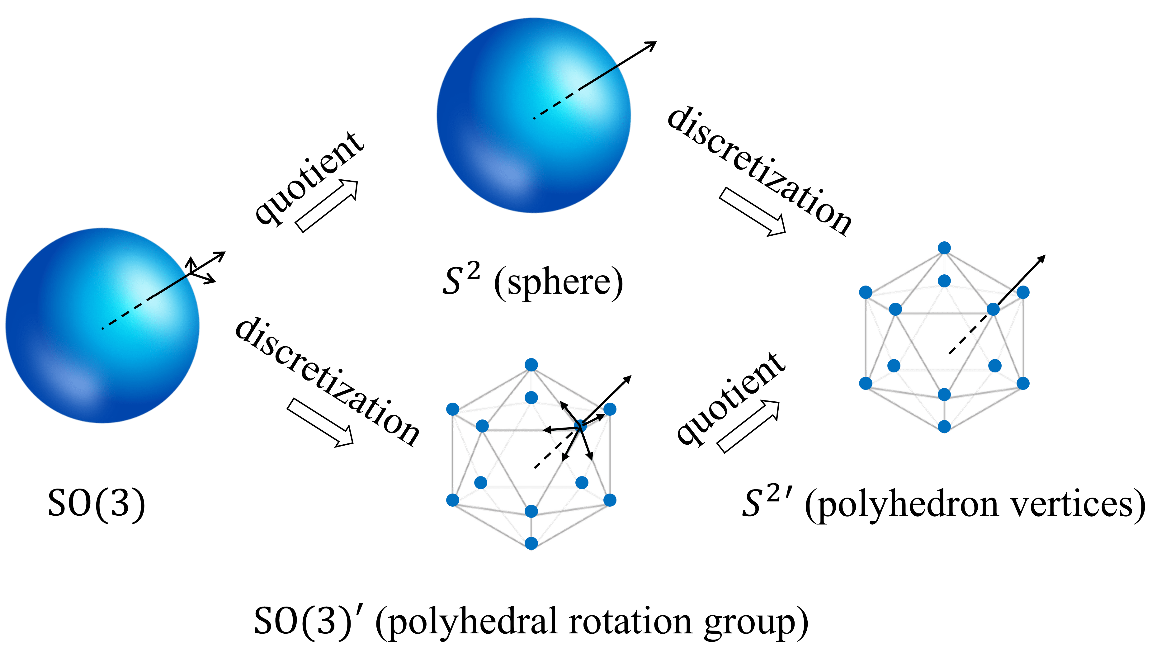
Figure 1: Our method achieves higher efficiency by working with smaller feature maps defined on $S^{2}{{}^{\prime}}\times\mathbb{R}^{3}$ rather than $SO(3)^{\prime}\times\mathbb{R}^{3}$ (^′ denotes discretization). $\mathbb{R}^{3}$ is omitted in the figure. The black arrows in each space represent elements. The top and bottom paths are equivalent, showing the relations among different representations.

A lot of progress has been made in group-equivariant feature learning. The term group encompasses the 3D rotations and translations, which is called the special Euclidean group of dimension 3, denoted $\mathrm{SE}(3)$, and also other more general types of transformations that represent certain symmetries. While many methods have been proposed, equivariant feature learning has not yet become the default strategy for 3D deep learning tasks. From our understanding, two major reasons hinder the broader application of equivariant methods. First, networks dealing with continuous groups typically require specially designed operations not commonly used in neural networks, such as generalized Fourier transform and Monte Carlo sampling. Thus, incorporating them into general neural networks for 3D learning tasks is challenging. Second, for the strategy of working on discretized (finite) groups [6, 19], while the network structures are simpler and closer to conventional networks, they usually suffer from the high dimensionality of the feature maps and convolutions, which causes much larger memory usage and computational load, limiting their practical use.

This work proposes E2PN, a convolution structure for processing 3D point clouds. Our proposed approach can enable $\mathrm{SE}(3)$-equivariance on any network with the KPConv [35] backbone by swapping KPConv with E2PN. The equivariance is up to a discretization on $\mathrm{SO}(3)$. We leverage a quotient representation to save computational and memory costs by reducing $\mathrm{SE}(3)$ feature maps to feature maps defined on $S^{2}\times\mathbb{R}^{3}$ (where $S^{2}$ stands for the 2-sphere). Nevertheless, we can recover the full 6 DoF information through a final permutation layer. As a result, our proposed network is $\mathrm{SE}(3)$-equivariant and computationally efficient, ready for practical point-cloud learning applications.

Overall, this work has the following contributions:

• We propose an efficient $\mathrm{SE}(3)$-equivariant convolution structure for 3D point clouds.

• We design a permutation layer to recover the full $\mathrm{SE}(3)$ information from its quotient space.

• We achieve comparable or better performance with significantly reduced computational cost than existing equivariant models.

• Our implementation is open-sourced at https://github.com/minghanz/E2PN.

Readers can find preliminary introductions to some related background concepts in the appendix.

2 Related work

Group convolutions: In 2016, Cohen and Welling proposed G-CNN [6], enabling equivariance beyond translations on 2D images with generalized G-convolutions (group convolutions) over the group of 90-degree rotations, which is one of the earliest efforts in equivariant deep learning. Group convolution is similar to conventional convolutions but has an extended domain for feature maps and kernels. The idea was then applied to different networks to enable equivariance for $\mathrm{SE}(2)$ [6, 19], $\mathrm{SO}(3)$ [5], $\mathrm{SE}(3)$ [42, 2], and $\mathrm{E}(3)$ [41] groups up to some discretization. The idea mainly works with finite (discretized) groups, as it is convenient to parameterize feature maps and kernels on the discretized group elements just as on pixel grids. Group convolutions have a relatively simple structure, making them straightforward to apply, but a major downside is that the lifted domain of features and kernels causes higher computational and memory costs, and the problem is more prominent when the group is large. Groups convs can also work with continuous groups, for example, with the help of Monte Carlo (MC) estimation as in [13], but they suffer from a large memory burden in MC sampling when the number of layers grows [30].

Steerable CNNs: Another line of work is steerable CNNs. Instead of augmenting the domain of feature maps, steerable CNNs generalize the space of feature values to be steerable, i.e., the feature values transform predictably as the input transforms. The way the feature transforms is called the group representation in the feature space, governed by the feature type. Features of scalar type are kept unchanged under group actions, and we call the group representation trivial. For vector or tensor feature types, the representation is not trivial, and the features will change with group actions, for example, through rotation matrix multiplication. Steerable CNNs work for both discretized and continuous groups. One may freely design the feature types based on pre-determined basic types and corresponding representations (irreducible representations, i.e., irreps) as building blocks for a given group. Group convolutions can be viewed as a special case of steerable CNNs with regular representations, i.e., channels of a feature vector undergo permutations when transformed. Examples of steerable CNNs include [9, 4, 43, 40, 36]. While the framework of steerable CNNs generalizes group convolutions with more flexibility, it requires a good understanding of representation theory and involves generalized Fourier analysis when working with a continuous group, which makes the structure complicated and challenging to apply in real-world applications broadly. The work of [39, 21] also found empirically that steerable CNNs with irreps underperform regular representations in certain tasks.

Theoretical progress: There has been a lot of progress in the theoretical development of equivariant networks that are not group-specific. [24] developed a general formulation for steerable CNNs with scalar type features, and [8, 7] generalized it to arbitrary feature types. It is proven that all equivariant linear maps can be written as convolutions. The formulation from the perspective of Fourier analysis was presented in [46]. [39] found the general form of solution for the equivariant kernels for $E(2)$ group, later generalized to any compact group [26]. [14] proposed an algorithm to solve for the equivariance constraint for arbitrary matrix group. The formulation of group convolution based on MC estimation was proposed for any Lie group with [13] or without [30] surjective exponential maps. Equivariant non-linear layers like transformers [21, 15] and equivariant set and graph networks [14, 32, 22] are also proposed, but they are not the focus of this paper.

Applications of equivariant learning in perception tasks: We want to highlight a few equivariant networks that gain attention in perception applications due to their simplicity and practicality. Vector Neurons [10] is a PointNet-like $\mathrm{SO}(3)$-equivariant network for 3D point cloud learning, later applied to point cloud registration [49] and manipulation [34]. It can be viewed as a special case of TFN [36] with type-1 features and self-interactions only. E2CNN [39] as an $\mathrm{SE}(2)$-equivariant framework was applied in several image processing tasks [33, 27], given its generality and user-friendly library. DEVIANT [25] applied scale-equivariant convolutions in monocular 3D object detection. EPN [2] is a group convolution network with $\mathrm{SE}(3)$-equivariance for 3D point cloud learning based on KPConv [35] and was used in practice, for example in place recognition task [29]. We also position this proposed work in this category, aiming to promote the application of equivariant learning with our efficient and easy-to-use design. Our work is developed based on EPN, which also serves as a major baseline in this paper.

3 Methodology

3.1 Overview of the idea

We first explain why our proposed method is more efficient. Then we discuss how we gain efficiency without sacrificing expressiveness.

3.1.1 Improved efficiency with quotient features

Following the idea of group convolutions, one needs to extend the domain of feature maps from the Euclidean space to the group space, from $\mathbb{R}^{3}$ to $\mathrm{SE}(3)\cong\mathrm{SO}(3)\times\mathbb{R}^{3}$ in our case, where we want $\mathrm{SE}(3)$-equivariant features for 3D point clouds. We then discretize $\mathrm{SO}(3)$ to a finite group denoted as $\mathrm{SO}(3)^{\prime}$ (we use ^′ to denote discretization in this paper). The discretization of $\mathbb{R}^{3}$ is taken care of by KPConv, which is the non-equivariant counterpart of our method, thus, not discussed here. Up to now, we can obtain a $\mathrm{SE}(3)$-equivariant version of KPConv [35] realized through group convolution, which is what EPN [2] presents.

The specific form of the finite group $\mathrm{SO}(3)^{\prime}$ is introduced later in Sec. 3.2, but it can be geometrically understood as the set of all rotations that keep a Platonic solid (i.e., a convex and regular 3D polyhedron) unchanged. As illustrated at the bottom of Fig. 1, the set of rotations can be enumerated by counting the number of vertices, representing rotations taking a given vertex to any vertices, multiplied by the number of edges connected to a single vertex, representing the rotations that keep a vertex fixed. The same result can be achieved by counting the faces or the edges, but we stick with vertices in the following discussion.

In comparison, we propose to define feature maps on $S^{2}\times\mathbb{R}^{3}$, where $S^{2}$ is the sphere space. We have $S^{2}=\mathrm{SO}(3)/\mathrm{SO}(2)$, meaning that it is the quotient space of $\mathrm{SO}(3)$ given the stabilizer subgroup $\mathrm{SO}(2)$. To understand the quotient space intuitively, we can see that all rotations can be grouped by the destination of a point on the sphere (e.g., the north pole) after the rotation. All rotations bringing the north pole to the same destination point form a coset. They are related by rotations around the axis passing through that point, forming a subgroup isomorphic to $\mathrm{SO}(2)$. Thus $S^{2}$ is the quotient of $\mathrm{SO}(3)$ and $\mathrm{SO}(2)$. In the discretized setup, as depicted in Fig. 1, $\mathrm{SO}(2)^{\prime}$ is discretized by the number of edges connected to a single vertex. The quotient $S^{2}{{}^{\prime}}=\mathrm{SO}(3)^{\prime}/\mathrm{SO}(2)^{\prime}$ corresponds to the vertices on the Platonic solid.

In general, $|S^{2}{{}^{\prime}}|=|\mathrm{SO}(3)^{\prime}|/|\mathrm{SO}(2)^{\prime}|<|\mathrm{SO}(3)^{\prime}|$, thus the size of feature maps and kernels defined on $S^{2}{{}^{\prime}}\times\mathbb{R}^{3}$ is much smaller than those on $\mathrm{SO}(3)^{\prime}\times\mathbb{R}^{3}$. The convolution operation on the former space also requires smaller costs. It is the major reason our method is much more efficient than EPN. There is another design, called symmetric kernel, which further improves the efficiency of our method, but we will refer to Sec. 3.2.3 for details.

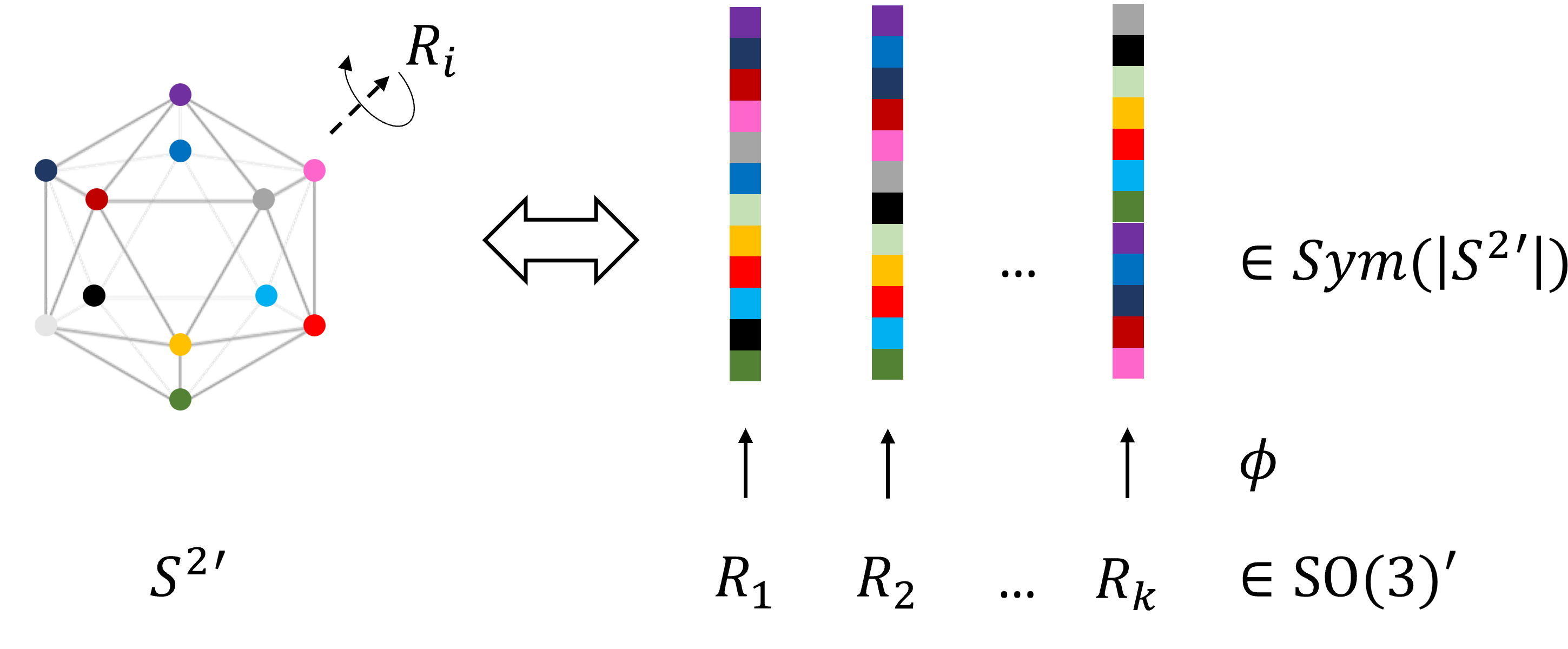
Figure 2: Illustration of recovering $\mathrm{SO}(3)^{\prime}$ features from $S^{2}{{}^{\prime}}$ features through permutations. The left and right subplots are from the geometric and algebraic views. See Sec. 3.1.2 for more explanation.

3.1.2 Information recovery with permutations

With the quotient feature map, all rotations moving the north pole to the same point on a sphere are represented by the same point. Thus we immediately lose the ability to distinguish among these rotations, which is a problem if our task is to learn the pose, for example, in the point cloud registration tasks.

However, with our proposed permutation layer, we can distinguish every element in $\mathrm{SO}(3)^{\prime}$ from the feature maps on $S^{2}{{}^{\prime}}$. The key observation is that the action of $\mathrm{SO}(3)$ on $S^{2}$ is faithful, i.e., $\forall R\in\mathrm{SO}(3)$ and $R\neq I$, $\exists x\in S^{2}$, s.t. $Rx\neq x$. It means that an action of $\mathrm{SO}(3)$ other than identity will always cause a change on the $S^{2}$ feature map when looking at all points on $S^{2}$ simultaneously. In the discretized setup, it means that there is an injective map $\phi:\mathrm{SO}(3)^{\prime}\rightarrow Sym(|S^{2}{{}^{\prime}}|)$, where $Sym(|S^{2}{{}^{\prime}}|)$ stands for the symmetric group, i.e., the collection of all permutations of a set of size $|S^{2}{{}^{\prime}}|$. An element in $Sym(n)$ is a bijective map $\{1,...,n\}\rightarrow\{1,...,n\}$, permuting the indices. In other words, each rotation corresponds to a unique permutation of the $S^{2}{{}^{\prime}}$ elements, from which we can distinguish each rotation from the feature map defined on $S^{2}{{}^{\prime}}$.

Here we provide the specific form of the permutation layer. Given $\phi$ mentioned above and a feature map $f:S^{2}{{}^{\prime}}\rightarrow\mathbb{R}^{m}$, we can build a feature map $\tilde{f}:\mathrm{SO}(3)^{\prime}\rightarrow\mathbb{R}^{mn}$ defined as:

$$\tilde{f}(R)=[f(x[\phi_{R}(1)]),f(x[\phi_{R}(2)]),...,f(x[\phi_{R}(n)])]$$ (1)

where $R\in\mathrm{SO}(3)^{\prime}$, $n=|S^{2}{{}^{\prime}}|$, and $x[i]\in S^{2}{{}^{\prime}}$ for $i=1,...,n$. Given that $\phi$ is injective, $\tilde{f}(R_{1})\neq\tilde{f}(R_{2})$ when $R_{1}\neq R_{2}$. Thus we can distinguish $\mathrm{SO}(3)^{\prime}$ rotations from $\tilde{f}$. See Fig. 2 for an illustration.

3.2 Specific form of convolution

3.2.1 Recap of KPConv

A conventional 3D convolution can be written as:

$$[\kappa*f](x)=\int_{\mathbb{R}^{3}}\kappa(t)f(x+t)\text{d}t=\sum_{t\in\mathbb{R}^{3}{{}^{\prime}}}\kappa(t)f(x+t),$$ (2)

where $x\in\mathbb{R}^{3}$, and the right hand side is after discretization. We use correlations to implement convolutions in this paper following conventions in deep learning. For processing point clouds, Eq. 2 could be tricky in implementation because it is challenging to align $\kappa$ with $f$ when there is no grid. The strategy of KPConv is to have a set of kernel points for $\kappa$ and to gather features to the kernel point coordinates from the input points where $f$ is defined so that they are aligned before the convolution. It is depicted in Fig. 3 (a), and we need to replace $f$ with $\hat{f}$ in Eq. 2 where $\hat{f}(x)=\sum_{y\in\mathcal{N}_{x}}w(|y-x|)f(y)$ and $w$ is a scalar weight function based on distance. $\hat{f}$ is the features gathered from neighboring input points to align with the kernel points. In this case, the input and output feature map $f$ and $[\kappa*f]$ are defined on $\mathbb{R}^{3}$, while the kernel $\kappa$ is defined on $\mathbb{R}^{3}{{}^{\prime}}$, i.e., coordinates of the set of kernel points. The gathered feature $\hat{f}$ when calculating the convolution at $x\in\mathbb{R}^{3}$ is defined at $x+\mathbb{R}^{3}{{}^{\prime}}$. Notice that we do not consider the deformable mode of KPConv in this paper.

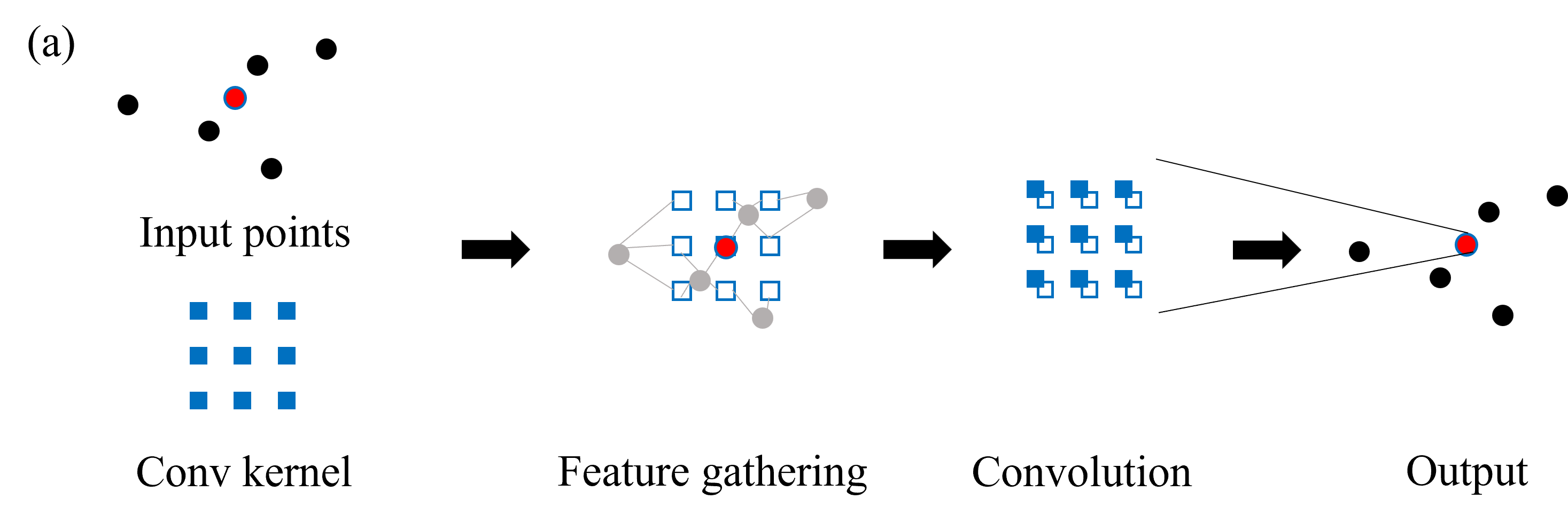
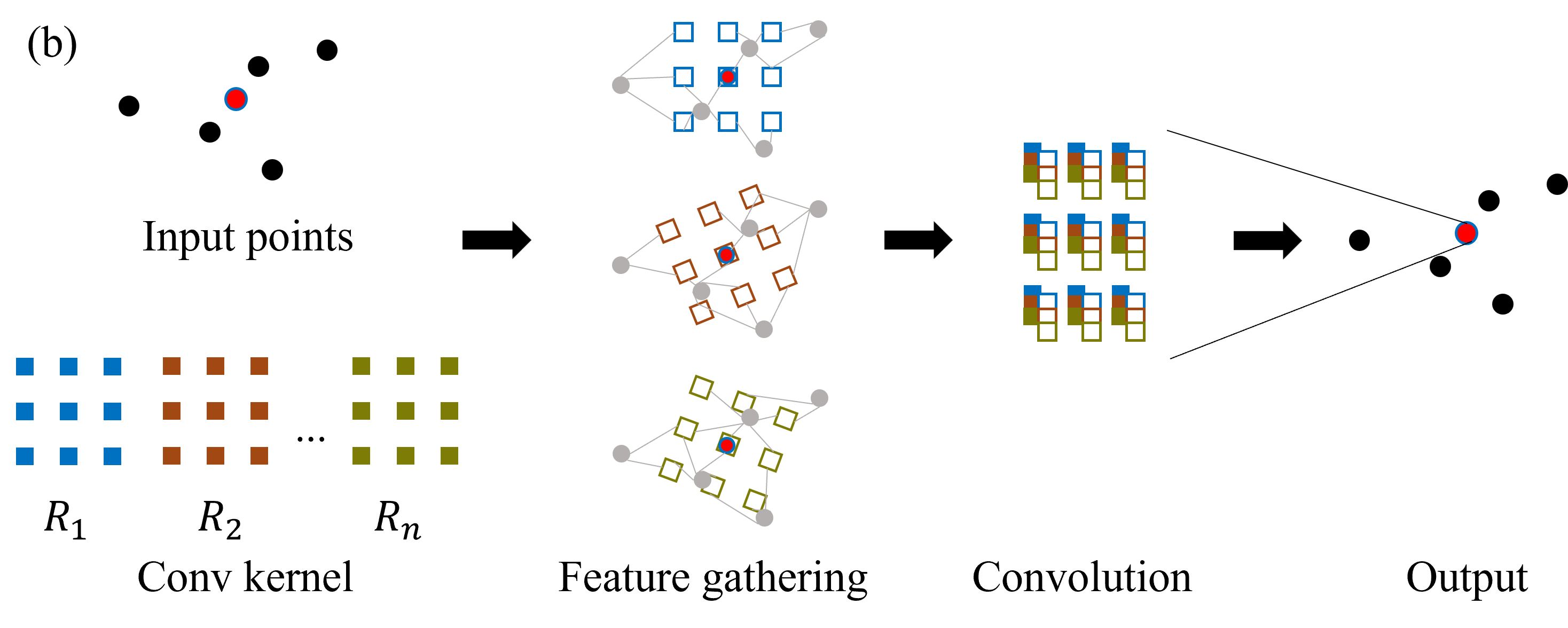
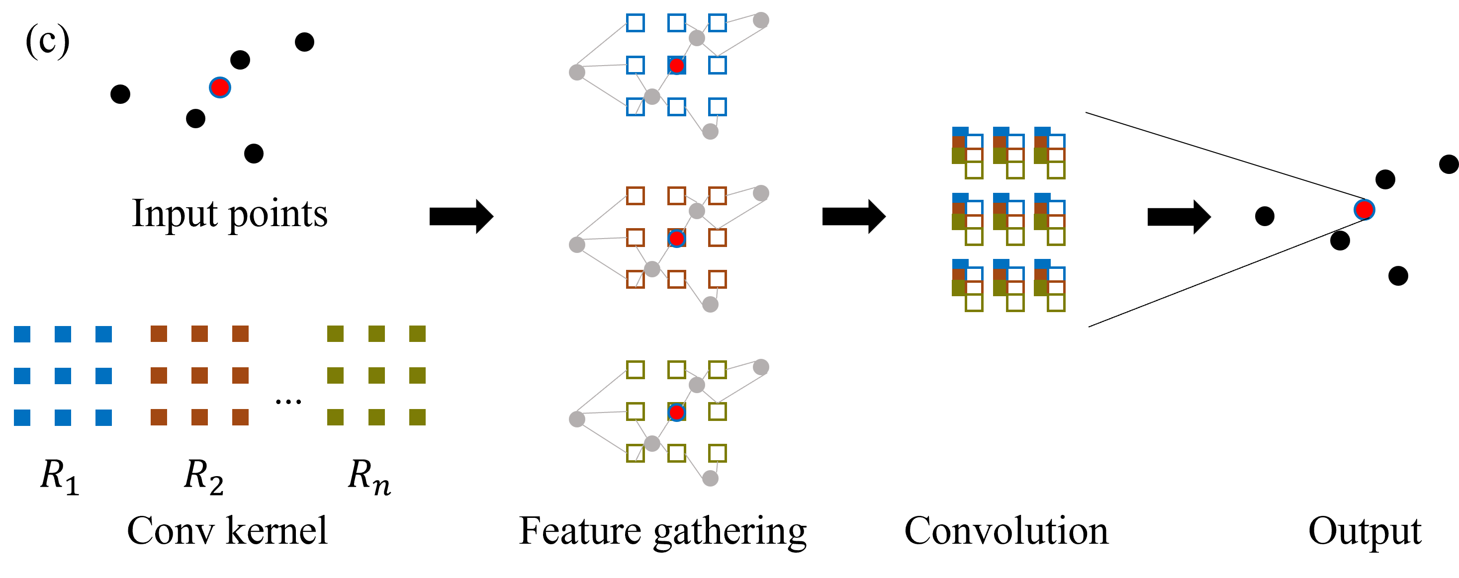
Figure 3: Illustration of different versions of KPConv. (a) original KPConv (see Sec. 3.2.1). (b) KPConv on finite group or quotient space without the symmetric kernel (see Sec. 3.2.2). (c) KPConv on group or quotient space with the symmetric kernel (see Sec. 3.2.3). (b,c) compared with (a): the convolution kernel is larger because it is defined on a higher dimension. (c) compared with (b): the feature gathering is more efficient because the kernel points are symmetric to the rotations in the rotation group.

3.2.2 KPConv on group and on quotient space

To extend KPConv to a group convolution [6] with finite group $G^{\prime}$, we modify Eq. 2 to

$$[\kappa*f](g)=\sum_{g_{t}\in G^{\prime}}\kappa(g_{t})\hat{f}(g\cdot g_{t}),$$ (3)

where in our case, $G^{\prime}=\mathrm{SE}(3)^{\prime}=\mathrm{SO}(3)^{\prime}\times\mathbb{R}^{3}{{}^{\prime}}$ is where $\kappa$ is defined, $g\in G^{\dagger}=\mathrm{SO}(3)^{\prime}\times\mathbb{R}^{3}$ is where the input and output feature map is defined. $\hat{f}$ is defined on $g\cdot G^{\prime}$ when calculating the convolution at $g$. Denote an element $g\in\mathrm{SE}(3)$ as $(R,t)$ where $R\in\mathrm{SO}(3)$ and $t\in\mathbb{R}^{3}$, the binary operation $\cdot$ for $\mathrm{SE}(3)$ can be specified as $(R_{1},t_{1})\cdot(R_{2},t_{2})=(R_{1}R_{2},t_{1}+R_{1}t_{2})$, same for the discretized case. EPN [2] follows this form of convolution. However, as discussed in Sec. 3.1.1, the size of group $|\mathrm{SE}(3)^{\prime}|=|\mathrm{SO}(3)^{\prime}||\mathbb{R}^{3}{{}^{\prime}}|$, making it expensive to store the feature map and compute the convolution. To alleviate this issue, EPN has to conduct convolutions in $\mathrm{SO}(3)^{\prime}$ and $\mathbb{R}^{3}{{}^{\prime}}$ separately (i.e., separable convolutions [2, 3]), so that the computational cost is reduced.

We use quotient feature maps to address this issue. To conduct convolutions on the quotient space $X=\mathrm{SE}(3)/\mathrm{SO}(2)=S^{2}\times\mathbb{R}^{3}$, we cannot directly use Eq. 3, because the $\cdot$ operation is not defined between two elements in $X$ since $X$ is not a group. It is pointed out in [7, 8] that we can write convolutions on the quotient space as

$$[\kappa*f](x)=\sum_{x_{t}\in X^{\prime}}\kappa(x_{t})\hat{f}(s(x)\cdot x_{t}),$$ (4)

where $X^{\prime}=S^{2}{{}^{\prime}}\times\mathbb{R}^{3}{{}^{\prime}}$ is the domain of $\kappa$, $X^{\dagger}=S^{2}{{}^{\prime}}\times\mathbb{R}^{3}$ is the domain of $f$ and $[\kappa*f]$, and $\hat{f}$ is defined on $s(x)\cdot X^{\prime}$. $s(x)$ is called the section map, $s:X^{\prime}\rightarrow G^{\prime}$ (or $X\rightarrow G$ in the continuous case), mapping $x\in X^{\prime}$ to an element of $G^{\prime}$ in the corresponding coset. With the section map, the $\cdot$ operation denotes the action of the group $G$ on quotient space $X$, i.e., $\cdot:G\times X\rightarrow X$. Denote an element in $S^{2}\times\mathbb{R}^{3}$ as $(R\mathbf{n},t)$, where $R\in\mathrm{SO}(3),\mathbf{n}$ is the north pole point on the unit sphere $(0,0,1)$. Then $R\mathbf{n}$ represents arbitrary points on the sphere $S^{2}$. The action $\cdot$ can then be written as $(R_{1},t_{1})\cdot(R_{2}\mathbf{n},t_{2})=(R_{1}R_{2}\mathbf{n},t_{1}+R_{1}t_{2})$.

3.2.3 Symmetric kernels

Now we introduce the specific form of $\mathbb{R}^{3}{{}^{\prime}}$, i.e., the location of kernel points in KPConv. In our design, $\mathbb{R}^{3}{{}^{\prime}}=\{rS^{2}{{}^{\prime}}\cup 0\mid r>0\}$ , i.e., the set of vertices of the Platonic solid with radius $r$ and the origin point. $\mathbb{R}^{3}{{}^{\prime}}$ is very similar to $S^{2}{{}^{\prime}}$, because we want to make the kernel symmetric to $\mathrm{SO}(3)^{\prime}$. More precisely, we desire $\mathbb{R}^{3}{{}^{\prime}}$ to be closed under the action of $\mathrm{SO}(3)^{\prime}$. There are two reasons as follows.

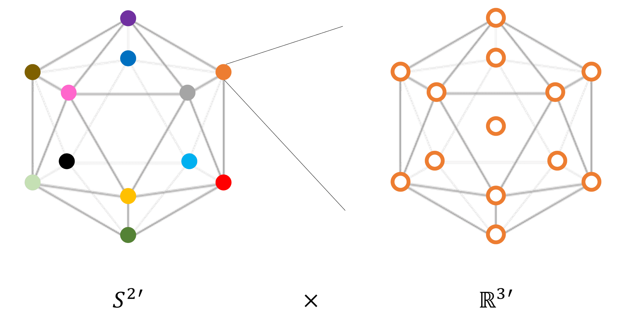
Figure 4: Visualization of the symmetric kernel $\kappa$ used in our work, where $\mathbb{R}^{3}{{}^{\prime}}=\{rS^{2}{{}^{\prime}}\cup 0\mid r>0\}$.

Steerability constraint

To make the convolution on quotient space equivariant, defining a valid form of convolution as Eq. 4 is not the whole story. The kernel values must satisfy a condition called the steerability constraint, which is required for all steerable CNNs. More background knowledge can be found in [8]. In our case, the steerability constraint is

$$\kappa(x)=\kappa(R_{z}\cdot x),\forall x\in X^{\prime},\forall R_{z}\in\mathrm{SO}(2)^{\prime},$$ (5)

where $R_{z}$ is a $z$-axis rotation. The derivation of Eq. 5 from the general form of steerability constraints can be found in the appendix. Here the $\cdot$ operation inherits from the action of $G^{\prime}$ on $X^{\prime}$ since $\mathrm{SO}(2)^{\prime}\subset\mathrm{SO}(3)^{\prime}\subset G^{\prime}$. Specifically, we have $R_{z}\cdot(R\mathbf{n},t)=(R_{z},0)\cdot(R\mathbf{n},t)=(R_{z}R\mathbf{n},R_{z}t)$. Replace $x$ with $(R\mathbf{n},t)$ in Eq. 5, and we have

$$\kappa(R\mathbf{n},t)=\kappa(R_{z}R\mathbf{n},R_{z}t),$$ (6)

$\forall R\mathbf{n}\in S^{2}{{}^{\prime}},\forall t\in\mathbb{R}^{3}{{}^{\prime}},\forall R_{z}\in\mathrm{SO}(2)^{\prime}$. Notice that it implies that we need $R_{z}t\in\mathbb{R}^{3}{{}^{\prime}},\forall t\in\mathbb{R}^{3}{{}^{\prime}},\forall R_{z}\in\mathrm{SO}(2^{\prime})$, so that $\kappa$ is defined on the right hand side of Eq. 6. In other words, the kernel points $\mathbb{R}^{3}{{}^{\prime}}$ need to be closed under $\mathrm{SO}(2)^{\prime}$. Obviously, having $\mathbb{R}^{3}{{}^{\prime}}$ closed under $\mathrm{SO}(3)^{\prime}$ is a sufficient condition for this.

For the $S^{2}{{}^{\prime}}$ dimension, since $S^{2}{{}^{\prime}}$ is symmetric (closed) to $\mathrm{SO}(3)^{\prime}$ by definition and $\mathrm{SO}(2)^{\prime}\subset\mathrm{SO}(3)^{\prime}$, we always have $R_{z}R\mathbf{n}\in S^{2}{{}^{\prime}}$ and $\kappa$ is always defined.

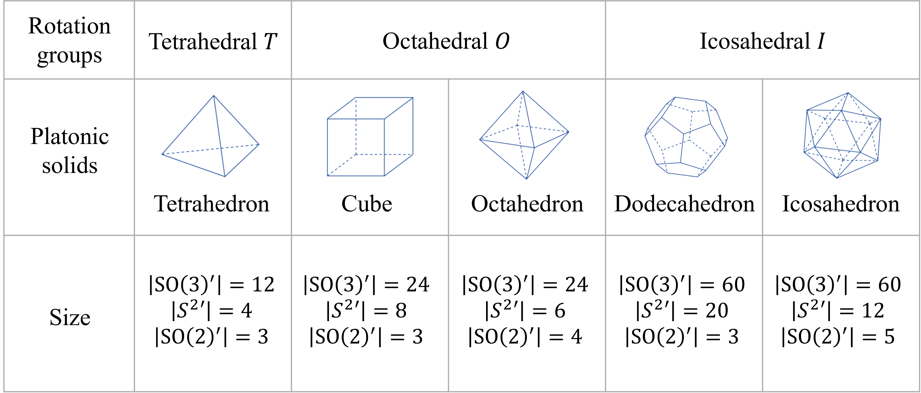
Figure 5: Illustration of all five types of Platonic solids and their corresponding finite rotation groups.

Table 1: Efficiency comparison in terms of GPU memory consumption and the computation speed between EPN [2] and our method on three tasks. Two numbers are reported for training/inference respectively. $\downarrow$ means lower is better. $\uparrow$ means higher is better. The best is shown in bold font.

Tasks ModelNet40 Pose ModelNet40 Classification 3DMatch Keypoint Matching Methods Memory (GB) $\downarrow$ Speed (fps) $\uparrow$ Memory (GB) $\downarrow$ Speed (fps) $\uparrow$ Memory (GB) $\downarrow$ Speed (fps) $\uparrow$ EPN [2] 22.2 / 16.9 1.1 / 1.6 13.4 / 12.7 1.9 / 1.5 37.4 / 8.5 0.6 / 3.1 Ours (w/o symmetric kernels) 4.8 / 3.7 5.1 / 10.1 4.1 / 3.2 7.8 / 7.8 7.5 / 2.8 2.6 / 16.7 Ours (w/ symmetric kernels) 4.3 / 2.8 6.7 / 11.1 3.9 / 2.7 9.1 / 10.3 6.5 / 2.4 3.7 / 23.6

Efficient feature gathering

Another important reason for the design choice of $\mathrm{SO}(3)^{\prime}$-symmetric kernels is that it enables more efficient feature gathering. Consider a spatial location $t_{0}\in\mathbb{R}^{3}$, the convolution feature output at this point is a stack of $[[\kappa*f](x_{i})]_{i}$ with $x_{i}\in(S^{2}{{}^{\prime}},t_{0})\subset X^{\dagger}$. As shown in Eq. 4, it involves feature gathering for $\hat{f}$ at $s(x_{i})\cdot x_{jk}$ for every $x_{jk}\in X^{\prime}=S^{2}{{}^{\prime}}\times\mathbb{R}^{3}{{}^{\prime}}$. Denote an instance of $s(x_{i})=(R_{i},t_{0}),x_{jk}=(R_{j}\mathbf{n},t_{k})$, then $s(x_{i})\cdot x_{jk}=(R_{i}R_{j}\mathbf{n},t_{0}+R_{i}t_{k})$. If $\mathbb{R}^{3}{{}^{\prime}}$ is closed under $\mathrm{SO}(3)^{\prime}$, then we have

$$\{R_{i}t_{k}|t_{k}\in\mathbb{R}^{3}{{}^{\prime}}\}=\mathbb{R}^{3}{{}^{\prime}},\forall R_{i}\in\mathrm{SO}(3)^{\prime},$$ (7)

which implies that the feature gathering for all $S^{2}{{}^{\prime}}$ channels can be done once at the same set of spatial positions specified by $\mathbb{R}^{3}{{}^{\prime}}$. An illustration is shown in Fig. 3. Without the symmetric kernel, the KPConv on group or quotient space looks like Fig. 3 (b), where the kernel is rotated for each $\mathrm{SO}(3)^{\prime}$ (for group KPConv) or $S^{2}{{}^{\prime}}$ (for quotient KPConv) channel separately to gather input features. However, with symmetric kernels, as shown in Fig. 3 (c), the rotations keep the position of kernel points unchanged up to a permutation so that the feature-gathering step is simplified. Specifically, the number of spatial positions needed for feature gathering without symmetric kernels is $|SO(3)^{\prime}||\mathbb{R}^{3}{{}^{\prime}}|$ for group KPConv or $|S^{2}{{}^{\prime}}||\mathbb{R}^{3}{{}^{\prime}}|$ for quotient KPConv, while the number is $|\mathbb{R}^{3}{{}^{\prime}}|$ with symmetric kernels. The convolution kernels in Fig. 3 is an abstract illustration, while the actual symmetric kernel in our work is visualized in Fig. 4.

3.2.4 Choices of the discretization of $SO(3)$ and $S^{2}$

In Sec. 3.1.1, we mentioned that the discretization of $\mathrm{SO}(3)$ is the rotation group that respects the symmetry of a Platonic solid. There are five types of Platonic solids, corresponding to 3 finite rotation groups, as shown in Fig. 5. Choosing $\mathrm{SO}(3)^{\prime}$ to be any of them is valid, representing a discretization of $\mathrm{SO}(3)$ to different resolutions. The different Platonic solids with the same rotation group $\mathrm{SO}(3)^{\prime}$ represents different discretizations of $S^{2}{{}^{\prime}}$ and $\mathrm{SO}(2)^{\prime}$.

If we use a small $\mathrm{SO}(3)^{\prime}$ (for example, $T$), the strategy of using $\mathbb{R}^{3}{{}^{\prime}}=\{rS^{2}{{}^{\prime}}\cup 0\mid r>0\}$ could be problematic because the number of kernel points could be too few to learn representative features. In this case, we are free to design the kernel points differently, as long as they are closed under $\mathrm{SO}(3)^{\prime}$. For example, one may add kernel points at the center of all edges and/or faces. One may even use a combination of several polyhedrons with different radii $r$.

In this paper, we only choose the icosahedron as the Platonic solid to conduct experiments for three reasons. First, it has the finest discretization of $\mathrm{SO}(3)$. Second, it has a smaller size of $S^{2}{{}^{\prime}}$ compared with the dodecahedron, maximizing the benefit of working with quotient features. Third, it is consistent with existing methods [2, 1], enabling direct comparison with the baselines.

3.2.5 Other aspects of the network

We use element-wise scalar nonlinearity (ReLu and leaky ReLu) in the network. The spatial pooling is done by subsampling the input points and aggregating the features of neighboring input points to the subsampled points. Batch normalization is applied to normalize over the batch, $S^{2}{{}^{\prime}}$, and $\mathbb{R}^{3}$ dimensions. All these choices follow the common practice of conventional CNNs (KPConv [35]) and group convolutions (EPN [2]). We also adopted the group attentive pooling in EPN to pool over the $S^{2}{{}^{\prime}}$ dimension and generate $\mathrm{SO}(3)^{\prime}$-invariant features.

Depending on the specific task in the experiment, the prediction head has a slightly different design, composing the last few layers of the network. The loss functions are inherited from EPN [2], including cross-entropy loss for classifications, L2 loss for residual pose regression, and batch-hard triplet loss for keypoint matching. We refer to the appendix for more details about the prediction heads and the loss functions.

3.3 Relation to existing work

In the context of literature on group-equivariant neural networks, our method is under the theoretical framework of equivarant CNNs on homogeneous spaces [8, 24, 46]. Our work is a new form of realization when working with 3D point clouds and adapting the convolution structure of KPConv. We explore a balance of simplicity, efficiency, and expressiveness by finding the proper quotient space and discretization. Our method is an extension of group convolutions, leveraging their clean structure enabled by discretization. Our method can also be viewed as a steerable CNN with homogeneous space $S^{2}\times\mathbb{R}^{3}$ and stabilizer subgroup $\mathrm{SO}(2)$ with scalar-type features or with homogeneous space $\mathbb{R}^{3}$ and stabilizer subgroup $\mathrm{SO}(3)$ with $S^{2}$ features. The proposed work paves the way for efficiency improvement using quotient representation learning on finite groups. We also emphasize the group-variant side of equivariant models with the permutation layer to distinguish rotations, while existing work focuses on the benefit of getting group-invariant features from equivariant models.

4 Experiments

Our major baseline to compare with is EPN [2], a state-of-the-art group convolution network, as we are similar in several ways. Both are KPConv-style convolutions with $\mathrm{SE}(3)$-equivariance. Both use the icosahedral rotation group $\mathcal{I}$ to discretize $\mathrm{SO}(3)$. However, EPN has features defined on $\mathcal{I}\times\mathbb{R}^{3}$, compared with $S^{2}{{}^{\prime}}\times\mathbb{R}^{3}$ in our method.

Two datasets, ModelNet40 [44] and 3DMatch [47], are used in the experiments. ModelNet40 is composed of 3D CAD models of 40 categories of objects. 3DMatch is a real-scan dataset of indoor scenes. For the ModelNet40 dataset, we conduct the classification and pose estimation tasks. For the 3DMatch dataset, we conduct the keypoint matching task. These tasks are also studied in EPN [2].

In Tab. 1, we list the GPU memory consumption and running speed of our method and EPN [2] in the three tasks. The comparisons are under the same input size, number of feature channels, and number of network layers. The separable convolutions on $\mathrm{SO}(3)$ and $\mathbb{R}^{3}$ in EPN are together considered as one layer. The numbers are not comparable between training and inference because the batch size could be different (see the appendix). The specific configurations in each experiment are introduced later. All experiments are run on a single NVIDIA A40 GPU. Our network with quotient space convolutions is much smaller and runs much faster in all three tasks, indicating the potential value for real applications. We boost efficiency without sacrificing performance, as is shown later.

Ablation study: We list two rows of our results in Tab. 1 to show the effect of efficient feature gathering enabled by the symmetric kernels. The results of without symmetric kernels are generated using the same kernel points as with symmetric kernels, but ignoring the fact that they are symmetric to rotations and gathering features at $|S^{2}{{}^{\prime}}||\mathbb{R}^{3}{{}^{\prime}}|$ locations, instead of at $|\mathbb{R}^{3}{{}^{\prime}}|$ locations and permuting them. The efficient feature gathering brings further efficiency improvements, especially in terms of computational speed.

Table 2: Experimental result of object classification on ModelNet40. The best is bolded. The best in equivariant models is underlined. Noisy: test using input with random translation, scaling, jittering, and dropout. Clean: test without above processing. SO(3): random rotations. Id: no rotation. ico: random rotations in $\mathcal{I}$. ESCNN works with voxelized data, thus not having Noisy results with point-wise augmentations. FLOPs are counted using fvcore, which does not support DGL used in TFN and SE(3)-T, thus left blank. The efficiency comparison uses the same batch size as in Tab. 1 (see appendix).

Type	Column #	#1	#2	#3	#4	#5	#6	#7	#8	#9	#10	#11	#12	#13	#14
	Metrics	ModelNet40 classification performance metric: Acc (%) $\uparrow$										Efficiency metrics		FLOPs per training batch (G)	Trainable params (M)
	Train rotation	SO(3)				Id						Memory (GB)$\downarrow$ train/test	Speed (fps)$\uparrow$ train/test
	Test rotation	SO(3)		Id		SO(3)		Id		ico
	Test condition	Noisy	Clean	Noisy	Clean	Noisy	Clean	Noisy	Clean	Noisy	Clean
Non-equiv	KPConv [35]	75.71	81.17	76.88	82.02	12.66	12.22	89.46	91.85	-	-	0.18/0.25	17.24/18.48	0.74	1.69
	PointNet++ [31]	81.31	84.88	83.03	85.76	13.44	13.76	90.67	91.55	-	-	1.03/0.5	7.06/7.43	10.59	1.48
	DGCNN [38]	79.86	84.77	82.54	85.62	15.36	17.26	91.00	92.18	-	-	1.96/1.69	17.90/17.50	32.65	1.81
	PT[48]	78.51	79.68	78.83	79.68	16.53	16.77	86.98	88.10	-	-	4.16/5.82	4.80/5.03	220.99	9.58
	CurveNet[45]	84.72	88.33	85.82	88.94	17.34	18.03	91.53	92.63	-	-	1.20/0.33	5.61/7.54	4.22	2.14
	PCT[17]	86.91	89.10	87.64	89.83	16.33	17.95	91.69	92.87	-	-	1.18/0.80	8.54/20.85	27.41	2.87
Equivariant	ESCNN [1]	-	82.40	-	77.73	-	29.03	-	88.94	-	-	4.71/5.50	3.79/8.38	428.61	0.46
	TFN [36]	58.27	62.64	58.06	62.64	57.50	62.28	59.20	62.28	-	-	15.95/8.7	1.83/6.08	-	0.06
	SE(3)-T [15]	60.37	66.29	61.18	66.29	44.61	50.53	44.81	50.53	-	-	19.39/9.65	1.54/5.13	-	0.11
	EPN [2]	84.63	87.84	85.34	88.83	30.99	32.32	90.03	91.61	90.04	91.60	13.40/12.72	1.86/1.49	58.95	3.06
	Ours (w/ GA pooling [2])	85.04	87.51	85.49	87.63	41.46	44.43	89.73	90.50	90.00	90.50	3.95/2.70	9.21/10.37	170.68	2.53
	Ours (w/ permutation)	86.99	88.62	88.21	89.62	39.54	42.78	90.66	91.77	90.68	91.77	3.95/2.70	9.09/10.28	170.77	2.65

4.1 Object classification on ModelNet40

For this task, given a point cloud of an object, the network predicts its category. The evaluation metric is classification accuracy (Acc). In this experiment, we show an extensive efficiency comparison with more existing networks, equivariant and non-equivariant. We also examine a wide combination of input conditions in training and testing to show the effect of equivariance and robustness against input imperfections. All models are trained with data augmentation, including random translation, scaling, jittering, and dropout.

Our method has outstanding performance as shown in Tab. 2. In columns #1-4, all methods are trained with rotational augmentation. Our method performs the best among listed equivariant models and is on par with PCT [18] among all models. Our method is intended to work with rotational augmentations so that the equivariance gap caused by discretization can be interpolated through training. However, we still experiment with training without rotational augmentation, as shown in columns #5-10. From columns #9-10, we can verify the equivariance to the icosahedral rotation group of our model. Columns #5-6 show the effect of discretization on the continuous $\mathrm{SO}(3)$ if no interpolation is trained, in which case the performance lands between non-equivariant models and continuously $\mathrm{SO}(3)$-equivariant models. The efficiency of our method outperforms all equivariant baselines and is similar to non-equivariant models. The FLOPs and number of trainable parameters are also listed for reference. We found that FLOPs do not strictly correlate with running speed, which could be due to different memory access costs and parallelism.

Table 3: Pose estimation on ModelNet40. Mean, median, and max angular errors are calculated over the test set. Statistics (average and standard deviation) over 10 test runs are shown to account for the randomness.

Metrics Mean ($\degree$) $\downarrow$ Median ($\degree$) $\downarrow$ Max ($\degree$) $\downarrow$ Stats Avg $\mu$ SD $\sigma$ Avg $\mu$ SD $\sigma$ Avg $\mu$ SD $\sigma$ KPConv [35] 13.99 1.53 10.70 0.81 115.19 57.84 EPN [2] 1.10 0.20 1.36 0.13 7.06 2.52 Ours 1.20 0.08 0.96 0.05 6.71 1.28

Ablation study: Since this task requires $\mathrm{SE}(3)$-invariant features, there are two options in our network: either using the group-attentive pooling (GA pooling) introduced in EPN [2] to pool over the $S^{2}{{}^{\prime}}$ dimensions or using the permutation layer to find the canonical permutation of $S^{2}{{}^{\prime}}$ dimensions. Either way, the canonical pose of objects in ModelNet40 can be used for supervision. Tab. 2 shows that the permutation layer yields better performance with negligible computational overhead. The reason could be that the permutation layer as in Eq. 1 stacks features from $S^{2}{{}^{\prime}}$ and thus preserves the information better, compared with weighted averaging over the $S^{2}{{}^{\prime}}$ dimension as done in GA pooling.

4.2 Pose Estimation on ModelNet40

In this experiment, the network takes a pair of point clouds of an object and predicts the relative rotation between them. To avoid the pose ambiguity of objects with symmetric rotational shapes, only the airplane category is used in this experiment, with 626 models in the training set and 100 models in the test set. A point cloud is generated by randomly subsampling 1,024 points on the surface, and it is randomly rotated to form a pair.

The experimental result is shown in Tab. 3. We achieved similar rotation estimation accuracy to EPN [2] overall. While our mean error is slightly larger, the lower median error, max error, and standard deviations show that our method delivers a more reliable registration. It could imply that representing rotations as a permutation of features is more robust than representing them as a single element in the feature map. Besides, the equivariant networks outperform the non-equivariant KPConv [35] by a large margin.

Table 4: Experiment result of keypoint matching on the 3DMatch dataset. The numbers are the average recall ($\%$), and the higher, the better. Notation * represents the result with the given point normal information.

SHOT[37] 3DM[47] CGF[23] PPFN[12] PPFF[11] 3DSN[16] Li[28] Li[28]* EPN[2] Ours Kitchen 74.3 58.3 60.3 89.7 78.7 97.5 92.1 99.4 99.0 99.4 Home 1 80.1 72.4 71.1 55.8 76.3 96.2 91.0 98.7 99.4 98.7 Home 2 70.7 61.5 56.7 59.1 61.5 93.2 85.6 94.7 96.2 96.6 Hotel 1 77.4 54.9 57.1 58.0 68.1 97.4 95.1 99.6 99.6 99.1 Hotel 2 72.1 48.1 53.8 57.7 71.2 92.8 91.3 100.0 97.1 98.1 Hotel 3 85.2 61.1 83.3 61.1 94.4 98.2 96.3 100.0 100.0 100.0 Study 64.0 51.7 37.7 53.4 62.0 95.0 91.8 95.5 96.2 95.2 MIT Lab 62.3 50.7 45.5 63.6 62.3 94.1 84.4 92.2 93.5 90.9 Average 73.3 57.3 58.2 62.3 71.8 95.6 91.0 97.5 97.6 97.3

4.3 Keypoint matching on 3DMatch

In this task, patches of point clouds extracted locally around keypoints in a large, dense scan are input to the network, and each is mapped to a feature vector of 64-dimension as the keypoint descriptor. Each patch has 1,024 points. Then we evaluate the average recall of keypoint correspondence across different scans through nearest neighbor search in the feature space, as proposed in PPFNet [12].

This experiment’s performance in Tab. 4 indicates the capability of learning distinctive and rotation-invariant features for local patches of point clouds. Though not achieving the best in the list, our method delivers comparable performance to the top methods using only a fraction of the computational resources as EPN [2] (see Tab. 1). We use the GA pooling layer [2] in this experiment because the permutation layer requires supervision on the pose, while a canonical pose is not defined for local patches of point clouds, and GA pooling works with or without the pose supervision. However, the result shows that GA pooling over the $\left\lvert S^{2}{{}^{\prime}}\right\rvert$ features also provides distinctive features for keypoint matching. This part may be further improved by taking the information of the global scan [12] or the matching scan [20] into consideration, in which case the permutation layer may get hints on the optimal permutation from the larger context. This topic goes beyond the focus of this paper and is left for future work.

5 Conclusion

This paper presents a new design of $\mathrm{SE}(3)$-equivariant point cloud convolution network, which is efficient, simple, and expressive simultaneously by working with feature maps defined on the quotient space $S^{2}\times\mathbb{R}^{3}$ associated with the stabilizer $\mathrm{SO}(2)$. We further improve the efficiency of the convolutions by designing the kernel points to be symmetric to the discretized rotation group $\mathrm{SO}(3)^{\prime}$. Moreover, we propose a permutation layer to recover $\mathrm{SO}(3)^{\prime}$ information from $S^{2}{{}^{\prime}}$ dimensions of the features so that the network can detect $\mathrm{SO}(3)$ rotations. Experiments show that our network delivers state-of-the-art performance in multiple tasks while consuming only a fraction of memory and computation resources as a group-convolution network with similar performance. Our method can open exciting opportunities to introduce the $\mathrm{SE}(3)$-equivariance property to mainstream point cloud networks for various tasks.

This work also has limitations. We do not outperform EPN [2] in the keypoint matching task, implying that the network, especially the permutation layer, needs improvement when dealing with inputs without a clear pose definition. Other possibilities for the network design also remain open. For example: What if we use a non-scalar type of feature on the quotient space? How to further alleviate the impact of the discretization of a continuous group? From a general perspective, extending the discretized quotient space convolution strategy to other groups is also an attractive direction for future work.

References

- [1] Gabriele Cesa, Leon Lang, and Maurice Weiler. A program to build E(N)-equivariant steerable CNNs. In International Conference on Learning Representations, 2022.
- [2] Haiwei Chen, Shichen Liu, Weikai Chen, Hao Li, and Randall Hill. Equivariant point network for 3D point cloud analysis. In Proceedings of the IEEE Conference on Computer Vision and Pattern Recognition, pages 14514–14523, 2021.
- [3] François Chollet. Xception: Deep learning with depthwise separable convolutions. In Proceedings of the IEEE conference on computer vision and pattern recognition, pages 1251–1258, 2017.
- [4] Taco Cohen, Mario Geiger, Jonas Köhler, and Max Welling. Convolutional networks for spherical signals. arXiv preprint arXiv:1709.04893, 2017.
- [5] Taco Cohen, Maurice Weiler, Berkay Kicanaoglu, and Max Welling. Gauge equivariant convolutional networks and the icosahedral CNN. In International conference on Machine learning, pages 1321–1330. PMLR, 2019.
- [6] Taco Cohen and Max Welling. Group equivariant convolutional networks. In International conference on machine learning, pages 2990–2999. PMLR, 2016.
- [7] Taco S Cohen, Mario Geiger, and Maurice Weiler. Intertwiners between induced representations (with applications to the theory of equivariant neural networks). arXiv preprint arXiv:1803.10743, 2018.
- [8] Taco S Cohen, Mario Geiger, and Maurice Weiler. A general theory of equivariant CNNs on homogeneous spaces. Proceedings of the Advances in Neural Information Processing Systems Conference, 32, 2019.
- [9] Taco S Cohen and Max Welling. Steerable cnns. arXiv preprint arXiv:1612.08498, 2016.
- [10] Congyue Deng, Or Litany, Yueqi Duan, Adrien Poulenard, Andrea Tagliasacchi, and Leonidas J Guibas. Vector Neurons: A general framework for SO(3)-equivariant networks. In Proceedings of the IEEE International Conference on Computer Vision, pages 12200–12209, 2021.
- [11] Haowen Deng, Tolga Birdal, and Slobodan Ilic. PPF-FoldNet: Unsupervised learning of rotation invariant 3D local descriptors. In Proceedings of the European Conference on Computer Vision, pages 602–618, 2018.
- [12] Haowen Deng, Tolga Birdal, and Slobodan Ilic. PPFNet: Global context aware local features for robust 3D point matching. In Proceedings of the IEEE Conference on Computer Vision and Pattern Recognition, pages 195–205, 2018.
- [13] Marc Finzi, Samuel Stanton, Pavel Izmailov, and Andrew Gordon Wilson. Generalizing convolutional neural networks for equivariance to lie groups on arbitrary continuous data. In International Conference on Machine Learning, pages 3165–3176. PMLR, 2020.
- [14] Marc Finzi, Max Welling, and Andrew Gordon Wilson. A practical method for constructing equivariant multilayer perceptrons for arbitrary matrix groups. In International Conference on Machine Learning, pages 3318–3328. PMLR, 2021.
- [15] Fabian Fuchs, Daniel Worrall, Volker Fischer, and Max Welling. SE(3)-transformers: 3D roto-translation equivariant attention networks. Proceedings of the Advances in Neural Information Processing Systems Conference, 33:1970–1981, 2020.
- [16] Zan Gojcic, Caifa Zhou, Jan D Wegner, and Andreas Wieser. The perfect match: 3D point cloud matching with smoothed densities. In Proceedings of the IEEE Conference on Computer Vision and Pattern Recognition, pages 5545–5554, 2019.
- [17] Meng-Hao Guo, Jun-Xiong Cai, Zheng-Ning Liu, Tai-Jiang Mu, Ralph R Martin, and Shi-Min Hu. Pct: Point cloud transformer. Computational Visual Media, 7:187–199, 2021.
- [18] Meng-Hao Guo et al. Pct: Point cloud transformer. Computational Visual Media, 2021.
- [19] Emiel Hoogeboom, Jorn WT Peters, Taco S Cohen, and Max Welling. HexaConv. In International Conference on Learning Representations, 2018.
- [20] Shengyu Huang, Zan Gojcic, Mikhail Usvyatsov, Andreas Wieser, and Konrad Schindler. Predator: Registration of 3D point clouds with low overlap. In Proceedings of the IEEE Conference on Computer Vision and Pattern Recognition, pages 4267–4276, 2021.
- [21] Michael J Hutchinson, Charline Le Lan, Sheheryar Zaidi, Emilien Dupont, Yee Whye Teh, and Hyunjik Kim. Lietransformer: Equivariant self-attention for lie groups. In International Conference on Machine Learning, pages 4533–4543. PMLR, 2021.
- [22] Nicolas Keriven and Gabriel Peyré. Universal invariant and equivariant graph neural networks. Proceedings of the Advances in Neural Information Processing Systems Conference, 32, 2019.
- [23] Marc Khoury, Qian-Yi Zhou, and Vladlen Koltun. Learning compact geometric features. In Proceedings of the IEEE International Conference on Computer Vision, pages 153–161, 2017.
- [24] Risi Kondor and Shubhendu Trivedi. On the generalization of equivariance and convolution in neural networks to the action of compact groups. In International Conference on Machine Learning, pages 2747–2755. PMLR, 2018.
- [25] Abhinav Kumar, Garrick Brazil, Enrique Corona, Armin Parchami, and Xiaoming Liu. Deviant: Depth equivariant network for monocular 3d object detection. In Computer Vision–ECCV 2022: 17th European Conference, Tel Aviv, Israel, October 23–27, 2022, Proceedings, Part IX, pages 664–683. Springer, 2022.
- [26] Leon Lang and Maurice Weiler. A Wigner-Eckart theorem for group equivariant convolution kernels. arXiv preprint arXiv:2010.10952, 2020.
- [27] Jongmin Lee, Byungjin Kim, and Minsu Cho. Self-supervised equivariant learning for oriented keypoint detection. In Proceedings of the IEEE Conference on Computer Vision and Pattern Recognition, pages 4847–4857, June 2022.
- [28] Lei Li, Siyu Zhu, Hongbo Fu, Ping Tan, and Chiew-Lan Tai. End-to-end learning local multi-view descriptors for 3D point clouds. In Proceedings of the IEEE Conference on Computer Vision and Pattern Recognition, pages 1919–1928, 2020.
- [29] Chien Erh Lin, Jingwei Song, Ray Zhang, Minghan Zhu, and Maani Ghaffari. Epn-netvlad: Se (3)-invariant place recognition for 3d point clouds. In 6th Annual Conference on Robot Learning.
- [30] Lachlan E MacDonald, Sameera Ramasinghe, and Simon Lucey. Enabling equivariance for arbitrary Lie groups. In Proceedings of the IEEE Conference on Computer Vision and Pattern Recognition, pages 8183–8192, 2022.
- [31] Charles Ruizhongtai Qi, Li Yi, Hao Su, and Leonidas J Guibas. PointNet++: Deep hierarchical feature learning on point sets in a metric space. Proceedings of the Advances in Neural Information Processing Systems Conference, 30, 2017.
- [32] Nimrod Segol and Yaron Lipman. On universal equivariant set networks. arXiv preprint arXiv:1910.02421, 2019.
- [33] Ahyun Seo, Byungjin Kim, Suha Kwak, and Minsu Cho. Reflection and rotation symmetry detection via equivariant learning. In Proceedings of the IEEE Conference on Computer Vision and Pattern Recognition, pages 9539–9548, June 2022.
- [34] Anthony Simeonov, Yilun Du, Andrea Tagliasacchi, Joshua B Tenenbaum, Alberto Rodriguez, Pulkit Agrawal, and Vincent Sitzmann. Neural Descriptor Fields: SE(3)-equivariant object representations for manipulation. In Proceedings of the IEEE International Conference on Robotics and Automation, pages 6394–6400. IEEE, 2022.
- [35] Hugues Thomas, Charles R. Qi, Jean-Emmanuel Deschaud, Beatriz Marcotegui, François Goulette, and Leonidas J. Guibas. Kpconv: Flexible and deformable convolution for point clouds. Proceedings of the IEEE International Conference on Computer Vision, 2019.
- [36] Nathaniel Thomas, Tess Smidt, Steven Kearnes, Lusann Yang, Li Li, Kai Kohlhoff, and Patrick Riley. Tensor field networks: Rotation-and translation-equivariant neural networks for 3d point clouds. arXiv preprint arXiv:1802.08219, 2018.
- [37] Federico Tombari, Samuele Salti, and Luigi Di Stefano. Unique shape context for 3d data description. In Proceedings of the ACM workshop on 3D object retrieval, pages 57–62, 2010.
- [38] Yue Wang, Yongbin Sun, Ziwei Liu, Sanjay E Sarma, Michael M Bronstein, and Justin M Solomon. Dynamic graph cnn for learning on point clouds. Acm Transactions On Graphics (TOG), 38(5):1–12, 2019.
- [39] Maurice Weiler and Gabriele Cesa. General E(2)-equivariant steerable CNNs. Proceedings of the Advances in Neural Information Processing Systems Conference, 32, 2019.
- [40] Maurice Weiler, Mario Geiger, Max Welling, Wouter Boomsma, and Taco S Cohen. 3D steerable CNNs: Learning rotationally equivariant features in volumetric data. Proceedings of the Advances in Neural Information Processing Systems Conference, 31, 2018.
- [41] Marysia Winkels and Taco S Cohen. 3D G-CNNs for pulmonary nodule detection. arXiv preprint arXiv:1804.04656, 2018.
- [42] Daniel Worrall and Gabriel Brostow. CubeNet: Equivariance to 3D rotation and translation. In Proceedings of the European Conference on Computer Vision, pages 567–584, 2018.
- [43] Daniel E Worrall, Stephan J Garbin, Daniyar Turmukhambetov, and Gabriel J Brostow. Harmonic networks: Deep translation and rotation equivariance. In Proceedings of the IEEE Conference on Computer Vision and Pattern Recognition, pages 5028–5037, 2017.
- [44] Zhirong Wu, Shuran Song, Aditya Khosla, Fisher Yu, Linguang Zhang, Xiaoou Tang, and Jianxiong Xiao. 3D ShapeNets: A deep representation for volumetric shapes. In Proceedings of the IEEE Conference on Computer Vision and Pattern Recognition, pages 1912–1920, 2015.
- [45] Tiange Xiang, Chaoyi Zhang, Yang Song, Jianhui Yu, and Weidong Cai. Walk in the cloud: Learning curves for point clouds shape analysis. In Proceedings of the IEEE International Conference on Computer Vision, pages 915–924, October 2021.
- [46] Yinshuang Xu, Jiahui Lei, Edgar Dobriban, and Kostas Daniilidis. Unified Fourier-based kernel and nonlinearity design for equivariant networks on homogeneous spaces. In International Conference on Machine Learning, pages 24596–24614. PMLR, 2022.
- [47] Andy Zeng, Shuran Song, Matthias Nießner, Matthew Fisher, Jianxiong Xiao, and Thomas Funkhouser. 3DMatch: Learning local geometric descriptors from RGB-D reconstructions. In Proceedings of the IEEE Conference on Computer Vision and Pattern Recognition, pages 1802–1811, 2017.
- [48] Hengshuang Zhao, Li Jiang, Jiaya Jia, Philip HS Torr, and Vladlen Koltun. Point transformer. In Proceedings of the IEEE/CVF international conference on computer vision, pages 16259–16268, 2021.
- [49] Minghan Zhu, Maani Ghaffari, and Huei Peng. Correspondence-free point cloud registration with so (3)-equivariant implicit shape representations. In Conference on Robot Learning, pages 1412–1422. PMLR, 2022.