Transformer-based Self-Supervised Fish Segmentation in Underwater Videos

Abstract

Underwater fish segmentation to estimate fish body measurements is still largely unsolved due to the complex underwater environment. Relying on fully-supervised segmentation models requires collecting per-pixel labels, which is time-consuming and prone to overfitting. Self-supervised learning methods can help avoid the requirement of large annotated training datasets, however, to be useful in real-world applications, they should achieve good segmentation quality. In this paper, we introduce a Transformer-based method that uses self-supervision for high-quality fish segmentation. Our proposed model is trained on videos without any annotations to perform fish segmentation in underwater videos taken in situ in the wild. We show that when trained on a set of underwater videos from one dataset, the proposed model surpasses previous Convolutional Neural Network (CNN)-based and Transformer-based self-supervised methods and achieves performance relatively close to supervised methods on two new unseen underwater video datasets. This demonstrates the great generalisability of our model and the fact that it does not need a pre-trained model. In addition, we show that, due to its dense representation learning, our model is compute-efficient. We provide quantitative and qualitative results that demonstrate our model’s significant capabilities.

I Introduction

Fish segmentation is an important yet challenging task that plays a critical role in marine and aquaculture applications such as fish body measurements, fish breeding, fish counting, and fishing-related activities. The goal of fish segmentation in underwater images and videos is to produce a pixel-wise mask for each fish in the video/image. This mask can then be used to perform subsequent body measurements like length and width of fish, or extract its body shape. However, the underwater environment usually bring challenges such as blurry images, cluttered background, and similarity between fish and its surrounding environment, which make the process of underwater fish segmentation extremely difficult.

Previous methods for underwater fish segmentation [1, 2, 3, 4] mainly relied on fully-supervised models that require human-generated segmentation masks for training. These trained models usually perform well for a specific, small set of datasets, but their performance drops when applied to other unseen datasets, e.g. from other underwater fish habitats. In addition, it is usually difficult to obtain large, in-the-wild underwater datasets, making it more challenging to produce models that generalise well.

To improve the generalisability of segmentation models and resolve the issue of limited access to large-scale underwater videos, self-supervised video segmentation (aka. dense tracking) can be used. However, when applied to underwater scenarios, these self-supervised models face additional challenges compared to their terrestrial counterparts, due to the limited underwater optical view. Solving these challenges would help develop new underwater optical/acoustic imaging or autonomous robot navigation systems.

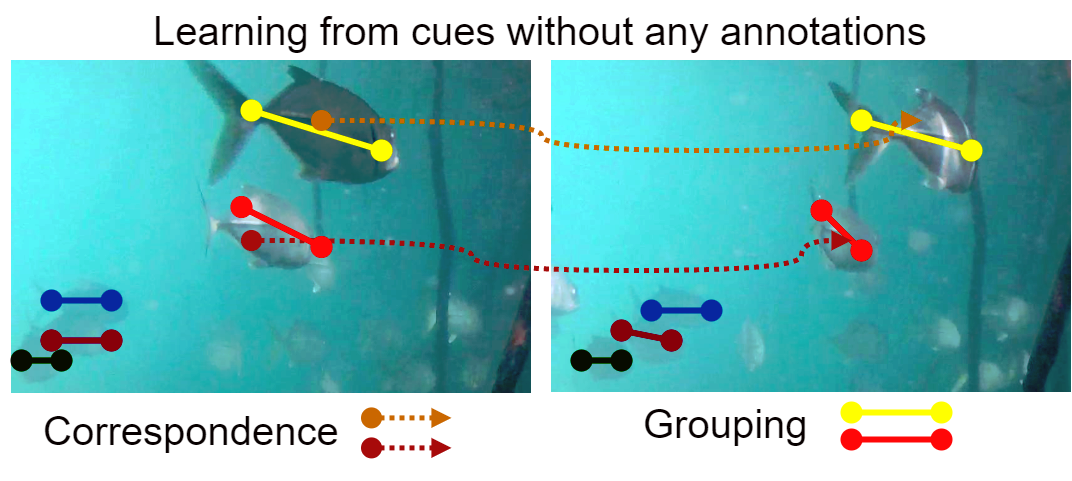
Figure 1: The natural visual artefact dynamics provide important cues about the composition of scenes, and how they change.

To that end, the primary contribution of this work is to propose an efficient self-supervised underwater fish segmentation method with good generalisability. Instead of relying on fully-supervised learning, our model can be trained in an end-to-end fashion only using unannotated input video sequences. Our proposed method is inspired by the strong performance of the self-attention mechanisms of the Transformer models. Architectures based on Transformer models, such as Vision Transformer (ViT)[5], have been shown to outperform standard Convolutional Neural Networks (CNNs) in many tasks, especially for large datasets. By combining the ViT with self-supervision, we obtain a more effective and efficient method for the task of underwater fish segmentation.

Unlike previous underwater fish segmentation methods [1, 2, 3, 4], our proposed method can achieve high-quality underwater fish segmentation without a pre-trained model or any annotations. Our work can also be seen as a specific instance of the more general segmentation methods proposed in [6, 7, 8], in the domain of underwater fish video segmentation.

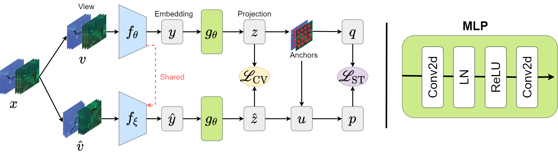
Figure 2: Our proposed framework consists of a single Transformer-based feature extractor that processes video sequences. Given a batch of unlabeled video sequences $x$, two batches of different views $v$ and $\hat{v}$ are produced and are then encoded into embeddings $y$ and $\hat{y}$ through the main branch $f_{\theta}$ and the second regularising branch $f_{\xi}$, respectively. The embeddings are fed to a multilayer perceptron (MLP) $g_{\theta}$ to produce the projections $z$ and $\hat{z}$ to compute the cross-view consistency loss $\mathcal{L}_{\text{CV}}$. The self-training loss $\mathcal{L}_{\text{ST}}$ learns space-time embeddings between the anchors $q$ and pseudo labels $p$ (arg max of $u$, affinities of $\hat{z}$ w. r. t. anchors.). The two branches are identical in architecture with shared weights. The encoders $f$ are CoaT Transformer [9] backbones.

The rest of the paper is organized as follows. Sec. II covers related works and provides background information on the novel aspects of our work. Our model’s framework is described in detail in Sec. III. Sec. IV presents our method for training and evaluating our self-supervised learning model. The experimental setup and results are presented in Sec. V, while detailed discussions of our results are presented in Sec. VI. Finally, Sec. VII concludes our paper.

II Related Work

Video object segmentation (VOS) [10, 11] without supervision has been an active area of research in recent years. Several researchers [12, 13] have exploited spatiotemporal information in videos to learn dense feature representations. In this section, we briefly review the research domains most relevant to our work.

Supervised And Unsupervised Learning. The process of learning can be either supervised or unsupervised. In the case of supervised learning [14, 15, 16, 17, 18], we have a dataset, in which each datum has a corresponding label. Therefore, the learning algorithm will be trained in such a way that it assigns the right label to the data and does not deviate from the specified label. In unsupervised learning [19, 20] on the other hand, the dataset does not include corresponding labels. Unsupervised learning tries to find the intrinsic structure in the data. For instance, previous methods [12, 13] have exploited the spatiotemporal ordering of video frames to extract supervisory signals.

In this work, we focus on unsupervised learning. Our proposed method is a self-supervised video object segmentation model trained on videos without any annotations. Therefore, there are no supervising signals (labels) available for the learning process. Hence, there is no explicit correspondence between a video and a label.

Representation learning is a class of machine learning approaches that model knowledge or representations about data (i.e. decompose training samples into feature representations) [21, 22]. Representations can be used to learn rules for classification or to represent objects that can be used for a variety of tasks such as visual object recognition, semantic understanding, and other tasks. Learning spatiotemporal representations from videos has been extensively researched [23, 24, 25, 26, 27]. However, these studies mainly learn global feature representations, not dense representations. Pinheiro et al. [28] proposed a view-agnostic model for dense representations of static scenes through pixel-level contrastive learning. In contrast to [28], which is limited to image sets of static scenes, our model learns dense representations of dynamic scenes from videos.

Contrastive Learning is a popular form of self-supervised learning [29]. It assumes visual features are invariant under a certain set of data that has two or more views and learns the representations to distinguish each view from the others. Contrastive learning approaches have also been applied to many visual classification problems in which one learns the representations invariant to scale and rotation [30, 31, 32]. Contrastive learning may also be thought of as a classification technique that classifies data by maximising feature resemblances between an image and its augmented instance, while minimising the resemblance between negative samples. For example, SimCLR [33] learns generic representations of images from an unlabeled dataset. Momentum Contrast (MoCo) [34] also exploits the negative samples on high-dimensional continuous inputs, such as images, to build a large and consistent dictionary for learning visual representations by keeping a memory bank of negative samples.

In contrast to manually augmenting the still images as in the existing contrastive methods [33, 34], we utilize the natural visual artefact changes in a natural scene directly from video data, i. e. temporally adjacent frames in videos.

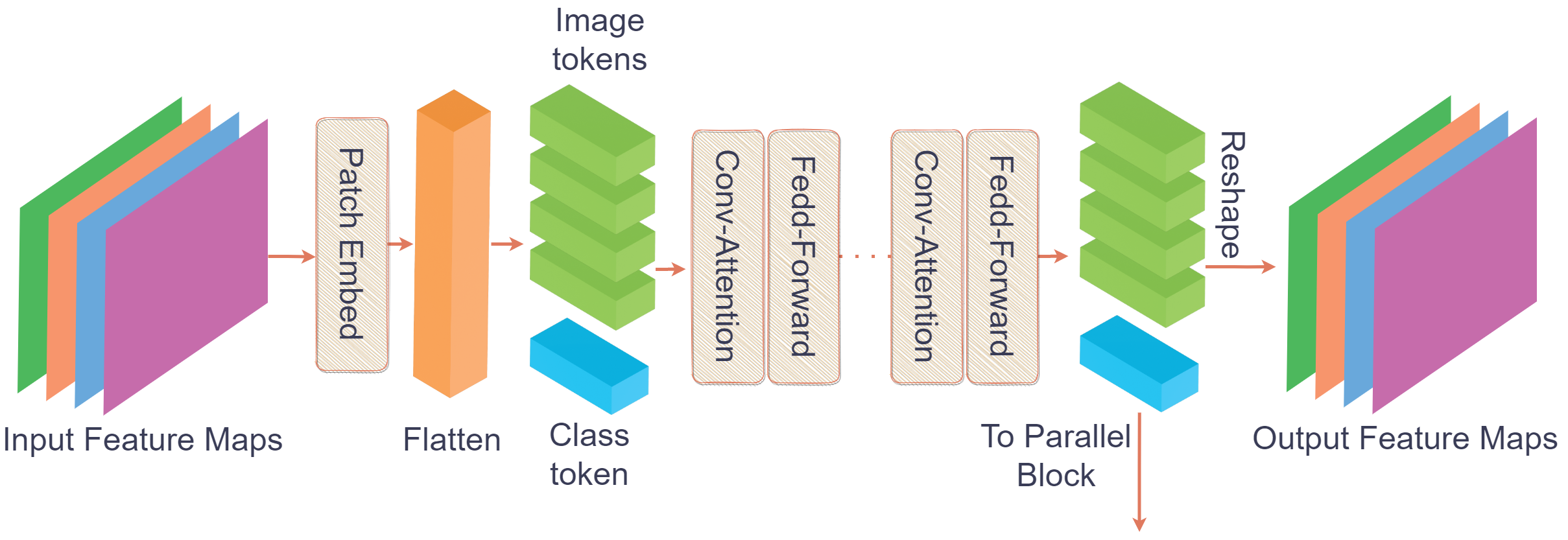
Figure 3: Schematic graph of the serial block in CoaT Transformer [9]. Input feature maps are first down-sampled by a patch embedding layer and then flatten the reduced feature maps into a sequence of image tokens. Multiple Conv-Attention and Feed-Forward layers process the tokenized features, along with a class token (a vector to achieve image classification).

Correspondence Learning aims at training a deep network by automatically predicting correspondences between image pairs [35, 36, 37]. In this way, the network can be trained with a limited number of image pairs, which eliminates the need for annotations. For instance, Fig. 1 provides an example of a spatiotemporally correlated image pair in underwater videos). When the input is a video stream, this approach is particularly useful and has recently been shown to yield interesting results [38]. Jabri et al. [6] used the contrastive random walk to learn a representation for visual correspondence from raw video. Araslanov et al. [7] took a step further by learning dense representations in a fully convolutional manner.

In contrast to [6] that uses only intra-video self-supervision, our work is similar to [8] by using both inter- and intra-video level consistency to learn more discriminatory feature embeddings.

Vision Transformers (ViT). Transformers in machine learning are composed of multiple self-attention layers. They are primarily used in natural language processing and often achieve impressive results [39]. For many computer vision applications, CNNs have long been the gold standard [40, 4, 41], yet the convolution operator makes modelling long-range interactions difficult. For this reason and due to their success in NLP, Dosovitskiy et al. [5] introduced Vision Transformer (ViT) by applying self-attention mechanisms to image patches to generate features for image classification. This approach obtained state-of-the-art results on ImageNet.

In our work, we explore attention over all possible patches in an image and the entire image at once. We apply transformer-like architectures on patches and entire images. For patches, we use $16\times 16$ grids, so that the resulting transformations can be used to generate an entire image. However, larger or smaller grids can also be used.

III Framework

An overview of our model and its training procedure is presented in Fig. 2. Given a batch of unlabeled video sequences, two batches of different views are produced and are then encoded into embeddings through the main branch and the second regularising branch. The two branches are identical in architecture with shared weights. The encoders are CoaT Transformer [9] backbones. The embeddings are fed to a multilayer perceptron (MLP) to produce the projections to compute a cross-view consistency loss, while a self-training loss helps learn space-time embeddings between introduced anchors and pseudo labels, which are explained in details below.

III-A CoaT Transformer

Our feature encoder backbone is Co-scale conv-attentional image Transformers (CoaT) [9]. CoaT is composed of two submodules: (1) a conv-attentional image transformer (CAIT) module and (2) a co-scale feature attention network (CFAN) module. The CAIT module uses a spatial transformer network and convolutional operations to produce a co-scale feature pyramid from a single input image, and to realize relative position embeddings with convolutions in the factorized attention mechanism. The CFAN network operates on top of CAIT-produced feature pyramid representations and dynamically selects informative image parts to make decisions on what to encode and what to ignore for scene understanding, allowing us to model spatial and semantic relationships at multiple scales.

CFAN is composed of two sub-modules, a serial and a parallel block, which introduce fine-to-coarse, coarse-to-fine, and cross-scale information into image transformers. The serial block (shown in Fig. 3) models image representations at a downsized resolution, while a parallel block realizes a co-scale mechanism. Given an input image $I\in\mathbb{R}^{H\times W\times C}$, each serial block down-samples the image features into lower resolution, resulting in a sequence of four resolutions:

$$F_{1}\in\mathbb{R}^{\frac{H}{4}\times\frac{W}{4}\times C_{1}},$$

$$F_{2}\in\mathbb{R}^{\frac{H}{8}\times\frac{W}{8}\times C_{2}},$$

$$F_{3}\in\mathbb{R}^{\frac{H}{16}\times\frac{W}{16}\times C_{3}},$$

$$F_{4}\in\mathbb{R}^{\frac{H}{32}\times\frac{W}{32}\times C_{4}}.$$

Since the CFAN module produces multi-scale feature attention maps from a single image, it is a more computationally efficient and scalable method than the existing multi-resolution encoder-decoder frameworks. In addition, since CFAN takes input in the form of feature pyramid representation and produces a pyramid of feature attention maps, it is more flexible than existing multi-resolution architectures that operate on fixed-sized feature pyramids.

We, therefore, use CoaT as a feature encoder in the two branches of our model, main and regularising. The main and regularising branches process two copies of the input frame batch, each of which includes the identical collection of video sequences. We feed the augmented version of each frame to the regularising branch, while the main branch receives the original video frames (as shown in Fig. 2). For augmentation, we extract random cropping and flipping, as described in Sec. IV-B. The regularising branch’s purpose is to avoid the degenerate solutions that make the network encode positional cues into a degenerate feature representation, as previously reported in[6].

III-B Multilayer Perceptron (MLP)

We pass the output from the feature encoder through a multilayer perceptron (MLP) to produce feature embeddings and to reduce the feature dimensionality from $512$ to $128$. The multilayer perceptron (MLP) code implementation in PyTorch-like style is shown in algorithm 1. The MLP consists of two standard Conv2d layers. The first layer is followed by Layer Normalisation [42] and ReLU.

⬇

1import torch.nn as nn

2

3class MLP(nn.Sequential):

4

5 def __init__(self, n_in, n_out):

6 super().__init__()

7

8 self.add_module("conv1", nn.Conv2d(n_in, n_in, 1, 1))

9 self.add_module("ln1", nn.LayerNorm(n_in))

10 self.add_module("relu", nn.ReLU(True))

11 self.add_module("conv2", nn.Conv2d(n_in, n_out, 1, 1))

Algorithm 1 Multilayer Perceptron (MLP), PyTorch-like

III-C Anchor Sampling

To improve training efficiency and computational footprint [6], we obtain $(n^{2})$ $z$-dimensional feature embeddings by defining a spatially invariant grid of size $n\!\times\!n$ on the feature tensor from the main branch $z$, and select one sample per grid cell (i. e. anchors $k$). This will make the anchors spatially distinct and cover the full feature embeddings. We then share these anchors with the regularising branch. Rather than computing pairwise distances between every feature vector in the batch, we compute the cosine similarities between the embeddings of the anchors $k$ and the current features $z$ by:

$$q_{i,j}=\tfrac{\exp(z_{i}\cdot k_{j}\mathbin{/}\tau)}{\sum\nolimits_{l}\exp(z_{i}\cdot k_{l}\mathbin{/}\tau)}$$ (1)

where $\tau\in\mathbb{R}^{+}$ is a scalar temperature hyperparameter, $z$ and $k$ are features from the main branch and the anchors, respectively, $l$ indexes batch samples and $i,j$ index the vector dimension.

For the regularising branch features, we select only the predominant anchors [7] to compute the cosine similarities as follows:

$$p_{i}=\operatorname*{arg\,max}_{j\in\mathcal{N}(i)}{\tfrac{\exp(\hat{z}_{i}\cdot k_{j}\mathbin{/}\tau)}{\sum\nolimits_{l}\exp(\hat{z}_{i}\cdot k_{l}\mathbin{/}\tau)}}\ ,$$ (2)

where $\mathcal{N}(i)$ is the index set of the anchors that stem from the same video clip as the feature vector with index $i$, and $\hat{z}$ and $k$ are features from the regularising branches and the anchors, respectively.

Note that, in Eq. 1 we extract features from multiple videos in the training batch, however, in Eq. 2 we extract features from the same video sequence only. This will help our framework to simultaneously learn intra-video (within a single video clip), and inter-video (between video clips) feature embeddings to preserve the fine-grained correspondence associations as well as instance-level feature discrimination [43].

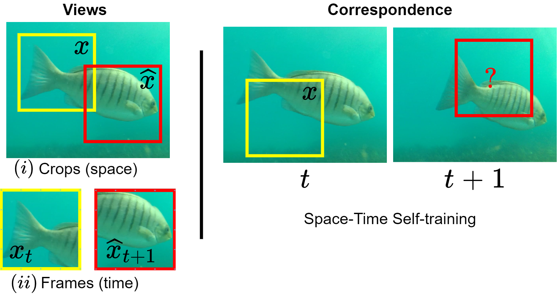
Figure 4: Representation Learning as similarity across views by discriminating features (i) spatially within individual frames and (ii) temporally, to represent each frame in a video sequence in terms of the same feature set.

III-D Loss Function

The goal of training our framework is to learn representation as similarity across views (see Fig. 4) by computing pairwise affinities between features from the model’s two branches and minimising the distance of the features extracted from the other temporally close frames to the anchors. Therefore, the overall loss of the learning algorithm is given by the following equations:

Cross-view consistency

We build the input to the regularising branch by augmenting the original video frames to generate a random similarity transformation. The corresponding change in the features output, i. e. segmentation, should be the same regardless of randomly flipping or scaling the input frame. By using the cross-view consistency loss [7] in Eq. 3 we explicitly facilitate this property.

$$\mathcal{L}_{CV}=-\sum\nolimits_{i\in\mathcal{R}}\log{\tfrac{\exp(z_{i}\cdot\hat{z}_{i}\mathbin{/}\tau)}{\sum\nolimits_{l\neq i}\exp(z_{i}\cdot\hat{z}_{l}\mathbin{/}\tau)}},$$ (3)

where $\mathcal{R}$ is the index set of the features extracted from the reference frames; $\tau\in\mathbb{R}^{+}$ is a scalar temperature hyperparameter; and $z$ and $\hat{z}$ are features from the main and the regularising branches, respectively.

Since $z$ and $\hat{z}$ are spatially coordinated, this association distinguishes the cosine similarity between the corresponding features w. r. t. non-corresponding pairs.

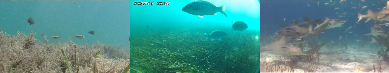
Figure 5: Sample image from each of the three utilised datasets. From left: DeepFish [44], Seagrass [45] , and YouTube-VOS [46]

Space-time self-training

After generating pseudo labels from the predominant anchor index for each feature from the regularising branch, we use space-time self-training loss [7], shown in Eq. 4, to minimise the distance between the features extracted from the original view $q$ defined by Eq. 1, and pseudo labels $p$, based on Eq. 2.

$$\mathcal{L}_{ST}=-\sum\nolimits_{i\not\in\mathcal{R}}\log\mathcal{T}(q_{i},{p_{i}})\ ,$$ (4)

where $\mathcal{R}$ is the index set of the features extracted from the reference frames, while $\mathcal{T}(\cdot)$ is random similarity transform to spatially aligns $q$ and $p$ after random cropping and flipping.

Since the anchors are a subset of features sampled spatially and temporarily from the video frames within the same view, this loss minimises the feature distance to the anchors and stimulates an increased cosine similarity of the features to the anchors and a decreased cosine similarity between the anchors themselves.

The final training objective is to minimise the combination of the above loss functions:

$$\mathcal{L}=\mathcal{L}_{CV}+\lambda\mathcal{L}_{ST},$$ (5)

where $\lambda$ is a hyperparameter that weights its contribution to the total loss.

III-E Label Propagation

We use label propagation to predict semantic labels for all video clip frames from the initial ground-truth label only. Label propagation is the task of classifying each individual pixel in the frames of a video given only ground truth for the first frame. Following previous works [6, 7, 8], we employ the representation as a similarity function for k-Nearest Neighbour (KNN) prediction.

Algorithm 2 illustrates the label propagation we use in our work. We employ context embeddings and masks acquired from previous frames to forecast the mask $m_{t}$ for the current time-step $t$. We use the output from the CoaT Transformer [9] to obtain the embedding for frame $t$. Then, we compute the cosine similarity of embedding $e_{t}$ w. r. t. all embeddings in context $\mathcal{E}$, commonly used in correlation layers of optical flow networks [47]. Next, we compute local attention in a single operation by kNN-Softmax. Finally, we update the oldest entries by replacing them with $m_{t}$ and $e_{t}$ to the mask $\mathcal{M}$ and embedding contexts $\mathcal{E}$. For the remaining frames in the video clip, we repeat the same process. Bilinear interpolation is used to bring the final object masks back to their original resolution.

Input: Embeddings $\mathcal{E}$ and mask $\mathcal{M}$ from the first frame.

Output: Mask $m_{t}$ prediction for timestep $t$.

1 for  $t$ and frame in (frames) do

2       Computing embeddings $e_{t}$ at timestep $t$;

3       Computing local spatial correlation between $\mathcal{E}$ and $e_{t}$;

4       Computing softmax between K-Nearest Neighbors;

5       Mask $m_{t}$ prediction for timestep $t$;

6       updating $\mathcal{E}$ and $\mathcal{M}$;

7      

Algorithm 2 Label Propagation

IV Method

We present the method of training and evaluating our self-supervised learning model for underwater video segmentation, using a Transformer-based feature encoder as the backbone and three datasets of real underwater videos. The model was trained on one dataset and evaluated using the other two datasets. We show that our model significantly improves over the non-transformer baseline of previous work. Finally, we show that our model is generic, and performs on video with different color distributions and scenes.

IV-A Datasets

We performed experiments using three publicly available datasets, i.e. DeepFish [44], Seagrass [45] , and YouTube-VOS [46]. Fig. 5 demonstrates a sample image from each dataset.

DeepFish [44] consists of a large number of videos collected for 20 different habitats in remote coastal marine environments of tropical Australia. The video clips were captured in full HD resolution ($1920\times 1080$ pixels) using a digital camera. In total, the number of video frames taken is about $40k$

Seagrass [45] is comprised of annotated footage of Girella tricuspidata in two estuary systems in south-east Queensland, Australia. The raw data was obtained using submerged action cameras (HD $1080p$). The dataset includes $9429$ annotations and $4280$ video frames. Each annotation includes segmentation masks that outline the species as a polygon.

YouTube-VOS [46] is a video object segmentation dataset that contains $4453$ YouTube video clips and 94 object categories. The videos have pixel-level ground truth annotations for every $5th$ frame ($6fps$). For a fair comparison, we extracted only the videos that contained fish, which include $130$ videos and $4349$ video frames in total.

We independently train our feature extractor on the DeepFish [44] dataset and evaluate it on Seagrass [45] and YouTube-VOS [46].

IV-B Data Augmentation

In addition to natural variances in the video sequences, we use similarity transformations to augment the training data (random cropping and flipping only), see Fig. 4. The reason for using these extra augmentations is to augment the same input video to feed to the second regularising branch to produce pseudo labels, see Sec. III-A.

We also experimented with several spatial and pixel-level augmentations, e. g. sheering, rotations, RGB-Shift, and colour jittering. However, we did not observe a notable change in accuracy. These augmentation methods are computationally expensive, because both rotation and sheering require image padding, which needs to be removed afterwards. Therefore, the video sequences were augmented with random flips and cropping only.

IV-C Model training

We use a Transformer-based feature encoder as the backbone network for our feature extractor (see Sec. III-A). As a baseline, we adopt the ResNet-18 feature encoder [48]) as used in [6, 7, 8]. Similar to [6, 7, 8], we also remove the strides in the res3 and res4 blocks from the ResNet-18 architecture. Both our proposed Transformer-based and baseline models’ weights were randomly initialised.

Our models were trained with an input resolution of $256\times 256$ pixels. We scale the lowest side of the video frames to $256$ and then extract random crops of size $256\times 256$. We sample two video sets, $B=2$ (of size $T=5$ frames), therefore, $B\times T=2\times 5=10$ frames are used per forward pass.

We found that for this problem set, a learning rate of $1\times 10^{-3}$ works the best. It took around 300 epochs for all models to train on this problem. Our networks were trained on a Linux host with a single NVidia GeForce RTX 2080 Ti GPU with $11$ GB of memory, using Pytorch framework [49]. We used Adam optimiser [50] with $\beta_{1}=0.5$, $\beta_{2}=0.999$, and $\epsilon=1.0\times 10^{-08}$. We applied the same hyperparameter configuration for all of the models. However, the optimum model configuration will depend on the application, hence, these results are not intended to represent a complete search of model configurations. Our training loop is shown in algorithm 3.

Input: Unlabeled video sequences.

Output: Trained weights for the backbone network.

1 for each mini-batch do

2       Extract deep features of the video frames;

3       Regularising branch produces pseudo labels;

4      

5      for each video in the mini-batch do

6             // Transformer-based encoder

7             Extract feature embeddings (anchors) $k$;

8             Compute affinity to anchors ${q}$ (Eq. 1);

9             Compute pseudo labels ${q}$ (Eq. 2);

10            

11            // Loss Computation

12             Compute Cross-view consistency $\mathcal{L}_{\text{CV}}$ (Eq. 3);

13             Compute Space-time self-training $\mathcal{L}_{\text{ST}}$ (Eq. 4);

14             Compute total loss $\mathcal{L}$ (Eq. 5);

15            

16      Back-propagate all the losses in this mini-batch;

17      

Algorithm 3 Main Training Loop

IV-D Inference

At the inference time, we compute dense correspondences for video propagation using the learned encoder’s representation. The encoder’s representation is the trained weights for the backbone network (see Sec. III-A and Algorithm 3). We predict the whole video frames segmentation masks using Label Propagation (Sec. III-E). Given the initial ground-truth segmentation mask of the first frame, we label propagate the rest of the frames in the video without the need for the rest of ground-truth annotations. The labels are propagated in the feature space. The labels in the first frame are one-hot vectors, whereas the labels propagated are Softmax distributions.

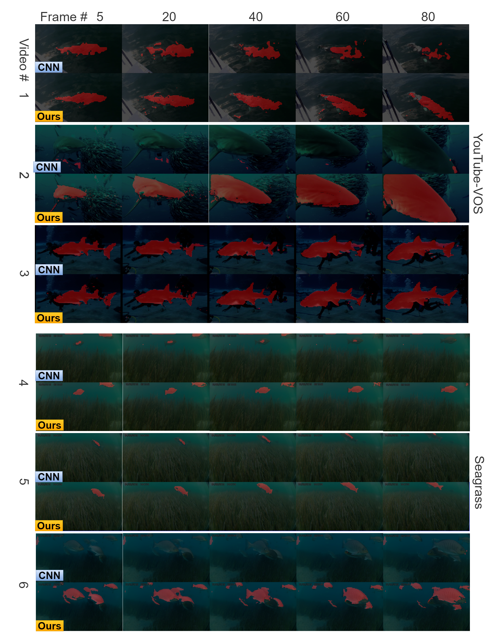
Figure 6: Qualitative examples of our model applied on the YouTube-VOS [46] (the top 3 panels), and Seagrass [45] (the bottom 3 panels) datasets. The representation learned by our method effectively distinguishes between objects and background ambiguity and is robust to occlusions.

V Experiments

We report experimental results for our model’s trained representation on the DeepFish dataset and evaluate on Seagrass and YouTube-VOS datasets without fine-tuning. We provide quantitative and qualitative results that demonstrate our model’s generalization capabilities to a range of different underwater habitats.

V-A Performance Comparison

To evaluate on Seagrass [45] and YouTube-VOS [46], we independently train our feature extractor on DeepFish [44], which compared to the other datasets contains more video sequences, as discussed in Sec. IV-A. For a fair comparison, the frames are processed at a resolution of 480p.

Table I reports the result of a quantitative analysis, where the best results for each metric are in bold. We measure the segmentation accuracy in terms of two types of metrics: 1) The Jaccard’s index ($\mathcal{J}$), measures the region similarity as Intersection-over-Union (IoU) between the object and the mask. 2) Alignment of boundary metric ($\mathcal{F}$), measures the region contour. Specifically, we report the mean ($\mathcal{J}_{m}$, $\mathcal{F}_{m}$), the recall ($\mathcal{J}_{r}$, $\mathcal{F}_{r}$), and the mean average ${\mathcal{J}\&\mathcal{F}}_{m}$, with an IoU threshold of $0.5$.

Compared to the baseline ResNet-18 CNN [7], our approach reaches a higher ${\mathcal{J}\&\mathcal{F}}_{m}$ score by $4.5\%$ and $3.1\%$ on Seagrass and YouTube-VOS, respectively. This is mainly caused by the use of self-attention mechanisms that can extract high-level spatial features for the segmentation of long-range video sequences. Moreover, the self-attention layers can be used to model the dependency among multiple temporal steps, which is helpful for the segmentation of objects having large motions.

TABLE I: Performance Comparison on Seagrass [45] and YouTube-VOS [46] datasets.

Method	$\mathcal{J}{\&}\mathcal{F}_{\textrm{m}}$	$\mathcal{J}_{\textrm{m}}$	$\mathcal{J}_{\textrm{r}}$	$\mathcal{F}_{\textrm{m}}$	$\mathcal{F}_{\textrm{r}}$
Seagrass [45]
1-7
CNN [7]	45.5	40.2	41.0	50.7	54.7
Transformer (ours)	50.0	41.5	43.3	58.1	65.4
YouTube-VOS [46]
1-7
CNN [7]	60.2	60.9	72.7	59.5	70.0
Transformer (ours)	63.3	63.9	74.0	62.7	69.6

V-B Qualitative Results

Fig. 6 shows the qualitative results of our model using the YouTube-VOS [46] (top-3 panels) and the Seagrass [45] (bottom-3 panels). It is evident that our proposed method produces significantly higher quality results compared to the CNN-based encoder [7]. An apparent advantage of our model shown in the bottom panel is its ability to segment multiple and overlapping fish, in the scene, where its CNN counterpart fails. Fig. 6 also shows that our model is stable and can effectively locate fish despite complex scenes. The CNN-based method, on the other hand, has the problem of failing to predict the segmentation in some situations when there is vagueness between the foreground object and the background, or when there are complex transformations in the videos. Whereas our method shows a strong ability to differentiate pixels with similar intensities. Furthermore, these quantitative results show that our proposed method can work on datasets with very small objects (see Videos 4 and 5 in Fig. 6).

V-C Ablation Study

To further investigate the effect of our proposed transformer-based video segmentation framework, we performed an ablation study. In this study, we compared the baseline CNN model (no transformers) [7] and our Transformer-based feature encoder, with different types of transformers. For these comparisons, we used different configurations of video features, Transformers, and MPL layers, to find out which combination results in the best performance. We report only results with best configurations.

Table II reports the segmentation accuracy for four different models in terms of ${\mathcal{J}\&\mathcal{F}}_{m}$ metric, in addition to the base-line CNN [7] and our proposed models discussed in Sec. V. In this Table, the second line is the Fast Fourier Convolution model in [51]. The third line refers to the Transformer for Semantic Segmentation introduced in [52], while the fourth line reports the MetaFormer-based architecture called PoolFormer [53]. The fifth line is for Cross-Covariance Image Transformer (XCiT) [54].We also report the FCN for semantic segmentation [55] as a fully-supervised learning method.

Based on the evaluation in Table II, our Transformer-based model significantly outperforms the baseline and other meta-architecture methods in the context of both datasets.

TABLE II: Ablation study for other models on Seagrass [45] and YouTube-VOS [46] datasets.

	$\mathcal{J}{\&}\mathcal{F}_{\textrm{mean}}$
Method	Seagrass [45]	YouTube-VOS [46]
Baseline [7]	45.5	60.2
FFC [51]	46.2	60.6
Segmenter [52]	41.5	52.7
PoolFormer [53]	42.8	54.9
XCiT [54]	43.7	56.8
Transformer (ours)	50.0	63.3
1-4 Fully-supervised [55]	64.7	79.3

VI Discussion

The main goal of this study was to improve underwater fish segmentation performance without using any human labels. We proposed an end-to-end underwater fish segmentation method with self-supervised learning, by combining the Transformer self-attention mechanisms with self-supervised learning. Our method improves fish segmentation performance for different fish shapes, in different underwater scenarios, on different videos, or for different fish species, without relying on a large set of segmentation-level annotations.

Unlike the baseline model with CNN-based feature encoders, our proposed transformer-based encoder is robust to occlusion and can recognize most fish classes, regardless of the distance from the camera. We demonstrated that when combined with self-supervised learning, our transformer-based encoder model outperforms several other CNN- and transformer-based architectures in terms of pixel-level underwater fish segmentation. Our proposed method uses only RGB frames as input and extracts useful information from large training datasets. During inference, only one frame is required to produce results for a given input video. In future works, we intend to conduct additional experiments using a larger dataset as a source of self-supervision.

Our framework is computationally efficient because it learns dense representations, not global feature representations at the video level. Due to this, our model can be trained on a single 11GB GPU, which is a significant improvement compared to the prior art.

Another advantage of our framework is that it does not require a pre-trained model. We trained our initial transformer-based model from scratch using self-supervision on the DeepFish dataset, and tested it on the Seagrass and YouTube-VOS datasets without any new pre-trained model, showcasing the strong generalisability of our model and framework.

Despite the above-mentioned advantages, the main limitation of our study is that it only focuses on the case of underwater fish segmentation. Further work and future research are required to investigate segmentation of for other underwater object. Another limitation of our study is the scarcity of its training data. We rely on the existing training data and a relatively small number of test videos to evaluate our proposed method. However, we hope that this work will inspire further research that may use larger datasets.

In future work, we will try to expand the scope of our proposed model by adding more datasets and tasks, such as underwater object tracking and counting, since the self-supervised learning model can be viewed as a generic tool for underwater video processing, which is critical in underwater fish habitat monitoring [56] and the internet of underwater things [57].

VII Conclusion

We proposed a novel method for underwater fish segmentation using the combination of self-supervised learning and a transformer encoder that is trained without manual annotations. Our method outperforms previous models in underwater video segmentation in the wild, is more efficient, and does not require pre-trained models. It can generalize well even without using additional training data. It can be used to automatically analyse underwater video streams and detect rare and endangered species. It can also assist with species distribution, stock management, and fishing enforcement. In the future, our method could provide a foundation for self-supervised learning to facilitate underwater fish habitat monitoring in marine and aquaculture farm settings.We also intend to conduct additional experiments on larger underwater fish datasets and expand the capabilities of our proposed segmentation model.

References

- [1] R. Garcia, R. Prados, J. Quintana, A. Tempelaar, N. Gracias, S. Rosen, H. Vågstøl, and K. Løvall, “Automatic segmentation of fish using deep learning with application to fish size measurement,” ICES Journal of Marine Science, 2020.
- [2] C. C. Chang, Y. P. Wang, and S. C. Cheng, “Fish segmentation in sonar images by mask r-cnn on feature maps of conditional random fields†,” Sensors, 2021.
- [3] N. F. F. Alshdaifat, A. Z. Talib, and M. A. Osman, “Improved deep learning framework for fish segmentation in underwater videos,” Ecological Informatics, vol. 59, p. 101121, 2020.
- [4] I. H. Laradji, A. Saleh, P. Rodriguez, D. Nowrouzezahrai, M. R. Azghadi, and D. Vazquez, “Weakly supervised underwater fish segmentation using affinity LCFCN.” Scientific reports, vol. 11, no. 1, p. 17379, 12 2021. [Online]. Available: https://www.nature.com/articles/s41598-021-96610-2http://www.ncbi.nlm.nih.gov/pubmed/34462458http://www.pubmedcentral.nih.gov/articlerender.fcgi?artid=PMC8405733
- [5] A. Dosovitskiy, L. Beyer, A. Kolesnikov, D. Weissenborn, X. Zhai, T. Unterthiner, M. Dehghani, M. Minderer, G. Heigold, S. Gelly, J. Uszkoreit, and N. Houlsby, “An Image is Worth 16x16 Words: Transformers for Image Recognition at Scale,” IEEE, 10 2020. [Online]. Available: http://arxiv.org/abs/2010.11929
- [6] A. A. Jabri, A. Owens, and A. A. Efros, “Space-time correspondence as a contrastive random walk,” in Advances in Neural Information Processing Systems, 2020.
- [7] N. Araslanov, S. Schaub-Meyer, and S. Roth, “Dense Unsupervised Learning for Video Segmentation,” 11 2021. [Online]. Available: https://arxiv.org/abs/2111.06265v1
- [8] N. Wang, W. Zhou, and H. Li, “Contrastive Transformation for Self-supervised Correspondence Learning,” 12 2020. [Online]. Available: https://arxiv.org/abs/2012.05057v1
- [9] W. Xu, Y. Xu, T. Chang, and Z. Tu, “Co-Scale Conv-Attentional Image Transformers,” in 2021 IEEE/CVF International Conference on Computer Vision (ICCV). IEEE, 10 2021, pp. 9961–9970. [Online]. Available: https://ieeexplore.ieee.org/document/9710209/
- [10] R. Yao, G. Lin, S. Xia, J. Zhao, and Y. Zhou, “Video Object Segmentation and Tracking,” 2020.
- [11] K. Xu, L. Wen, G. Li, and Q. Huang, “Self-Supervised Deep TripleNet for Video Object Segmentation,” IEEE Transactions on Multimedia, 2021.
- [12] B. Fernando, H. Bilen, E. Gavves, and S. Gould, “Self-supervised video representation learning with odd-one-out networks,” in Proceedings - 30th IEEE Conference on Computer Vision and Pattern Recognition, CVPR 2017, 2017.
- [13] D. Wei, J. Lim, A. Zisserman, and W. T. Freeman, “Learning and Using the Arrow of Time,” in Proceedings of the IEEE Computer Society Conference on Computer Vision and Pattern Recognition, 2018.
- [14] T. Jiang, J. L. Gradus, and A. J. Rosellini, “Supervised Machine Learning: A Brief Primer,” Behavior Therapy, 2020.
- [15] X. Wang, X. Lin, and X. Dang, “Supervised learning in spiking neural networks: A review of algorithms and evaluations,” Neural Networks, 2020.
- [16] A. Saleh, I. H. Laradji, D. A. Konovalov, M. Bradley, D. Vazquez, and M. Sheaves, “A realistic fish-habitat dataset to evaluate algorithms for underwater visual analysis,” Scientific Reports, vol. 10, no. 1, p. 14671, 12 2020. [Online]. Available: http://www.ncbi.nlm.nih.gov/pubmed/32887922http://www.pubmedcentral.nih.gov/articlerender.fcgi?artid=PMC7473859https://www.nature.com/articles/s41598-020-71639-x
- [17] D. A. Konovalov, A. Saleh, D. B. Efremova, J. A. Domingos, and D. R. Jerry, “Automatic Weight Estimation of Harvested Fish from Images,” in 2019 Digital Image Computing: Techniques and Applications, DICTA 2019. Institute of Electrical and Electronics Engineers Inc., 12 2019.
- [18] D. A. Konovalov, A. Saleh, J. A. Domingos, R. D. White, and D. R. Jerry, “Estimating Mass of Harvested Asian Seabass Lates calcarifer from Images,” World Journal of Engineering and Technology, vol. 6, no. 03, p. 15, 2018.
- [19] I. Croitoru, S. V. Bogolin, and M. Leordeanu, “Unsupervised Learning of Foreground Object Segmentation,” International Journal of Computer Vision, 2019.
- [20] M. Längkvist, L. Karlsson, and A. Loutfi, “A review of unsupervised feature learning and deep learning for time-series modeling,” Pattern Recognition Letters, 2014.
- [21] Y. Bengio, A. Courville, and P. Vincent, “Representation learning: A review and new perspectives,” IEEE Transactions on Pattern Analysis and Machine Intelligence, 2013.
- [22] A. Kolesnikov, X. Zhai, and L. Beyer, “Revisiting self-supervised visual representation learning,” in Proceedings of the IEEE Computer Society Conference on Computer Vision and Pattern Recognition, 2019.
- [23] Y. Bai, H. Fan, I. Misra, G. Venkatesh, Y. Lu, Y. Zhou, Q. Yu, V. Chandra, and A. Yuille, “Can Temporal Information Help with Contrastive Self-Supervised Learning?” 11 2020. [Online]. Available: https://arxiv.org/abs/2011.13046v1http://arxiv.org/abs/2011.13046
- [24] P. Sermanet, C. Lynch, Y. Chebotar, J. Hsu, E. Jang, S. Schaal, S. Levine, and G. Brain, “Time-Contrastive Networks: Self-Supervised Learning from Video,” in Proceedings - IEEE International Conference on Robotics and Automation, 2018.
- [25] J. Shao, X. Wen, B. Zhao, and X. Xue, “Temporal Context Aggregation for Video Retrieval with Contrastive Learning,” in 2021 IEEE Winter Conference on Applications of Computer Vision (WACV). IEEE, 1 2021, pp. 3267–3277. [Online]. Available: https://ieeexplore.ieee.org/document/9423060/
- [26] F. Han, J. Yao, H. Zhu, and C. Wang, “Marine Organism Detection and Classification from Underwater Vision Based on the Deep CNN Method,” Mathematical Problems in Engineering, 2020.
- [27] J. Wang, J. Jiao, and Y. H. Liu, “Self-supervised Video Representation Learning by Pace Prediction,” in Lecture Notes in Computer Science (including subseries Lecture Notes in Artificial Intelligence and Lecture Notes in Bioinformatics), 2020.
- [28] P. O. Pinheiro, A. Almahairi, R. Y. Benmalek, F. Golemo, and A. Courville, “Unsupervised Learning of Dense Visual Representations,” Advances in Neural Information Processing Systems, 11 2020. [Online]. Available: http://arxiv.org/abs/2011.05499
- [29] A. Jaiswal, A. R. Babu, M. Z. Zadeh, D. Banerjee, and F. Makedon, “A Survey on Contrastive Self-Supervised Learning,” Technologies, 2020.
- [30] P. H. Le-Khac, G. Healy, and A. F. Smeaton, “Contrastive Representation Learning: A Framework and Review,” IEEE Access, 2020.
- [31] M. Ye, X. Zhang, P. C. Yuen, and S.-F. Chang, “Unsupervised Embedding Learning via Invariant and Spreading Instance Feature,” in 2019 IEEE/CVF Conference on Computer Vision and Pattern Recognition (CVPR). IEEE, 6 2019, pp. 6203–6212. [Online]. Available: https://ieeexplore.ieee.org/document/8953747/
- [32] D. Xiao, C. Qin, H. Yu, Y. Huang, and C. Liu, “Unsupervised deep representation learning for motor fault diagnosis by mutual information maximization,” Journal of Intelligent Manufacturing, vol. 32, no. 2, pp. 377–391, 2 2021. [Online]. Available: https://link.springer.com/10.1007/s10845-020-01577-y
- [33] T. Chen, S. Kornblith, K. Swersky, M. Norouzi, and G. Hinton, “Big self-supervised models are strong semi-supervised learners,” arXiv preprint arXiv:2006.10029, 2020.
- [34] K. He, H. Fan, Y. Wu, S. Xie, and R. Girshick, “Momentum Contrast for Unsupervised Visual Representation Learning,” in Proceedings of the IEEE Computer Society Conference on Computer Vision and Pattern Recognition, 2020.
- [35] T. Schmidt, R. Newcombe, and D. Fox, “Self-Supervised Visual Descriptor Learning for Dense Correspondence,” IEEE Robotics and Automation Letters, 2017.
- [36] Z. Lai and W. Xie, “Self-supervised learning for video correspondence flow,” in 30th British Machine Vision Conference 2019, BMVC 2019, 2020.
- [37] X. Li, S. Liu, S. de Mello, X. Wang, J. Kautz, and M. H. Yang, “Joint-task self-supervised learning for temporal correspondence,” in Advances in Neural Information Processing Systems, 2019.
- [38] Z. Lai, E. Lu, and W. Xie, “MAST: A memory-augmented self-supervised tracker,” in Proceedings of the IEEE Computer Society Conference on Computer Vision and Pattern Recognition, 2020.
- [39] A. Vaswani, N. Shazeer, N. Parmar, J. Uszkoreit, L. Jones, A. N. Gomez, L. Kaiser, and I. Polosukhin, “Attention is all you need,” arXiv preprint arXiv:1706.03762, 2017.
- [40] D. A. Konovalov, A. Saleh, M. Bradley, M. Sankupellay, S. Marini, and M. Sheaves, “Underwater Fish Detection with Weak Multi-Domain Supervision,” in 2019 International Joint Conference on Neural Networks (IJCNN), vol. 2019-July. IEEE, 7 2019, pp. 1–8. [Online]. Available: https://ieeexplore.ieee.org/document/8851907/
- [41] A. Saleh, I. H. Laradji, C. Lammie, D. Vazquez, C. A. Flavell, and M. R. Azghadi, “A Deep Learning Localization Method for Measuring Abdominal Muscle Dimensions in Ultrasound Images,” IEEE Journal of Biomedical and Health Informatics, vol. 25, no. 10, pp. 3865–3873, 10 2021. [Online]. Available: https://ieeexplore.ieee.org/document/9444630/
- [42] J. L. Ba, J. R. Kiros, and G. E. Hinton, “Layer Normalization,” 7 2016. [Online]. Available: https://arxiv.org/abs/1607.06450v1
- [43] N. Wang, W. Zhou, and H. Li, “Contrastive Transformation for Self-supervised Correspondence Learning,” 12 2020. [Online]. Available: https://arxiv.org/abs/2012.05057v1
- [44] A. Saleh, I. H. Laradji, D. A. Konovalov, M. Bradley, D. Vazquez, and M. Sheaves, “A realistic fish-habitat dataset to evaluate algorithms for underwater visual analysis,” Scientific Reports, vol. 10, no. 1, p. 14671, 12 2020. [Online]. Available: https://www.nature.com/articles/s41598-020-71639-x
- [45] E. M. Ditria, R. M. Connolly, E. L. Jinks, and S. Lopez-Marcano, “Annotated Video Footage for Automated Identification and Counting of Fish in Unconstrained Seagrass Habitats,” Frontiers in Marine Science, vol. 8, 3 2021. [Online]. Available: https://www.frontiersin.org/articles/10.3389/fmars.2021.629485/full
- [46] N. Xu, L. Yang, Y. Fan, J. Yang, D. Yue, Y. Liang, B. Price, S. Cohen, and T. Huang, “YouTube-VOS: Sequence-to-Sequence Video Object Segmentation,” in Lecture Notes in Computer Science (including subseries Lecture Notes in Artificial Intelligence and Lecture Notes in Bioinformatics), 2018.
- [47] D. Sun, X. Yang, M.-Y. Liu, and J. Kautz, “PWC-Net: CNNs for Optical Flow Using Pyramid, Warping, and Cost Volume,” in 2018 IEEE/CVF Conference on Computer Vision and Pattern Recognition. IEEE, 6 2018, pp. 8934–8943. [Online]. Available: https://ieeexplore.ieee.org/document/8579029/
- [48] K. He, X. Zhang, S. Ren, and J. Sun, “Deep Residual Learning for Image Recognition,” Computer Vision and Pattern Recognition (CVPR), 2015.
- [49] A. Paszke, S. Gross, F. Massa, A. Lerer, J. Bradbury, G. Chanan, T. Killeen, Z. Lin, N. Gimelshein, L. Antiga, A. Desmaison, A. Köpf, E. Yang, Z. DeVito, M. Raison, A. Tejani, S. Chilamkurthy, B. Steiner, L. Fang, J. Bai, and S. Chintala, “PyTorch: An imperative style, high-performance deep learning library,” in Advances in Neural Information Processing Systems, 2019.
- [50] D. P. Kingma and J. Ba, “Adam: A method for stochastic optimization,” arXiv preprint arXiv:1412.6980, 2014.
- [51] L. Chi, B. Jiang, and Y. Mu, “Fast Fourier Convolution,” in Advances in Neural Information Processing Systems, H. Larochelle, M. Ranzato, R. Hadsell, M. F. Balcan, and H. Lin, Eds., vol. 33. Curran Associates, Inc., 2020, pp. 4479–4488. [Online]. Available: https://proceedings.neurips.cc/paper/2020/file/2fd5d41ec6cfab47e32164d5624269b1-Paper.pdf
- [52] R. Strudel, R. Garcia, I. Laptev Inria, and C. Schmid Inria, “Segmenter: Transformer for Semantic Segmentation,” 5 2021. [Online]. Available: https://arxiv.org/abs/2105.05633v3
- [53] W. Yu, M. Luo, P. Zhou, C. Si, Y. Zhou, X. Wang, J. Feng, and S. Yan, “MetaFormer is Actually What You Need for Vision,” 11 2021. [Online]. Available: https://arxiv.org/abs/2111.11418v2
- [54] A. El-Nouby, H. Touvron, M. Caron, P. Bojanowski, M. Douze, A. Joulin, I. Laptev, N. Neverova, G. Synnaeve, J. Verbeek, and H. Jegou, “XCiT: Cross-Covariance Image Transformers,” 6 2021. [Online]. Available: https://arxiv.org/abs/2106.09681v2
- [55] E. Shelhamer, J. Long, and T. Darrell, “Fully Convolutional Networks for Semantic Segmentation,” IEEE Transactions on Pattern Analysis and Machine Intelligence, vol. 39, no. 4, pp. 640–651, 4 2017.
- [56] A. Saleh, M. Sheaves, and M. Rahimi Azghadi, “Computer vision and deep learning for fish classification in underwater habitats: A survey,” Fish and Fisheries, 4 2022. [Online]. Available: https://onlinelibrary.wiley.com/doi/10.1111/faf.12666
- [57] M. Jahanbakht, W. Xiang, L. Hanzo, and M. R. Azghadi, “Internet of Underwater Things and Big Marine Data Analytics - A Comprehensive Survey,” IEEE Communications Surveys and Tutorials, vol. 23, no. 2, pp. 904–956, 2021. [Online]. Available: https://ieeexplore.ieee.org/document/9328873/