Ring Seismology of the Ice Giants Uranus and Neptune

Abstract

We assess the prospect of using ring seismology to probe the interiors of the ice giants Uranus and Neptune. We do this by calculating normal mode spectra for different interior models of Uranus and Neptune using the stellar oscillation code GYRE. These spectra provide predictions of where in these planets’ ring systems the effects of interior oscillations might be detected. We find that f-mode resonances with azimuthal order $m=2$ or $7\leq m\leq 19$ fall among the inner rings (6, 5, 4, $\alpha$, and $\beta$) of Uranus, while f-mode resonances with $2\leq m\leq 12$ fall in the tenuous $\zeta$ ring region. In addition, f-mode resonances with $m=2$ or $6\leq m\leq 13$ may give azimuthal structure to Neptune’s tenuous Galle ring. We also find that g-mode resonances may fall in the middle to outer rings of these planets. Although an orbiter is most likely required to confirm the association between any waves in the rings and planetary normal modes, the diversity of normal mode spectra implies that identification of just one or two modes in the rings of Uranus or Neptune would eliminate a variety of interior models, and thus aid in the interpretation of Voyager observations and future spacecraft measurements.

1 Introduction

Three decades after the Voyager flybys of Uranus and Neptune, our knowledge of their internal structure and composition is still quite limited (Helled & Fortney, 2020). The ice giants Uranus and Neptune represent a distinct class of planets with radii between those of terrestrial worlds like Earth and Venus and gas giants like Jupiter and Saturn. The recent discovery that Neptune-mass exoplanets are common (Suzuki et al., 2016) motivates the exploration of the ice giants in our own solar system.

The deep interiors of the ice giants Uranus and Neptune are of special interest because their internal structure and composition are distinct from the gas giants Jupiter and Saturn. Their measured densities suggest that Uranus and Neptune have substantial amounts of carbon, nitrogen, oxygen, sulfur, and silicon, which form compounds like water, ammonia, methane, and silicate minerals (Podolak et al., 2019). At the high pressures and temperatures of planetary interiors, these “rocks” and “ices” display interesting properties. Water, for example, can enter a superionic state where the oxygen atoms become a lattice and the hydrogen nuclei are free to move, which may play a role in explaining the non-axisymmetric non-dipolar magnetic fields of Uranus and Neptune (Cavazzoni et al., 1999; Wilson et al., 2013). Although numerical calculations and laboratory experiments are providing better constraints on these exotic phases of these materials (Knudson et al., 2012; Bethkenhagen et al., 2017; Millot et al., 2018, 2019; French & Nettelmann, 2019), and methods to constrain interiors through high-precision gravity measurements are being developed (Movshovitz & Fortney, 2022), there remain many uncertainties regarding important parameters such as the mixing properties of the various compounds. In addition, both the overall breakdown and spatial distributions of hydrogen, helium, water, ammonia, methane, and silicates within the planets are poorly constrained.

While the interiors of Uranus and Neptune remain largely hidden, their ring systems are available for easier observation. Recent analyses of Saturn’s rings have demonstrated that certain ring features are likely generated by resonances with normal modes inside the planet (Hedman & Nicholson, 2013, 2014; French et al., 2016, 2019; Hedman et al., 2019; French et al., 2021; Hedman et al., 2022), confirming predictions made by Marley & Porco (1993) and providing new insights into that planet’s interior. Furthermore, Marley et al. (1988) performed preliminary calculations and found that resonances with a few Uranian normal modes could potentially fall close to some of the Uranian rings (see Table 6 in the Appendices). This paper therefore seeks to build upon that work and establish which planetary normal modes are most likely to fall close to the rings of Uranus and Neptune and thus are the most promising candidates for performing ring seismology at the ice giants.

In Section 2, we provide a brief overview of ring seismology and summarize the current state of knowledge about the ring systems. In Section 3, we describe the interior models that we use, and then we explain how we analyze the gravitational potential and calculate the resonance locations. In Section 4, we report the locations of these resonances and compare them with relevant structures in the ring systems of the two planets. In Section 5, we discuss which of the planetary normal mode resonances are most likely to be detectable in the rings, with remarks on several individual rings of interest. Complete tables of mode frequencies and associated resonance locations are provided in the Appendices.

2 Background

Before describing our methods for computing normal mode resonance locations, we first provide a brief overview of giant planet seismology in Subsection 2.1 and the relevant features in the rings of Uranus and Neptune in Subsection 2.2.

2.1 Overview of Ring Seismology

Planetary oscillations can be decomposed into a set of normal modes, each of which oscillates at a frequency that depends on the planet’s profiles of density, adiabatic sound speed, and rotation frequency. Familiar families of oscillation modes include g-modes, whose restoring force is buoyancy, and p-modes, whose restoring force is pressure. Three numbers characterize planetary normal-mode oscillations: the number of radial nodes $n$, the spherical harmonic degree $\ell$, and the azimuthal wavenumber $m$. In this paper, we adopt the convention that $m>0$ correspond to prograde modes, i.e. modes that propagate in the same direction as the planet’s rotation. While the mode amplitude spectrum is generally unknown, for the simplest assumption of energy equipartition, the strongest perturbations in the planet’s gravitational field are produced by the fundamental modes ($n=0$; f-modes), which can arise from a combination of predominantly gravity but also pressure as the restoring force (Unno et al., 1979). Saturn’s f-modes, for example, produce the most obvious features in its rings (Hedman & Nicholson, 2013, 2014; French et al., 2016, 2019, 2020; Hedman et al., 2019), as predicted by Marley & Porco (1993). For this reason, we will primarily consider the f-modes here.

Because the oscillation frequencies depend on the planet’s density profile, measurements of these frequencies can probe the planet’s internal structure. Efforts to detect oscillations with visible photometry, which were apparently successful for Jupiter (Gaulme et al., 2011), have not yet been successful for the ice giants (Rowe et al., 2017; Gaulme, 2017). Friedson (2020) found that for reasonable amplitudes, detection of pressure or temperature variations due to ice giant normal modes is not as promising as the prospect of detecting their gravitational influence on an orbiting spacecraft.

Fortunately, we can potentially also detect planetary normal modes by treating the ring material that orbits the planet as a seismograph. Any even $\ell-m$ mode is symmetric about the equator and would generate a Lindblad resonance in ring material, which excites density waves; whereas any odd $\ell-m$ mode is antisymmetric about the equator and would generate a vertical resonance, which excites bending waves. The $\ell=m$ modes are the modes that are expected to be the most easily observable at their Lindblad resonance locations because the amplitude of the gravitational perturbation in the ring plane suffers no destructive interference due to latitudinal variations in the phase of the planetary oscillation. Because Saturn’s rings are the largest in our solar system and the dataset on them was the most extensive, they were naturally the first target for ring seismology. Voyager images and radio occultation profiles of Saturn’s rings revealed spiral density waves and bending waves. Some of these waves could be explained in terms of resonances with Saturn’s moons, but other waves in the C ring were far from any known satellite resonance (Rosen et al., 1991). Meanwhile, Marley (1991) and Marley & Porco (1993), building upon ideas from Stevenson (1982), showed that certain normal modes in Saturn’s interior could cause gravitational perturbations in the C ring, and proposed potential correlations between some of the waves and specific planetary f-modes. Once the Cassini mission arrived at Saturn, new waves were detected (Baillié et al., 2011) and several features were confirmed to be generated by resonances with planetary oscillations and asymmetries (Hedman & Nicholson, 2013, 2014; French et al., 2016, 2019; Hedman et al., 2019; French et al., 2021; Hedman et al., 2022). These studies yielded the azimuthal wavenumber and the precise frequency for a set of planetary normal modes that provide evidence for a stably stratified layer within the planet (Fuller, 2014), an estimate for Saturn’s bulk rotation rate (Mankovich et al., 2019), evidence for a diffuse core (Mankovich & Fuller, 2021), and constraints on differential rotation (Dewberry et al., 2021).

2.2 The Rings and Inner Moons of Uranus and Neptune

Table 1 displays the semi-major axes and eccentricities of the thirteen innermost Uranian moons and the seven innermost Neptunian moons. Table 2 shows the semi-major axes and widths of the inner Uranian and Neptunian rings.

The Uranian ring system includes three broad rings ($\zeta$, $\nu$, and $\mu$) and ten narrow rings (6, 5, 4, $\alpha$, $\beta$, $\eta$, $\gamma$, $\delta$, $\lambda$, and $\epsilon$). The innermost Uranian moons, Cordelia and Ophelia, each with diameters of $\sim 40$ km (Karkoschka, 2001), flank the $\lambda$ and $\epsilon$ rings and play a role in shepherding the $\epsilon$ ring (French et al., 1991). The narrow rings except the $\lambda$ ring are optically thick at visible wavelengths and are expected to be dominated by centimeter- to meter-sized particles (Nicholson et al., 2018). Several small moons of diameters 40-135 km (Ophelia, Bianca, Cressida, Desdemona, Juliet, and Portia; Karkoschka 2001) are located between the $\epsilon$ and $\nu$ rings, and several more, of diameters 20-160 km (Rosalind, Cupid, Belinda, Perdita, Puck, and Mab Karkoschka 2001; Showalter & Lissauer 2006), between the $\nu$ and $\mu$ rings. Portia and Puck are the largest moons in these regions, with diameters of 135 and 160 km, respectively. Beyond Mab are the five largest Uranian moons: Miranda, in a class of its own with a diameter of 470 km; and then Ariel, Umbriel, Titania, and Oberon, with diameters of 1150-1580 km (Thomas, 1988).

moon	$a$ (km)	$e$
moons of Uranus
Cordelia	49,752	0.00026
Ophelia	53,763	0.00992
Bianca	59,166	0.00092
Cressida	61,767	0.00036
Desdemona	62,658	0.00013
Juliet	64,358	0.00066
Portia	66,097	0.00005
Rosalind	69,927	0.00011
Cupid	74,392	-
Belinda	75,256	0.00007
Perdita	76,417	0.00329
Puck	86,004	0.00012
Mab	97,736	0.00254
moons of Neptune
Naiad	48,228	0.00014
Thalassa	50,075	0.00019
Despina	52,526	0.00027
Galatea	61,953	0.00020
Larissa	73,548	0.00121
Hippocamp	105,253	0.00001
Proteus	117,647	0.00047

Table 1: Semi-major axes $a$ and eccentricities $e$ of the inner moons of Uranus, from Jacobson (1998) and Showalter & Lissauer (2006); and of Neptune, from Brozović et al. (2020).

ring	$\bar{a}$ (km)	$\bar{a}e$ (km)
narrow rings of Uranus
6	41,838	43
5	42,235	80
4	42,572	45
$\alpha$	44,719	34
$\beta$	45,661	20
$\eta$	47,176	-
$\gamma$	47,627	5
$\delta$	48,301	-
$\lambda$	50,024	-
$\epsilon$	51,150	406
broad rings of Uranus		$W$ (km)
$\zeta$ (Voyager)	38,300	2500
$\zeta$ (Keck)	39,600	3500
$\nu$	67,300	3800
$\mu$	97,700	17,000
rings of Neptune		$W$ (km)
Galle	42,000	2,000
Le Verrier	53,200	100
Lassell	55,200	4,000
Arago	57,200	-
Galatea co-orbital	61,953	-
Adams	62,933	15 (in arcs)

Table 2: Parameters of the rings of Uranus, from Nicholson et al. (2018); and of Neptune, from de Pater et al. (2018). $\bar{a}$ is the mean semi-major axis.

With such a quantity of moons exterior to the narrow rings, it is important to distinguish planetary normal mode resonances from resonances with satellites. A wave generated by a Lindblad resonance with an exterior moon propagates outward, whereas a wave generated by a Lindblad resonance with an interior moon or with most planetary normal modes propagates inward. Because we know where the moons are, we can calculate where their Lindblad resonances fall. Some of these line up nicely with some of the outer rings of Uranus, but none of them line up well with the inner rings (Hedman & Chancia, 2021). For example, the 6:5 resonance with Ophelia falls within the $\gamma$ ring (Porco & Goldreich, 1987; Hedman & Chancia, 2021), even though its kinematics also includes $m=0$ and $m=1$ normal modes (French et al., 1991). The $\epsilon$ ring is shepherded by Cordelia and Ophelia: its inner edge coincides with the 24:25 outer eccentric resonance with Cordelia, while the outer edge coincides with the 14:13 inner eccentric resonance with Ophelia (Goldreich & Porco, 1987; French et al., 1991; French & Nicholson, 1995; Nicholson et al., 2018).

The $\eta$ ring’s kinematics are influenced by a 3:2 inner Lindblad resonance with Cressida (Chancia et al., 2017). Finally, the $\delta$ ring’s kinematics are well modeled by a single $m=2$ normal mode of the ring itself (French et al., 1991). Nevertheless, no known satellite resonances are found close to the 6, 5, 4, $\alpha$, and $\beta$ rings.

Neptune has one large moon, Triton, which orbits with a high inclination and in the retrograde direction. Proteus orbits Neptune about one third the distance to Triton and is less than 1/500 the mass of Triton (Davies et al., 1991; Stooke, 1994), but is Neptune’s next largest moon and can be considered the outermost of the inner moons. The other inner moons, from outward in, are the recently discovered 35-km diameter moon Hippocamp (Showalter et al., 2019); then three moons of diameters of 150-200 km, namely, Larissa, Galatea, and Despina; and finally Thalassa and Naiad, which have diameters of 60-80 km (Karkoschka, 2003).

de Pater et al. (2018) recently reviewed the current state of our knowledge of Neptune’s rings. Neptune has two broad faint rings, the Galle ring and the Lassell ring, and four narrow rings: the Le Verrier ring, the Arago ring, an unnamed ring that is co-orbital with Galatea, and the Adams ring (see Table 2). The optical depth of the Le Verrier ring is comparable to that of the Adams ring outside of the arcs, while the optical depth of the Galle and Lassell rings is two orders of magnitude lower (Porco et al., 1995). It is still not entirely clear how any of these narrow rings are confined, and the rings seem to lack the fine-scale structure that Saturn’s rings have.

3 Methods

In this Section, we first describe the interior models we use in Subsection 3.1. Next we explain how our frequency calculations account for rotation in Subsection 3.2. Then we show how we identify the sources of gravitational potential perturbations in Subsection 3.3. Last, we describe how we calculate the resonance locations in Subsection 3.4.

3.1 Interior Models

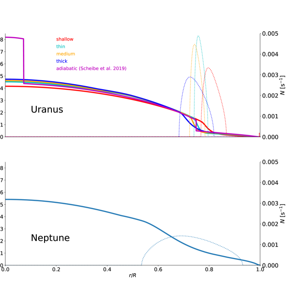
Figure 1: Density (solid lines) and Brunt-Väisälä frequency (dotted) for models of Uranus (top) and Neptune (bottom) as functions of the fractional radius $r/R$. The scales of the $y$-axes are set equal for both the top and bottom panels for easier comparison between Uranus and Neptune models.

The adiabatic normal mode spectrum for a star or planet depends on the profile of mass density $\rho$, adiabatic sound speed $c$, and rotation rate $\Omega$. The adiabatic sound speed $c$ is defined (Unno et al., 1979)

$$c^{2}=\Gamma_{1}\frac{P_{0}}{\rho_{0}},$$ (1)

where $P_{0}$ and $\rho_{0}$ are the pressure and density of the unperturbed state, and the adiabatic exponent $\Gamma_{1}$ is

$$\Gamma_{1}=\left(\frac{\partial\ln P}{\partial\ln\rho}\right)_{\rm{ad}}.$$ (2)

Non-adiabatic regions are characterized by a non-zero Brunt-Väisälä frequency $N$:

$$N^{2}=-\frac{GM_{r}}{r}\left(\frac{d\ln\rho}{d\ln r}-\frac{1}{\Gamma_{1}}\frac{d\ln P}{d\ln r}\right),$$ (3)

where $G$ is the gravitational constant, $M_{r}$ is the mass interior to the radius $r$. For clarity, $M$ without the subscript $r$ will refer to the total mass of the planet. The Brunt-Väisälä frequency $N$ quantifies the angular frequency with which a small parcel of gas oscillates radially with positive or negative buoyancy under local pressure balance with its surrounding gas (Unno et al., 1979).

Here we consider spherically symmetric models so that $\rho=\rho(r)$, $c=c(r)$, and make the further assumption of rigid rotation so that $\Omega(r)=\Omega={\rm constant}$. Although the cloud-level jet streams alone guarantee some degree of differential rotation in Uranus and Neptune (Kaspi et al., 2013), the uncertainty in their underlying bulk rotation rates means that rigidly rotating models are sufficient for our purposes.

The system of equations required to solve for the frequencies of the normal mode spectrum is found in classic works like Unno et al. (1979), and there is now a publicly available and extensively validated asteroseismology software package called GYRE that solves these equations (Townsend & Teitler, 2013). This code has recently been used successfully for Saturn (Mankovich et al., 2019; Markham et al., 2020).

Most models of the interiors of the ice giants make a number of simplifying assumptions, such as a three-layer structure: a rock-rich core, a water-rich envelope, and a hydrogen-rich atmosphere. Many models also assume an adiabatic interior (see, for example, Scheibe et al. 2019). Thermal evolution models, however, suggest that the classical assumption of an adiabatic interior is inconsistent with the luminosities of Uranus and Neptune, and for this reason, models are being explored that are not fully adiabatic, but instead have a thermal boundary layer (see, for example, Scheibe et al. 2021; Stixrude et al. 2021). The gravitational harmonics determined by the Voyager flybys and observations of the dynamics of rings and moons as well as theoretical considerations based on laboratory experiments work together to constrain the properties of the planets’ layers. Some fundamental aspects of ice giant interiors, such as the ice-to-rock mass fraction, are poorly constrained (Helled et al., 2020; Podolak et al., 2019). Even the rotation rates measured by Voyager for Uranus (Desch et al., 1986; Warwick et al., 1986) and Neptune (Warwick et al., 1989) have been called into question (Helled et al., 2010). Given these uncertainties, it is worth considering a relatively broad range of models.

Figure 1 shows profiles of density and Brunt-Väisälä frequency of Uranus and Neptune interior models that we use in this work. What we have labeled the adiabatic model is from Scheibe et al. (2019). Adiabatic oscillation calculations in GYRE require the thermodynamic derivatives $\Gamma_{1}$ (Eq. 2) and

$$\nabla_{\rm ad}=\frac{1}{\Gamma_{1}}\left(\frac{\partial\textrm{ln}T}{\partial\textrm{ln}\rho}\right)_{\rm ad},$$ (4)

which we calculate numerically from the adiabatic model’s $\rho(P)$ and $T(P)$. Because this model assumes a three-layer structure and features density discontinuities owing to sudden composition changes, double mesh points were inserted at the core-envelope and inner-outer envelope boundaries ($r/R\sim 0.07$ and $r/R\sim 0.75$, respectively, where $R$ is the planetary radius) in order for GYRE to apply the appropriate jump conditions at those locations.

We considered a Saturn model from Mankovich & Fuller (2021) and confirmed that our mode calculation reproduced results consistent with theirs, up to the expected error associated with our first-order treatment of rotation (see below).

We have also constructed new models of Uranus and Neptune using the method described in Mankovich & Fuller (2021). In brief, these models are calculated using the fourth-order theory of figures (Nettelmann, 2017), assuming H-He-H₂O mixtures modeled using the MH13-SCvH equation of state for hydrogen and helium (Militzer & Hubbard, 2013; Saumon et al., 1995; Miguel et al., 2016) and Mazevet et al. (2019) for water, combined in an additive-volume approximation. The Mazevet et al. (2019) equation of state for water transitions to that of an ideal gas below $T=800$ K, following Scheibe et al. (2019). Rather than the common practice of imposing discontinuous changes in composition, these models impose a gradient in the water abundance between a homogeneous H-He dominated outer envelope and a homogeneous H₂O-dominated interior. Denoting the H, He and H₂O mass fractions by $X$, $Y$, and $Z$ so that $X+Y+Z=1$, we fix $Y/(X+Y)=0.275$ throughout the model following the protosolar value estimated by Asplund et al. (2009), and for $Z(r)$ assume a sigmoid function with four free parameters specifying the inner and outer radii of the gradient region and the $Z$ values at those boundaries (see Mankovich & Fuller 2021 for details). One of these parameters is eliminated by the condition that the model satisfy each planet’s equatorial radius.

Despite the stabilizing influence of the composition gradient, these models assume for simplicity that temperature is adiabatically stratified, subject to the boundary condition that $T=150$ K at $P=10$ bar, consistent with atmosphere models (Fortney et al., 2011).

We present mode calculations for three Uranus models, one fitting $J_{2}$ and $J_{4}$ exactly, and two that are offset in $J_{4}$ relative to the observed value by approximately $\pm 1$ times the measurement uncertainty $\sigma_{J_{4}}=1.30\times 10^{-6}$ (Jacobson, 2014). The models achieve this by varying the width of the $Z$ gradient region and are accordingly labeled “thin”, “medium” and “thick”, corresponding to $J_{4}$ offsets of $-0.89$, 0, and $+0.79$ times $\sigma_{J_{4}}$, respectively. Another Uranus model we label “shallow” has a $Z$ gradient region closer to the planet’s surface. For Neptune we present a single model that fits $J_{2}$ and $J_{4}$. These models are summarized in Table 3 and their interior structures shown in Figure 1, where the stably stratified composition gradient regions are visible as regions with positive Brunt-Väisälä frequency. Although we are primarily focusing our discussion on f-modes, the models with stably stratified composition regions also generate g-modes, which in principle can mix with the f-modes, and can also be associated with their own resonances.

3.2 Normal Mode Frequency Calculation

Because the ratios of rotation rate to breakup frequency of Uranus and Neptune,

$$\frac{\Omega}{\sqrt{\frac{GM}{R^{3}}}}=\begin{cases}0.175\pm 0.004,&\text{Uranus}\\ 0.155\pm 0.006,&\text{Neptune}\end{cases}$$ (5)

(with uncertainties dominated by uncertainties in the bulk rotation rate; see Desch et al. 1986; Warwick et al. 1986, 1989; Helled et al. 2010), are significant, Coriolis accelerations are not negligible compared to the other terms in the momentum equation. For this reason, the oscillation frequencies given by GYRE are corrected to first order in the planet’s rotation rate $\Omega$ (Ledoux, 1951; Unno et al., 1979). These corrections account for the Doppler shift and the approximate intrinsic perturbation to mode frequencies due to the Coriolis force.

GYRE evaluates an integral to provide the rotation splitting coefficient $\beta$ that is involved in the Coriolis perturbation for solid-body rotation. $\beta$ can also be calculated for a given mode with the equation (cf. Unno et al. 1979)

$$\beta=1-\frac{\int_{0}^{R}\left(2\xi_{r}\xi_{h}+\xi_{h}^{2}\right)\rho r^{2}dr}{\int_{0}^{R}\left[\xi_{r}^{2}+\ell\left(\ell+1\right)\xi_{h}^{2}\right]\rho r^{2}dr}$$ (6)

where $\xi_{r}$ and $\xi_{h}$ are the radial and horizontal components of the displacement eigenfunction (Unno et al., 1979), which is given by

$$\mathbf{\xi}\left(r,\theta,\phi,t\right)= \Biggl{[}\xi_{r}\left(r\right)\hat{r}+\xi_{h}\left(r\right)\left(\hat{\theta}\frac{\partial}{\partial\theta}+\hat{\phi}\frac{1}{\sin\theta}\frac{\partial}{\partial\phi}\right)\Biggr{]}$$ (7)

$$\times Y_{\ell}^{m}\left(\theta,\phi\right)e^{i\sigma_{\ell mn}t},$$

We did verify that the $\beta$ values returned by GYRE are consistent with this formula.

Because Uranus and Neptune rotate more slowly than Jupiter and Saturn, we do not include second-order terms associated with oblateness and the centrifugal force, which together tend to decrease the frequencies (Vorontsov & Zharkov, 1981). For this reason, our uncertainties in calculated mode frequencies, and thus resonance locations, are one-sided.

We calculate the moment of inertia for each model, assuming spherical symmetry, by integrating

$$\frac{I}{MR^{2}}=\frac{8\pi}{3}\frac{\int\rho\left(r\right)r^{4}dr}{MR^{2}}$$ (8)

Table 3 shows the parameters that were used for each model, as well as each model’s calculated moment of inertia.

3.3 Sources of Gravitational Potential Perturbations

Following Marley & Porco (1993), we can write the total gravitational potential as a sum of an unperturbed component and a perturbed component:

$$\Phi=\Phi_{0}+\Phi^{\prime}\left(t\right),$$ (9)

where full expressions for the unperturbed component $\Phi_{0}$ and for the perturbed component $\Phi^{\prime}\left(t\right)$ can be found in Marley & Porco (1993). The integrals for the perturbed gravitational harmonics are taken over the Eulerian density perturbation

$$\rho_{\ell mn}^{\prime}=\rho_{\ell n}^{\prime}\left(r\right)Y_{\ell}^{m}\left(\theta,\phi\right)e^{-i\sigma_{\ell mn}t}$$ (10)

instead of over the unperturbed density $\rho$. In the above equation, $\sigma_{\ell mn}$ is the oscillation frequency in the reference frame that rotates with the planet, $r$ is the radius, $\theta$ is the colatitude, and $\phi$ is the azimuthal angle. The spherical harmonics $Y_{\ell}^{m}$ are defined in terms of the associated Legendre polynomials $P_{\ell}^{m}$.

The equations for the gravitational harmonics that appear in the equations for $\Phi^{\prime}\left(t\right)$ can be reduced to

$$MR^{\ell}J_{\ell n}^{\prime}=-\left(\frac{4\pi}{2\ell+1}\right)^{1/2}e^{i\sigma_{\ell 0n}t}\int_{0}^{R}\rho_{\ell n}^{\prime}\left(r\right)r^{\ell+2}dr$$ (11)

for $m=0$, and

$$MR^{\ell}C_{\ell mn}^{\prime}= \left(-1\right)^{\frac{m+|m|}{2}}\Biggl{[}\frac{2\ell+1}{4\pi}\left(\frac{\left(\ell-|m|\right)!}{\left(\ell+|m|\right)!}\right)\Biggr{]}^{1/2}$$ (12)

$$\times e^{i\sigma_{\ell mn}t}\int_{0}^{R}\rho_{\ell mn}^{\prime}\left(r\right)r^{\ell+2}dr$$

for $m\neq 0$. $S_{\ell mn}^{\prime}$ can be made to vanish by an appropriate choice of phase (Marley & Porco, 1993).

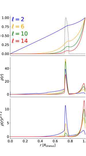
Figure 2: (Top) Radial displacement eigenfunctions for $\ell=2,6,10$, and $14$, normalized to $\xi_{r}=1$ at $r=R$, from the medium Uranus model. The Brunt-Väisälä frequency $N$, normalized to peak at 1, is shown with dotted lines. (Middle) Eulerian density perturbation $\rho^{\prime}\left(r\right)$ for the same four modes. (Bottom) Integrand of Equations 11 and 12, $\rho^{\prime}r^{\ell+2}$, relevant for gravitational potential perturbations, for the same modes. The modes of lower oscillation degree $\ell$ are more sensitive to inner layers of the planet, while the modes of higher oscillation degree $\ell$ are more sensitive to outer layers of the planet.

The radial displacement eigenfunctions of $\ell=2,6,10,$ and $14$ from our medium model are plotted in the top panel of Figure 2, normalized to $\xi_{r}=1$ at $r=R$. We also show the normalized Brunt-Väisälä frequency $N$ as a dotted line to highlight its correlation with the warp in the radial displacement eigenfunctions. The middle panel of Figure 2 shows the Eulerian density perturbation of the same modes $\ell=2,6,10,$ and $14$. The bottom panel of Figure 2 shows the integrand of Equations 11 and 12, $\rho^{\prime}r^{\ell+2}$, for each of these modes. These plots illustrate how the modes of lower spherical harmonic degree $\ell$ can probe deeper into the planet, whereas the modes of higher spherical harmonic degree $\ell$ are more sensitive to the outer layers and to the parts of the planet that are stably stratified.

Only the spherical harmonic $Y_{\ell}^{0}$ contributes to the $J_{\ell n}^{\prime}$ term due to the orthogonality of the spherical harmonics. Likewise, for $m\neq 0$, the contribution to each $C_{\ell mn}^{\prime}$ term is only from the $Y_{\ell}^{m}$ harmonic. Each oscillation mode thus contributes to a single perturbed gravitational harmonic. The planet’s rotation, however, can mix modes slightly. For Saturn, no more than 15% of the rotationally corrected radial displacement eigenfunction could be attributed to mode mixing (Marley & Porco, 1993); for Uranus and Neptune, which rotate more slowly than Saturn, we can expect mode mixing to influence the radial displacement eigenfunction to an even lesser extent.

3.4 Resonance Calculation

We calculate the pattern frequency $\Omega_{\rm{pat}}$ of each normal mode seen from inertial space,

$$\Omega_{\rm{pat}}=\frac{1}{m}\left(\sigma_{\ell n}^{0}+m\beta\Omega\right),$$ (13)

where $\sigma_{\ell n}^{0}$ is the oscillation frequency in the non-rotating limit for the mode specified by $\ell$ and $n$, and $\beta$ is the rotation splitting coefficient defined in Equation 6. Our models for Uranus assume the rotation rate provided in Helled et al. (2010), called the fast rotation rate, corresponding to a period of 16.58 hours. The adiabatic model assumes the classical, or slow, rotation rate, corresponding to a period of 17.24 hours (Desch et al., 1986; Warwick et al., 1986). Our Neptune model likewise uses the rotation rate from Helled et al. (2010), corresponding to a period of 17.46 hours, which in contrast is slower than the classical rotation rate provided by Voyager 2 radio data, corresponding to a period of 16.11 hours (Warwick et al., 1989). In general, resonance locations of a faster rotator fall further inward than those of a slower rotator. Thus the rotation rate of these planets is another parameter that ring seismology could help constrain, similar to how Mankovich et al. (2019) calculated a seismological rotation rate for Saturn.

model	$R$ (km)	$M$ ($\times 10^{25}$ kg)	$\Omega$ ($\times 10^{-4}$ s-1)	$J_{2}$ ($\times 10^{-4}$)	$J_{4}$ ($\times 10^{-4}$)	$I/MR^{2}$
Uranus shallow	25,559	8.68009	1.0527	35.1068	-0.341705	0.2279
Uranus thin	25,559	8.68009	1.0527	35.1068	-0.330171	0.2204
Uranus medium	25,559	8.68009	1.0527	35.1068	-0.341705	0.2202
Uranus thick	25,559	8.68009	1.0527	35.1069	-0.351949	0.2200
Uranus adiabatic†	25,559	8.68009	1.0124	35.107	-0.342	0.2266
Neptune	24,764	10.24092	0.9996	34.0843	-0.334	0.2509

Table 3: Parameters of the planetary models. Equatorial radii $R$ are from Archinal et al. (2018). $M$, $J_{2}$, and $J_{4}$ of Uranus are from Jacobson (2014), while $M$, $J_{2}$, and $J_{4}$ of Neptune are from Jacobson (2009). The classical Uranus spin rate $\Omega$ is from Voyager 2 radio data (Desch et al., 1986; Warwick et al., 1986) and is used only in the adiabatic model, while alternate spin rates $\Omega$ based on the shapes and gravitational coefficients of the planets are from Helled et al. (2010) and are used in the other models. The classical Neptune spin rate $\Omega$, not used in any of our models, is $1.0834\times 10^{-4}$ s^-1 (Warwick et al., 1989). The moments of inertia are calculated using Equation 8.
^† Scheibe et al. (2019)

Then we calculate the resonance location numerically. Lindblad resonances occur at locations where the following relationship is satisfied (Goldreich & Tremaine, 1979):

$$m\left(n-\Omega_{\rm{pat}}\right)=\pm q\kappa,$$ (14)

where the upper sign corresponds to an inner Lindblad resonance and the lower sign corresponds to an outer Lindblad resonance, $q$ is a positive integer, and $n$ and $\kappa$ are the resonance location’s mean motion and horizontal epicyclic frequency, respectively. These are calculated according to the second-order equations from Renner & Sicardy (2006).

Similarly, vertical resonances occur at locations where

$$m\left(n-\Omega_{\rm{pat}}\right)=\pm b\mu,$$ (15)

where the upper sign corresponds to an inner vertical resonance and the lower sign corresponds to an outer vertical resonance, $b$ is a positive integer, and $\mu$ is the resonance location’s vertical epicyclic frequency, which is found using the equation from Shu et al. (1983):

$$\mu^{2}+\kappa^{2}=2n^{2}$$ (16)

We are focusing only on first-order resonances, which have $q=b=1$, though higher-order resonances are possible (Marley, 2014).

Corotation resonances are potentially interesting to consider in the context of Neptune’s Adams ring (see Section 5.4). Hence we compute corotation resonance locations for Neptune following the same procedures as in A’Hearn et al. (2021). That is, we find the radii where the mean motion $n$ matches the pattern frequencies $\Omega_{\rm{pat}}$ associated with the $\ell=m$ modes we have calculated from our Neptune model.

4 Results

Figures 3 and 4 show the calculated resonance locations with f-mode oscillations for all our Uranus models. Figure 3 shows the Lindblad resonances, while Figure 4 shows the vertical resonances. We show the resonance locations up to $\ell=25$. For every mode, the resonance location of the medium model falls in between those of the thin and thick models. The resonance location of the thick model typically falls further outward (and the resonance location of the thin model falls further inward), the $\ell=m=2$ mode being the sole exception. This general trend is set by the models’ different predictions for density in the outer envelope, which the higher $m$ modes are more sensitive to (cf. Figure 2).

The region of particular interest that we find spans from the $6$ ring to the $\beta$ ring. Satellite resonances do not line up with these inner rings (Hedman & Chancia, 2021), but several high-$m$ mode resonances from our models do fall in this region. The predictions from our models as well as from Marley et al. (1988) include resonance locations that fall in the $\zeta$ ring for the modes with $\ell\leq 5$. The $\zeta$ ring, however, has low optical depth, and would not be expected to sustain a wave.

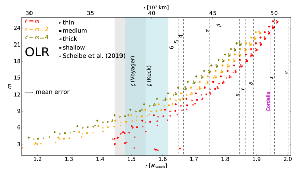
Figure 3: Normal mode outer Lindblad resonance (OLR) location predictions from all five Uranus models. The azimuthal order $m$ (equivalent to the number of spiral arms) is the vertical axis, and distance from the center of Uranus is the horizontal axis, shown in Uranus radii on the bottom and in km on the top. OLRs can excite inward-propagating spiral density waves. The typical uncertainty of these resonance locations is shown by one bar on the left.

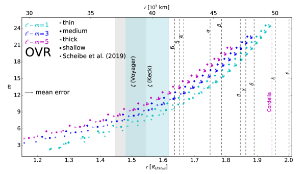
Figure 4: Normal mode outer vertical resonance (OVR) location predictions from all five Uranus models. The azimuthal order $m$ (equivalent to the number of spiral arms) is the vertical axis, and distance from the center of Uranus is the horizontal axis, shown in Uranus radii on the bottom and in km on the top. OVRs can excite outward-propagating bending waves. The typical uncertainty of these resonance locations is shown by one bar on the left.

Lindblad resonances that fall among the inner rings are listed in Table 4, whereas vertical resonances are listed in Table 5. The resonance locations are given in general ranges, based on all our models as well as the frequency uncertainty from our calculations with first-order rotation corrections. Predictions based on individual interior models are found in the Appendices. We group the 6, 5, and 4 rings together, and the $\alpha$ and $\beta$ rings together, in these tables, because the uncertainty associated with a mode’s frequency or resonance location is comparable to the distance between these narrow rings. Differential rotation confined to the outer layers of the interior will have a greater effect on the higher-degree modes.

Among the 6, 5, and 4 rings, we expect that a Lindblad resonance with $m=2$ or $7\leq m\leq 13$, or a vertical resonance with $9\leq m\leq 14$, could be from a planetary normal mode. Among the $\alpha$ and $\beta$ rings, we expect that a Lindblad resonance with $11\leq m\leq 18$, or a vertical resonance with $13\leq m\leq 19$, could be from a planetary normal mode.

$\ell$	$m$	$\Omega_{\rm{pat}}$ (deg/day)	$r_{\rm{res}}$ (km)
6, 5, or 4 ring		41,838; 42,235; 42,572
2	2	1995.2-2360.4	38571-43142
7	7	1585.4-1753.2	39244-41963
8	8	1517.2-1666.7	40166-42760
9	9	1460.4-1591.0	41088-43498
10	10	1412.3-1525.1	41981-44184
12	10	1506.0-1605.7	40565-42334
13	11	1450.1-1537.1	41532-43175
14	12	1402.8-1479.3	42409-43935
16	12	1466.5-1537.2	41338-42655
17	13	1419.4-1482.8	42176-43420
$\alpha$ or $\beta$ ring		44,719; 45,661
11	11	1370.9-1467.8	42827-44822
12	12	1334.6-1418.1	43618-45417
13	13	1301.1-1375.0	44350-46012
14	14	1271.6-1337.3	45024-46562
15	15	1245.4-1304.3	45644-47070
16	14	1326.8-1387.5	43933-45262
17	15	1295.6-1350.5	44598-45850
18	16	1267.7-1318.0	45211-46397
19	15	1342.5-1395.1	43644-44776
20	16	1310.5-1359.2	44294-45382
21	17	1281.9-1327.2	44897-45949
22	18	1256.1-1298.6	45460-46480

Table 4: Predicted Lindblad resonance locations among the inner rings of Uranus. The ranges in frequencies and locations take into account the two most extreme models and include the error in the range given.

$\ell$	$m$	$\Omega_{\rm{pat}}$ (deg/day)	$r_{\rm{res}}$ (km)
6, 5, or 4 ring		41,838; 42,235; 42,572
10	9	1517.1-1642.0	40245-42420
11	10	1460.6-1566.9	41241-43216
12	11	1412.5-1503.4	42159-43945
14	11	1486.3-1569.6	40966-42481
15	12	1435.2-1508.5	41868-43281
17	12	1496.8-1565.4	40850-42086
18	13	1446.7-1508.4	41704-42882
19	14	1403.1-1459.4	42486-43614
$\alpha$ or $\beta$ ring		44,719; 45,661
14	13	1332.1-1402.8	43769-45302
15	14	1299.6-1362.7	44471-45896
16	15	1270.9-1327.7	45115-46446
18	15	1319.4-1373.0	44117-45303
19	16	1289.4-1338.8	44748-45881
20	17	1262.6-1308.4	45333-46422
21	16	1331.0-1379.2	43872-44922
22	17	1300.7-1345.8	44491-45511
23	18	1273.4-1315.8	45069-46063
24	19	1248.7-1288.8	45612-46582

Table 5: Predicted vertical resonance locations near the inner rings of Uranus.

Although planetary normal mode resonances with $m>15$ may fall among the $\eta$, $\gamma$, $\delta$, $\lambda$, and $\epsilon$ rings, we expect the dynamics of these rings to be influenced more by the moons Cordelia and Ophelia. The case has been made that while Cordelia is the outer shepherd of the $\delta$ ring and the inner shepherd of the $\epsilon$ ring, Ophelia is the outer shepherd of both the $\epsilon$ and $\gamma$ rings (Porco & Goldreich, 1987). Recently, the $\eta$ ring was found to be influenced by Cressida (Chancia et al., 2017). Nevertheless, at Saturn the $\ell=m=10$ mode was found to be anomalously strong (Hedman et al., 2019), and with this precedent the influence of planetary normal modes on the outer rings cannot be ruled out.

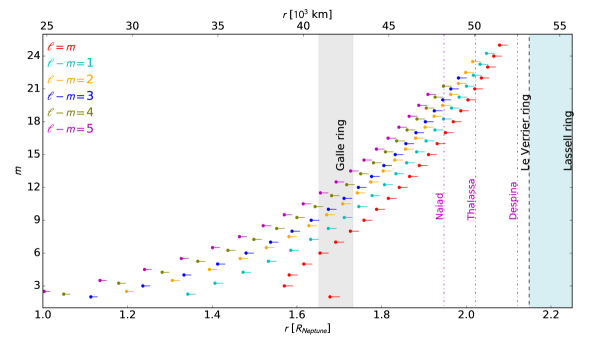
Figure 5: Normal mode resonance location predictions for Neptune. The azimuthal order $m$ is the vertical axis, and distance from the center of Neptune is the horizontal axis, shown in Neptune radii on the bottom and in km on the top. Both outer Lindblad resonances (OLR) and outer vertical resonances (OVR) are shown. Several resonances fall in the Galle ring, and others may perturb the inner moons Naiad and Thalassa.

At Neptune, modes with $\ell=m=16,...,21$ fall among the moons Naiad and Thalassa. Naiad and Thalassa are themselves in a 73:69 resonance (Brozović et al., 2020), made possible by Naiad’s high inclination (4.7^∘). Should it be found that this resonance does not fully account for their orbits, perturbations from planetary normal modes may be part of the solution. Furthermore, it is not known how Naiad reached its high inclination. The most likely explanation is passage through a previous resonance with Despina (Banfield & Murray, 1992). Another possibility, however, is that Naiad’s inclination was excited instead by a vertical resonance with a Neptunian normal mode.

The above calculations focused exclusively on the f-modes ($n=0$). It is also interesting, however, to consider the $\ell=m$, $n=1$ g-modes for the non-adiabatic models because these can also fall among the ring systems. In the Uranian system (Figure 6), $\ell=m$, $n=1$ g-mode resonances are likely to fall in the mid- to outer-ring system as well as the innermost moons. The spread in resonance location predictions is greater for g-modes than for f-modes because the g-mode spectrum is sensitive mainly to the Brunt-Väisälä frequency $N(r)$. The thin-medium-thick triplet of models diverges more for higher $\ell$, where the eigenfunctions have higher amplitudes in the g-mode cavity.

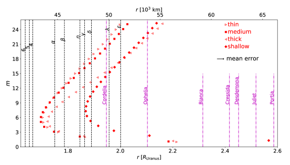
Figure 6: Resonance location predictions for Uranian g-modes. The azimuthal order $m$ is the vertical axis, and distance from the center of Uranus is the horizontal axis, shown in Uranus radii on the bottom and in km on the top. Only outer Lindblad resonances (OLR) with $\ell=m$, $n=1$ are shown.

In the Neptunian system (Figure 7), $\ell=m$, $n=1$ g-mode resonances are likely to fall among the inner moons and middle to outer rings. There is even a g-mode resonance that falls near the Adams ring, which we discuss in Section 5.4. G-modes at higher order ($n\geq 2$) are at lower frequency, and so their outer Lindblad resonance locations would fall farther out. Nevertheless, their gravity perturbations might be too small to matter because they are more effectively confined deep down than the $n=1$ g-modes.

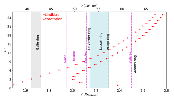
Figure 7: Resonance location predictions for Neptunian g-modes. The azimuthal order $m$ is the vertical axis, and distance from the center of Neptune is the horizontal axis, shown in Neptune radii on the bottom and in km on the top. Outer Lindblad resonances (OLR) with $\ell=m$, $n=1$ are shown as filled-in circles, while corotation resonances associated with these Lindblad resonances are shown with open circles.

Note that the mean absolute model uncertainty, due to the approximate treatment of rotation, in the resonance locations for all the f-modes we calculated is $\delta r=610$ km for the Uranus models and $\delta r=450$ km for the Neptune model. The maximum uncertainty in f-mode resonance locations is $\delta r=805$ km for the Uranus models and $\delta r=557$ km for the Neptune model. These both correspond to the $\ell=m=2$ f-mode. The uncertainty generally decreases with increasing $m$.

To decrease the uncertainty, frequency-correction calculations may be carried out to second-order using the perturbation theory techniques described in Vorontsov & Zharkov (1981) and summarized in the Appendix of Marley (1990). We leave the second-order calculations for possible future work. Further knowledge of the planets’ interior structure, thermodynamic state, and rotational state can also improve the precision of resonance location predictions.

5 Discussion

We have found that planetary normal modes likely fall among the rings of Uranus and Neptune. The next question is whether normal mode resonances would be detectable in the Uranian and Neptunian rings. Potential signatures of such resonances could include wave-like structures in the dense Uranian rings, correlations with Uranus’s many narrow ring features, and longitudinal structures in more dusty rings. Each of these methods is discussed in more detail below.

Note that we do not attempt to compute the explicit amplitudes of the gravitational perturbations associated with these perturbations. While Marley & Porco (1993) estimated the strengths of the perturbations needed to produce the observed waves in Saturn’s rings, more recent kronoseismology studies did not find strong correlations between the anticipated and the observed amplitudes of normal mode resonances (Hedman et al., 2019). Although it is expected that torques decrease as the oscillation degree $\ell$ increases because a smaller quantity of mass participates in the oscillation (Marley & Porco, 1993), the intrinsic amplitude spectrum of normal modes in the planet is unknown but the subject of much current research (Marley & Porco, 1993; Markham & Stevenson, 2018; Wu & Lithwick, 2019; Markham et al., 2020). For example, Markham & Stevenson (2018) examined mode excitation mechanisms in giant planet interiors. They found that moist convective storms associated with water condensation were not energetically feasible for Jupiter, but it remains to be seen whether that mechanism could excite Uranian or Neptunian modes to observable levels. Given all these theoretical uncertainties, we leave the computation of amplitudes for future work.

5.1 Occultations of Narrow Dense Rings

One way to identify resonant perturbations would be the detection of density waves similar to those seen in Saturn’s rings. This would best work in Uranus’s narrow dense rings, where the search can be guided by a combination of our location predictions and the range of the number of spiral arms $m$ corresponding to an approximation of the number of stellar occultation cuts through the rings or images of the rings that would be necessary for detection. Note that the resolution achievable with an occultation is limited by the Fresnel scale: $\lambda_{F}\sim\sqrt{\lambda D}$. At $\lambda=0.2\mu$m, the great distances $D$ of Uranus (19.2 AU) and Neptune (30 AU) from Earth prevent ground-based or Earth-orbit-based stellar occultations from obtaining better resolution than about 750 m and 950 m, respectively. Given that wave-like variations in the dense rings have sub-kilometer wavelengths (Chancia & Hedman, 2016; Horn et al., 1988), we expect resolutions of order 200 m is needed to see any planet-generated waves. This resolution threshold, combined with the number of cuts required to uniquely determine the number of arms, which is of order the relevant $m$ (about 20 for the waves of interest here), implies that the detection of planetary normal modes via wave identification will have to await an orbiter of Uranus or Neptune. An orbiter can observe occultations in the ultraviolet, visible, near-infrared, and radio parts of the spectrum at a much closer distance, and it would be expected to produce radial profiles of the rings at a range of longitudes with sufficient resolution to determine the number of spiral arms in a wave. Observation of the ring plane from different incidence angles will also allow bending waves to be easily discerned from density waves.

While the overall shapes of the Uranian rings are dominated by factors that can be attributed to free modes in the rings themselves, this does not exclude the possibility that these rings can also preserve signals from planetary normal modes. The Uranian $\alpha$ and $\beta$ rings are considered analogs of the Saturnian Maxwell and Colombo ringlets (Porco, 1990; Chiang & Culter, 2003). These rings are considered in Chiang & Culter (2003), who present a proof, relying on first steps taken by Borderies et al. (1983), that circular, nodally locked rings are linearly stable to perturbations to their inclinations and nodes. The Colombo ringlet, also named the Titan ringlet because it is in a 1:0 apsidal resonance with Saturn’s moon Titan (Porco et al., 1984; Nicholson et al., 2014), is located near several planetary normal modes: $6\leq\ell\leq 15$, $5\leq m\leq 11$ (Mankovich et al., 2019). The Maxwell ringlet inside the Maxwell Gap in Saturn’s C ring is perturbed by an $\ell=m=2$ mode (French et al., 2016; Cuzzi et al., 2018), as predicted by Fuller (2014). For this reason, we are also hopeful that either the $\alpha$ or $\beta$ rings, or both, are likewise perturbed by planetary normal modes. The Uranian $\epsilon$ ring is also considered to have similar properties to the Maxwell ringlet (French et al., 1991, 2016): sharp edges, a freely precessing elliptical shape, and a linear width-radius relation. The mean optical depth of the Maxwell ringlet is $\bar{\tau}=0.968$ (French et al., 2016).

Horn et al. (1988) identified an inward-propagating density wave in the $\delta$ ring, which they interpreted to be evidence of a moonlet interior to the $\delta$ ring. Because no moonlet has yet been discovered interior to the $\delta$ ring, we consider that such a density wave could be a candidate planetary normal mode resonance. Horn et al. (1988) constrained the azimuthal wavenumber $m$ of the resonance that generated this wave to be $48\leq m\leq 112$, based on three conditions: that the torque exceed a critical value (Goldreich & Porco, 1987) for nonlinearity and the moonlet still remain undetected in the Voyager Imaging search (Smith et al., 1986), that the moonlet lie between the $\gamma$ and $\delta$ rings, and that the separation in radius between first-order resonances be greater than half the width of the $\delta$ ring (Horn et al., 1988). The range of possible $m$ values was thus not constrained by an $m$-lobed pattern detected in the ring itself. If instead the inward-propagating density wave in the $\delta$ ring is driven by a planetary normal mode resonance, none of the conditions given by Horn et al. (1988) would apply, though their measurement of the product of the wavelength and the distance from the resonance $\lambda d=0.84\pm 0.07$ km (Horn et al., 1988) makes it difficult for $m$ to be less than 10. From our resonance location predictions, we can instead expect $17\leq m\leq 23$, should the density wave in the $\delta$ ring be from an f-mode resonance.

In addition to density waves, Lindblad resonances with satellites can perturb ring edges, generating non-circular shapes like those observed for the outer edge of Saturn’s A and B rings (Goldreich & Tremaine, 1978; Nicholson et al., 2014; El Moutamid et al., 2016; Tajeddine et al., 2017) and for Uranus’s $\epsilon$ ring (French et al., 1991) and $\eta$ ring (Chancia et al., 2017).

5.2 Correlating Uranian Ring Features and Resonance Locations

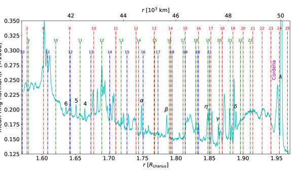
Figure 8: Radial scan of Uranian rings compared to Lindblad resonance predictions from the medium model. The cyan curve shows the mean ring normal $I/F$ as a function of radius. While the named narrow rings are labeled, many other narrow features can be seen in this scan. The tallest dash-dotted lines, in red, show the locations of the $\ell=m$ mode resonances; the intermediate-sized dash-dotted lines, in green, show the locations of the $\ell-m=2$ mode resonances, and the shortest dash-dotted lines, in blue, show the locations of the $\ell-m=4$ mode resonances. The integer above each dash-dotted line corresponds to the azimuthal order $m$ of the mode.

Another potential way to identify these resonances would be to correlate the locations of multiple narrow ring features with expected resonant locations. For example, Figure 8 shows the brightness of the inner rings of Uranus as a function of radius, from a high-phase image (C2685219; see Hedman & Chancia 2021) that showed many more narrow ring features than the named rings. These features could potentially reflect additional locations where material is confined by resonances. Vertical dash-dotted lines show Lindblad resonance locations calculated from the medium model. Due to the uncertainty of our calculations, lining up ring features with resonances in this way is to be taken only as a demonstration of a way to correlate the models with ring features. Nevertheless, the way that the $\ell=m=8,9,10,11,12$ modes line up with either peaks or troughs in the ring brightness is suggestive of a role they may play in perturbing ring material radially.

5.3 Longitudinal Variations in Diffuse Rings

The Uranian $\zeta$ ring and the Neptunian Galle ring have low optical depth. Although many mode resonances fall within them, these rings are so tenuous that we do not expect them to be capable of sustaining a wave. Longitudinal structure can be driven by resonances with the planet’s magnetic field, as is the case at magnetic Lindblad resonances in Saturn’s D Ring (Hedman et al., 2009a; Chancia et al., 2019), and we encourage future work exploring potential resonances between the Uranian and Neptunian magnetic fields and their ring systems. Nonetheless, planetary normal modes, particularly the stronger $\ell=m=2$ modes, should be kept in mind in studies of longitudinal structures in diffuse rings.

5.4 Neptune’s Le Verrier and Adams Rings

Finally, we can consider whether planetary normal mode resonances could influence the dynamics of Neptune’s narrow dusty rings in a detectable way.

While normal mode resonances could potentially play a role in confining the Le Verrier ring (Brooks et al., 2021), testing this idea is challenging. For one, the ring appears homogeneous in the Voyager images (Ferrari & Brahic, 1994), which limits our ability to identify signatures of external perturbations. Furthermore, this ring is also close to other resonances, including Thalassa’s 21:23 resonance (Gaslac Gallardo et al., 2020). In addition, the 2:1 resonance with Neptune’s rotation frequency, whose value is known with less certainty, falls in the Le Verrier ring region. Simply applying Kepler’s Third Law to find the 2:1 resonance location, neglecting Neptune’s oblateness, yields

$$a_{\rm{res}}=\left(\frac{GM}{n^{2}}\right)^{1/3}=\begin{cases}52,607\>\rm{km},&\text{fast}\\ 55,507\>\rm{km},&\text{slow}\end{cases}$$ (17)

where the mean motion $n=2\Omega$, and “fast” and “slow” refer to estimates for Neptune’s rotation rate given in Table 3. The Le Verrier ring is located at 53,200 km (de Pater et al., 2018), in the middle of the resonance locations according to the two different rotation rates (Warwick et al., 1989; Helled et al., 2010).

It is also worth noting that $n=1$ g-mode resonances can occur near Neptune’s Adams ring, because this could potentially mean that these resonances may be relevant to understanding the arcs in that ring. The ring arcs in the Adams ring comprise the most studied part of Neptune’s rings (see for example Porco et al. 1995; de Pater et al. 2018). Ring arcs in the Saturnian system are confined longitudinally by orbital resonances with moons (Spitale et al., 2006; Hedman et al., 2007, 2009b, 2010; Cooper et al., 2008; A’Hearn et al., 2019). Although several ideas have been proposed about the particular resonance of Neptune’s ring arcs, consensus has not been reached. Initial studies suspected that a 42:43 resonance with Galatea confined the ring arcs (Goldreich et al., 1986; Porco, 1991; Namouni & Porco, 2002). Deviations from the exact rate of different types of a corotation resonance with Galatea, however, support other possible explanations (Renner et al., 2014). Confinement due to shepherding by undetected satellites that are co-orbital with the Adams ring arcs has been proposed (Lissauer, 1985; Salo & Hanninen, 1998; Renner et al., 2014), though more recent investigation claims to rule out that co-orbital satellites could be the source of the dust (Giuliatti Winter et al., 2020). Another recent idea is that the Adams ring arcs are in a three-body resonance with Galatea and Larissa (Showalter et al., 2017).

One potential way to test whether planetary normal modes could be confining material in the Adams ring is to take another look at the distribution and extent of the arcs. A consequence of the initial 42:43 corotation resonance theory of confinement was that each of the 42 corotation sites, also called “pockets”, spans only $\sim 9^{\circ}$. This posed a problem for the Fraternité arc, whose longitudinal extent is greater, and so it was assumed that Fraternité occupies two corotation sites.

Should the ring arcs instead be the effect of a corotation resonance with an oscillation degree $m<42$ , the corotation site would span a greater longitudinal extent $\theta$, because

$$\theta=\frac{360^{\circ}}{m},$$ (18)

which for low enough $m$ could encompass the entirety of Fraternité in one corotation site. Although Lindblad resonances do not confine material, each Lindblad resonance can be associated with a corotation resonance, which can confine material. The planetary corotation resonance from the $\ell=m=19$, $n=1$ g-mode is calculated to fall in the range $62,844$-$63,230$ km, which encompasses the Adams ring. The $m=19$ corotation site would span approximately $19^{\circ}$, over twice as much as an $m=42$ corotation site, and could thus encompass the entirety of the Fraternité arc. We hope to explore this possibility further in a future work.

5.5 Conclusion

While none of the structures in the rings around Uranus and Neptune has yet been firmly attributed to a planetary normal mode, the above considerations indicate that ring seismology of the ice giants could be done when the appropriate data becomes available. To the extent that different interior models affect normal mode resonance locations, the detection of planet-driven ring waves or perturbations to moon orbits would allow a variety of interior models to be ruled out. These may provide evidence for or against a stably stratified layer or a diffuse core. Stable stratification, which occurs in all our interior models except the adiabatic model, allows the presence of g-modes, which could possibly be detected if they fall in or near rings (Fuller, 2014; Friedson, 2020). Should Uranus or Neptune additionally have a diffuse core, for example, the f-mode and g-mode resonances would be modified compared to our results here, particularly those corresponding to the $\ell=2$ modes most sensitive to $\rho(r)$ and $N(r)$ in the deep interior.

To evaluate these predictions, attempts can be made with Voyager and ground-based observations. Nevertheless, we expect results from such observations to be inconclusive, and an orbiter with a primary mission duration of at least a year or two to measure pattern speeds to within around $0.1^{\circ}$/day would likely be required to make the observations necessary to determine effects from planetary normal mode resonances in the rings of Uranus and Neptune.

We are grateful to many individuals for useful comments and discussions, including P. Nicholson, M. Tiscareno, M. Ćuk, L. Fletcher, M. Brozović, and K. Volk. We thank two anonymous reviewers for their helpful comments that have improved this paper. We also thank NASA for the support through the Solar System Workings grants NNX15AH45G and 80NSSC21K1865.

Appendix A Extended Tables of f-mode Frequencies and Resonance Locations

In this appendix, we present all the calculated f-mode frequencies and resonance locations for all the models. Table 6 shows the initial estimates by Marley et al. (1988). Our Lindblad resonance calculations are provided in tables that contains two models each: the thick and medium models in Table 7, the thin and adiabatic models in Table 8, and the shallow and Neptune models in Table 9. Similarly, our vertical resonance calculations are then provided in tables that contains two models each: the thick and medium models in Table 10, the thin and adiabatic models in Table 11, and the shallow and Neptune models in Table 12. Error bars are one-sided because the frequencies and resonance locations are only calculated to first order. Second-order calculations would universally lower the frequencies, which would cause the resonance locations to be more distant from the planet.

Table 6: Predicted Lindblad resonance locations among the inner rings of Uranus from Marley et al. (1988).

$\ell$	$m$	model	$\Omega_{\rm{pat}}$ (deg/day)	$r_{\rm{res}}$ (km)
2	2	6	1683	48,300
		5	1718	47,700
		4	1767	46,800
3	3	6	2015	39,600
		5	2025	39,500
		4	2054	39,100
4	4	6	2005	38,100
		5	2010	38,000
		4	2030	37,800
5	5	6	1941	37,900
		5	1941	37,900
		4	1950	37,800

Table 7: Pattern frequencies and Lindblad resonance locations of different models

Uranus Thick model
$\ell$	$m$	$\Omega_{\rm{pat}}$ (deg/day)	$r_{\rm{res}}$ (km)
$\ell=m$
2	2	2218.7 - 62.4	40196 + 772
3	3	2228.9 - 59.9	37054 + 678
4	4	2077.7 - 53.6	37198 + 653
5	5	1922.5 - 47.8	38123 + 644
6	6	1788.3 - 42.9	39263 + 641
7	7	1677.2 - 39.1	40418 + 639
8	8	1586.7 - 35.9	41503 + 638
9	9	1513.3 - 33.4	42481 + 636
10	10	1453.5 - 31.4	43345 + 634
11	11	1404.4 - 29.7	44106 + 632
12	12	1363.3 - 28.3	44780 + 629
13	13	1328.1 - 27.0	45386 + 626
14	14	1297.5 - 26.0	45939 + 623
15	15	1270.5 - 25.0	46451 + 620
16	16	1246.2 - 24.2	46928 + 617
17	17	1224.3 - 23.4	47377 + 614
18	18	1204.3 - 22.7	47802 + 611
19	19	1185.9 - 22.1	48205 + 608
20	20	1169.0 - 21.5	48589 + 605
21	21	1153.2 - 21.0	48955 + 602
22	22	1138.6 - 20.5	49305 + 600
23	23	1125.0 - 20.0	49640 + 597
24	24	1112.2 - 19.6	49962 + 594
25	25	1100.2 - 19.2	50271 + 592
$\ell-m=2$
4	2	3755.8 - 107.2	28306 + 551
5	3	2919.8 - 79.6	30955 + 575
6	4	2460.7 - 64.4	33234 + 592
7	5	2166.4 - 54.7	35208 + 604
8	6	1961.7 - 47.9	36916 + 613
9	7	1812.2 - 43.0	38388 + 618
10	8	1699.1 - 39.2	39654 + 621
11	9	1610.9 - 36.3	40749 + 623
12	10	1540.2 - 33.9	41705 + 623
13	11	1482.1 - 32.0	42553 + 622
14	12	1433.1 - 30.3	43314 + 621
15	13	1391.1 - 28.9	44007 + 619
16	14	1354.5 - 27.6	44644 + 617
17	15	1322.1 - 26.6	45234 + 615
18	16	1293.3 - 25.6	45784 + 613
19	17	1267.3 - 24.7	46299 + 611
20	18	1243.8 - 23.9	46784 + 609
21	19	1222.4 - 23.2	47242 + 606
22	20	1202.7 - 22.5	47675 + 604
23	21	1184.6 - 21.9	48087 + 602
24	22	1167.9 - 21.3	48478 + 599
25	23	1152.3 - 20.8	48852 + 597
$\ell-m=4$
7	3	3307.8 - 91.1	28487 + 535
8	4	2711.8 - 71.9	31153 + 562
9	5	2350.3 - 60.1	33349 + 581
10	6	2108.3 - 52.3	35187 + 593
11	7	1935.4 - 46.6	36743 + 602
12	8	1805.6 - 42.4	38080 + 607
13	9	1704.4 - 39.1	39246 + 610
14	10	1622.9 - 36.4	40278 + 612
15	11	1555.6 - 34.1	41203 + 613
16	12	1498.8 - 32.3	42041 + 614
17	13	1450.1 - 30.6	42807 + 613
18	14	1407.7 - 29.2	43512 + 612
19	15	1370.5 - 28.0	44165 + 611
20	16	1337.4 - 26.9	44772 + 610
21	17	1307.8 - 25.9	45340 + 608
22	18	1281.1 - 25.0	45873 + 607
23	19	1256.9 - 24.2	46375 + 605
24	20	1234.7 - 23.5	46849 + 603
25	21	1214.4 - 22.8	47298 + 601

Uranus Medium model
$\ell$	$m$	$\Omega_{\rm{pat}}$ (deg/day)	$r_{\rm{res}}$ (km)
$\ell=m$
2	2	2207.8 - 62.1	40328 + 774
3	3	2234.6 - 60.1	36991 + 678
4	4	2096.0 - 54.2	36981 + 651
5	5	1949.2 - 48.6	37774 + 641
6	6	1819.6 - 43.9	38812 + 636
7	7	1710.1 - 40.0	39899 + 634
8	8	1618.6 - 36.8	40956 + 632
9	9	1542.1 - 34.2	41951 + 630
10	10	1477.8 - 32.0	42870 + 629
11	11	1423.3 - 30.1	43714 + 627
12	12	1377.0 - 28.6	44481 + 626
13	13	1337.5 - 27.3	45174 + 624
14	14	1303.6 - 26.1	45797 + 621
15	15	1274.3 - 25.1	46358 + 619
16	16	1248.7 - 24.3	46867 + 616
17	17	1226.0 - 23.5	47335 + 614
18	18	1205.5 - 22.8	47771 + 611
19	19	1186.8 - 22.1	48180 + 608
20	20	1169.7 - 21.5	48568 + 605
21	21	1153.9 - 21.0	48937 + 602
22	22	1139.2 - 20.5	49289 + 600
23	23	1125.4 - 20.0	49626 + 597
24	24	1112.6 - 19.6	49949 + 594
25	25	1100.5 - 19.2	50259 + 592
$\ell-m=2$
4	2	3792.6 - 108.4	28123 + 548
5	3	2963.8 - 81.0	30649 + 571
6	4	2506.6 - 65.8	32828 + 587
7	5	2210.9 - 56.0	34735 + 598
8	6	2002.6 - 49.1	36413 + 606
9	7	1847.7 - 43.9	37895 + 612
10	8	1728.0 - 40.0	39211 + 616
11	9	1633.0 - 36.8	40381 + 618
12	10	1556.0 - 34.3	41424 + 619
13	11	1492.6 - 32.2	42352 + 620
14	12	1439.9 - 30.5	43178 + 619
15	13	1395.4 - 29.0	43917 + 618
16	14	1357.2 - 27.7	44584 + 617
17	15	1324.0 - 26.6	45192 + 615
18	16	1294.6 - 25.6	45753 + 613
19	17	1268.4 - 24.7	46275 + 611
20	18	1244.6 - 23.9	46764 + 609
21	19	1223.1 - 23.2	47224 + 606
22	20	1203.3 - 22.5	47660 + 604
23	21	1185.1 - 21.9	48073 + 602
24	22	1168.3 - 21.4	48466 + 599
25	23	1152.7 - 20.8	48840 + 597
$\ell-m=4$
7	3	3379.5 - 93.3	28084 + 528
8	4	2770.6 - 73.6	30711 + 555
9	5	2397.7 - 61.5	32909 + 574
10	6	2145.0 - 53.3	34785 + 587
11	7	1962.4 - 47.3	36406 + 597
12	8	1824.4 - 42.9	37819 + 603
13	9	1716.8 - 39.4	39058 + 608
14	10	1630.7 - 36.6	40150 + 611
15	11	1560.4 - 34.3	41117 + 612
16	12	1501.9 - 32.3	41983 + 613
17	13	1452.2 - 30.7	42766 + 613
18	14	1409.2 - 29.3	43481 + 612
19	15	1371.6 - 28.0	44140 + 611
20	16	1338.3 - 26.9	44752 + 610
21	17	1308.6 - 25.9	45323 + 608
22	18	1281.8 - 25.0	45858 + 607
23	19	1257.4 - 24.2	46361 + 605
24	20	1235.2 - 23.5	46836 + 603
25	21	1214.9 - 22.8	47286 + 601

Table 8: Pattern frequencies and Lindblad resonance locations of different models

Uranus Thin model
$\ell$	$m$	$\Omega_{\rm{pat}}$ (deg/day)	$r_{\rm{res}}$ (km)
$\ell=m$
2	2	2191.7 - 61.6	40525 + 777
3	3	2235.0 - 60.1	36986 + 678
4	4	2108.1 - 54.6	36840 + 650
5	5	1968.8 - 49.3	37524 + 639
6	6	1843.2 - 44.7	38481 + 634
7	7	1735.2 - 40.8	39514 + 631
8	8	1643.7 - 37.6	40538 + 629
9	9	1566.4 - 34.9	41517 + 627
10	10	1500.6 - 32.6	42435 + 626
11	11	1444.4 - 30.7	43288 + 624
12	12	1395.9 - 29.1	44080 + 622
13	13	1353.6 - 27.6	44814 + 620
14	14	1316.7 - 26.4	45494 + 618
15	15	1284.2 - 25.3	46121 + 616
16	16	1255.6 - 24.4	46695 + 615
17	17	1230.6 - 23.6	47216 + 612
18	18	1208.5 - 22.8	47691 + 610
19	19	1188.9 - 22.2	48125 + 608
20	20	1171.2 - 21.6	48528 + 605
21	21	1155.0 - 21.0	48906 + 602
22	22	1140.0 - 20.5	49264 + 600
23	23	1126.2 - 20.0	49605 + 597
24	24	1113.2 - 19.6	49931 + 594
25	25	1101.1 - 19.2	50243 + 592
$\ell-m=2$
4	2	3818.5 - 109.2	27996 + 547
5	3	2997.4 - 82.1	30419 + 568
6	4	2542.4 - 67.0	32520 + 583
7	5	2246.1 - 57.1	34371 + 594
8	6	2035.9 - 50.1	36015 + 602
9	7	1878.4 - 44.8	37482 + 608
10	8	1756.0 - 40.8	38794 + 612
11	9	1658.0 - 37.5	39974 + 614
12	10	1577.8 - 34.9	41040 + 615
13	11	1511.0 - 32.7	42008 + 616
14	12	1454.5 - 30.8	42888 + 616
15	13	1406.3 - 29.2	43690 + 616
16	14	1364.8 - 27.9	44418 + 615
17	15	1329.0 - 26.7	45077 + 614
18	16	1297.9 - 25.7	45675 + 613
19	17	1270.6 - 24.8	46220 + 611
20	18	1246.2 - 24.0	46724 + 609
21	19	1224.3 - 23.2	47194 + 606
22	20	1204.3 - 22.6	47635 + 604
23	21	1185.9 - 22.0	48052 + 602
24	22	1169.0 - 21.4	48447 + 599
25	23	1153.3 - 20.9	48824 + 597
$\ell-m=4$
7	3	3438.3 - 95.2	27763 + 524
8	4	2820.2 - 75.1	30350 + 551
9	5	2440.1 - 62.8	32527 + 569
10	6	2181.5 - 54.4	34396 + 583
11	7	1993.7 - 48.2	36024 + 592
12	8	1850.8 - 43.6	37459 + 599
13	9	1738.3 - 39.9	38734 + 604
14	10	1647.5 - 37.0	39876 + 607
15	11	1572.8 - 34.6	40902 + 610
16	12	1510.4 - 32.5	41825 + 611
17	13	1457.8 - 30.8	42656 + 612
18	14	1412.9 - 29.4	43405 + 612
19	15	1374.1 - 28.1	44087 + 611
20	16	1340.1 - 27.0	44713 + 610
21	17	1309.9 - 26.0	45292 + 608
22	18	1282.8 - 25.1	45833 + 607
23	19	1258.3 - 24.3	46340 + 605
24	20	1236.0 - 23.5	46818 + 603
25	21	1215.5 - 22.8	47270 + 601

Uranus Adiabatic model
$\ell$	$m$	$\Omega_{\rm{pat}}$ (deg/day)	$r_{\rm{res}}$ (km)
$\ell=m$
2	2	2360.4 - 67.0	38571 + 747
3	3	2150.9 - 57.5	37943 + 692
4	4	1963.4 - 50.2	38627 + 672
5	5	1820.2 - 44.8	39537 + 662
6	6	1710.1 - 40.7	40451 + 655
7	7	1623.0 - 37.6	41314 + 649
8	8	1552.2 - 35.0	42115 + 645
9	9	1493.3 - 32.9	42858 + 640
10	10	1443.4 - 31.1	43547 + 637
11	11	1400.4 - 29.6	44189 + 633
12	12	1362.9 - 28.3	44787 + 630
13	13	1329.8 - 27.1	45349 + 626
14	14	1300.2 - 26.1	45876 + 623
15	15	1273.7 - 25.1	46373 + 620
16	16	1249.6 - 24.3	46843 + 617
17	17	1227.7 - 23.5	47289 + 614
18	18	1207.7 - 22.8	47712 + 611
19	19	1189.3 - 22.2	48115 + 608
20	20	1172.2 - 21.6	48499 + 605
21	21	1156.4 - 21.1	48866 + 602
22	22	1141.7 - 20.6	49217 + 600
23	23	1127.9 - 20.1	49553 + 597
24	24	1115.0 - 19.7	49876 + 594
25	25	1102.9 - 19.2	50187 + 592
$\ell-m=2$
4	2	3534.8 - 100.4	29473 + 571
5	3	2755.2 - 74.6	32175 + 594
6	4	2347.7 - 61.1	34291 + 607
7	5	2093.3 - 52.6	36022 + 615
8	6	1917.5 - 46.7	37481 + 620
9	7	1787.6 - 42.3	38739 + 623
10	8	1687.0 - 38.9	39843 + 624
11	9	1606.3 - 36.2	40826 + 624
12	10	1539.9 - 33.9	41711 + 623
13	11	1484.1 - 32.0	42515 + 622
14	12	1436.3 - 30.4	43251 + 621
15	13	1394.8 - 29.0	43930 + 619
16	14	1358.3 - 27.8	44559 + 617
17	15	1326.0 - 26.7	45145 + 615
18	16	1297.1 - 25.7	45694 + 613
19	17	1271.1 - 24.8	46209 + 611
20	18	1247.4 - 24.0	46694 + 609
21	19	1225.9 - 23.3	47153 + 606
22	20	1206.1 - 22.6	47587 + 604
23	21	1187.9 - 22.0	48000 + 602
24	22	1171.0 - 21.4	48392 + 599
25	23	1155.3 - 20.9	48767 + 597
$\ell-m=4$
6	2	4260.5 - 122.2	26026 + 509
7	3	3190.8 - 87.6	29179 + 546
8	4	2648.1 - 70.0	31649 + 570
9	5	2317.2 - 59.2	33665 + 585
10	6	2092.9 - 51.9	35359 + 596
11	7	1929.9 - 46.5	36813 + 603
12	8	1805.5 - 42.4	38083 + 607
13	9	1706.9 - 39.1	39208 + 610
14	10	1626.7 - 36.5	40215 + 612
15	11	1559.9 - 34.3	41126 + 613
16	12	1503.3 - 32.4	41957 + 613
17	13	1454.6 - 30.8	42719 + 613
18	14	1412.1 - 29.4	43422 + 612
19	15	1374.7 - 28.1	44074 + 611
20	16	1341.5 - 27.0	44682 + 610
21	17	1311.7 - 26.0	45251 + 608
22	18	1284.8 - 25.1	45785 + 607
23	19	1260.4 - 24.3	46288 + 605
24	20	1238.2 - 23.6	46763 + 603
25	21	1217.7 - 22.9	47212 + 601

Table 9: Pattern frequencies and Lindblad resonance locations of different models

Uranus Shallow model
$\ell$	$m$	$\Omega_{\rm{pat}}$ (deg/day)	$r_{\rm{res}}$ (km)
$\ell=m$
2	2	2052.5 - 57.2	42337 + 805
3	3	2162.1 - 57.9	37812 + 690
4	4	2073.0 - 53.7	37254 + 657
5	5	1959.5 - 49.2	37642 + 643
6	6	1851.0 - 45.1	38373 + 636
7	7	1753.2 - 41.6	39244 + 633
8	8	1666.7 - 38.5	40166 + 631
9	9	1591.0 - 35.9	41088 + 629
10	10	1525.1 - 33.6	41981 + 628
11	11	1467.8 - 31.6	42827 + 626
12	12	1418.1 - 30.0	43618 + 625
13	13	1375.0 - 28.5	44350 + 623
14	14	1337.3 - 27.2	45024 + 621
15	15	1304.3 - 26.1	45644 + 618
16	16	1275.3 - 25.1	46214 + 616
17	17	1249.4 - 24.2	46741 + 613
18	18	1226.3 - 23.4	47229 + 611
19	19	1205.4 - 22.7	47685 + 608
20	20	1186.4 - 22.1	48112 + 605
21	21	1169.0 - 21.5	48514 + 603
22	22	1153.0 - 20.9	48895 + 600
23	23	1138.2 - 20.4	49256 + 598
24	24	1124.3 - 20.0	49601 + 595
25	25	1111.5 - 19.5	49930 + 593
$\ell-m=2$
4	2	3753.5 - 107.3	28318 + 553
5	3	2986.2 - 82.0	30495 + 570
6	4	2557.7 - 67.7	32390 + 584
7	5	2274.2 - 58.2	34088 + 594
8	6	2068.9 - 51.4	35631 + 602
9	7	1912.1 - 46.1	37041 + 607
10	8	1788.2 - 42.0	38327 + 612
11	9	1688.0 - 38.7	39500 + 614
12	10	1605.7 - 35.9	40565 + 616
13	11	1537.1 - 33.7	41532 + 617
14	12	1479.3 - 31.7	42409 + 617
15	13	1430.0 - 30.1	43206 + 616
16	14	1387.5 - 28.7	43933 + 615
17	15	1350.5 - 27.4	44598 + 614
18	16	1318.0 - 26.4	45211 + 612
19	17	1289.1 - 25.4	45778 + 611
20	18	1263.2 - 24.5	46306 + 609
21	19	1239.8 - 23.7	46799 + 606
22	20	1218.5 - 23.0	47263 + 604
23	21	1199.1 - 22.4	47701 + 602
24	22	1181.1 - 21.8	48115 + 600
25	23	1164.6 - 21.2	48508 + 598
$\ell-m=4$
7	3	3490.0 - 97.1	27489 + 521
8	4	2873.3 - 77.1	29975 + 547
9	5	2490.0 - 64.6	32091 + 566
10	6	2226.7 - 56.0	33930 + 580
11	7	2034.1 - 49.7	35547 + 591
12	8	1887.1 - 44.9	36978 + 598
13	9	1771.4 - 41.1	38252 + 603
14	10	1678.1 - 38.1	39391 + 607
15	11	1601.4 - 35.6	40414 + 609
16	12	1537.2 - 33.5	41338 + 610
17	13	1482.8 - 31.7	42176 + 611
18	14	1435.9 - 30.1	42942 + 611
19	15	1395.1 - 28.8	43645 + 610
20	16	1359.2 - 27.6	44294 + 609
21	17	1327.2 - 26.5	44897 + 608
22	18	1298.6 - 25.6	45460 + 606
23	19	1272.8 - 24.7	45988 + 605
24	20	1249.3 - 23.9	46484 + 603
25	21	1227.9 - 23.2	46953 + 601

Neptune model
$\ell$	$m$	$\Omega_{\rm{pat}}$ (deg/day)	$r_{\rm{res}}$ (km)
$\ell=m$
2	2	2292.5 - 45.4	41555 + 557
3	3	2251.9 - 42.6	38883 + 498
4	4	2088.3 - 38.1	39168 + 483
5	5	1940.9 - 34.3	40024 + 478
6	6	1821.9 - 31.3	40973 + 475
7	7	1726.4 - 28.9	41890 + 474
8	8	1648.6 - 27.0	42747 + 472
9	9	1583.8 - 25.4	43541 + 471
10	10	1529.0 - 24.1	44279 + 470
11	11	1481.7 - 22.9	44966 + 469
12	12	1440.4 - 21.9	45608 + 468
13	13	1404.0 - 21.0	46211 + 467
14	14	1371.5 - 20.2	46779 + 466
15	15	1342.2 - 19.5	47315 + 465
16	16	1315.7 - 18.9	47823 + 463
17	17	1291.5 - 18.3	48306 + 462
18	18	1269.4 - 17.8	48765 + 461
19	19	1249.0 - 17.3	49203 + 460
20	20	1230.1 - 16.9	49622 + 459
21	21	1212.6 - 16.5	50023 + 457
22	22	1196.3 - 16.1	50407 + 456
23	23	1181.0 - 15.7	50776 + 455
24	24	1166.7 - 15.4	51131 + 454
25	25	1153.3 - 15.1	51472 + 453
$\ell-m=2$
4	2	3803.1 - 76.1	29659 + 402
5	3	2969.9 - 57.1	32337 + 421
6	4	2526.1 - 46.9	34505 + 433
7	5	2247.0 - 40.5	36304 + 442
8	6	2053.6 - 36.0	37832 + 448
9	7	1910.6 - 32.6	39154 + 452
10	8	1799.8 - 30.1	40319 + 455
11	9	1711.0 - 28.0	41358 + 457
12	10	1637.8 - 26.3	42297 + 458
13	11	1576.2 - 24.8	43152 + 459
14	12	1523.4 - 23.6	43938 + 460
15	13	1477.6 - 22.5	44664 + 460
16	14	1437.4 - 21.6	45338 + 460
17	15	1401.6 - 20.8	45969 + 460
18	16	1369.6 - 20.0	46560 + 459
19	17	1340.8 - 19.4	47116 + 459
20	18	1314.6 - 18.7	47642 + 458
21	19	1290.6 - 18.2	48140 + 457
22	20	1268.7 - 17.7	48612 + 457
23	21	1248.4 - 17.2	49062 + 456
24	22	1229.7 - 16.8	49491 + 455
25	23	1212.2 - 16.4	49901 + 454
$\ell-m=4$
6	2	4638.9 - 93.8	25983 + 356
7	3	3461.9 - 67.4	29198 + 385
8	4	2863.8 - 54.0	31739 + 405
9	5	2498.8 - 45.7	33825 + 418
10	6	2251.3 - 40.1	35586 + 428
11	7	2071.3 - 36.0	37104 + 436
12	8	1933.8 - 32.9	38436 + 441
13	9	1824.9 - 30.4	39620 + 445
14	10	1736.2 - 28.3	40684 + 448
15	11	1662.3 - 26.6	41650 + 451
16	12	1599.6 - 25.2	42533 + 452
17	13	1545.6 - 24.0	43345 + 454
18	14	1498.5 - 22.9	44097 + 454
19	15	1457.0 - 21.9	44797 + 455
20	16	1420.1 - 21.1	45451 + 455
21	17	1387.0 - 20.3	46064 + 455
22	18	1357.2 - 19.6	46641 + 455
23	19	1330.0 - 19.0	47186 + 455
24	20	1305.2 - 18.4	47702 + 454
25	21	1282.4 - 17.9	48191 + 454

Table 10: Pattern frequencies and vertical resonance locations of different models

Uranus Thick model
$\ell$	$m$	$\Omega_{\rm{pat}}$ (deg/day)	$r_{\rm{res}}$ (km)
$\ell-m=1$
3	2	3166.5 - 89.8	31763 + 613
4	3	2637.1 - 71.5	33162 + 611
5	4	2296.5 - 59.7	34825 + 615
6	5	2057.3 - 51.5	36463 + 621
7	6	1881.0 - 45.6	37981 + 625
8	7	1747.4 - 41.1	39344 + 628
9	8	1644.1 - 37.6	40545 + 629
10	9	1562.7 - 34.8	41593 + 629
11	10	1497.3 - 32.6	42507 + 628
12	11	1443.7 - 30.8	43311 + 627
13	12	1398.7 - 29.3	44029 + 625
14	13	1360.1 - 28.0	44680 + 623
15	14	1326.5 - 26.8	45276 + 620
16	15	1296.7 - 25.8	45828 + 618
17	16	1270.2 - 24.9	46344 + 615
18	17	1246.2 - 24.1	46827 + 612
19	18	1224.4 - 23.3	47284 + 610
20	19	1204.4 - 22.7	47715 + 607
21	20	1186.1 - 22.0	48125 + 605
22	21	1169.2 - 21.5	48514 + 602
23	22	1153.4 - 20.9	48886 + 599
24	23	1138.8 - 20.4	49241 + 597
25	24	1125.2 - 20.0	49581 + 594
$\ell-m=3$
5	2	4166.5 - 119.4	26475 + 515
6	3	3133.2 - 85.9	29574 + 551
7	4	2594.4 - 68.3	32113 + 575
8	5	2261.8 - 57.5	34235 + 591
9	6	2036.4 - 50.1	36027 + 602
10	7	1874.5 - 44.8	37549 + 609
11	8	1752.9 - 40.8	38853 + 614
12	9	1658.2 - 37.7	39983 + 616
13	10	1582.1 - 35.1	40977 + 617
14	11	1519.4 - 33.1	41863 + 618
15	12	1466.5 - 31.3	42664 + 617
16	13	1421.1 - 29.8	43394 + 616
17	14	1381.5 - 28.5	44067 + 615
18	15	1346.7 - 27.3	44689 + 613
19	16	1315.7 - 26.2	45269 + 612
20	17	1287.9 - 25.3	45812 + 610
21	18	1262.7 - 24.5	46322 + 608
22	19	1239.9 - 23.7	46803 + 606
23	20	1218.9 - 23.0	47257 + 603
24	21	1199.7 - 22.4	47688 + 601
25	22	1182.0 - 21.8	48097 + 599
$\ell-m=5$
8	3	3461.8 - 95.8	27679 + 520
9	4	2821.1 - 75.2	30374 + 550
10	5	2435.7 - 62.7	32590 + 570
11	6	2178.8 - 54.4	34444 + 584
12	7	1995.2 - 48.4	36022 + 594
13	8	1857.3 - 43.9	37386 + 600
14	9	1749.4 - 40.4	38583 + 605
15	10	1662.5 - 37.6	39648 + 608
16	11	1590.6 - 35.2	40606 + 609
17	12	1530.0 - 33.2	41476 + 610
18	13	1478.1 - 31.5	42271 + 610
19	14	1433.1 - 30.0	43004 + 610
20	15	1393.6 - 28.7	43683 + 609
21	16	1358.5 - 27.5	44314 + 608
22	17	1327.2 - 26.5	44904 + 607
23	18	1299.0 - 25.6	45457 + 606
24	19	1273.4 - 24.7	45977 + 604
25	20	1250.1 - 23.9	46469 + 602

Uranus Medium model
$\ell$	$m$	$\Omega_{\rm{pat}}$ (deg/day)	$r_{\rm{res}}$ (km)
$\ell-m=1$
3	2	3175.4 - 90.1	31704 + 612
4	3	2661.6 - 72.2	32959 + 608
5	4	2329.7 - 60.7	34494 + 611
6	5	2094.4 - 52.7	36031 + 615
7	6	1918.8 - 46.6	37482 + 619
8	7	1783.2 - 42.0	38818 + 621
9	8	1675.8 - 38.4	40033 + 623
10	9	1589.0 - 35.5	41133 + 624
11	10	1517.7 - 33.1	42127 + 624
12	11	1458.4 - 31.2	43021 + 623
13	12	1408.6 - 29.5	43823 + 622
14	13	1366.5 - 28.1	44541 + 621
15	14	1330.5 - 26.9	45184 + 619
16	15	1299.3 - 25.9	45767 + 617
17	16	1271.9 - 24.9	46301 + 615
18	17	1247.4 - 24.1	46796 + 612
19	18	1225.3 - 23.4	47259 + 610
20	19	1205.2 - 22.7	47695 + 607
21	20	1186.7 - 22.0	48107 + 605
22	21	1169.7 - 21.5	48499 + 602
23	22	1153.9 - 20.9	48872 + 599
24	23	1139.3 - 20.4	49228 + 597
25	24	1125.6 - 20.0	49569 + 594
$\ell-m=3$
5	2	4231.9 - 121.5	26202 + 511
6	3	3193.5 - 87.8	29202 + 545
7	4	2649.1 - 70.0	31670 + 568
8	5	2309.8 - 58.9	33760 + 584
9	6	2076.8 - 51.2	35559 + 596
10	7	1906.7 - 45.7	37125 + 604
11	8	1777.1 - 41.4	38500 + 609
12	9	1675.3 - 38.1	39711 + 613
13	10	1593.5 - 35.4	40782 + 615
14	11	1526.6 - 33.2	41731 + 616
15	12	1471.0 - 31.4	42576 + 616
16	13	1424.0 - 29.9	43335 + 616
17	14	1383.5 - 28.5	44025 + 615
18	15	1348.1 - 27.3	44658 + 613
19	16	1316.8 - 26.3	45245 + 611
20	17	1288.7 - 25.3	45792 + 610
21	18	1263.4 - 24.5	46305 + 608
22	19	1240.5 - 23.7	46787 + 606
23	20	1219.5 - 23.0	47243 + 603
24	21	1200.2 - 22.4	47675 + 601
25	22	1182.4 - 21.8	48085 + 599
$\ell-m=5$
8	3	3538.6 - 98.1	27279 + 514
9	4	2879.0 - 76.8	29967 + 543
10	5	2478.6 - 63.9	32214 + 564
11	6	2209.5 - 55.2	34125 + 579
12	7	2016.1 - 49.0	35773 + 590
13	8	1870.8 - 44.3	37205 + 598
14	9	1757.9 - 40.6	38459 + 603
15	10	1667.7 - 37.7	39564 + 607
16	11	1594.0 - 35.3	40549 + 609
17	12	1532.3 - 33.3	41435 + 610
18	13	1479.7 - 31.5	42241 + 610
19	14	1434.3 - 30.0	42980 + 610
20	15	1394.5 - 28.7	43663 + 609
21	16	1359.3 - 27.6	44297 + 608
22	17	1327.9 - 26.5	44888 + 607
23	18	1299.6 - 25.6	45443 + 606
24	19	1274.0 - 24.7	45965 + 604
25	20	1250.6 - 24.0	46457 + 602

Table 11: Pattern frequencies and vertical resonance locations of different models

Uranus Thin model
$\ell$	$m$	$\Omega_{\rm{pat}}$ (deg/day)	$r_{\rm{res}}$ (km)
$\ell-m=1$
3	2	3176.8 - 90.2	31695 + 612
4	3	2678.2 - 72.8	32823 + 607
5	4	2354.5 - 61.6	34252 + 609
6	5	2122.9 - 53.6	35709 + 612
7	6	1948.1 - 47.6	37106 + 616
8	7	1811.8 - 42.9	38409 + 618
9	8	1702.9 - 39.2	39608 + 619
10	9	1614.1 - 36.2	40706 + 620
11	10	1540.5 - 33.8	41710 + 620
12	11	1478.6 - 31.7	42628 + 619
13	12	1425.8 - 29.9	43470 + 619
14	13	1380.3 - 28.4	44244 + 618
15	14	1340.8 - 27.2	44952 + 617
16	15	1306.6 - 26.0	45598 + 615
17	16	1276.7 - 25.1	46185 + 614
18	17	1250.6 - 24.2	46717 + 612
19	18	1227.5 - 23.4	47204 + 609
20	19	1206.7 - 22.7	47655 + 607
21	20	1187.9 - 22.1	48076 + 605
22	21	1170.6 - 21.5	48474 + 602
23	22	1154.7 - 21.0	48851 + 599
24	23	1139.9 - 20.5	49210 + 597
25	24	1126.1 - 20.0	49553 + 594
$\ell-m=3$
5	2	4283.1 - 123.2	25994 + 508
6	3	3241.6 - 89.3	28914 + 541
7	4	2693.2 - 71.4	31325 + 564
8	5	2349.6 - 60.1	33379 + 580
9	6	2112.4 - 52.3	35160 + 591
10	7	1938.3 - 46.6	36722 + 599
11	8	1804.9 - 42.2	38105 + 605
12	9	1699.2 - 38.7	39339 + 608
13	10	1613.3 - 35.9	40448 + 611
14	11	1542.3 - 33.6	41449 + 613
15	12	1482.6 - 31.7	42355 + 613
16	13	1432.0 - 30.0	43173 + 614
17	14	1388.8 - 28.6	43913 + 613
18	15	1351.6 - 27.4	44581 + 612
19	16	1319.1 - 26.3	45191 + 611
20	17	1290.4 - 25.4	45752 + 609
21	18	1264.7 - 24.5	46274 + 608
22	19	1241.5 - 23.8	46762 + 606
23	20	1220.3 - 23.0	47222 + 603
24	21	1200.9 - 22.4	47656 + 601
25	22	1183.0 - 21.8	48069 + 599
$\ell-m=5$
8	3	3604.4 - 100.2	26948 + 509
9	4	2931.5 - 78.5	29609 + 538
10	5	2521.9 - 65.2	31845 + 560
11	6	2245.4 - 56.3	33761 + 575
12	7	2045.8 - 49.8	35427 + 586
13	8	1894.6 - 44.9	36894 + 594
14	9	1776.2 - 41.1	38195 + 600
15	10	1681.0 - 38.0	39356 + 604
16	11	1603.0 - 35.5	40396 + 607
17	12	1538.3 - 33.4	41328 + 608
18	13	1483.7 - 31.6	42167 + 609
19	14	1437.0 - 30.1	42927 + 609
20	15	1396.4 - 28.8	43623 + 609
21	16	1360.7 - 27.6	44266 + 608
22	17	1329.0 - 26.6	44863 + 607
23	18	1300.5 - 25.6	45422 + 606
24	19	1274.7 - 24.8	45946 + 604
25	20	1251.3 - 24.0	46440 + 602

Uranus Adiabatic model
$\ell$	$m$	$\Omega_{\rm{pat}}$ (deg/day)	$r_{\rm{res}}$ (km)
$\ell-m=1$
3	2	3051.9 - 86.3	32550 + 626
4	3	2487.2 - 66.9	34478 + 631
5	4	2170.8 - 56.0	36153 + 634
6	5	1965.1 - 48.9	37591 + 635
7	6	1818.9 - 43.8	38839 + 635
8	7	1708.7 - 40.0	39935 + 634
9	8	1622.1 - 37.0	40911 + 633
10	9	1551.7 - 34.6	41789 + 631
11	10	1493.1 - 32.5	42587 + 629
12	11	1443.4 - 30.8	43318 + 627
13	12	1400.5 - 29.4	43992 + 625
14	13	1363.0 - 28.1	44616 + 622
15	14	1329.9 - 26.9	45199 + 620
16	15	1300.4 - 25.9	45743 + 617
17	16	1273.8 - 25.0	46255 + 615
18	17	1249.8 - 24.2	46737 + 612
19	18	1227.9 - 23.4	47193 + 610
20	19	1207.8 - 22.8	47625 + 607
21	20	1189.4 - 22.1	48035 + 605
22	21	1172.3 - 21.6	48426 + 602
23	22	1156.5 - 21.0	48799 + 600
24	23	1141.8 - 20.5	49155 + 597
25	24	1128.0 - 20.0	49496 + 595
$\ell-m=3$
5	2	3924.0 - 112.0	27549 + 534
6	3	2985.3 - 81.4	30539 + 566
7	4	2504.9 - 65.7	32871 + 586
8	5	2209.7 - 56.0	34769 + 599
9	6	2008.3 - 49.3	36362 + 607
10	7	1861.0 - 44.4	37730 + 612
11	8	1747.9 - 40.7	38926 + 615
12	9	1657.9 - 37.7	39987 + 617
13	10	1584.4 - 35.2	40938 + 617
14	11	1522.8 - 33.2	41800 + 617
15	12	1470.5 - 31.4	42587 + 617
16	13	1425.2 - 29.9	43310 + 616
17	14	1385.7 - 28.6	43978 + 615
18	15	1350.8 - 27.4	44599 + 613
19	16	1319.7 - 26.4	45179 + 611
20	17	1291.7 - 25.4	45722 + 610
21	18	1266.4 - 24.6	46232 + 608
22	19	1243.4 - 23.8	46714 + 606
23	20	1222.3 - 23.1	47170 + 604
24	21	1203.0 - 22.5	47601 + 601
25	22	1185.1 - 21.9	48012 + 599
$\ell-m=5$
8	3	3378.7 - 93.3	28129 + 528
9	4	2780.7 - 74.0	30667 + 555
10	5	2417.7 - 62.2	32751 + 573
11	6	2172.6 - 54.2	34509 + 585
12	7	1995.1 - 48.5	36023 + 594
13	8	1860.2 - 44.0	37347 + 600
14	9	1753.7 - 40.5	38521 + 604
15	10	1667.3 - 37.7	39572 + 607
16	11	1595.5 - 35.3	40522 + 609
17	12	1534.9 - 33.4	41388 + 610
18	13	1482.9 - 31.6	42182 + 610
19	14	1437.6 - 30.1	42914 + 610
20	15	1397.9 - 28.8	43592 + 609
21	16	1362.7 - 27.7	44224 + 608
22	17	1331.1 - 26.6	44815 + 607
23	18	1302.8 - 25.7	45369 + 606
24	19	1277.0 - 24.8	45891 + 604
25	20	1253.6 - 24.1	46383 + 602

Table 12: Pattern frequencies and vertical resonance locations of different models

Uranus Shallow model
$\ell$	$m$	$\Omega_{\rm{pat}}$ (deg/day)	$r_{\rm{res}}$ (km)
$\ell-m=1$
3	2	3069.0 - 86.9	32429 + 625
4	3	2633.1 - 71.6	33195 + 613
5	4	2344.5 - 61.5	34349 + 612
6	5	2133.7 - 54.2	35589 + 614
7	6	1970.3 - 48.5	36828 + 616
8	7	1839.1 - 44.0	38029 + 618
9	8	1731.5 - 40.4	39172 + 620
10	9	1642.0 - 37.3	40245 + 621
11	10	1566.9 - 34.8	41241 + 621
12	11	1503.4 - 32.7	42159 + 621
13	12	1449.3 - 30.9	43000 + 620
14	13	1402.9 - 29.3	43769 + 619
15	14	1362.7 - 27.9	44471 + 618
16	15	1327.7 - 26.8	45115 + 616
17	16	1296.8 - 25.7	45707 + 614
18	17	1269.4 - 24.8	46254 + 612
19	18	1244.9 - 24.0	46762 + 610
20	19	1222.8 - 23.2	47237 + 607
21	20	1202.6 - 22.5	47683 + 605
22	21	1184.2 - 21.9	48103 + 602
23	22	1167.2 - 21.4	48501 + 600
24	23	1151.5 - 20.8	48879 + 598
25	24	1136.9 - 20.3	49239 + 595
$\ell-m=3$
5	2	4269.7 - 123.0	26049 + 510
6	3	3264.4 - 90.3	28780 + 541
7	4	2730.1 - 72.8	31043 + 563
8	5	2390.7 - 61.7	32997 + 578
9	6	2152.9 - 53.8	34719 + 590
10	7	1976.1 - 48.0	36253 + 598
11	8	1839.4 - 43.5	37627 + 604
12	9	1730.8 - 39.9	38859 + 608
13	10	1642.5 - 37.0	39967 + 611
14	11	1569.6 - 34.6	40966 + 613
15	12	1508.5 - 32.6	41868 + 613
16	13	1456.6 - 30.9	42686 + 613
17	14	1411.9 - 29.4	43433 + 613
18	15	1373.0 - 28.1	44117 + 612
19	16	1338.8 - 27.0	44748 + 611
20	17	1308.4 - 26.0	45333 + 609
21	18	1281.1 - 25.1	45879 + 607
22	19	1256.5 - 24.2	46390 + 606
23	20	1234.1 - 23.5	46870 + 604
24	21	1213.6 - 22.8	47323 + 602
25	22	1194.8 - 22.2	47753 + 600
$\ell-m=5$
8	3	3677.8 - 102.8	26590 + 505
9	4	2995.8 - 80.7	29186 + 535
10	5	2577.5 - 67.2	31387 + 556
11	6	2293.6 - 58.0	33288 + 572
12	7	2088.0 - 51.3	34949 + 584
13	8	1932.4 - 46.3	36412 + 592
14	9	1810.6 - 42.3	37711 + 598
15	10	1712.7 - 39.1	38869 + 602
16	11	1632.5 - 36.5	39910 + 605
17	12	1565.4 - 34.3	40850 + 607
18	13	1508.5 - 32.4	41704 + 608
19	14	1459.4 - 30.8	42486 + 608
20	15	1416.8 - 29.4	43206 + 608
21	16	1379.2 - 28.2	43871 + 607
22	17	1345.7 - 27.1	44491 + 606
23	18	1315.8 - 26.1	45069 + 605
24	19	1288.8 - 25.2	45612 + 604
25	20	1264.2 - 24.4	46123 + 602

Neptune model
$\ell$	$m$	$\Omega_{\rm{pat}}$ (deg/day)	$r_{\rm{res}}$ (km)
$\ell-m=1$
3	2	3211.4 - 63.9	33238 + 447
4	3	2659.9 - 50.8	34830 + 449
5	4	2326.8 - 42.8	36470 + 454
6	5	2103.6 - 37.5	37953 + 457
7	6	1943.3 - 33.7	39264 + 460
8	7	1822.2 - 30.8	40423 + 462
9	8	1726.8 - 28.6	41458 + 463
10	9	1649.4 - 26.7	42391 + 464
11	10	1584.9 - 25.2	43241 + 464
12	11	1530.1 - 23.9	44021 + 464
13	12	1482.9 - 22.8	44741 + 464
14	13	1441.6 - 21.8	45411 + 463
15	14	1405.1 - 20.9	46036 + 463
16	15	1372.5 - 20.2	46623 + 462
17	16	1343.1 - 19.5	47175 + 461
18	17	1316.6 - 18.9	47697 + 460
19	18	1292.3 - 18.3	48191 + 459
20	19	1270.1 - 17.8	48660 + 459
21	20	1249.7 - 17.3	49107 + 458
22	21	1230.8 - 16.8	49534 + 457
23	22	1213.2 - 16.4	49941 + 455
24	23	1196.8 - 16.0	50332 + 454
25	24	1181.5 - 15.7	50706 + 453
$\ell-m=3$
5	2	4256.1 - 85.7	27568 + 374
6	3	3230.4 - 62.5	30610 + 400
7	4	2702.6 - 50.6	33013 + 417
8	5	2377.7 - 43.2	34983 + 429
9	6	2155.7 - 38.1	36645 + 437
10	7	1993.3 - 34.4	38079 + 443
11	8	1868.6 - 31.5	39336 + 448
12	9	1769.4 - 29.2	40455 + 451
13	10	1688.1 - 27.3	41462 + 453
14	11	1620.2 - 25.8	42377 + 455
15	12	1562.3 - 24.4	43215 + 456
16	13	1512.2 - 23.3	43987 + 457
17	14	1468.5 - 22.3	44703 + 457
18	15	1429.8 - 21.4	45370 + 457
19	16	1395.3 - 20.6	45994 + 457
20	17	1364.2 - 19.8	46580 + 457
21	18	1336.2 - 19.2	47132 + 457
22	19	1310.6 - 18.6	47655 + 456
23	20	1287.2 - 18.1	48150 + 455
24	21	1265.6 - 17.6	48620 + 455
25	22	1245.7 - 17.1	49068 + 454
$\ell-m=5$
7	2	4980.5 - 101.1	24839 + 340
8	3	3673.9 - 71.9	28103 + 371
9	4	3013.5 - 57.1	30708 + 393
10	5	2612.4 - 48.1	32860 + 409
11	6	2341.5 - 42.0	34684 + 420
12	7	2145.3 - 37.6	36262 + 429
13	8	1995.9 - 34.2	37648 + 435
14	9	1878.1 - 31.5	38881 + 440
15	10	1782.3 - 29.3	39990 + 444
16	11	1702.8 - 27.5	40996 + 447
17	12	1635.6 - 26.0	41915 + 449
18	13	1577.8 - 24.7	42760 + 451
19	14	1527.6 - 23.5	43543 + 452
20	15	1483.5 - 22.5	44270 + 453
21	16	1444.3 - 21.6	44949 + 453
22	17	1409.2 - 20.8	45585 + 454
23	18	1377.6 - 20.1	46183 + 454
24	19	1348.9 - 19.4	46748 + 454
25	20	1322.8 - 18.8	47282 + 453

Appendix B Extended Tables of g-mode Frequencies and Resonance Locations

In this appendix, we present all the calculated g-mode frequencies and resonance locations for all the models. Table 13 displays the $\ell=m$, $n=1$ Lindblad resonance locations for Uranus. Table 14 shows the $\ell=m$, $n=1$ Lindblad resonance locations and the corotation resonance locations associated with them for Neptune.

Table 13: $\ell=m$, $n=1$, g-mode pattern frequencies and Lindblad resonance locations of non-adiabatic Uranus models

	Thick		Medium		Thin		Shallow
$\ell$,$m$	$\Omega_{\rm{pat}}$ (deg/day)	$r_{\rm{res}}$ (km)	$\Omega_{\rm{pat}}$ (deg/day)	$r_{\rm{res}}$ (km)	$\Omega_{\rm{pat}}$ (deg/day)	$r_{\rm{res}}$ (km)	$\Omega_{\rm{pat}}$ (deg/day)	$r_{\rm{res}}$ (km)
1	1785.9 - 49.8	56259 +1070	1807.0 - 50.7	55820 +1069	1769.6 - 49.4	56605 +1079	1418.5 - 37.2	65597 +1172
2	1723.2 - 42.2	47569 + 793	1745.5 - 43.2	47163 + 794	1717.1 - 42.2	47682 + 798	1426.3 - 31.9	53959 + 819
3	1659.1 - 38.7	45108 + 715	1684.8 - 39.8	44647 + 716	1662.1 - 39.0	45053 + 719	1400.9 - 29.7	50490 + 726
4	1602.1 - 36.2	44230 + 679	1632.0 - 37.5	43688 + 681	1614.4 - 36.9	44005 + 683	1375.4 - 28.3	48962 + 684
5	1550.0 - 34.2	44004 + 659	1584.4 - 35.6	43365 + 662	1571.3 - 35.2	43605 + 663	1351.5 - 27.3	48211 + 659
6	1501.1 - 32.4	44118 + 646	1540.3 - 34.0	43367 + 649	1531.2 - 33.7	43539 + 651	1328.6 - 26.4	47857 + 644
7	1454.7 - 30.7	44438 + 636	1499.1 - 32.5	43556 + 640	1493.5 - 32.4	43665 + 642	1306.3 - 25.5	47740 + 632
8	1410.1 - 29.1	44897 + 628	1460.5 - 31.1	43859 + 634	1457.8 - 31.1	43912 + 635	1284.3 - 24.8	47780 + 624
9	1367.0 - 27.6	45457 + 622	1424.2 - 29.8	44233 + 628	1424.2 - 29.9	44234 + 630	1262.4 - 24.0	47932 + 617
10	1325.5 - 26.2	46091 + 616	1390.1 - 28.6	44653 + 623	1392.4 - 28.8	44604 + 626	1240.6 - 23.3	48168 + 611
11	1285.9 - 24.8	46774 + 611	1358.0 - 27.5	45103 + 618	1362.5 - 27.8	45004 + 622	1218.9 - 22.5	48469 + 606
12	1248.5 - 23.6	47482 + 606	1327.7 - 26.4	45576 + 614	1334.4 - 26.8	45422 + 618	1197.3 - 21.8	48823 + 601
13	1213.7 - 22.4	48194 + 602	1298.7 - 25.4	46068 + 610	1308.1 - 25.9	45848 + 614	1176.0 - 21.1	49218 + 597
14	1181.5 - 21.4	48898 + 598	1271.0 - 24.4	46577 + 606	1283.3 - 25.0	46278 + 610	1154.9 - 20.4	49644 + 592
15	1151.9 - 20.4	49585 + 593	1244.4 - 23.5	47096 + 602	1259.8 - 24.2	46712 + 606	1134.4 - 19.7	50093 + 588
16	1124.6 - 19.5	50250 + 589	1219.2 - 22.7	47619 + 599	1237.4 - 23.4	47152 + 603	1114.4 - 19.1	50557 + 584
17	1099.6 - 18.7	50891 + 584	1195.4 - 21.9	48138 + 596	1215.7 - 22.6	47601 + 599	1095.1 - 18.4	51030 + 580
18	1076.6 - 17.9	51508 + 579	1173.0 - 21.1	48646 + 593	1194.7 - 21.9	48057 + 596	1076.6 - 17.8	51506 + 576
19	1055.3 - 17.2	52102 + 574	1152.1 - 20.4	49142 + 590	1174.6 - 21.2	48515 + 593	1059.0 - 17.3	51980 + 572
20	1035.6 - 16.6	52672 + 570	1132.6 - 19.8	49622 + 587	1155.4 - 20.6	48968 + 590	1042.2 - 16.7	52449 + 568
21	1017.3 - 16.0	53220 + 565	1114.3 - 19.2	50088 + 583	1137.2 - 20.0	49413 + 587	1026.2 - 16.2	52911 + 564
22	1000.3 - 15.4	53748 + 560	1097.2 - 18.6	50538 + 580	1120.0 - 19.4	49848 + 584	1011.1 - 15.7	53363 + 560
23	984.4 - 14.9	54255 + 555	1081.1 - 18.1	50973 + 577	1103.9 - 18.9	50270 + 581	996.8 - 15.3	53805 + 556
24	969.6 - 14.4	54744 + 550	1065.9 - 17.6	51395 + 574	1088.6 - 18.4	50680 + 578	983.2 - 14.8	54236 + 552
25	955.7 - 14.0	55214 + 545	1051.7 - 17.2	51803 + 571	1074.2 - 17.9	51078 + 575	970.4 - 14.4	54654 + 548

Table 14: $\ell=m$, $n=1$, g-mode pattern frequencies and Lindblad resonance locations of our Neptune model

$\ell$,$m$	$\Omega_{\rm{pat}}$ (deg/day)	$r_{\rm{res}}$ (km)	$r_{\rm{cor}}$ (km)
1	1808.1 - 34.7	58959 + 766	37170 + 481
2	1683.1 - 28.2	51058 + 578	38986 + 441
3	1566.6 - 24.6	49518 + 526	40893 + 433
4	1462.1 - 21.9	49668 + 502	42815 + 432
5	1369.0 - 19.7	50502 + 489	44732 + 432
6	1287.1 - 17.7	51646 + 480	46611 + 432
7	1215.6 - 16.1	52917 + 472	48417 + 431
8	1153.8 - 14.7	54217 + 465	50129 + 429
9	1100.5 - 13.5	55495 + 458	51736 + 426
10	1054.3 - 12.5	56722 + 451	53235 + 423
11	1014.1 - 11.6	57888 + 444	54630 + 418
12	979.0 - 10.8	58988 + 437	55927 + 414
13	948.2 - 10.1	60022 + 429	57132 + 408
14	920.9 - 9.5	60992 + 422	58253 + 402
15	896.7 - 8.9	61902 + 415	59299 + 396
16	875.0 - 8.5	62757 + 407	60274 + 390
17	855.5 - 8.0	63560 + 400	61186 + 385
18	837.9 - 7.6	64315 + 393	62041 + 379
19	821.9 - 7.3	65027 + 386	62843 + 373
20	807.3 - 6.9	65698 + 379	63597 + 367
21	793.9 - 6.6	66331 + 373	64308 + 361
22	781.7 - 6.4	66931 + 366	64978 + 355
23	770.4 - 6.1	67498 + 360	65612 + 349
24	759.9 - 5.9	68036 + 354	66211 + 344
25	750.2 - 5.7	68547 + 348	66779 + 339

References

- A’Hearn et al. (2019) A’Hearn, J. A., Hedman, M. M., & El Moutamid, M. 2019, ApJ, 882, 66, doi: 10.3847/1538-4357/ab31af
- A’Hearn et al. (2021) A’Hearn, J. A., Hedman, M. M., & Hamilton, D. P. 2021, \psj, 2, 74, doi: 10.3847/PSJ/abed57
- Archinal et al. (2018) Archinal, B. A., Acton, C. H., A’Hearn, M. F., et al. 2018, Celestial Mechanics and Dynamical Astronomy, 130, 22, doi: 10.1007/s10569-017-9805-5
- Asplund et al. (2009) Asplund, M., Grevesse, N., Sauval, A. J., & Scott, P. 2009, ARA&A, 47, 481, doi: 10.1146/annurev.astro.46.060407.145222
- Baillié et al. (2011) Baillié, K., Colwell, J. E., Lissauer, J. J., Esposito, L. W., & Sremčević, M. 2011, Icarus, 216, 292, doi: 10.1016/j.icarus.2011.05.019
- Banfield & Murray (1992) Banfield, D., & Murray, N. 1992, Icarus, 99, 390, doi: 10.1016/0019-1035(92)90155-Z
- Bethkenhagen et al. (2017) Bethkenhagen, M., Meyer, E. R., Hamel, S., et al. 2017, ApJ, 848, 67, doi: 10.3847/1538-4357/aa8b14
- Borderies et al. (1983) Borderies, N., Goldreich, P., & Tremaine, S. 1983, AJ, 88, 1560, doi: 10.1086/113446
- Brooks et al. (2021) Brooks, S., Becker, T. M., Baillie, K., et al. 2021, in Bulletin of the American Astronomical Society, Vol. 53, 258
- Brozović et al. (2020) Brozović, M., Showalter, M. R., Jacobson, R. A., et al. 2020, Icarus, 338, 113462, doi: 10.1016/j.icarus.2019.113462
- Cavazzoni et al. (1999) Cavazzoni, C., Chiarotti, G. L., Scandolo, S., et al. 1999, Science, 283, 44, doi: 10.1126/science.283.5398.44
- Chancia & Hedman (2016) Chancia, R. O., & Hedman, M. M. 2016, AJ, 152, 211, doi: 10.3847/0004-6256/152/6/211
- Chancia et al. (2019) Chancia, R. O., Hedman, M. M., Cowley, S. W. H., Provan, G., & Ye, S. Y. 2019, Icarus, 330, 230, doi: 10.1016/j.icarus.2019.04.012
- Chancia et al. (2017) Chancia, R. O., Hedman, M. M., & French, R. G. 2017, AJ, 154, 153, doi: 10.3847/1538-3881/aa880e
- Chiang & Culter (2003) Chiang, E. I., & Culter, C. J. 2003, ApJ, 599, 675, doi: 10.1086/379151
- Cooper et al. (2008) Cooper, N. J., Murray, C. D., Evans, M. W., et al. 2008, Icarus, 195, 765, doi: 10.1016/j.icarus.2008.01.006
- Cuzzi et al. (2018) Cuzzi, J. N., Filacchione, G., & Marouf, E. A. 2018, in Planetary Ring Systems. Properties, Structure, and Evolution, ed. M. S. Tiscareno & C. D. Murray (Cambridge), 51–92
- Davies et al. (1991) Davies, M. E., Rogers, P. G., & Colvin, T. R. 1991, J. Geophys. Res., 96, 15675, doi: 10.1029/91JE00976
- de Pater et al. (2018) de Pater, I., Renner, S., Showalter, M. R., & Sicardy, B. 2018, The Rings of Neptune, ed. M. S. Tiscareno & C. D. Murray (Cambridge), 112–124
- Desch et al. (1986) Desch, M. D., Connerney, J. E. P., & Kaiser, M. L. 1986, Nature, 322, 42, doi: 10.1038/322042a0
- Dewberry et al. (2021) Dewberry, J. W., Mankovich, C. R., Fuller, J., Lai, D., & Xu, W. 2021, Planetary Science Journal, 2, 198, doi: 10.3847/PSJ/ac0e2a
- El Moutamid et al. (2016) El Moutamid, M., Nicholson, P. D., French, R. G., et al. 2016, Icarus, 279, 125, doi: 10.1016/j.icarus.2015.10.025
- Ferrari & Brahic (1994) Ferrari, C., & Brahic, A. 1994, Icarus, 111, 193, doi: 10.1006/icar.1994.1140
- Fortney et al. (2011) Fortney, J. J., Ikoma, M., Nettelmann, N., Guillot, T., & Marley, M. S. 2011, ApJ, 729, 32, doi: 10.1088/0004-637X/729/1/32
- French & Nettelmann (2019) French, M., & Nettelmann, N. 2019, ApJ, 881, 81, doi: 10.3847/1538-4357/ab2d21
- French et al. (2021) French, R. G., Bridges, B., Hedman, M. M., et al. 2021, Icarus, 370, 114660, doi: 10.1016/j.icarus.2021.114660
- French et al. (2020) French, R. G., Bridges, W., Hedman, M., et al. 2020, in AAS/Division for Planetary Sciences Meeting Abstracts, Vol. 52, AAS/Division for Planetary Sciences Meeting Abstracts, 513.06
- French et al. (2019) French, R. G., McGhee-French, C. A., Nicholson, P. D., & Hedman, M. M. 2019, Icarus, 319, 599, doi: 10.1016/j.icarus.2018.10.013
- French & Nicholson (1995) French, R. G., & Nicholson, P. D. 1995, in American Astronomical Society Meeting Abstracts, Vol. 186, American Astronomical Society Meeting Abstracts #186, 33.02
- French et al. (2016) French, R. G., Nicholson, P. D., Hedman, M. M., et al. 2016, Icarus, 279, 62, doi: 10.1016/j.icarus.2015.08.020
- French et al. (1991) French, R. G., Nicholson, P. D., Porco, C. C., & Marouf, E. A. 1991, Dynamics and structure of the Uranian rings., ed. J. T. Bergstralh, E. D. Miner, & M. S. Matthews (University of Arizona Press), 327–409
- Friedson (2020) Friedson, A. J. 2020, Philosophical Transactions of the Royal Society of London Series A, 378, 20190475, doi: 10.1098/rsta.2019.0475
- Fuller (2014) Fuller, J. 2014, Icarus, 242, 283, doi: 10.1016/j.icarus.2014.08.006
- Gaslac Gallardo et al. (2020) Gaslac Gallardo, D. M., Giuliatti Winter, S. M., Madeira, G., & Muñoz-Gutiérrez, M. A. 2020, Ap&SS, 365, 5, doi: 10.1007/s10509-019-3717-7
- Gaulme (2017) Gaulme, P. 2017, in European Physical Journal Web of Conferences, Vol. 160, European Physical Journal Web of Conferences, 05012
- Gaulme et al. (2011) Gaulme, P., Schmider, F. X., Guillot, T., & Gay, J. 2011, in EPSC-DPS Joint Meeting 2011, Vol. 2011, 256
- Giuliatti Winter et al. (2020) Giuliatti Winter, S. M., Madeira, G., & Sfair, R. 2020, MNRAS, 496, 590, doi: 10.1093/mnras/staa1519
- Goldreich & Porco (1987) Goldreich, P., & Porco, C. C. 1987, AJ, 93, 730, doi: 10.1086/114355
- Goldreich & Tremaine (1979) Goldreich, P., & Tremaine, S. 1979, ApJ, 233, 857, doi: 10.1086/157448
- Goldreich et al. (1986) Goldreich, P., Tremaine, S., & Borderies, N. 1986, AJ, 92, 490, doi: 10.1086/114178
- Goldreich & Tremaine (1978) Goldreich, P., & Tremaine, S. D. 1978, Icarus, 34, 240, doi: 10.1016/0019-1035(78)90165-3
- Hedman & Chancia (2021) Hedman, M., & Chancia, R. 2021, \psj, 2, 107, doi: 10.3847/PSJ/abfdb6
- Hedman et al. (2009a) Hedman, M. M., Burns, J. A., Tiscareno, M. S., & Porco, C. C. 2009a, Icarus, 202, 260, doi: 10.1016/j.icarus.2009.02.016
- Hedman et al. (2010) Hedman, M. M., Cooper, N. J., Murray, C. D., et al. 2010, Icarus, 207, 433, doi: 10.1016/j.icarus.2009.10.024
- Hedman et al. (2009b) Hedman, M. M., Murray, C. D., Cooper, N. J., et al. 2009b, Icarus, 199, 378, doi: 10.1016/j.icarus.2008.11.001
- Hedman & Nicholson (2013) Hedman, M. M., & Nicholson, P. D. 2013, AJ, 146, 12, doi: 10.1088/0004-6256/146/1/12
- Hedman & Nicholson (2014) —. 2014, MNRAS, 444, 1369, doi: 10.1093/mnras/stu1503
- Hedman et al. (2022) Hedman, M. M., Nicholson, P. D., El Moutamid, M., & Smotherman, S. 2022, \psj, 3, 61, doi: 10.3847/PSJ/ac4df8
- Hedman et al. (2019) Hedman, M. M., Nicholson, P. D., & French, R. G. 2019, AJ, 157, 18, doi: 10.3847/1538-3881/aaf0a6
- Hedman et al. (2007) Hedman, M. M., Burns, J. A., Tiscareno, M. S., et al. 2007, Science, 317, 653, doi: 10.1126/science.1143964
- Helled et al. (2010) Helled, R., Anderson, J. D., & Schubert, G. 2010, Icarus, 210, 446, doi: 10.1016/j.icarus.2010.06.037
- Helled & Fortney (2020) Helled, R., & Fortney, J. J. 2020, Philosophical Transactions of the Royal Society of London Series A, 378, 20190474, doi: 10.1098/rsta.2019.0474
- Helled et al. (2020) Helled, R., Nettelmann, N., & Guillot, T. 2020, Space Sci. Rev., 216, 38, doi: 10.1007/s11214-020-00660-3
- Horn et al. (1988) Horn, L. J., Yanamandra-Fisher, P. A., Esposito, L. W., & Lane, A. L. 1988, Icarus, 76, 485, doi: 10.1016/0019-1035(88)90016-4
- Jacobson (1998) Jacobson, R. A. 1998, AJ, 115, 1195, doi: 10.1086/300263
- Jacobson (2009) —. 2009, AJ, 137, 4322, doi: 10.1088/0004-6256/137/5/4322
- Jacobson (2014) —. 2014, AJ, 148, 76, doi: 10.1088/0004-6256/148/5/76
- Karkoschka (2001) Karkoschka, E. 2001, Icarus, 151, 69, doi: 10.1006/icar.2001.6597
- Karkoschka (2003) —. 2003, Icarus, 162, 400, doi: 10.1016/S0019-1035(03)00002-2
- Kaspi et al. (2013) Kaspi, Y., Showman, A. P., Hubbard, W. B., Aharonson, O., & Helled, R. 2013, Nature, 497, 344, doi: 10.1038/nature12131
- Knudson et al. (2012) Knudson, M. D., Desjarlais, M. P., Lemke, R. W., et al. 2012, Phys. Rev. Lett., 108, 091102, doi: 10.1103/PhysRevLett.108.091102
- Ledoux (1951) Ledoux, P. 1951, ApJ, 114, 373, doi: 10.1086/145477
- Lissauer (1985) Lissauer, J. J. 1985, Nature, 318, 544, doi: 10.1038/318544a0
- Mankovich et al. (2019) Mankovich, C., Marley, M. S., Fortney, J. J., & Movshovitz, N. 2019, ApJ, 871, 1, doi: 10.3847/1538-4357/aaf798
- Mankovich & Fuller (2021) Mankovich, C. R., & Fuller, J. 2021, Nature Astronomy, doi: 10.1038/s41550-021-01448-3
- Markham et al. (2020) Markham, S., Durante, D., Iess, L., & Stevenson, D. 2020, \psj, 1, 27, doi: 10.3847/PSJ/ab9f21
- Markham & Stevenson (2018) Markham, S., & Stevenson, D. 2018, Icarus, 306, 200, doi: 10.1016/j.icarus.2018.02.015
- Marley (1990) Marley, M. S. 1990, PhD thesis, Arizona Univ., Tucson.
- Marley (1991) —. 1991, Icarus, 94, 420, doi: 10.1016/0019-1035(91)90239-P
- Marley (2014) —. 2014, Icarus, 234, 194, doi: 10.1016/j.icarus.2014.02.002
- Marley et al. (1988) Marley, M. S., Hubbard, W., & Porco, C. 1988, Uranus Colloquium Abstracts
- Marley & Porco (1993) Marley, M. S., & Porco, C. C. 1993, Icarus, 106, 508, doi: 10.1006/icar.1993.1189
- Mazevet et al. (2019) Mazevet, S., Licari, A., Chabrier, G., & Potekhin, A. Y. 2019, A&A, 621, A128, doi: 10.1051/0004-6361/201833963
- Miguel et al. (2016) Miguel, Y., Guillot, T., & Fayon, L. 2016, A&A, 596, A114, doi: 10.1051/0004-6361/201629732
- Militzer & Hubbard (2013) Militzer, B., & Hubbard, W. B. 2013, ApJ, 774, 148, doi: 10.1088/0004-637X/774/2/148
- Millot et al. (2019) Millot, M., Coppari, F., Rygg, J. R., et al. 2019, Nature, 569, 251, doi: 10.1038/s41586-019-1114-6
- Millot et al. (2018) Millot, M., Hamel, S., Rygg, J. R., et al. 2018, Nature Physics, 14, 297, doi: 10.1038/s41567-017-0017-4
- Movshovitz & Fortney (2022) Movshovitz, N., & Fortney, J. J. 2022, \psj, 3, 88, doi: 10.3847/PSJ/ac60ff
- Namouni & Porco (2002) Namouni, F., & Porco, C. 2002, Nature, 417, 45, doi: 10.1038/417045a
- Nettelmann (2017) Nettelmann, N. 2017, A&A, 606, A139, doi: 10.1051/0004-6361/201731550
- Nicholson et al. (2018) Nicholson, P. D., De Pater, I., French, R. G., & Showalter, M. R. 2018, The Rings of Uranus, ed. M. S. Tiscareno & C. D. Murray (Cambridge), 93–111
- Nicholson et al. (2014) Nicholson, P. D., French, R. G., McGhee-French, C. A., et al. 2014, Icarus, 241, 373, doi: 10.1016/j.icarus.2014.06.024
- Podolak et al. (2019) Podolak, M., Helled, R., & Schubert, G. 2019, MNRAS, 487, 2653, doi: 10.1093/mnras/stz1467
- Porco et al. (1984) Porco, C., Nicholson, P. D., Borderies, N., et al. 1984, Icarus, 60, 1, doi: 10.1016/0019-1035(84)90134-9
- Porco (1990) Porco, C. C. 1990, Advances in Space Research, 10, 221, doi: 10.1016/0273-1177(90)90107-B
- Porco (1991) —. 1991, Science, 253, 995, doi: 10.1126/science.253.5023.995
- Porco & Goldreich (1987) Porco, C. C., & Goldreich, P. 1987, AJ, 93, 724, doi: 10.1086/114354
- Porco et al. (1995) Porco, C. C., Nicholson, P. D., Cuzzi, J. N., Lissauer, J. J., & Esposito, L. W. 1995, in Neptune and Triton, 703–804
- Renner & Sicardy (2006) Renner, S., & Sicardy, B. 2006, Celestial Mechanics and Dynamical Astronomy, 94, 237, doi: 10.1007/s10569-005-5533-3
- Renner et al. (2014) Renner, S., Sicardy, B., Souami, D., Carry, B., & Dumas, C. 2014, A&A, 563, A133, doi: 10.1051/0004-6361/201321910
- Rosen et al. (1991) Rosen, P. A., Tyler, G. L., Marouf, E. A., & Lissauer, J. J. 1991, Icarus, 93, 25, doi: 10.1016/0019-1035(91)90161-L
- Rowe et al. (2017) Rowe, J. F., Gaulme, P., Lissauer, J. J., et al. 2017, AJ, 153, 149, doi: 10.3847/1538-3881/aa6119
- Salo & Hanninen (1998) Salo, H., & Hanninen, J. 1998, Science, 282, 1102, doi: 10.1126/science.282.5391.1102
- Saumon et al. (1995) Saumon, D., Chabrier, G., & van Horn, H. M. 1995, ApJS, 99, 713, doi: 10.1086/192204
- Scheibe et al. (2019) Scheibe, L., Nettelmann, N., & Redmer, R. 2019, A&A, 632, A70, doi: 10.1051/0004-6361/201936378
- Scheibe et al. (2021) —. 2021, A&A, 650, A200, doi: 10.1051/0004-6361/202140663
- Showalter et al. (2017) Showalter, M., Lissauer, J. J., de Pater, I., & French, R. S. 2017, in AAS/Division for Planetary Sciences Meeting Abstracts, Vol. 49, AAS/Division for Planetary Sciences Meeting Abstracts #49, 104.01
- Showalter et al. (2019) Showalter, M. R., de Pater, I., Lissauer, J. J., & French, R. S. 2019, Nature, 566, 350, doi: 10.1038/s41586-019-0909-9
- Showalter & Lissauer (2006) Showalter, M. R., & Lissauer, J. J. 2006, Science, 311, 973, doi: 10.1126/science.1122882
- Shu et al. (1983) Shu, F. H., Cuzzi, J. N., & Lissauer, J. J. 1983, Icarus, 53, 185, doi: 10.1016/0019-1035(83)90141-0
- Smith et al. (1986) Smith, B. A., Soderblom, L. A., Beebe, R., et al. 1986, Science, 233, 43, doi: 10.1126/science.233.4759.43
- Spitale et al. (2006) Spitale, J. N., Jacobson, R. A., Porco, C. C., & Owen, Jr., W. M. 2006, AJ, 132, 692, doi: 10.1086/505206
- Stevenson (1982) Stevenson, D. 1982, in EOS Transactions No. 63, 1020
- Stixrude et al. (2021) Stixrude, L., Baroni, S., & Grasselli, F. 2021, \psj, 2, 222, doi: 10.3847/PSJ/ac2a47
- Stooke (1994) Stooke, P. J. 1994, Earth Moon and Planets, 65, 31, doi: 10.1007/BF00572198
- Suzuki et al. (2016) Suzuki, D., Bennett, D. P., Sumi, T., et al. 2016, ApJ, 833, 145, doi: 10.3847/1538-4357/833/2/145
- Tajeddine et al. (2017) Tajeddine, R., Nicholson, P. D., Longaretti, P.-Y., El Moutamid, M., & Burns, J. A. 2017, ApJS, 232, 28, doi: 10.3847/1538-4365/aa8c09
- Thomas (1988) Thomas, P. C. 1988, Icarus, 73, 427, doi: 10.1016/0019-1035(88)90054-1
- Townsend & Teitler (2013) Townsend, R. H. D., & Teitler, S. A. 2013, MNRAS, 435, 3406, doi: 10.1093/mnras/stt1533
- Unno et al. (1979) Unno, W., Osaki, Y., Ando, H., & Shibahashi, H. 1979, Nonradial oscillations of stars (University of Tokyo Press)
- Vorontsov & Zharkov (1981) Vorontsov, S. V., & Zharkov, V. N. 1981, Soviet Ast., 25, 627
- Warwick et al. (1986) Warwick, J. W., Evans, D. R., Romig, J. H., et al. 1986, Science, 233, 102, doi: 10.1126/science.233.4759.102
- Warwick et al. (1989) Warwick, J. W., Evans, D. R., Peltzer, G. R., et al. 1989, Science, 246, 1498, doi: 10.1126/science.246.4936.1498
- Wilson et al. (2013) Wilson, H. F., Wong, M. L., & Militzer, B. 2013, Phys. Rev. Lett., 110, 151102, doi: 10.1103/PhysRevLett.110.151102
- Wu & Lithwick (2019) Wu, Y., & Lithwick, Y. 2019, ApJ, 881, 142, doi: 10.3847/1538-4357/ab2892