Distributionally Robust End-to-End Portfolio Construction

Abstract

We propose an end-to-end distributionally robust system for portfolio construction that integrates the asset return prediction model with a distributionally robust portfolio optimization model. We also show how to learn the risk-tolerance parameter and the degree of robustness directly from data. End-to-end systems have an advantage in that information can be communicated between the prediction and decision layers during training, allowing the parameters to be trained for the final task rather than solely for predictive performance. However, existing end-to-end systems are not able to quantify and correct for the impact of model risk on the decision layer. Our proposed distributionally robust end-to-end portfolio selection system explicitly accounts for the impact of model risk. The decision layer chooses portfolios by solving a minimax problem where the distribution of the asset returns is assumed to belong to an ambiguity set centered around a nominal distribution. Using convex duality, we recast the minimax problem in a form that allows for efficient training of the end-to-end system.

Keywords: end-to-end learning, machine learning, distributionally robust optimization, statistical ambiguity.

Introduction

Quantitative asset management methods typically predict the distribution of future asset returns by a parametric model, which is then used as input by the decision models that construct the portfolio of asset holdings. This two-stage “predict-then-optimize” design, though intuitively appealing, is effective only under ideal conditions, i.e. when market conditions are stationary and there is sufficient data, the resulting portfolios have good performance. However, in practice, predictions are often unreliable, and consequently, the resulting portfolios have poor out-of-sample performance (Chopra and Ziemba,, 1993; Merton,, 1980; Best and Grauer,, 1991; Broadie,, 1993). There are two mitigation strategies: add a measure of risk to control variability, and allow for model robustness. However, these approaches involve unknown parameters that are hard to set in practice (Bertsimas et al.,, 2018).

In decision-making systems, we are concerned with decision errors instead of just prediction errors. Although it is well known that splitting the prediction and optimization task is not optimal for mitigating decision errors, it is only recently that the two steps have been combined into a “smart-predict-then-optimize” framework where parameters are chosen to optimize the performance of the corresponding decision (Elmachtoub et al.,, 2020). This framework has been implemented as an end-to-end system where one goes directly from data to decision by combining the prediction and decision layers, and back-propagating the gradient information through both decision and prediction layers during training (Donti et al.,, 2017). In the context of portfolio construction, such an end-to-end system allows us to learn the parameters of a given parametric prediction model, improving the performance of a given fixed portfolio selection problem. However, these end-to-end systems cannot accommodate robust or distributionally robust decision layers that provide robustness with respect to the prediction model, nor can they accommodate optimization layers with learnable parameters.

We show that the end-to-end approach can be successfully extended to settings where the decision is chosen by solving a distributionally robust optimization problem. Introducing robustness regularizes the decision and improves its out-of-sample performance. This is a natural next step in the evolution of this approach. Although we use portfolio selection as a test case for the robust end-to-end framework since predictions, decisions and uncertainty are especially important in this problem, it will be clear from our model development that the approach itself can be applied to any robust decision problem.

Figure 1: Computational graph of the end-to-end portfolio construction system. Each sample in the training set is composed of a batch of inputs–outputs $\{\bm{x}_{j}\}_{j=t-T}^{t}$, $\{\bm{y}_{j}\}_{j=t-T}^{t+v}$ and yields a single optimal portfolio $\bm{z}_{t}^{*}$. Here, $f_{\bm{\epsilon}}$ is a measure of model prediction error and $l$ is the task loss function. Note that the measure of task-based performance $l$ from period $t$ to period $t+v$ is allowed to differ from the optimization objective in the decision layer. Our contributions are highlighted as follows. First, the components pertaining to the sample-based integration of the prediction error into the decision layer are shown in blue. Second, the robust design is shown in red. Details of the notation are discussed later in Section 2.

Contributions

Our main contribution is to show how to accommodate model robustness within an end-to-end system in a tractable and intuitive fashion. The specific contributions of this paper are as follows (see also Figure 1):

1. We propose an end-to-end portfolio construction system where the decision layer is a distributionally robust (DR) optimization problem (see the ‘Decision layer’ box in Figure 1). We show how to integrate the DR layer with any prediction layer.

2. The DR optimization problem requires both the point prediction as well as the prediction errors as inputs to quantify and control the model risk. Therefore, unlike standard end-to-end systems, we provide both the point prediction, as well as a set of past prediction errors as inputs to the decision layer (see the ‘Prediction layer’ box in Figure 1).

3. The DR layer is formulated as a minimax optimization problem where the objective function is a combination of the mean loss and the worst-case risk term that combines the impact of variability and model error. The worst-case risk is taken over a set of probability measures within a “distance” $\delta$ of the empirical measure. We show that, by using convex duality, the minimax problem can be recast as a minimization problem. In this form, the gradient of the overall task loss can be back-propagated through the DR decision layer to the prediction layer. Moreover, this means the end-to-end system remains computationally tractable and can be efficiently solved using existing software. This result is of interest to embedding any minimax (or maximin) decision layer into an end-to-end system.

4. We show that the parameters that control the risk appetite ($\gamma$) and model robustness ($\delta$) can be learned directly from data in our proposed DR end-to-end system. Learning $\gamma$ is relatively straightforward. However, showing that $\delta$ can be learned in the end-to-end system is non-trivial, and requires the use of convex duality. This step is very important because setting appropriate values for these parameters is, in practice, difficult and computationally expensive (Bertsimas et al.,, 2018).

5. We have implemented our proposed DR end-to-end system for portfolio construction in Python. Source code is available at https://github.com/Iyengar-Lab.

Background and related work

Recently, there has been increasing interest in end-to-end learning systems (Bengio,, 1997; LeCun et al.,, 2005; Thomas et al.,, 2006; Elmachtoub and Grigas,, 2021). The goal of an end-to-end system is to integrate a prediction layer with the downstream decision layer so that one estimates parameter values that minimize the decision error (known as the ‘task loss’), instead of simply minimizing the prediction error. The main technical challenge in such systems is to back-propagate the gradient of the task loss through the decision layer onto the prediction layer (Amos and Kolter,, 2017). These systems come in two varieties: model-free and model-based. Model-free methods follow a ‘black-box’ approach, and have found some success in portfolio construction (Uysal et al.,, 2021; Zhang et al.,, 2020). However, model-free methods are often data-inefficient during training. On the other hand, model-based methods rely on some predefined structure of their environment before model training can take place. Model-based methods have the advantage of retaining some level of interpretability while also being more data-efficient during training (Amos et al.,, 2018).

Model-based end-to-end systems have found successful applications in asset management and portfolio construction. In addition to the model-free system, Uysal et al., (2021) also propose a model-based risk budgeting portfolio construction model. Butler and Kwon, (2021) propose an end-to-end mean–variance optimization model. Zhang et al., (2021) integrate the convex optimization layer with a deep learning prediction layer for portfolio construction.

As a stand-alone tool, portfolio optimization has been criticized for its sensitivity to model and parameter errors that leads to poor out-of-sample performance (Merton,, 1980; Best and Grauer,, 1991; Chopra and Ziemba,, 1993; Broadie,, 1993). Robust optimization methods that explicitly model perturbation in the parameters of an optimization problem, and choose decisions assuming the worst-case behavior of the parameters, have been successfully employed to improve the performance of portfolio selection (e.g., see Goldfarb and Iyengar,, 2003; Tütüncü and Koenig,, 2004; Fabozzi et al.,, 2007; Costa and Kwon,, 2020). The robust optimization approach was subsequently extended to distributionally robust optimization (DRO) (Scarf,, 1958; Delage and Ye,, 2010; Ben-Tal et al.,, 2013), where the parameters of an optimization problem are distributed according to a probability measure that belongs to a given ambiguity set. The DRO problem can be interpreted as a game between the decision-maker who chooses an action to minimize cost, and an adversary (i.e., nature) who chooses a parameter distribution that maximizes the cost (Von Neumann,, 1928). The DRO approach has been implemented for portfolio optimization (e.g., see Calafiore,, 2007; Delage and Ye,, 2010; Costa and Kwon,, 2021).

We propose a model-based end-to-end portfolio selection framework where the decision layer is a DR portfolio selection problem. In keeping with existing end-to-end systems, we allow the prediction layer to be any differentiable supervised learning model, ranging from simple linear models to deep neural networks. However, unlike existing end-to-end frameworks, the decision layer is a minimax problem. We show how to use the errors from the prediction layer to construct this minimax problem. It is well known that a differentiable optimization problem can be embedded into the architecture of a neural network, allowing for gradient-based information to be communicated between prediction and decision layers (Amos and Kolter,, 2017; Donti et al.,, 2017; Agrawal et al.,, 2019; Amos,, 2019). Using convex duality, we extend this result to minimax problems, and show how to communicate the gradient information from the DR decision layer back to the prediction layer.

Finally, we note that the task loss function that guides the training of an end-to-end system does not need to be the same as the objective function in the decision layer. The discrepancy between these two functions may stem from different reasons. The decision layer may be designed as a computationally tractable surrogate for the task loss function. Alternatively, we may choose a task loss function that directs the system’s training towards some desirable out-of-sample reward that cannot be explicitly embedded into the decision layer. For example, Uysal et al., (2021) present a decision layer designed to diversify financial risk; however, their system’s task loss function emphasizes financial return. In such cases, the end-to-end system is fundamentally similar to a reinforcement learning problem.

End-to-end portfolio construction

In this section, we present our proposed DR end-to-end portfolio construction system and describe each individual component of the system. To allow for a natural progression, the structure of this section follows the ‘forward pass’ of Figure 1, starting with a discussion of the prediction layer, followed by the DR decision layer, and finally the task loss function. We conclude by presenting the complete DR end-to-end algorithm.

Prediction layer

We consider portfolio selection in discrete time. Denote the present time as $t$ and let $\bm{x}_{t}\in\mathbb{R}^{m}$ denote $m$ financial factors (i.e., predictive features) observed at time $t$. Using these factors, we want to predict the random return $\tilde{\bm{y}}_{t}\in\mathbb{R}^{n}$ on $n$ assets over the period $[t,t+1]$. Let $\{\bm{x}_{j}\in\mathbb{R}^{m}:j=t-T,\ldots,t-1\}$ denote the historical time series of financial factors and let $\{\bm{y}_{j}\in\mathbb{R}^{n}:j=t-T,\dots,t-1\}$ denote the historical time series of returns on the $n$ assets with $T$ time steps.

Suppose we have access to the features $\bm{x}_{t}$. A prediction model $g_{\bm{\theta}}:\mathbb{R}^{m}\rightarrow\mathbb{R}^{n}$ that maps $\bm{x}_{t}$ to the prediction $\hat{\bm{y}}_{t}$ of the expected return $\mathbb{E}[\tilde{\bm{y}}_{t}]$ is assumed be a differentiable function of the parameter $\bm{\theta}$; otherwise the model may be as simple or as complex as required. An illustrative example is the linear model,

$$\hat{\bm{y}}_{t}\triangleq g_{\bm{\theta}}(\bm{x}_{t})=\bm{\theta}^{\top}\bm{x}_{t},$$

where $\hat{\bm{y}}_{t}\in\mathbb{R}^{n}$ is a prediction and $\bm{\theta}\in\mathbb{R}^{m\times n}$ is the matrix of weights for this specific model. Note that the dimensions of $\bm{\theta}$ will change depending on the structure of the prediction model.

Let $\bm{\tilde{\epsilon}}_{t}\triangleq\ \bm{\tilde{y}}_{t}-\hat{\bm{y}}_{t}=\bm{\tilde{y}}_{t}-g_{\bm{\theta}}(\bm{x}_{t})\in\mathbb{R}^{n}$ denote the prediction error. Note that the prediction error is a combination of stochastic noise (i.e., variance) and model risk. We assume that the set of past prediction errors $\{\bm{\epsilon}_{j}=\bm{y}_{j}-g_{\theta}(\bm{x}_{j}):j=t-T,\ldots,t-1\}$ are $T$ IID samples of $\tilde{\bm{\epsilon}}_{t}$. This sample set of prediction errors will be used to introduce distributional robustness in the decision layer.

Traditionally, prediction models are trained by minimizing a prediction loss function to improve predictive accuracy. However, an end-to-end system is concerned with minimizing the task loss rather than the prediction loss. In our case, the task loss corresponds to some measure of out-of-sample portfolio performance, which we will discuss in Section 2.3. For now, we will focus on how to use the set of prediction errors to introduce distributional robustness into the decision layer.

Decision layer

A feed-forward neural network is trained by iterating over ‘forward’ and ‘backward’ passes. During the ‘forward pass’, the network is evaluated using the current set of weights. This is followed by the ‘backward pass’, where the gradient of the loss function is computed and propagated backwards through the layers of the neural network in order to update the weights.

In existing end-to-end systems, during the forward pass, the decision layer is treated as a standard convex minimization problem. On the other hand, the backward pass requires that we differentiate through the ‘$\operatorname*{argmin}$’ operator (Donti et al.,, 2017). In general, the solutions of optimization problems cannot be written as explicit functions of the input parameters, i.e., they generally do not admit a closed-form solution that we can differentiate. However, it is possible to differentiate through a convex optimization problem by implicitly differentiating its optimality conditions, provided that some regularity conditions are satisfied (Amos and Kolter,, 2017; Agrawal et al.,, 2019).

First, we adapt the existing end-to-end system to solve a portfolio selection problem involving risk measures. This extension requires us to work with the set of prediction errors $\bm{\epsilon}=\{\bm{\epsilon}_{j}:j=t-T,\ldots,t-1\}$ in addition to the prediction $\hat{\bm{y}}_{t}$ corresponding to the factor vector $\bm{x}_{t}$. Next, we show how to extend the methodology to distributionally robust portfolio selection.

A portfolio is a vector of asset weights $\bm{z}\in\mathcal{Z}$. In order to keep the exposition simple, the set of admissible portfolios is

$$\mathcal{Z}\triangleq\big{\{}\bm{z}\in\mathbb{R}^{n}:\bm{z}\geq\bm{0},\ \bm{1}^{\top}\bm{z}=1\big{\}}.$$

The equality constraint in $\mathcal{Z}$ is the budget constraint and it ensures that the entirety of our available budget is invested, while the non-negativity constraint disallows the short selling of financial assets. Our methodology extends to sets defined by limits on industry/sector exposures and leverage constraints.

Suppose at time $t$ we have access to the factors $\bm{x}_{t}$ but not to the realized asset returns $\bm{y}_{t}$ over the period $[t,t+1]$. We approximate the expected return by the output $\hat{\bm{y}}_{t}=g_{\bm{\theta}}(\bm{x}_{t})$ of the prediction layer. Next, we characterize the variability in the portfolio return both due to the stochastic noise (i.e. variance) and the model risk. Given that we allow the prediction layer to have any general form, we avoid attempting to measure the parametric uncertainty associated with the prediction layer weights. Instead, we take a data-driven approach and estimate the combined effect of variance and model risk directly from a sample set of past prediction errors. We quantify the ‘risk’ associated with the portfolio $\bm{z}$ by a deviation risk measure (Rockafellar et al.,, 2006) defined below.

Proposition 2.1 (Deviation risk measure).

Let $\bm{\epsilon}=\{\bm{\epsilon}_{j}\in\mathbb{R}^{n}:j=1,\ldots,T\}$ denote the finite set of prediction error outcomes and let $\bm{z}\in\mathcal{Z}\subseteq\mathbb{R}^{n}$ denote a fixed portfolio. Suppose $R:\mathbb{R}\rightarrow\mathbb{R}_{+}\cup+\infty$ is a closed convex function where $R(0)=0$ and $R(X)=R(-X)$. Let $\bm{p}$ denote any probability mass function (PMF) in the probability simplex

$$\mathcal{Q}\triangleq\big{\{}\bm{p}\in\mathbb{R}^{T}:\bm{p}\geq\bm{0},\ \bm{1}^{\top}\bm{p}=1\big{\}}.$$

Then, the deviation risk measure $f_{\bm{\epsilon}}(\bm{z},\bm{p})$ associated with the set of outcomes $\bm{\epsilon}$, the portfolio $\bm{z}$ and PMF $\bm{p}$ is given by

$$f_{\bm{\epsilon}}(\bm{z},\bm{p})\triangleq\min_{c}\sum_{j=1}^{T}p_{j}\cdot R(\bm{\epsilon}_{j}^{\top}\bm{z}-c).$$ (1)

The deviation risk measure $f_{\bm{\epsilon}}(\bm{z},\bm{p})$ has the following properties.

1. $f_{\bm{\epsilon}}(\cdot,\bm{p}):\mathcal{Z}\rightarrow\mathbb{R}_{+}$ is convex for any fixed $\bm{p}\in\mathcal{Q}$.

2. $f_{\bm{\epsilon}}(\bm{z},\bm{p})\geq 0$ for all $\bm{z}\in\mathcal{Z}$ and $\bm{p}\in\mathcal{Q}$.

3. $f_{\bm{\epsilon}}(\bm{z},\bm{p})$ is shift-invariant with respect to $\bm{\epsilon}$.

4. $f_{\bm{\epsilon}}(\bm{z},\bm{p})$ is symmetric with respect to $\bm{\epsilon}$.

Proof.

See Appendix A. ∎

Since our ‘deviation risk measure’ pertains to the prediction error rather than financial risk, we use a broader definition of the risk measure as compared to traditional financial risk measures (e.g., see Rockafellar et al.,, 2006).

The centering parameter $c$ plays an important role. It is crucial for the shift invariant property (3), and this property in turn implies that the deviation risk associated with the outcomes $\bm{\epsilon}$ is the same as that associated with the mean adjusted outcomes $\{\bm{\epsilon}_{j}-\sum_{k=1}^{T}p_{k}\cdot\bm{\epsilon}_{k}:j=1,\ldots,T\}$. Thus, the deviation risk measure is really a function of the deviations around the mean. When $R(X)=X^{2}$, the associated deviation risk measure

$$f_{\bm{\epsilon}}(\bm{z},\bm{p})=\sum_{j=1}^{T}p_{j}\cdot\bigg{(}\bm{\epsilon}_{j}^{\top}\bm{z}-\sum_{k=1}^{T}p_{k}\cdot\bm{\epsilon}_{k}^{\top}\bm{z}\bigg{)}^{2}$$

is the variance, where the optimal $c^{*}=\sum_{k=1}^{T}p_{k}\cdot\bm{\epsilon}_{k}^{\top}\bm{z}$ (see Appendix B for details). Later, we introduce the worst-case deviation risk by taking the maximum over $\bm{p}\in\mathcal{P}({\delta})$. In that setting, the centering parameter $c$ ensures that the adversary cannot increase risk by putting all the weight on the worst $\bm{\epsilon}_{j}$.

2.2.1 Nominal layer

We start with the assumption that every outcome in the set $\bm{\epsilon}=\{\bm{\epsilon}_{j}:j=t-T,\ldots,t-1\}$ has equal probability. We refer to this as the nominal decision problem. Let $\bm{q}\in\mathcal{Q}$ denote a uniform probability distribution (i.e., $q_{j}=1/T\ \forall j$). Then, the nominal decision layer computes

$$\bm{z}_{t}^{*}=\operatorname*{argmin}_{\bm{z}\in\mathcal{Z}}\ f_{\bm{\epsilon}}(\bm{z},\bm{q})-\gamma\cdot\hat{\bm{y}}_{t}^{\top}\bm{z}$$ (2)

where $\gamma\in\mathbb{R}_{+}$ is the risk appetite parameter and $f_{\bm{\epsilon}}$ is a deviation risk measure as defined by Proposition 2.1.

A challenge often faced by practitioners is determining an appropriate value for $\gamma$. The parameter is typically calibrated by trial-and-error using in-sample performance, potentially biasing the performance quite heavily. Instead, we treat $\gamma$ as a learnable parameter of the end-to-end system. As shown by Amos and Kolter, (2017) and Agrawal et al., (2019), we can find the partial derivative of the task loss function with respect to $\gamma$ and subsequently use it to update $\gamma$ through gradient descent like any other parameter in the network. This is advantageous because we are able to learn a task-optimal value of $\gamma$ and relieve the user from having to compute an appropriate value of $\gamma$.

2.2.2 DR layer

The nominal problem puts equal weight on every sample in the set $\bm{\epsilon}$, i.e. the PMF $\bm{p}$ defining the risk measure is the uniform distribution $\bm{q}$. We introduce distributional robustness by allowing $\bm{p}$ to deviate from $\bm{q}$ to within a certain “distance” (Calafiore,, 2007; Ben-Tal et al.,, 2013; Kannan et al.,, 2020; Costa and Kwon,, 2021). Let $I_{\phi}\triangleq\sum_{j=1}^{T}q_{j}\cdot\phi(p_{j}/q_{j}):\mathcal{Q}\times\mathcal{Q}\rightarrow\mathbb{R}_{+}$ denote a statistical distance function based on a $\phi$-divergence (e.g., Kullback–Leibler, Hellinger, chi-squared). Then, the ambiguity set $\mathcal{P}(\delta)$ for the distribution $\bm{p}$ is given by

$$\mathcal{P}(\delta)\triangleq\big{\{}\bm{p}\in\mathbb{R}^{T}:\bm{p}\geq\bm{0},\ \bm{1}^{\top}\bm{p}=1,\ I_{\phi}(\bm{p},\bm{q})\leq\delta\big{\}}.$$

The size parameter $\delta$ defines the maximum permissible distance between $\bm{p}$ and the nominal distribution $\bm{q}$. The DR decision layer chooses the portfolio $\bm{z}^{*}_{t}$ assuming the worst case behavior of $\bm{p}\in\mathcal{P}({\delta})$, i.e. it solves the following minimax problem:

$$\bm{z}_{t}^{*}=\operatorname*{argmin}_{\bm{z}\in\mathcal{Z}}\ \max_{\bm{p}\in\mathcal{P(\delta)}}f_{\bm{\epsilon}}(\bm{z},\bm{p})-\gamma\cdot\hat{\bm{y}}_{t}^{\top}\bm{z}.$$ (3)

In general, solving minimax problems can be computationally expensive and can also lead to local optimal solutions rather than global solutions. It is straightforward to check that the objective in (3) is convex in $\bm{z}$; however, the concavity property of the deviation risk measure $f_{\bm{\epsilon}}(\bm{z},\bm{p})$ as a function of $\bm{p}$ is not immediately obvious. Nevertheless, we show in Appendix C that we can still use convex duality to reformulate the minimax problem (3) into the following minimization problem,

$$\bm{z}_{t}^{*}=\operatorname*{argmin}_{\bm{z}\in\mathcal{Z},\ \lambda\geq 0,\ \xi,\ c}f_{\bm{\epsilon}}^{\delta}(\bm{z},c,\lambda,\xi)-\gamma\cdot\hat{\bm{y}}_{t}^{\top}\bm{z},$$ (4)

where

$$f_{\bm{\epsilon}}^{\delta}(\bm{z},c,\lambda,\xi)$$

$$\quad\qquad\triangleq\xi+\delta\cdot\lambda+\frac{\lambda}{T}\sum_{j=1}^{T}\phi^{*}\bigg{(}\frac{R(\bm{\epsilon}_{j}^{\top}\bm{z}-c)-\xi}{\lambda}\bigg{)},$$ (5)

$\phi^{*}(\cdot)$ is the convex conjugate of the $\phi$-divergence defining the ambiguity set $\mathcal{P}({\delta})$, and $\lambda\geq 0,\xi\in\mathbb{R}$ are auxiliary variables arising from constructing the Lagrangian dual. Note that we have abused our notation of the ‘$\operatorname*{argmin}$’ operator in (4) since $\bm{z}_{t}^{*}$ is the only pertinent output.

Tractable reformulations of the DR layer exist for many choices of $\phi$-divergence. In Appendix D, we show that the DR layer can be formulated as a second-order cone problem when $\phi$ is the Hellinger distance and as a linear optimization problem when $\phi$ is the Variational distance. Ben-Tal et al., (2013) provide tractable reformulations for other choices of $\phi$-divergence.

Recasting the minimax problem into a convex minimization problem allows us to differentiate through the DR layer during training of the end-to-end system (Amos and Kolter,, 2017; Amos,, 2019). Another benefit of dualizing the inner maximization problem is that the ambiguity sizing parameter $\delta$ becomes an explicit part of the DR layer’s objective function, and can, therefore, be treated as a learnable parameter of the end-to-end system. Determining the size of an ambiguity set a priori is often a subjective exercise, with many users resorting to a probabilistic confidence level. By treating $\delta$ as a learnable parameter, we relieve the user from the responsibility of having to assign a value of $\delta$ a priori.

Task loss

In standard supervised learning models, the loss function is a measure of predictive accuracy. For example, a popular prediction loss function is the mean squared error (MSE). For a prediction at time $t$, the loss is

$$l_{\text{mse}}(\hat{\bm{y}}_{t},\bm{y}_{t})\triangleq\frac{1}{n}\|\bm{y}_{t}-\hat{\bm{y}}_{t}\|_{2}^{2}.$$ (6)

In an end-to-end system, predictive loss measures the performance of only the the prediction layer. However, using the predictive loss to measure the performance of the entire system fails to consider our main objective: the out-of-sample performance of the decision.

Therefore, in contrast to standard supervised learning models, end-to-end systems measure their performance using a ‘task loss’ function, which is chosen in order to train the system based on the out-of-sample performance of the optimal decision. For example, the task loss in Butler and Kwon, (2021) has the same form as the objective function of the decision layer, except the predictions are replaced with the corresponding realizations in order to calculate the out-of-sample performance. We allow for the possibility that the task-loss is different from the objective function of the decision layer. This allows us to approximate a task loss function that is hard to optimize with a more tractable surrogate. In such cases, the end-to-end system is fundamentally similar to a reinforcement learning problem.

We define the task loss as the financial performance of our optimal portfolio $\bm{z}_{t}^{*}$ measured over some out-of-sample period of length $v+1$ with the realized asset returns $\{\bm{y}_{j}:j=t,\ldots,t+v\}$. When $v=0$, we set the task loss to the realized return $\bm{y}_{t}^{\top}\bm{z}_{t}^{*}$. When $v>0$, we can use other measures of financial performance, e.g. the portfolio volatility or the Sharpe ratio (Sharpe,, 1994) calculated over the next $v$ time steps. In our numerical experiments, we set the task loss to be a weighted combination of the predictive accuracy and the Sharpe ratio

$$l_{\text{SR}}\big{(}\bm{z}_{t}^{*},\{\bm{y}_{j}\}_{j=t}^{t+v}\big{)}\triangleq-\frac{\text{mean}\big{(}\{\bm{y}_{j}^{\top}\bm{z}_{t}^{*}\}_{j=t}^{t+v}\big{)}}{\text{std}\big{(}\{\bm{y}_{j}^{\top}\bm{z}_{t}^{*}\}_{j=t}^{t+v}\big{)}},$$ (7)

where the operator $\text{mean}(\cdot)$ calculates the mean of a set, while $\text{std}(\cdot)$ calculates the standard deviation.

In general, the task loss is any differentiable function of the optimal portfolio $\bm{z}_{t}^{*}$. In turn, $\bm{z}_{t}^{*}$ is an implicit function of the parameters $\bm{\theta}$, $\gamma$ and $\delta$. Therefore, during the backward training pass, we can differentiate the task loss with respect to $\gamma$ and $\delta$ in the decision layer, and with respect to $\bm{\theta}$ in the prediction layer.

Training the DR end-to-end system

Our proposed DR end-to-end system for portfolio construction is detailed in Algorithm 1. Recall that $T$ denotes the number of prediction error samples from which to estimate the portfolio’s prediction error, while $v$ is the length of the out-of-sample performance window. Additionally, let us define $T_{0}$ as the total number of observations in the full training data set.

Input: $\{\bm{x}_{j}\}_{j=1}^{T_{0}-v}$, $\{\bm{y}_{j}\}_{j=1}^{T_{0}}$

Initialize: system parameters $\bm{\theta}$, $\gamma$, $\delta$; learning rate $\eta$; number of epochs $K$

1 for $k=1,\dots,K$ do

2       $L\leftarrow 0$

3       for $t=T+1,\dots,T_{0}-v$ do

4             $\displaystyle\hat{\bm{y}}$ $\displaystyle\leftarrow\{\bm{g}_{\bm{\theta}}(\bm{x}_{j}):j=t-T,\ldots,t\}$

5             $\displaystyle\bm{\epsilon}$ $\displaystyle\leftarrow\{\bm{y}_{j}-\hat{\bm{y}}_{j}:j=t-T,\ldots,t-1\}$

6             $\displaystyle\bm{z}_{t}^{*}$ $\displaystyle\leftarrow\operatorname*{argmin}_{\bm{z}\in\mathcal{Z},\lambda\geq 0,\xi,c}f_{\bm{\epsilon}}^{\delta}(\bm{z},c,\lambda,\xi)-\gamma\cdot\hat{\bm{y}}_{t}^{\top}\bm{z}$

7             $\displaystyle L$ $\displaystyle\leftarrow L+\frac{1}{T_{0}-T-v}l_{\text{task}}\big{(}\bm{z}_{t}^{*},\{\bm{y}_{j}\}_{j=t}^{t+v}\big{)}$

8            

9      Update $\bm{\theta},\gamma,\delta$ with $\nabla_{\bm{\theta}}L$, $\nabla_{\gamma}L$, $\nabla_{\delta}L$

10      

Output: $\bm{\theta}$, $\gamma$, $\delta$

Algorithm 1 DR end-to-end system training

In certain settings, a user may be unable or unwilling to integrate the prediction layer with the rest of the system. Alternatively, they may be using a prediction layer that cannot be trained via gradient descent, e.g. a tree-based predictor. In such cases, we assume the prediction layer is fixed, which in turn means that the prediction errors are constant during training.

Nevertheless, we can still pass a sample set of $T$ prediction errors as an input to the DR layer during training. Since the DR layer is a differentiable convex optimization problem, we are still able to learn values of $\gamma$ and $\delta$ that minimize the task loss. In practice, setting the risk appetite parameter $\gamma$ and model robustness parameter $\delta$ is difficult, and requires significant effort. For example, Bertsimas et al., (2018) propose using cross-validation techniques to set the level of robustness. Instead, our end-to-end system learns these parameters directly from data as part of the overall training in a much more efficient manner.

Numerical experiment

We present the results of five numerical experiments. Each experiment evaluates different characteristics of our proposed DR end-to-end system. The first four experiments are conducted using historical data from the U.S. stock market. The fifth experiment uses synthetic data generated from a controlled stochastic process.

The first experiment provides a holistic measure of financial performance. The second, third and fourth experiments isolate the out-of-sample effect of allowing the end-to-end system to learn the parameters $\gamma$, $\delta$ and $\bm{\theta}$, respectively. Finally, the fifth experiment evaluates the effect of robustness when working with complex prediction layers.

The numerical experiments were conducted using a code written in Python (version 3.8.5), with PyTorch (version 1.10.0) (Paszke et al.,, 2019) and Cvxpylayers (version 0.1.4) (Agrawal et al.,, 2019) used to compute the end-to-end systems. The neural network is trained using the ‘Adam’ optimizer (Kingma and Ba,, 2014) and the ‘ECOS’ convex optimization solver (Domahidi et al.,, 2013).

Competing investment systems

The numerical experiments involve seven different investment systems. The individual experiments compare these systems against each other. Although many of the systems are designed to learn the parameters $\bm{\theta}$, $\gamma$ and $\delta$, some experiments purposely keep these parameters constant in order to isolate the effect of learning the remaining parameters. The seven investment systems are described below.

1. Equal weight (EW): Simple portfolio where all assets have equal weight – no prediction or optimization is required and no parameters need to be learned. Equal weight portfolios promote diversity and have been empirically shown to have a good out-of-sample Sharpe ratio (DeMiguel et al.,, 2009).

2. Predict-then-optimize (PO): Two-stage system with a linear prediction layer. The decision layer is given by the nominal problem defined in (2) with $\gamma$ held constant. No parameters are learned (i.e., once the parameters are initialized, they are held constant).

3. Base: End-to-end system that does not incorporate the risk function $f_{\bm{\epsilon}}(\bm{z},\bm{p})$ and chooses portfolios by solving the optimization problem

   $$\bm{z}_{t}^{*}=\operatorname*{argmax}_{z\in\mathcal{Z}}\ \hat{\bm{y}}_{t}^{\top}\bm{z}.$$

   The prediction layer is linear and the only learnable parameter is $\bm{\theta}$. Note that the base system is equivalent to a system where the variability of the outcome is not impacted by the decision $\bm{z}_{t}$ – as was the case in Donti et al., (2017).

4. Nominal: End-to-end system with a linear prediction layer and a decision layer corresponds to the nominal problem (2). The learnable parameters are $\bm{\theta}$ and $\gamma$.

5. DR: Proposed end-to-end system with a linear prediction layer and a decision layer corresponds to the DR problem (4). We choose the Hellinger distance as the $\phi$-divergence to define the ambiguity set $\mathcal{P}(\delta)$. The learnable parameters are $\bm{\theta}$, $\gamma$ and $\delta$.

6. NN-nominal: End-to-end system with a non-linear prediction layer. The prediction layer is composed of a neural network with either two or three hidden layers. The decision layer corresponds to the nominal problem (2). The learnable parameters are $\bm{\theta}$ and $\gamma$.

7. NN-DR: End-to-end system with a non-linear prediction layer. The prediction layer is composed of a neural network with either two or three hidden layers. The decision layer corresponds to the DR problem (4). The learnable parameters are $\bm{\theta}$, $\gamma$ and $\delta$.

Additionally, since retaining some degree of predictive accuracy in the prediction layer is often desirable (Donti et al.,, 2017), we define the task loss as a linear combination of the Sharpe ratio loss in (7) and the MSE loss in (6),

$$l_{\text{task}}\big{(}\bm{z}_{t}^{*},\hat{\bm{y}}_{t},\{\bm{y}_{j}\}_{j=t}^{t+v}\big{)}$$

$$\qquad\quad=0.5\cdot l_{\text{mse}}(\hat{\bm{y}}_{t},\bm{y}_{t})+l_{\text{SR}}\big{(}\bm{z}_{t}^{*},\{\bm{y}_{j}\}_{j=t}^{t+v}\big{)}.$$

The look-ahead evaluation period of the task loss from $t$ to $t+v$ consists of one financial quarter (i.e., 13 weeks), which means $v=12$. The weight of $0.5$ on the MSE loss was chosen to ensure a reasonable trade-off between out-of-sample performance and prediction error. We expect similar performance with other weights.

Experiments with historical data

The historical data consisted of weekly asset and feature returns from 07–Jan–2000 to 01–Oct–2021. The predictive feature data were sourced from Kenneth French’s database (French,, 2021) and consist of the weekly returns of eight features. The asset data were sourced from AlphaVantage (www.alphavantage.co) and consist of the weekly returns of 20 U.S. stocks belonging to the S&P 500 index. The selected features and assets are listed in Table 1. To avoid prediction biases, the input–output pairs are lagged by a period of one week, e.g. asset returns $\bm{y}$ for 14–Jan–2000 are predicted using the feature vector $\bm{x}$ observed on 07–Jan-2000.

Table 1: List of features and assets

Features
Market	Profitability		Investment
Size	ST reversal		LT reversal
Value	Momentum
Assets
AAPL	MSFT	AMZN	C	JPM
BAC	XOM	HAL	MCD	WMT
COST	CAT	LMT	JNJ	PFE
DIS	VZ	T	ED	NEM

For each experiment, the setup of the participating investment systems is outlined in a corresponding table (see Table 2 as an example). These tables indicate the initial values for the parameters $\bm{\theta}$, $\gamma$ and $\delta$, and whether these parameters were learned during training or they remained constant during the experiment. Some experiments were designed to isolate the effect of learning a specific parameter; in these experiments, other parameters were kept constant even when the investment system could potentially learn them.

The training of the end-to-end learning systems was carried out as follows. We used the portfolio error variance as the deviation risk measure $f_{\bm{\epsilon}}$ for all investment systems (we show in Appendix B that the variance can be cast as a deviation risk measure $f_{\bm{\epsilon}}$). For consistency, all linear prediction layers are initialized to the ordinary least squares (OLS) weights. Additionally, the initial values of the risk appetite parameter $\gamma$ and robustness parameter $\delta$ were sampled uniformly from appropriately defined intervals (see Appendix E for the initialization methodology).

We used two years of weekly observations as a representative sample of prediction errors ($T=104$). The data is separated by a $60:40$ ratio into training and testing sets, respectively. The training set ranges from 07–Jan–2000 to 18–Jan–2013 and serves to train and validate the end-to-end systems.

Cross-validation was used to tune the learning rate $\eta$ and the number of training epochs $K$. Since we are working with time series data, the hyperparameters were selected through a time series split cross-validation process. To do this, we trained and validated the end-to-end systems over four separate folds. For each fold, the original training set was divided into a training subset and a validation subset. We began by using the first 20% of the training set as the training subset, and the subsequent 20% as the validation set. This is increased to a ratio of 40:20, 60:20 and, finally, 80:20. Moreover, we tested all possible combinations between three possible learning rates, $\eta\in\{0.005,0.0125,0.02\}$, and number of epochs $K\in\{30,40,50,60,80,100\}$.

Once all four folds were completed, the average validation loss was calculated and used to select the optimal hyperparameters that yield the lowest validation loss for each end-to-end system. Once the optimal hyperparameters were selected, they were kept constant during the out-of-sample test. The average validation losses of the end-to-end systems from Experiments 1–4 are presented in Table 12 in Appendix F. The table also highlights the optimal hyperparameters selected for each system.

The out-of-sample test ranges from 25–Jan–2013 to 01–Oct–2021, with the first prediction taking place on 25–Jan–2013. Immediately before the test starts, the portfolios were retrained using the full training data set. Note that the hyperparameters remained constant with the values selected during the cross-validation stage.

Following the best practice for time series models, we retrained the investment systems approximately every two years using all past data available at the time of training. Therefore, the investment systems were trained a total of four times. Before retraining takes place, the prediction layer weights are reset to the OLS weights computed from the corresponding training data set. In addition, the parameters $\gamma$ and $\delta$ are reset to their initial values before retraining takes place.

For each experiment, the out-of-sample results are presented in the form of a wealth evolution plot, as well as a table that summarizes the financial performance of the competing portfolios.

3.2.1 Experiment 1: General evaluation

The first experiment is a complete financial “backtest” to evaluate the performance of the DR end-to-end learning system as an asset management tool. To do so, the DR system is compared against four other competing systems presented in Table 2. In this set of experiments, the systems were able to learn all available parameters within their purview.

Table 2: Experiment 1 – List of models

	$\bm{\theta}$			$\gamma$			$\delta$
System	Val.	Lrn		Val.	Lrn		Val.	Lrn
EW	-	-		-	-		-	-
PO	OLS	-		0.046	-		-	-
Base	OLS	✓		-	-		-	-
Nominal	OLS	✓		0.046	✓		-	-
DR	OLS	✓		0.046	✓		0.312	✓
Note(s): Val, Initial value; Lrn, Learnable.

The out-of-sample financial performance of the five competing investment systems is compared as follows: Figure 2 shows the wealth evolution of the five corresponding portfolios, Figure 3 shows the cumulative Sharpe ratio, and Table 3 presents a summary of the results over the complete investment horizon. The experimental results lead to the following observations.

• Benefit of using a sample-based model risk measure: Unlike the base model, the nominal and DR systems integrate a sample-based prediction error into the decision layer. The results in Table 3 clearly show the significance of incorporating prediction errors into the decision layer – both the nominal and DR systems have a higher return and lower volatility than the base system.

• Impact of end-to-end learning: When compared against the straightforward predict-then-optimize and equal weight systems, the nominal and DR systems have higher Sharpe ratios on average over the entire investment horizon, highlighting the advantage of end-to-end systems of being able to learn the prediction and decision parameters. We note that the nominal and DR portfolios have a higher volatility due to their pronounced growth in wealth, but nevertheless maintain a high cumulative Sharpe ratio as shown in Figure 3.

• Distributional robustness: Comparing the nominal and DR systems, we clearly see the benefit of incorporating robustness into our portfolio selection system. The DR system has a higher Sharpe ratio, which is a reflection of our choice of a task loss function.

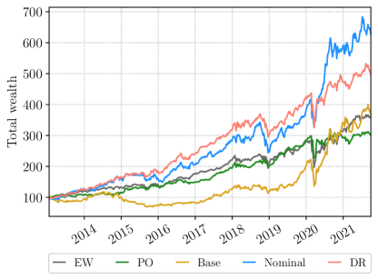
Figure 2: Experiment 1 – Wealth evolution

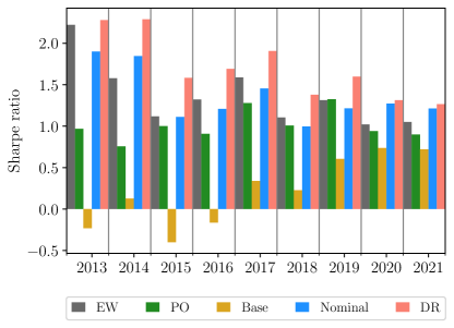
Figure 3: Experiment 1 – Cumulative Sharpe ratio. The cumulative Sharpe ratio is computed at year-end. Values are annualized.

Table 3: Experiment 1 – Results

	EW	PO	Base	Nom.	DR
Return (%)	15.6	13.4	16.1	23.4	20.1
Volatility (%)	14.9	15.3	25.0	18.8	15.5
Sharpe ratio	1.05	0.88	0.64	1.24	1.30
Note: Values are annualized.

3.2.2 Experiment 2: Learning $\delta$

The second experiment focused on understanding the improvement in performance by learning $\delta$; therefore, $\bm{\theta}$ and $\gamma$ were fixed. We focused on three investment systems: the predict-then-optimize (PO) system (since $\bm{\theta}$ and $\gamma$ are fixed, this is the same as the nominal system), the DR system with constant $\bm{\theta}$, $\gamma$ and $\delta$; and the DR system with constant $\bm{\theta}$ and $\gamma$, but with a learnable $\delta$. The difference in performance between the PO system and the DR system with all parameters fixed will highlight the benefit of adding some (not optimized) robustness, and the difference in performance between the DR systems with optimized $\delta$ and fixed $\delta$ is a measure of the impact of size of the uncertainty set. Details of the three systems are presented in Table 4. The out-of-sample financial performance of the three investment systems is summarized in Figure 4 and Table 5. The experimental results lead to the following observations.

• Impact of robustness without learning: The results for the PO system and the DR with no parameter learning show that, even when learning is not allowed, robustness has a positive impact on out-of-sample performance.

• Isolated learning of $\delta$: The results in Table 5 show that, although adding robustness improves the Sharpe ratio, solely optimizing $\delta$ can be detrimental to the system’s out-of-sample performance.

Table 4: Experiment 2 – List of models

	$\bm{\theta}$			$\gamma$			$\delta$
System	Val.	Lrn		Val.	Lrn		Val.	Lrn
PO	OLS	-		0.046	-		-	-
DR	OLS	✗		0.046	✗		0.312	✗
DR	OLS	✗		0.046	✗		0.312	✓
Note: Val, Initial value; Lrn, Learnable.

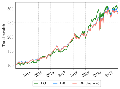
Figure 4: Experiment 2 – Wealth evolution

Table 5: Experiment 2 – Results

	PO	DR
		Const. $\delta$	Learn $\delta$
Return (%)	13.4	12.9	12.6
Volatility (%)	15.3	12.8	12.8
Sharpe ratio	0.88	1.01	0.99
Note: Values are annualized.

3.2.3 Experiment 3: Learning $\gamma$

The third experiment assessed the out-of-sample impact of learning $\gamma$. Therefore, here we experimented with only those systems involving $\gamma$, i.e. nominal system with constant $\bm{\theta}$, and a DR system with constant $\bm{\theta}$ and $\delta$ but with a learnable $\gamma$, with the PO system added as a baseline control. Details of the three systems are given in Table 6.

Table 6: Experiment 3 – List of models

	$\bm{\theta}$			$\gamma$			$\delta$
System	Val.	Lrn		Val.	Lrn		Val.	Lrn
PO	OLS	-		0.046	-		-	-
Nominal	OLS	✗		0.046	✓		-	-
DR	OLS	✗		0.046	✓		0.312	✗
Note(s): Val, Initial value; Lrn, Learnable.

The out-of-sample financial performance of the three investment systems is summarized in Figure 5 and Table 7. The experimental results lead to the following observations.

• Impact of robustness: The results of this experiment once again highlight the out-of-sample benefits of incorporating robustness into the system: the Sharpe ratio of the DR system is the highest. Although the PO system has the highest return, we must keep in mind that the task loss function was a weighted combination of Sharpe ratio and prediction error, meaning, by design, a higher Sharpe ratio is desirable.

• Isolated learning of $\gamma$: Comparing the PO system with the nominal system, we observe that only learning $\gamma$ may not be beneficial to the out-of-sample performance of a system. However, when robustness is incorporated into the system, the out-of-sample performance is greatly enhanced.

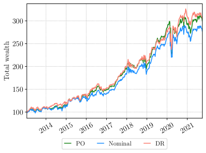
Figure 5: Experiment 3 – Wealth evolution

Table 7: Experiment 3 – Results

	PO	Nom.	DR
Return (%)	13.4	12.4	13.6
Volatility (%)	15.3	14.7	13.4
Sharpe ratio	0.88	0.84	1.02
Note(s): Values are annualized.

3.2.4 Experiment 4: Learning $\theta$

The fourth experiment assesses the out-of-sample impact of learning the prediction layer weights $\bm{\theta}$. We tested four investment systems: the PO system, the base system, the nominal system with constant $\gamma$, and the DR system with constant $\gamma$ and $\delta$. Details of the four systems are presented in Table 8.

Table 8: Experiment 4 – List of models

	$\bm{\theta}$			$\gamma$			$\delta$
System	Val.	Lrn		Val.	Lrn		Val.	Lrn
PO	OLS	-		0.046	-		-	-
Base	OLS	✓		-	-		-	-
Nominal	OLS	✓		0.046	✗		-	-
DR	OLS	✓		0.046	✗		0.312	✗
Note: Val, Initial value; Lrn, Learnable.

The out-of-sample financial performance of the four investment systems is presented in Figure 6 and Table 9. The experimental results lead to the following observations.

• Impact of incorporating a deviation risk measure: The difference in the out-of-sample performance between the base system and the PO system clearly highlights the benefit of the deviation risk measure – even though the base system learns $\bm{\theta}$, this is not enough to combat the inherent uncertainty of the portfolio returns.

• Learning $\bm{\theta}$: Learning $\theta$ becomes advantageous once a risk measure is added to the decision layer. The PO and nominal systems differ only in that the nominal system is able to learn values of $\bm{\theta}$ that differ from the OLS weights. Thus, as suggested by Donti et al., (2017), learning $\bm{\theta}$ enhances the mapping of the prediction layer from the feature space to the asset space to extract a higher quality decision, but only if the impact of prediction error in the decision layer is properly modeled.

• Impact of robustness: Comparing the nominal and DR systems, we can see that incorporating robustness may not always be advantageous, in particular when the robustness sizing parameter $\delta$ is not optimally calibrated. The results in Table 9 indicate that $\delta$ was set too conservative – even though the volatility of the DR system is lower than the nominal, it incurs a large opportunity cost with regards to the portfolio return.

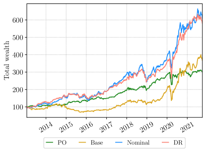
Figure 6: Experiment 4 – Wealth evolution

Table 9: Experiment 4 – Results

	PO	Base	Nom.	DR
Return (%)	13.4	16.1	23.0	22.3
Volatility (%)	15.3	25.0	19.1	18.5
Sharpe ratio	0.88	0.64	1.21	1.21
Note(s): Values are annualized.

Experiment with synthetic data

We simulate an investment universe with 10 assets and 5 features. The features were assumed to follow an uncorrelated zero-mean Brownian motion. The asset returns are generated from a linear model of the features,

$$\bm{y}_{t}=\bm{\alpha}+\bm{\beta}^{\top}\bm{x}_{t}+\bm{\xi}_{t}+\kappa_{t}\cdot\bm{\omega}_{t},$$

where $\bm{\alpha}\sim\mathcal{U}(0,0.015)\in\mathbb{R}^{n}$ is the vector of biases, $\bm{\beta}\in\mathbb{R}^{m\times n}$ where $\beta_{ij}\sim\mathcal{N}(0,0.015)\ \forall\ i,j$ is the matrix of weights (i.e., loadings), $\bm{\xi}_{t}\in\mathbb{R}^{n}$ where $\xi_{t}^{i}\sim\mathcal{N}(0,0.015)\ \forall\ i$ is a Gaussian noise vector, $\bm{\omega}_{t}\in\mathbb{R}^{n}$ where $\omega_{t}^{i}\sim\mathrm{Exp}(0.015)\ \forall\ i$ is an exponential noise vector, and $\kappa_{t}$ is a discrete random variable that takes the value $-1,0,1$ with probability 0.15, 0.7, 0.15, respectively, and serves to periodically perturb the asset return process bidirectionally with the magnitude of $\bm{\omega}_{t}$ in order to simulate ‘jumps’ in the asset returns.

The experimental data set is composed of 1,200 observations, with the first 840 reserved for training and the remaining 360 reserved for testing. However, unlike previous experiments, the synthetic data allows us to use a single fold for validation. Here, the complete training set is separated into a single training subset and single validation subset. The validation results are shown in Table 13 in Appendix F. The table also highlights the optimal hyperparameters selected for each system.

The fifth experiment explored the advantage of robustness when the prediction layer is more complex, e.g. a neural network with multiple hidden layers. Specifically, this experiment compares nominal and DR systems when the prediction layer is either a linear model, or neural network with two or three hidden layers. The neural networks had fully connected hidden layers, and the activation functions were rectified linear units (ReLUs).

The prediction layer in this experiment is initialized to random weights using the standard PyTorch (Paszke et al.,, 2019) initialization mechanism. This applies to all three prediction layer designs tested in this experiment. The initial values of the risk appetite parameter $\gamma$ and robustness parameter $\delta$ were sampled uniformly from the same intervals as the previous experiments (see Appendix E for the initialization methodology).

The objective of the experiment is to investigate whether robustness enhances the out-of-sample performance of a system with a more complex prediction layer, i.e., with a prediction layer that is more difficult to train accurately. To avoid biases pertaining to the design of the prediction layer, our assessment is based on a pairwise comparison between the two and three-layer systems. Details of the four investment systems are presented in Table 10.

Table 10: Experiment 5 – List of models

	$\bm{\theta}$			$\gamma$			$\delta$
System	Val.	Lrn		Val.	Lrn		Val.	Lrn
Linear
Nom.	Note 1	✓		0.089	✓		-	-
DR	Note 1	✓		0.089	✓		0.146	✓
2-layer
Nom.	Note 1	✓		0.081	✓		-	-
DR	Note 1	✓		0.081	✓		0.358	✓
3-layer
Nom.	Note 1	✓		0.072	✓		-	-
DR	Note 1	✓		0.072	✓		0.163	✓
Notes: (1) $\bm{\theta}$ is initialized to the same values for each pair of systems. (2) Val, Initial value; Lrn, Learnable.

The out-of-sample financial performance of the four investment systems is summarized in Figure 7 and Table 11. As previously noted, our assessment is based on a pairwise comparison between the linear, and two- and three-layer systems. The experimental results lead to the following observation.

• Impact of robustness: As indicated by the Sharpe ratios in Table 11, introducing distributional robustness greatly enhances the portfolio out-of-sample performance in all three cases. Recall that, unlike previous experiments where the prediction layers were initialized to the naturally intuitive OLS weights, the prediction layer in the current systems are initialized to fully randomized weights. Thus, through this experiment we can appreciate how robustness protects the portfolios from model error, particularly as the complexity of the prediction layer increases.

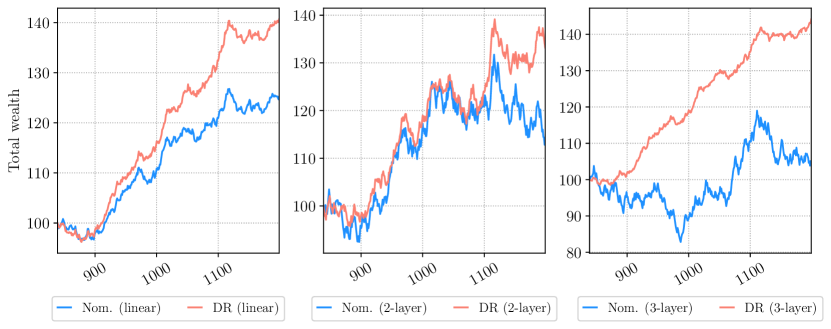
Figure 7: Experiment 5 – Wealth evolution

Table 11: Experiment 5 – Results

	Linear			2-layer			3-layer
	Nom.	DR		Nom.	DR		Nom.	DR
Return (%)	3.30	5.10		1.80	4.20		0.70	5.40
Vol. (%)	2.90	2.70		8.30	5.80		7.80	2.60
SR	1.16	1.88		0.21	0.73		0.08	2.11
Notes: (1) Vol, Volatility; SR, Sharpe ratio. (2) Values are annualized.

Conclusion

This paper introduces a novel DR end-to-end learning system for portfolio construction. Specifically, the system integrates a prediction layer of asset returns with a decision layer that selects portfolios by solving a DR optimization problem that explicitly incorporates model risk.

The decision layer in our end-to-end system consists of a DR portfolio selection problem that gets as input both the point prediction and the prediction errors. The prediction errors are used to define a deviation risk measure, and we penalize the performance of a portfolio with the worst-case risk over a set of probability measures. We show that, even though the deviation risk measure is not a linear function of the probability measure, one can still use convex duality to reformulate the minimax DR optimization problem into an equivalent minimization problem. This reformulation is critical to ensure that the gradients with respect to the task loss can be back-propagated to the prediction layer. Numerical experiments clearly show that incorporating model robustness via a DR layer leads to enhanced financial performance.

The parameters that control risk and robustness are learnable as part of the end-to-end system, meaning these two parameters are optimized directly from data based on the system’s out-of-sample performance. The learnability of the robustness parameter is a consequence of the convex duality that we use to reformulate the DR layer. Setting these two parameters in practice is a challenge, and our end-to-end system relieves the user from having to set them. Furthermore, our numerical experiments show that these parameters do significantly impact performance.

We have implemented our proposed robust end-to-end system in Python, and have made the code available on GitHub. We anticipate the DR approach to be very impactful for any application where model risk is an important consideration. Portfolio construction is only the beginning.

Appendix A Proof of Proposition 2.1

We begin with some preliminary information. Recall that $\bm{\epsilon}=\{\bm{\epsilon}_{j}\in\mathbb{R}^{n}:j=1,\ldots,T\}$ denotes the finite set of prediction error outcomes and $\bm{p}\in\mathcal{Q}$ is a PMF.

Here we prove the four properties of the deviation risk measure $f_{\bm{\epsilon}}$ outlined in Proposition 2.1.

1. $f_{\bm{\epsilon}}(\cdot,\bm{p}):\mathcal{Z}\rightarrow\mathbb{R}_{+}$ is convex for any fixed $\bm{p}\in\mathcal{Q}$.

   Proof.

   Since $R(X)$ is convex, it follows that

   $$h_{\bm{\epsilon}}(c,\bm{z},\bm{p})\triangleq\sum_{j=1}^{T}p_{j}\cdot R(\bm{\epsilon}_{j}^{\top}\bm{z}-c)$$ (8)

   is a convex function in $(c,\bm{z})$ for a fixed $\bm{p}$. Accordingly, $f_{\bm{\epsilon}}(\bm{z},\bm{p})=\min_{c}h_{\bm{\epsilon}}(c,\bm{z},\bm{p})$ is also a convex function of $\bm{z}$ for fixed $\bm{p}$ (Boyd and Vandenberghe,, 2004). ∎

2. $f_{\bm{\epsilon}}(\bm{z},\bm{p})\geq 0$ for all $\bm{p}\in\mathcal{Q}$ and $\bm{z}\in\mathcal{Z}$.

   Proof.

   By definition, we have that $R$ is a non-negative function. Moreover, $\bm{p}$ is constrained to the probability simplex (specifically, $p_{j}\geq 0\ \forall\ j$). Since, $f_{\bm{\epsilon}}$ is the sum of $T$ functions, each of which results from the product of two non-negative elements, then $f_{\bm{\epsilon}}(\bm{z},\bm{p})\geq 0$. ∎

3. $f_{\bm{\epsilon}}(\bm{z},\bm{p})$ is shift-invariant with respect to $\bm{\epsilon}$, i.e. $f_{\bm{\epsilon}+\bm{a}}(\bm{z},\bm{p})=f_{\bm{\epsilon}}(\bm{z},\bm{p})$ for any fixed vector $\bm{a}\in\mathbb{R}^{n}$.

   Proof.

   By definition, we have that

   $$f_{\bm{\epsilon}+\bm{a}}(\bm{z},\bm{p}) =\min_{c}\bigg{\{}\sum_{j=1}^{T}p_{j}\cdot R\big{(}(\bm{\epsilon}_{j}+\bm{a})^{\top}\bm{z}-c\big{)}\bigg{\}},$$

   $$=\min_{c}\bigg{\{}\sum_{j=1}^{T}p_{j}\cdot R\big{(}\bm{\epsilon}_{j}^{\top}\bm{z}-(c-\bm{a}^{\top}\bm{z})\big{)}\bigg{\}},$$

   $$=\min_{c^{\prime}}\bigg{\{}\sum_{j=1}^{T}p_{j}\cdot R\big{(}\bm{\epsilon}_{j}^{\top}\bm{z}-c^{\prime})\big{)}\bigg{\}},$$

   where $c^{\prime}=c-\bm{a}^{\top}\bm{z}$. The result follows from the last expression. ∎

4. $f_{\bm{\epsilon}}(\bm{z},\bm{p})$ is symmetric with respect to $\bm{\epsilon}$, i.e. $f_{\bm{\epsilon}}(\bm{z},\bm{p})=f_{-\bm{\epsilon}}(\bm{z},\bm{p})$.

   Proof.

   By definition, we have that

   $$f_{-\bm{\epsilon}}(\bm{z},\bm{p}) =\min_{c}\bigg{\{}\sum_{j=1}^{T}p_{j}\cdot R\big{(}-\bm{\epsilon}_{j}^{\top}\bm{z}-c\big{)}\bigg{\}},$$

   $$=\min_{c}\bigg{\{}\sum_{j=1}^{T}p_{j}\cdot R\big{(}\bm{\epsilon}_{j}^{\top}\bm{z}+c\big{)}\bigg{\}},$$ (9)

   $$=\min_{c^{\prime}}\bigg{\{}\sum_{j=1}^{T}p_{j}\cdot R\big{(}\bm{\epsilon}_{j}^{\top}\bm{z}-c^{\prime})\big{)}\bigg{\}},$$

   where $c^{\prime}=-c$, and (9) follows from the fact that $R(X)=R(-X)$. The result follows from the last expression. ∎

Appendix B Portfolio error variance

Recall that $\bm{\epsilon}=\{\bm{\epsilon}_{j}\in\mathbb{R}^{n}:j=1,\ldots,T\}$ denotes the finite set of prediction error outcomes. For a fixed distribution $\bm{p}\in\mathcal{Q}$, the expected error and its corresponding covariance matrix are

$$\bm{\mu}_{\bm{\epsilon}}(\bm{p}) \triangleq\sum_{j=1}^{T}p_{j}\cdot\bm{\epsilon}_{j},$$ (10)

$$\bm{\Sigma}_{\bm{\epsilon}}(\bm{p}) \triangleq\sum_{j=1}^{T}p_{j}\cdot\big{(}\bm{\epsilon}_{j}-\bm{\mu}_{\bm{\epsilon}}(\bm{p})\big{)}\big{(}\bm{\epsilon}_{j}-\bm{\mu}_{\bm{\epsilon}}(\bm{p})\big{)}^{\top},$$ (11)

where $\bm{\mu}_{\bm{\epsilon}}(\bm{p})\in\mathbb{R}^{n}$ and $\bm{\Sigma}_{\bm{\epsilon}}(\bm{p})\in\mathbb{R}^{n\times n}$. The matrix $\bm{\Sigma}_{\bm{\epsilon}}(\bm{p})$ results from the weighted sum of $T$ rank-1 symmetric matrices, meaning it is guaranteed to be positive semidefinite.

Note that $\bm{\Sigma}_{\bm{\epsilon}}(\bm{p})$ is a non-linear function of $\bm{p}$; consequently, the portfolio variance $\bm{z}^{\top}\hat{\bm{\Sigma}}_{\bm{\epsilon}}(\bm{p})\bm{z}$ is also non-linear in $\bm{p}$. Thus, in this form, the worst-case variance $\max_{\bm{p}\in\mathcal{P}(\delta)}\bm{z}^{\top}\hat{\bm{\Sigma}}_{\bm{\epsilon}}(\bm{p})\bm{z}$ does not have the correct convexity properties that allow one to reformulate the problem using duality. We resolve this issue by recasting the portfolio error variance into the form prescribed by Proposition 2.1, which yields the following corollary.

Corollary B.1.

For a fixed $\bm{z}\in\mathcal{Z}$ and $\bm{p}\in\mathcal{Q}$, the portfolio variance is

$$\bm{z}^{\top}\bm{\Sigma}_{\bm{\epsilon}}(\bm{p})\bm{z}=\min_{c}\ \sum_{j=1}^{T}p_{j}\cdot(\bm{\epsilon}_{j}^{\top}\bm{z}-c)^{2},$$

where $c\in\mathbb{R}$ is an unrestricted auxiliary variable.

Proof.

Let $h(c)=\sum_{j=1}^{T}p_{j}\cdot(\bm{\epsilon}_{j}^{\top}\bm{z}-c)^{2}$ and recall that $\sum_{j=1}^{T}p_{j}=1$. Then

$$\frac{dh}{dc} =2\sum_{j=1}^{T}(p_{j}\cdot c-p_{j}\cdot\bm{\epsilon}_{j}^{\top}\bm{z})$$

$$=2c-2\sum_{j=1}^{T}p_{j}\cdot\bm{\epsilon}_{j}^{\top}\bm{z},$$

$$\frac{d^{2}h}{dc^{2}} =2.$$

Since $d^{2}h/dc^{2}>0\ \forall c\in\mathbb{R}$, then $h(c)$ is strictly convex in $c$. Therefore, solving for $c$ such that $dh/dc=0$ suffices to find the unique global minimizer $c^{*}$,

$$\frac{dh}{dc}\bigg{|}_{c=c^{*}} =2c^{*}-2\sum_{j=1}^{T}p_{j}\cdot\bm{\epsilon}_{j}^{\top}\bm{z}=0,$$

$$c^{*} =\sum_{j=1}^{T}p_{j}\cdot\bm{\epsilon}_{j}^{\top}\bm{z},$$

for all $\bm{p}\in\mathcal{Q}$ and $\{\bm{\epsilon}_{j}:j=1,\ldots,T\}$. Then, by (10), we have

$$c^{*}=\sum_{j=1}^{T}p_{j}\cdot\bm{\epsilon}_{j}^{\top}\bm{z}=\bm{z}^{\top}\sum_{j=1}^{T}p_{j}\cdot\bm{\epsilon}_{j}=\bm{z}^{\top}\bm{\mu}_{\bm{\epsilon}}(\bm{p}).$$

Now, using (11), the portfolio error variance is

$$\bm{z}^{\top}\bm{\Sigma}_{\bm{\epsilon}}(\bm{p})\bm{z} =\sum_{j=1}^{T}p_{j}\cdot\bm{z}^{\top}\big{(}\bm{\epsilon}_{j}-\bm{\mu}_{\bm{\epsilon}}(\bm{p})\big{)}\big{(}\bm{\epsilon}_{j}-\bm{\mu}_{\bm{\epsilon}}(\bm{p})\big{)}^{\top}\bm{z}$$

$$=\sum_{j=1}^{T}p_{j}\cdot\Big{(}\bm{z}^{\top}\big{(}\bm{\epsilon}_{j}-\bm{\mu}_{\bm{\epsilon}}(\bm{p})\big{)}\Big{)}^{2}$$

$$=\sum_{j=1}^{T}p_{j}\cdot\big{(}\bm{z}^{\top}\bm{\epsilon}_{j}-\bm{z}^{\top}\bm{\mu}_{\bm{\epsilon}}(\bm{p})\big{)}^{2}$$

$$=\sum_{j=1}^{T}p_{j}\cdot(\bm{\epsilon}_{j}^{\top}\bm{z}-c^{*})^{2}$$

$$=\min_{c}\sum_{j=1}^{T}p_{j}\cdot(\bm{\epsilon}_{j}^{\top}\bm{z}-c)^{2},$$

as desired. ∎

Appendix C Dualizing the DR layer

Recall that $h_{\bm{\epsilon}}(c,\bm{z},\bm{p})$ in (8) is a convex function in $(c,\bm{z})$ for any fixed $\bm{p}\in\mathcal{Q}$. Moreover, $h_{\bm{\epsilon}}(c,\bm{z},\bm{p})$ is linear in $\bm{p}$ for any fixed $(c,\bm{z})\in\mathbb{R}\times\mathcal{Z}$. Thus, $h_{\bm{\epsilon}}(c,\bm{z},\bm{p})$ is convex–linear in $(c,\bm{z})$ and $\bm{p}$, respectively.

Fix $\bm{z}\in\mathcal{Z}$. Then, the minimax theorem for convex duality (Von Neumann,, 1928) implies that

$$\max_{\bm{p}\in\mathcal{P}(\delta)}f_{\bm{\epsilon}}(\bm{z},\bm{p}) =\max_{\bm{p}\in\mathcal{P}(\delta)}\min_{c\in\mathbb{R}}h_{\bm{\epsilon}}(c,\bm{z},\bm{p})$$

$$=\min_{c\in\mathbb{R}}\max_{\bm{p}\in\mathcal{P}(\delta)}\sum_{j=1}^{T}p_{j}\cdot R(\bm{\epsilon}_{j}^{\top}\bm{z}-c).$$

Next, we adapt the results in Ben-Tal et al., (2013) to write the maximization over $\bm{p}$ as a dual minimization problem. Note that this transformation is straightforward, and is only included for completeness.

Fix $(c,\bm{z})\in\mathbb{R}\times\mathcal{Z}$. From the definition of the ambiguity set $\mathcal{P}(\delta)$, it follows that the maximization problem in $\bm{p}$ is

$$\begin{array}[]{ll}\displaystyle\max_{\bm{p}}&\displaystyle\sum_{j=1}^{T}p_{j}\cdot R(\bm{\epsilon}_{j}^{\top}\bm{z}-c),\\ \ \text{s.t.}&\displaystyle\sum_{j=1}^{T}p_{j}=1,\\ &\displaystyle I_{\phi}(\bm{p},\bm{q})=\sum_{j=1}^{T}q_{j}\cdot\phi(p_{j}/q_{j})\leq\delta,\\ &\bm{p}\geq\bm{0}.\end{array}$$

Associate a dual variable $\xi$ with the constraint $\sum_{j=1}^{T}p_{j}=1$ and a dual variable $\lambda\geq 0$ with the constraint $I_{\phi}(\bm{p},\bm{q})\leq\delta$. Then, the Lagrangian dual function is

$$f_{\bm{\epsilon}}^{\delta}(\bm{z},c,\lambda,\xi)$$

$$\hskip 20.0pt\triangleq\max_{\bm{p}\geq\bm{0}}\sum_{j=1}^{T}p_{j}\cdot R(\bm{\epsilon}_{j}^{\top}\bm{z}-c)+\xi\cdot(1-\bm{1}^{\top}\bm{p})$$

$$\hskip 60.0pt+\lambda\cdot\bigg{(}\delta-\sum_{j=1}^{T}q_{j}\cdot\phi(p_{j}/q_{j})\bigg{)}$$

$$\hskip 20.0pt=\xi+\delta\cdot\lambda+\max_{\bm{p}\geq\bm{0}}\sum_{j=1}^{T}\Big{(}p_{j}\cdot\big{(}R(\bm{\epsilon}_{j}^{\top}\bm{z}-c)-\xi\big{)}$$

$$\hskip 135.0pt-\lambda\cdot q_{j}\cdot\phi(p_{j}/q_{j})\Big{)}$$

$$\hskip 20.0pt=\xi+\delta\cdot\lambda+\sum_{j=1}^{T}\max_{p_{j}\geq 0}\Big{(}p_{j}\cdot\big{(}R(\bm{\epsilon}_{j}^{\top}\bm{z}-c)-\xi\big{)}$$

$$\hskip 135.0pt-\lambda\cdot q_{j}\cdot\phi(p_{j}/q_{j})\Big{)}$$

$$\hskip 20.0pt=\xi+\delta\cdot\lambda+\sum_{j=1}^{T}q_{j}\cdot\max_{s\geq 0}\Big{(}s\cdot\big{(}R(\bm{\epsilon}_{j}^{\top}\bm{z}-c)-\xi\big{)}$$

$$\hskip 178.0pt-\lambda\cdot\phi(s)\Big{)}$$

$$\hskip 20.0pt=\xi+\delta\cdot\lambda+\sum_{j=1}^{T}q_{j}\cdot(\lambda\phi)^{*}\big{(}R(\bm{\epsilon}_{j}^{\top}\bm{z}-c)-\xi\big{)}$$

$$\hskip 20.0pt=\xi+\delta\cdot\lambda+\frac{\lambda}{T}\sum_{j=1}^{T}\phi^{*}\bigg{(}\frac{R(\bm{\epsilon}_{j}^{\top}\bm{z}-c)-\xi}{\lambda}\bigg{)}.$$ (12)

Note that we arrive at (12) by taking the convex conjugate of $\phi$ and by using the identity $(\lambda\phi)^{*}(w)=\lambda\cdot\phi^{*}(w/\lambda)$ for $\lambda\geq 0$. Additionally, recall that our nominal assumption states that $q_{j}=1/T\ \forall j$.

Since the conjugate $\phi^{*}$ of a $\phi$-divergence is a convex function, it follows that the Lagrangian function $f_{\bm{\epsilon}}^{\delta}(\bm{z},c,\lambda,\xi)$ is jointly convex in $(\bm{z},c,\lambda,\xi)\in\mathcal{Z}\times\mathbb{R}\times\mathbb{R}_{+}\times\mathbb{R}$ (see Ben-Tal et al., (2013) for details).

Finally, note that the Lagrangian dual in (12) above is the same as the distributionally robust deviation risk measure in (5). The above steps demonstrate the equivalence between the minimax problem in (3) and the minimization problem in (4), i.e.,

$$\min_{\bm{z}\in\mathcal{Z},c}\ \max_{\bm{p}\in\mathcal{P}(\delta)}\sum_{j=1}^{T}p_{j}\cdot R(\bm{\epsilon}_{j}^{\top}\bm{z}-c)-\gamma\cdot\hat{\bm{y}}_{t}^{\top}\bm{z}$$

$$\hskip 35.0pt\iff\min_{\bm{z}\in\mathcal{Z},\ \lambda\geq 0,\ \xi,\ c}\ f_{\bm{\epsilon}}^{\delta}(\bm{z},c,\lambda,\xi)-\gamma\cdot\hat{\bm{y}}_{t}^{\top}\bm{z}.$$

Appendix D Tractable reformulations

Recall that the DR layer in (4) corresponds to the following minimization problem,

$$\begin{aligned} &\min_{\bm{z},\lambda,\xi,c}\xi+\delta\cdot\lambda+\frac{\lambda}{T}\sum_{j=1}^{T}\phi^{*}\bigg{(}\frac{R(\bm{\epsilon}_{j}^{\top}\bm{z}-c)-\xi}{\lambda}\bigg{)}-\gamma\cdot\hat{\bm{y}}_{t}^{\top}\bm{z}\end{aligned}$$

$$\begin{aligned} &\ \text{s.t.}&\lambda&\geq 0\\ &&\bm{z}&\in\mathcal{Z}\end{aligned}$$

The computational tractability of this optimization problem depends on the complexity of the $\phi$-divergence selected to construct the ambiguity set $\mathcal{P}(\delta)$.

Hellinger distance

The Hellinger distance is defined as

$$I_{\phi}^{H}(\bm{p},\bm{q})\triangleq\sum_{j=1}^{T}q_{j}\cdot\phi_{H}(p_{j}/q_{j})=\sum_{j=1}^{T}\big{(}\sqrt{p_{j}}-\sqrt{q_{j}}\big{)}^{2}$$

where $\phi_{H}(w)\triangleq(\sqrt{w}-1)^{2}$ for $w\geq 0$. The convex conjugate

$$\phi_{H}^{*}(s)\triangleq\frac{s}{1-s}\ \text{ for }s<1.$$

If we construct the probability ambiguity set $\mathcal{P}(\delta)$ using the Hellinger distance, then the DR layer becomes a highly non-linear convex optimization problem. Nevertheless, the problem can be reformulated into a tractable problem as follows. Let $h(s)\triangleq 1/(1-s)=\phi_{H}^{*}(s)+1$. Then $h^{-1}(s)=1-1/s$ and the objective function is

$$\xi+(\delta-1)\cdot\lambda+\frac{1}{T}\sum_{j=1}^{T}\lambda\cdot h\bigg{(}\frac{R(\bm{\epsilon}_{j}^{\top}\bm{z}-c)-\xi}{\lambda}\bigg{)}-\gamma\cdot\hat{\bm{y}}_{t}^{\top}\bm{z}.$$

Next, introduce the auxiliary variable $\bm{\beta}\in\mathbb{R}^{T}$ and let

$$\beta_{j}\geq\lambda\cdot h\bigg{(}\frac{R(\bm{\epsilon}_{j}^{\top}\bm{z}-c)-\xi}{\lambda}\bigg{)}$$

$$\hskip 35.0pt\iff h^{-1}\bigg{(}\frac{\beta_{j}}{\lambda}\bigg{)}\geq\frac{R(\bm{\epsilon}_{j}^{\top}\bm{z}-c)-\xi}{\lambda}$$

$$\hskip 35.0pt\iff\hskip 11.0pt\lambda-\frac{\lambda^{2}}{\beta_{j}}\geq R(\bm{\epsilon}_{j}^{\top}\bm{z}-c)-\xi.$$

Note that, since $\phi_{H}^{*}(s)$ requires that $s<1$, then $\bm{\beta}\geq\bm{0}$.

Finally, introduce the auxiliary variable $\bm{\tau}\in\mathbb{R}_{+}^{T}$ to arrive at the tractable reformulation of the Hellinger-based DR layer,

$$\begin{aligned} &\min_{\bm{z},\lambda,\xi,c,\bm{\beta},\bm{\tau}}\xi+(\delta-1)\cdot\lambda+\frac{1}{T}\sum_{j=1}^{T}\beta_{j}-\gamma\cdot\hat{\bm{y}}_{t}^{\top}\bm{z}\end{aligned}$$

$$\begin{aligned} &\quad\ \ \text{s.t.}&\xi+\lambda&\geq R(\bm{\epsilon}_{j}^{\top}\bm{z}-c)+\tau_{j},&j=1,\dots,T\\ &&\beta_{j}\tau_{j}&\geq\lambda^{2},&j=1,\dots,T\\ &&\bm{\beta},\bm{\tau}&\geq\bm{0},\\ &&\lambda&\geq 0,\\ &&\bm{z}&\in\mathcal{Z}.\end{aligned}$$

Note that the hyperbolic constraint, $\beta_{j}\tau_{j}\geq\lambda^{2}$, can be equivalently written as a rotated second-order cone constraint.

Variation distance

The Variation distance is defined as

$$I_{\phi}^{V}(\bm{p},\bm{q})\triangleq\sum_{j=1}^{T}q_{j}\cdot\phi_{V}(p_{j}/q_{j})=\sum_{j=1}^{T}\big{|}p_{j}-q_{j}\big{|}$$

where $\phi_{V}(w)\triangleq|w-1|$ for $w\geq 0$. The conjugate

$$\phi_{V}^{*}(s)\triangleq\begin{cases}-1,&s\leq-1\\ s,&-1\leq s\leq 1\end{cases}.$$

The tractable reformulation presented here is adapted from Ben-Tal et al., (2013). Introduce the auxiliary variable $\bm{\beta}\in\mathbb{R}^{T}$. Then,

$$\begin{aligned} &\min_{\bm{z},\lambda,\xi,c,\bm{\beta}}\xi+\delta\cdot\lambda+\frac{1}{T}\sum_{j=1}^{T}\beta_{j}-\gamma\cdot\hat{\bm{y}}_{t}^{\top}\bm{z}\end{aligned}$$

$$\begin{aligned} &\ \text{s.t.}&\beta_{j}&\geq-\lambda,&j=1,\dots,T\\ &&\beta_{j}&\geq R(\bm{\epsilon}_{j}^{\top}\bm{z}-c)-\xi,&j=1,\dots,T\\ &&\lambda&\geq R(\bm{\epsilon}_{j}^{\top}\bm{z}-c)-\xi,&j=1,\dots,T\\ &&\lambda&\geq 0,\\ &&\bm{z}&\in\mathcal{Z}.\end{aligned}$$

Appendix E Initializing $\gamma$ and $\delta$ during experiments

The initial value for the parameter $\gamma$ was randomly sampled from a uniform distribution over a finite interval. The upper and lower boundaries of this interval are set such that the nominal value of the deviation risk measure, i.e. portfolio error variance, and the nominal return are comparable for the equal weight portfolio, i.e. $\hat{z}_{i}=1/n$ for $i=1,\ldots,n$. Note that the error variance was computed using errors corresponding to a linear prediction model with OLS weights.

Using the same training set as Section 3 with a sample set of $T=104$ prediction errors, we obtained samples of plausible $\gamma$ values as follows,

$$\hat{\gamma}_{j}=\frac{\hat{\bm{z}}^{\top}\bm{\Sigma}_{\bm{\epsilon}}(\bm{q})\hat{\bm{z}}}{|\hat{\bm{y}}_{j}^{\top}\hat{\bm{z}}|}\quad\text{for}\ j=T+1,\ldots,T_{0},$$

where $\bm{\Sigma}_{\bm{\epsilon}}(\bm{q})$ is calculated as in (11). To ensure reasonable emphasis is given to the deviation risk measure, we set the lower and upper bounds for the interval for $\gamma$ to the 1st and 25th percentiles of the sample set, respectively. This gave us the interval $[0.02,0.10]$.

The initial value for $\delta$ was also sampled from a uniform distribution over a finite interval. For the Hellinger distance, which we use for our experiments, the maximum distance is $\delta_{\max}=\max_{p}I^{H}_{\phi}(p,q)=2(1-1/\sqrt{T})$, where the nominal distribution $\bm{q}=\frac{1}{T}$. The theoretical upper bound is a useful benchmark, but we note that this is an extreme and implausible value. Thus, we set the upper bound $\delta_{\text{up}}=0.25\cdot\delta_{\text{max}}$, while we set the lower bound $\delta_{\text{lo}}=0.05\cdot\delta_{\text{max}}$. In Experiments 1–4, where $T=104$, the sampling interval is $\delta\in[0.09,0.45]$. Initializing $\delta$ from this interval ensures that the distance between $\bm{p}$ and $\bm{q}$ is not too extreme at the start of the training process.

Appendix F Validation and hyperparameter selection

Table 12: Average validation loss in Experiments 1–4

$\eta$	Epochs	Base	Nominal				DR
			Learned parameters				Learned parameters
			$\bm{\theta},\gamma$	$\gamma$	$\bm{\theta}$		$\bm{\theta},\gamma,\delta$	$\delta$	$\gamma$	$\gamma,\delta$	$\bm{\theta}$
0.0050	30	-0.1522	-0.1769	-0.1682	-0.1747		-0.1708	-0.1897	-0.1841	-0.1817	-0.1714
0.0125	30	-0.1130	-0.1784	-0.1672	-0.1854		-0.1723	-0.1779	-0.1775	-0.1766	-0.1698
0.0200	30	-0.1097	-0.1809	-0.1675	-0.1874		-0.1412	-0.1785	-0.1749	-0.1766	-0.1603
0.0050	40	-0.1372	-0.1793	-0.1680	-0.1733		-0.1705	-0.1888	-0.1817	-0.1787	-0.1734
0.0125	40	-0.1109	-0.1767	-0.1675	-0.1828		-0.1703	-0.1782	-0.1762	-0.1770	-0.1746
0.0200	40	-0.1044	-0.1819	-0.1675	-0.1848		-0.1365	-0.1779	-0.1752	-0.1756	-0.1609
0.0050	50	-0.1278	-0.1820	-0.1679	-0.1727		-0.1748	-0.1868	-0.1807	-0.1780	-0.1719
0.0125	50	-0.1091	-0.1772	-0.1674	-0.1839		-0.1752	-0.1780	-0.1757	-0.1757	-0.1718
0.0200	50	-0.1079	-0.1887	-0.1683	-0.1854		-0.1329	-0.1780	-0.1755	-0.1679	-0.1649
0.0050	60	-0.1267	-0.1853	-0.1679	-0.1754		-0.1805	-0.1777	-0.1798	-0.1779	-0.1689
0.0125	60	-0.1094	-0.1807	-0.1677	-0.1846		-0.1826	-0.1779	-0.1761	-0.1680	-0.1653
0.0200	60	-0.0978	-0.1950	-0.1684	-0.1838		-0.1630	-0.1781	-0.1760	-0.1674	-0.1756
0.0050	80	-0.1069	-0.1888	-0.1679	-0.1792		-0.1779	-0.1779	-0.1788	-0.1765	-0.1692
0.0125	80	-0.1036	-0.1804	-0.1682	-0.1846		-0.1695	-0.1779	-0.1762	-0.1675	-0.1662
0.0200	80	-0.0858	-0.1907	-0.1679	-0.1703		-0.1604	-0.1781	-0.1773	-0.1673	-0.1731
0.0050	100	-0.1032	-0.1914	-0.1679	-0.1815		-0.1757	-0.1779	-0.1780	-0.1676	-0.1690
0.0125	100	-0.1045	-0.1740	-0.1679	-0.1791		-0.1582	-0.1779	-0.1765	-0.1676	-0.1662
0.0200	100	-0.0932	-0.1909	-0.1680	-0.1523		-0.1601	-0.1781	-0.1773	-0.1673	-0.1592
Notes: (1) Average validation loss of end-to-end systems over four training folds. (2) The lowest validation score of each system is bolded.

Table 13: Validation loss in Experiment 5

$\eta$	Epochs	Linear			2-layer			3-layer
		Nom.	DR		Nom.	DR		Nom.	DR
0.0050	20	-0.2255	-0.1167		-0.1376	0.0350		-0.0603	-0.1373
0.0125	20	-0.2391	-0.0725		-0.1966	-0.0433		-0.0601	-0.1968
0.0200	20	-0.2677	-0.2475		-0.3014	-0.2481		-0.0408	-0.2576
0.0050	40	-0.2483	-0.2237		-0.1377	0.0348		-0.0603	-0.0645
0.0125	40	-0.2740	-0.2270		-0.1965	-0.2419		-0.0601	-0.1758
0.0200	40	-0.2564	-0.2140		-0.2481	-0.2116		-0.0404	-0.0423
0.0050	60	-0.2796	-0.2346		-0.1377	-0.1143		-0.0603	-0.1177
0.0125	60	-0.2135	-0.1729		-0.1965	-0.2088		-0.0602	-0.0832
0.0200	60	-0.2628	-0.1796		-0.2545	-0.2115		-0.0405	-0.1353
Notes: (1) Validation loss of end-to-end systems over a single training fold. (2) The lowest validation score of each system is bolded.

References

- Agrawal et al., (2019) Agrawal, A., Amos, B., Barratt, S., Boyd, S., Diamond, S., and Kolter, J. Z. (2019). Differentiable convex optimization layers. Advances in Neural Information Processing Systems, 32:9562–9574.
- Amos, (2019) Amos, B. (2019). Differentiable optimization-based modeling for machine learning. PhD thesis, PhD thesis. Carnegie Mellon University.
- Amos and Kolter, (2017) Amos, B. and Kolter, J. Z. (2017). Optnet: Differentiable optimization as a layer in neural networks. In International Conference on Machine Learning, pages 136–145. PMLR.
- Amos et al., (2018) Amos, B., Rodriguez, I. D. J., Sacks, J., Boots, B., and Kolter, J. Z. (2018). Differentiable mpc for end-to-end planning and control. In Proceedings of the 32nd International Conference on Neural Information Processing Systems, pages 8299–8310.
- Ben-Tal et al., (2013) Ben-Tal, A., Den Hertog, D., De Waegenaere, A., Melenberg, B., and Rennen, G. (2013). Robust solutions of optimization problems affected by uncertain probabilities. Management Science, 59(2):341–357.
- Bengio, (1997) Bengio, Y. (1997). Using a financial training criterion rather than a prediction criterion. International Journal of Neural Systems, 8(04):433–443.
- Bertsimas et al., (2018) Bertsimas, D., Gupta, V., and Kallus, N. (2018). Data-driven robust optimization. Mathematical Programming, 167(2):235–292.
- Best and Grauer, (1991) Best, M. J. and Grauer, R. R. (1991). On the sensitivity of mean-variance-efficient portfolios to changes in asset means: some analytical and computational results. The review of financial studies, 4(2):315–342.
- Boyd and Vandenberghe, (2004) Boyd, S. and Vandenberghe, L. (2004). Convex optimization. Cambridge university press.
- Broadie, (1993) Broadie, M. (1993). Computing efficient frontiers using estimated parameters. Annals of Operations Research, 45(1):21–58.
- Butler and Kwon, (2021) Butler, A. and Kwon, R. H. (2021). Integrating prediction in mean-variance portfolio optimization.
- Calafiore, (2007) Calafiore, G. C. (2007). Ambiguous risk measures and optimal robust portfolios. SIAM Journal on Optimization, 18(3):853–877.
- Chopra and Ziemba, (1993) Chopra, V. K. and Ziemba, W. T. (1993). The effect of errors in means, variances, and covariances on optimal portfolio choice. Journal of Portfolio Management, pages 6–11.
- Costa and Kwon, (2020) Costa, G. and Kwon, R. H. (2020). A robust framework for risk parity portfolios. Journal of Asset Management, 21:447–466.
- Costa and Kwon, (2021) Costa, G. and Kwon, R. H. (2021). Data-driven distributionally robust risk parity portfolio optimization. arXiv preprint arXiv:2110.06464.
- Delage and Ye, (2010) Delage, E. and Ye, Y. (2010). Distributionally robust optimization under moment uncertainty with application to data-driven problems. Operations Research, 58(3):595–612.
- DeMiguel et al., (2009) DeMiguel, V., Garlappi, L., and Uppal, R. (2009). Optimal versus naive diversification: How inefficient is the 1/n portfolio strategy? The review of Financial studies, 22(5):1915–1953.
- Domahidi et al., (2013) Domahidi, A., Chu, E., and Boyd, S. (2013). ECOS: An SOCP solver for embedded systems. In European Control Conference (ECC), pages 3071–3076.
- Donti et al., (2017) Donti, P. L., Amos, B., and Kolter, J. Z. (2017). Task-based end-to-end model learning in stochastic optimization. In Proceedings of the 31st International Conference on Neural Information Processing Systems, pages 5490–5500.
- Elmachtoub et al., (2020) Elmachtoub, A., Liang, J. C. N., and McNellis, R. (2020). Decision trees for decision-making under the predict-then-optimize framework. In International Conference on Machine Learning, pages 2858–2867. PMLR.
- Elmachtoub and Grigas, (2021) Elmachtoub, A. N. and Grigas, P. (2021). Smart “predict, then optimize”. Management Science.
- Fabozzi et al., (2007) Fabozzi, F. J., Kolm, P. N., Pachamanova, D. A., and Focardi, S. M. (2007). Robust portfolio optimization. Journal of Portfolio Management, 33(3):40.
- French, (2021) French, K. R. (2021). Data library. [Online; accessed 10-Dec-2021].
- Goldfarb and Iyengar, (2003) Goldfarb, D. and Iyengar, G. (2003). Robust portfolio selection problems. Mathematics of Operations Research, 28(1):1–38.
- Kannan et al., (2020) Kannan, R., Bayraksan, G., and Luedtke, J. R. (2020). Residuals-based distributionally robust optimization with covariate information. arXiv preprint arXiv:2012.01088.
- Kingma and Ba, (2014) Kingma, D. P. and Ba, J. (2014). Adam: A method for stochastic optimization. arXiv preprint arXiv:1412.6980.
- LeCun et al., (2005) LeCun, Y., Muller, U., Ben, J., Cosatto, E., and Flepp, B. (2005). Off-road obstacle avoidance through end-to-end learning. In Proceedings of the 18th International Conference on Neural Information Processing Systems, pages 739–746.
- Merton, (1980) Merton, R. C. (1980). On estimating the expected return on the market: An exploratory investigation. Journal of financial economics, 8(4):323–361.
- Paszke et al., (2019) Paszke, A., Gross, S., Massa, F., Lerer, A., Bradbury, J., Chanan, G., Killeen, T., Lin, Z., Gimelshein, N., Antiga, L., Desmaison, A., Kopf, A., Yang, E., DeVito, Z., Raison, M., Tejani, A., Chilamkurthy, S., Steiner, B., Fang, L., Bai, J., and Chintala, S. (2019). Pytorch: An imperative style, high-performance deep learning library. In Wallach, H., Larochelle, H., Beygelzimer, A., d’Alché Buc, F., Fox, E., and Garnett, R., editors, Advances in Neural Information Processing Systems 32, pages 8024–8035. Curran Associates, Inc.
- Rockafellar et al., (2006) Rockafellar, R. T., Uryasev, S., and Zabarankin, M. (2006). Generalized deviations in risk analysis. Finance and Stochastics, 10(1):51–74.
- Scarf, (1958) Scarf, H. (1958). A min-max solution of an inventory problem. Studies in the mathematical theory of inventory and production, pages 201–209.
- Sharpe, (1994) Sharpe, W. F. (1994). The sharpe ratio. Journal of Portfolio Management, 21(1):49–58.
- Thomas et al., (2006) Thomas, R. W., Friend, D. H., DaSilva, L. A., and MacKenzie, A. B. (2006). Cognitive networks: adaptation and learning to achieve end-to-end performance objectives. IEEE Communications magazine, 44(12):51–57.
- Tütüncü and Koenig, (2004) Tütüncü, R. H. and Koenig, M. (2004). Robust asset allocation. Annals of Operations Research, 132(1-4):157–187.
- Uysal et al., (2021) Uysal, A. S., Li, X., and Mulvey, J. M. (2021). End-to-end risk budgeting portfolio optimization with neural networks.
- Von Neumann, (1928) Von Neumann, J. (1928). Zur theorie der gesellschaftsspiele. Mathematische annalen, 100(1):295–320.
- Zhang et al., (2021) Zhang, C., Zhang, Z., Cucuringu, M., and Zohren, S. (2021). A universal end-to-end approach to portfolio optimization via deep learning. arXiv preprint arXiv:2111.09170.
- Zhang et al., (2020) Zhang, Z., Zohren, S., and Roberts, S. (2020). Deep learning for portfolio optimization. The Journal of Financial Data Science, 2(4):8–20.