Black holes in dRGT massive gravity with the signature of EHT observations of M87*

Abstract

The recent Event Horizon Telescope (EHT) observations of the M87* have led to a surge of interest in studying the shadow of black holes. Besides, investigation of time evolution and lifetime of black holes helps us to veto/restrict some theoretical models in gravitating systems. Motivated by such exciting properties, we study optical features of black holes, such as the shadow geometrical shape and the energy emission rate in modified gravity. We consider a charged AdS black hole in dRGT massive gravity and look for criteria to restrict the free parameters of the theory. The main goal of this paper is to compare the shadow of the mentioned black hole in a rotating case with the EHT data to obtain the allowed regions of the model parameters. Therefore, we employ the Newman-Janis algorithm to build the rotating counterpart of static solution in dRGT massive gravity. We also calculate the energy emission rate for the rotating case and discuss how the rotation factor and other parameters affect the emission of particles around the black holes.

I Introduction

The existence of a mysterious object known as a black hole (BH) is one of the important predictions of General Relativity (GR). In this regard, it has been proved that a BH really can form using ingenious mathematical methods by Penrose in 1965 Penrose . One of the interesting records of the existence of a BH is related to the gravitational wave, which was detected by the advanced LIGO/Virgo collaboration in 2016 LVCI . This record provides a constraint on the modified theories of gravity, for example, the existence of a tight bound on the graviton mass LVCII , or the speed of gravitational wave Cornish . Another strong record is related to the first image of a BH, which was detected by the Event Horizon Telescope in 2019 Akiyama . It may impose some constraint on properties of BHs constrainETHI ; constrainETHII ; constrainETHIII ; constrainETHIV ; constrainETHV , and parameters of modified theories of gravity ModM87I ; ModM87II . These reasons motivate us to study theoretical BHs in the light of observational data, which are receiving much attention today.

Some interesting modified theories of gravity have been proposed since our Universe expands with an acceleration AccUniI ; AccUniII , whereas GR cannot describe it, properly. Massive gravity is one of the extraordinary theories of gravity, which modifies gravitational effects by weakening it at a large scale compared to GR. On the other hand, to satisfy the concrete observations, it reduces to GR at small scales. The nonzero mass of gravitons in massive gravity has an upper limit obtained by recent observations of the advanced LIGO/Virgo collaboration LVCII . In addition, it was indicated that the mass of graviton might be variable. Indeed, the mass of gravity is tiny in the usual weak gravity environments. In contrast, it becomes much more significant in the strong gravity regime such as compact objects and BHs Variablegraviton . Appropriate description of rotation curves of the Milky Way and spiral galaxies Panpanich ; the existence of massive neutron stars neutronS and super-Chandrasekhar white dwarfs whitedwarf ; explaining the current observations related to dark matter darkMI ; darkMII ; the existence of a remnant for BH remnantI ; remnantII , are some interesting achievements in the context of massive gravity.

In 1939, Fierz and Pauli introduced a class of massive gravity theory in the flat background, in which the interaction terms added to GR FPmassive . This theory of massive gravity suffers from a discontinuity, which is known as van Dam-Veltman-Zakharov (vDVZ) discontinuity vDVZI ; vDVZII . In order to remove this discontinuity, nonlinear-massive gravity was introduced by Vainshtein Vainshtein . Afterward, Boulware and Deser have shown that such nonlinear generalizations generate a ghost instability, which is known as Boulware-Deser (BD) ghost BDghost . Arkani-Hamed et al. have resolved these problems by introducing Stückelberg fields, which lead to a class of potential energies depending on the gravitational metric and an internal Minkowski metric (reference metric) Arkani-Hamed . Finally, a new version of massive gravity was introduced by de Rham, Gabadadze, and Tolley (dRGT) dRGTI ; dRGTII , which is free of vDVZ discontinuity and BD ghost in arbitrary dimensions HassanI . This theory of massive gravity is known as dGRT massive gravity. Notably, there are two metric tensors in dRGT massive gravity, one of which is a fixed spacetime background. The generalization of fixed metric to dynamical metric was expanded by Hassan and Rosen, later known as the bimetric or bi-gravity theory bimetric . However, we consider the original massive gravity with a fixed background (dRGT massive gravity) in this work.

The establishment of a firm theoretical foundation of dRGT massive gravity has opened the possibility of studying its astrophysical and cosmological applications. In this regard, BH solutions with interesting properties have been obtained by considering the massive gravity in Refs. BHmassI ; BHmassVI ; BHmassIX ; BHmassXII ; BHmassXIV . In the astrophysics context, the properties of compact objects such as relativistic stars massstarI ; massstarII , neutron stars neutronS ; neutronSI , and white dwarfs whitedwarf , in this massive gravity have been evaluated. Considering dRGT massive gravity, the effect of helicity-0 mode, which remains elusive after analysis of cosmological perturbation around an open Friedmann–Lemaitre–Robertson–Walker universe, was evaluated in Ref. Chiang . In addition, the cosmological behavior Leon , bounce and cyclic cosmology Cai , graviton mass as a candidate for dark matter Aoki , and other studies have been done for finding some constraints on parameters of massive gravity by considering observational cosmological data consII ; consVI .

Recently, research in astrophysical BHs has gained much attention due to the breakthrough discovery of the reconstruction of the event-horizon-scale images of the supermassive BH in the galaxy M87* by the EHT project Akiyama ; Akiyama2019b . It was the first direct evidence of the existence of BHs compatible with the prediction of GR. Although the first image of the BH does not allow one to identify the BH geometry clearly, the principal strategy for improving measurements should lead to much higher resolution in the future Goddi2016 . So, one cannot underestimate theoretical efforts to calculate forms of shadows cast by BHs in various theories of gravity and astrophysical environments. The BH shadow is the optical appearance feature of the BH when a bright distant source is behind it. It appears as a two-dimensional dark zone for a distant observer, like us on Earth. The shadow of a BH can provide us with information about the BH and serve as a useful tool for testing GR. For a non-rotating BH, the boundary of the shadow is a perfect circle and was first studied by Synge Synge1966 and later by Luminet, who further considered the effect of a thin accretion disk on the shadow Luminet1979 . While the rotating case has an elongated shape in the direction of the rotation axis due to the dragging effect Bardeen1973 . The BH shadow has become a hot topic among researchers for the simple fact to evaluate the soon-expected observational data best. Shadows in various BH spacetimes have been studied extensively in the literature in the last decades Tsukamoto2018 ; Wei2013 ; Bambi2010 . This topic has also been extended to BHs in modified GR Amarilla2010 ; Kumar2021 , to BHs with higher or extra dimensions Papnoi2014 ; Pratap2017 , and BHs surrounded by plasma Atamurotov2015 . After the EHT announcement, a large amount of research has been devoted to calculating the shadows of a vast class of BH solutions and the confrontation with the extracted information from the EHT BH shadow image of M87* Davoudiasl2019 ; Konoplya2019 .

Although, in preliminary studies in the context of black hole shadow, the BH was assumed to be eternal, i.e., spacetime was assumed to be time-independent, recent astronomical observations have indicated that our Universe is currently undergoing a phase of accelerated expansion. This reveals the fact that the BH shadow can be dependent on time. Although the effect of the cosmological expansion is negligible for the BH candidates at the center of the Milky Way galaxy and at the centers of nearby galaxies, its influence on the shadow size will be significant for galaxies at a larger distance Perlick2018 . In the context of standard cosmology, based on GR, this acceleration cannot be explained unless by introducing an unknown energy component so-called dark energy. Another way to explain such acceleration is the modification of GR. One of the well-known candidates for dark energy scenarios is the cosmological constant. Recently, the role of the cosmological constant in gravitational lensing has been extensively studied Piattella2016 ; Butcher2016 ; Faraoni2017 ; Zhang2017bc ; Zhao2015ab . As we know, the shadow and photon ring are caused by the light deflection or gravitational lensing by BHs. So, one can inspect the effect of the cosmological constant on the shadow of black holes Haroon2019 ; Firouzjaee2019 . It is worth noting that although the expansion of the Universe was based on a positive cosmological constant, there is some evidence showing that it can be associated with a negative cosmological constant. The first one is through observational Hubble constant data. As we know, an interesting method for investigating the accelerated cosmic expansion and studying dark energy properties is through the Hubble constant, measured as a function of cosmological redshift Zhang2007fd ; Wan2007mn ; Ma2011kj . Investigating the behavior of $H(z)$ in low redshift data showed that the dark energy density has a negative minimum for certain redshift ranges, which can be simply modeled via a negative cosmological constant Dutta2020 . The second reason is through supernova data. Although according to the high-redshift supernova, the expansion of the Universe is accelerating due to a positive cosmological constant, it should be noted that the supernova data themselves derive a negative mass density in the Universe AccUniI ; AccUniII which can be equivalent to a negative cosmological constant Farnes2018 . Several galaxy cluster observations have inferred the presence of a negative mass in cluster environments. According to Ref. Farnes2018 , the introduction of negative masses can lead to an AdS space. Another reason to consider a negative cosmological constant is the concept of stability of the accelerating Universe. The possibility of de Sitter expanding spacetime with a constant internal space was investigated in Ref. Maeda2014a and was shown that the de Sitter solution would be stable just in the presence of the negative cosmological constant.

The manuscript is structured as follows: In Sec. II, we briefly review the charged AdS BH solution in dRGT massive gravity. In Subsec. II.1, we determine the null geodesics equations as well as the radius of the photon sphere and shadow, and we investigate the ratio of shadow radius and photon sphere to find an acceptable optical behavior. In Subsec. II.2, we calculate the energy emission rate and explore the effect of different parameters on the emission of particles around the BH. In Sec. III, by applying the Newman-Janis algorithm, we obtain the rotating charged AdS BH solution in dRGT massive gravity. The shadow geometrical shape and the energy emission rate for this type of solution are investigated in Subsec. III.1 and Subsec. III.2, respectively. In Sec. IV, we confront the obtained shadow of the rotating charged case with the EHT image of the supermassive object in M87*, and we extract explicit constraints on the parameters of the dRGT massive theory. We eventually summarize our results and conclude in Sec. V.

II Charged BHs in dRGT massive gravity

The action of dRGT massive gravity is expressed as a Hilbert-Einstein action plus suitable nonlinear interaction terms interpreted as a graviton mass, which is given by dRGTII

$$I=\frac{1}{16\pi}\int d^{4}x\sqrt{-g}(R-\mathcal{F}+m_{g}^{2}\mathcal{U}(g,\phi^{a})),$$ (1)

where $\mathcal{F}\equiv F_{\mu\nu}F^{\mu\nu}$ , and $F_{\mu\nu}$ is the Faraday tensor which is constructed using the $U(1)$ gauge field $A_{\nu}$ as $F_{\mu\nu}=\partial_{[_{\mu}A_{\nu}]}$. Also $R$ and $\mathcal{U}$ are, respectively, the Ricci scalar and the effective potential of the graviton, which modifies the gravitational sector with a graviton mass $m_{g}$. The potential $\mathcal{U}$ in four-dimensional spacetime is of the form

$$\mathcal{U}(g,\phi^{a})=\mathcal{U}_{2}+\alpha_{3}\mathcal{U}_{3}+\alpha_{4}\mathcal{U}_{4},$$

in which $\alpha_{3}$ and $\alpha_{4}$ are dimensionless free parameters of the theory. The functional form of $\mathcal{U}_{i}$ with respect to the metric $g$ and scalar field $\phi^{a}$ can be expressed as

$$\mathcal{U}_{2} \equiv [\mathcal{K}]^{2}-[\mathcal{K}^{2}],$$

$$\mathcal{U}_{3} \equiv [\mathcal{K}]^{3}-3[\mathcal{K}][\mathcal{K}^{2}]+2[\mathcal{K}^{3}],$$

$$\mathcal{U}_{4} \equiv [\mathcal{K}]^{4}-6[\mathcal{K}]^{2}[\mathcal{K}^{2}]+8[\mathcal{K}][\mathcal{K}^{3}]+3[\mathcal{K}^{2}]^{2}-6[\mathcal{K}^{4}],$$ (2)

in which

$$\mathcal{K}_{\,\,\,\nu}^{\mu}=\delta_{\nu}^{\mu}-\sqrt{g^{\mu\sigma}f_{ab}\partial_{\sigma}\phi^{a}\partial_{\nu}\phi^{b}},$$

where $f_{ab}$ is an appropriate non-dynamical reference metric and the rectangular bracket denotes the traces, namely $[\mathcal{K}]=\mathcal{K}_{\,\,\,\mu}^{\mu}$, and $[\mathcal{K}^{n}]=(\mathcal{K}^{n})_{\,\,\,\mu}^{\mu}$. The scalar fields $\phi^{a}$ (called Stückelberg fields), are introduced in order to restore the general covariance of the theory. The corresponding theory described by action (1) propagates 7 degrees of freedom (see Appendix A for more detail).

The gravitational and electromagnetic filed equations of the theory are obtained as

$$G_{\mu\nu}+m_{g}^{2}X_{\mu\nu} = -\frac{1}{2}g_{\mu\nu}\mathcal{F}+2F_{\mu\lambda}F_{\nu}^{\lambda},$$ (3)

$$\nabla_{\nu}F^{\mu\nu} = 0,$$ (4)

where $G_{\mu\nu}$ is the Einstein tensor and the tensor $X_{\mu\nu}$ can be interpreted as the effective energy-momentum tensor in the following form

$$X_{\mu\nu}=\mathcal{K}_{\mu\nu}-\mathcal{K}g_{\mu\nu}-\alpha\left(\mathcal{K}_{\mu\nu}^{2}-\mathcal{K}\mathcal{K}_{\mu\nu}+\frac{\mathcal{U}_{2}}{2}g_{\mu\nu}\right)+3\beta\left(\mathcal{K}_{\mu\nu}^{3}-\mathcal{K}\mathcal{K}_{\mu\nu}^{2}+\frac{\mathcal{U}_{2}}{2}\mathcal{K}_{\mu\nu}-\frac{\mathcal{U}_{3}}{6}g_{\mu\nu}\right),$$ (5)

where two parameters $\alpha_{3}$ and $\alpha_{4}$ are reparameterized by introducing two new parameters $\alpha$ and $\beta$ as follows

$$\alpha_{3}=\frac{\alpha-1}{3}~{},~{}~{}~{}\&~{}~{}~{}\alpha_{4}=\frac{\beta}{4}+\frac{1-\alpha}{12},$$ (6)

in which $\alpha$ and $\beta$ are two arbitrary dimensionless constants.

We consider a static and spherical symmetric spacetime in $4$-dimensional as

$$\text{d}s^{2}=-f(r)\text{d}t^{2}+f^{-1}(r)\text{d}r^{2}+r^{2}\text{d}\Omega^{2},$$ (7)

where d$\Omega^{2}=$d$\theta^{2}+\sin^{2}\theta$d$\varphi^{2}$.

In order to obtain exact solutions, we consider a singular reference metric in the following form

$$f_{\mu\nu}=diag\left(0,0,h^{2},h^{2}\sin^{2}\theta\right),$$ (8)

where $h$ is a positive constant with the dimension of length. Since the reference metric (8) depends only on the spatial components, general covariance is preserved in the $t$ and $r$ coordinates, but is broken in the two spatial dimensions. One can also imagine a more general reference metric that does not respect diffeomorphism invariance in the $r-$direction. For instance, to preserve rotational invariance on the sphere and general time reparametrization invariance, a natural ansatz can be $f_{\mu\nu}=diag(0,1,h^{2},h^{2}sin^{2}\theta)$. One might also break diffeomorphism invariance in the $r-$direction by considering a different generalization of $f_{\mu\nu}$, with $sin^{2}\theta f_{\theta\theta}=f_{\varphi\varphi}=F(r)$, and all other components to be zero Adams2015 . This can lead to an ability to add arbitrary polynomial terms in $r$ to the emblackening factor. From what was expressed, one can find that for each choice of the reference metric one is essentially dealing with a different theory. In other words, considering different possibilities for the reference metric leads to a variety of new solutions. From a gauge/gravity duality perspective, massive gravity on AdS with a singular (degenerate) reference metric is dual to homogenous and isotropic condensed matter systems which leads to a boundary theory with the finite direct-current (DC) conductivity Blake2013 ; Vegh2013 ; Davison2013 , the desired property for normal conductors that is absent in massless gravities Hartnoll2008 ; Gregory2009 . So, massive gravity with this choice of reference metric can be of particular interest to researchers. Although such an investigation is not the purpose of this paper.

Using the field equation (4), and metrics (7) and (8), the BH solution is obtained as BHmassX

$$f(r)=1-\frac{2M}{r}+\frac{Q^{2}}{r^{2}}-\frac{\Lambda}{3}r^{2}+\gamma r+\varepsilon,$$ (9)

where $M$ and $Q$ are, respectively, the mass and electric charge of the BH and other parameters are defined as follows

$$-\Lambda = 3m_{g}^{2}(1+\alpha+\beta),$$

$$\gamma = -hm_{g}^{2}(1+2\alpha+3\beta),$$

$$\varepsilon = h^{2}m_{g}^{2}(\alpha+3\beta).$$ (10)

This solution contains various signatures of other well-known BH solutions found in the literature. By setting $m_{g}=0$, we have the Reissner-Nordstrüm solution. For $h=0$, which sets $\gamma=\varepsilon=0$, the solution can be classified according to the values of $\alpha$ and $\beta$. For $1+\alpha+\beta<0$, the solution becomes the Reissner-Nordstrüm-dS solution, while the case $1+\alpha+\beta>0$ yields the Reissner-Nordstrüm-AdS solution. The linear term $\gamma r$ is a characteristic term of this solution, which distinguishes it from other solutions. The constant potential $\varepsilon$, corresponds to the global monopole term which naturally emerges from the graviton mass. Usually, a global monopole solution comes from a topological defect in high energy physics at early universe resulting from a gauge-symmetry breaking Huang1a ; Tamaki1a .

II.1 Photon sphere and shadow

In this section, we would like to analyze the motion of a free photon in the BH background (9). To do so, we employ the geodesic equation to calculate the radius of the innermost circular orbit for a photon in the BH spacetime. The Hamiltonian of the photon moving in the static spherically symmetric spacetime is expressed as Carter1a ; Decanini1a

$$H=\frac{1}{2}g^{ij}p_{i}p_{j}=0.$$ (11)

Due to the spherically symmetric property of the BH, we consider trajectories of photons on the equatorial plane with $\theta=\pi/2$. Thus, Eq. (11) can be written as

$$\frac{1}{2}\left[-\frac{p_{t}^{2}}{f(r)}+f(r)p_{r}^{2}+\frac{p_{\varphi}^{2}}{r^{2}}\right]=0.$$ (12)

Since the Hamiltonian does not depend explicitly on the coordinates $t$ and $\varphi$, one can define $p_{t}$ and $p_{\varphi}$ as constants of motion. We consider $p_{t}=-E$ and $p_{\varphi}=L$, where $E$ and $L$ are the energy and angular momentum of the photon, respectively.

Using the Hamiltonian formalism, the equations of motion are obtained as

$$\dot{t}=\frac{\partial H}{\partial p_{t}}=-\frac{p_{t}}{f(r)},~{}~{}~{}\&~{}~{}~{}\dot{r}=\frac{\partial H}{\partial p_{r}}=p_{r}f(r),~{}~{}~{}\&~{}~{}~{}\dot{\varphi}=\frac{\partial H}{\partial p_{\varphi}}=\frac{p_{\varphi}}{r^{2}},$$ (13)

where the overdot is the derivative with respect to the affine parameter and $p_{r}$ is the radial momentum. Using the equations of motion and two conserved quantities, one can rewrite the null geodesic equation as follows

$$\dot{r}^{2}+V_{\mathrm{eff}}(r)=0,$$ (14)

where $V_{\mathrm{eff}}$ is the effective potential of the photon, given by

$$V_{\mathrm{eff}}(r)=f(r)\left[\frac{L^{2}}{r^{2}}-\frac{E^{2}}{f(r)}\right].$$ (15)

For a circular null geodesic, the effective potential satisfies the following conditions, simultaneously

$$V_{\mathrm{eff}}(r_{ph})=0,~{}~{}~{}\&~{}~{}~{}V_{\mathrm{eff}}^{\prime}(r_{ph})=0,$$ (16)

where the first condition determines the critical angular momentum of the photon sphere $L_{p}$, while the second condition yields the photon sphere radius ($r_{ph}$). It should be noted that the photon orbits are unstable and are determined by the condition $V_{\mathrm{eff}}^{\prime\prime}(r_{ph})<0$.

Taking into account the effective potential (15), $V_{\mathrm{eff}}^{\prime}(r_{ph})=0$ leads to the following relation

$$\gamma r_{ph}^{3}+2(1+\varepsilon)r_{ph}^{2}-6Mr_{ph}+4Q^{2}=0,$$ (17)

as we see, Eq. (17) is cubic in $r_{ph}$ and its discriminant $\Delta$ can be obtained as follows

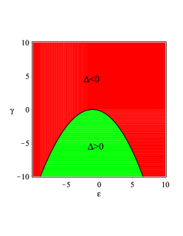
(a) $Q=0.2$

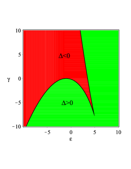
(b) $Q=0.5$

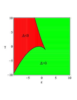
(c) $Q=0.8$

Figure 1: Positive or negative regions of discriminant $\Delta$ for $M=1$.

$$\Delta=\frac{p^{3}}{27}+\frac{q^{2}}{4},$$ (18)

with $p$ and $q$ defined by

$$p = -\frac{6M}{\gamma}-\frac{4}{3}\frac{(1+\varepsilon)^{2}}{\gamma^{2}},$$ (19)

$$q = \frac{4Q^{2}}{\gamma}+\frac{4M(1+\varepsilon)}{\gamma^{2}}+\frac{16}{27}\frac{(1+\varepsilon)^{3}}{\gamma^{3}}.$$ (20)

Depending on the values of the BH parameters, $\Delta$ can be positive or negative. In order to have a more precise picture, we have distinguished regions with negative/positive $\Delta$ in Fig. 1.

If $\Delta>0$, in this case there is only one real solution given by

$$r_{ph}=\left(-\frac{q}{2}+\sqrt{\Delta}\right)^{\frac{1}{3}}+\left(-\frac{q}{2}-\sqrt{\Delta}\right)^{\frac{1}{3}}-\frac{2}{3}\frac{(1+\varepsilon)}{\gamma}.$$ (21)

If $\Delta<0$, three real solutions exist in this case which are determined as follows

$$r_{ph}^{(1)} = \frac{2\sqrt{-p}}{\sqrt{3}}\sin\left[\frac{1}{3}\sin^{-1}\left(\frac{3\sqrt{3}q}{2(\sqrt{-p})^{3}}\right)\right]-\frac{2}{3}\frac{(1+\varepsilon)}{\gamma},$$ (22)

$$r_{ph}^{(2)} = -\frac{2\sqrt{-p}}{\sqrt{3}}\sin\left[\frac{1}{3}\sin^{-1}\left(\frac{3\sqrt{3}q}{2(\sqrt{-p})^{3}}\right)+\frac{\pi}{3}\right]-\frac{2}{3}\frac{(1+\varepsilon)}{\gamma},$$ (23)

$$r_{ph}^{(3)} = \frac{2\sqrt{-p}}{\sqrt{3}}\cos\left[\frac{1}{3}\sin^{-1}\left(\frac{3\sqrt{3}q}{2(\sqrt{-p})^{3}}\right)+\frac{\pi}{6}\right]-\frac{2}{3}\frac{(1+\varepsilon)}{\gamma}.$$ (24)

Our analysis shows that $r^{(2)}_{ph}$ is always negative and $r^{(3)}_{ph}$ given by Eq. (24) is the largest positive root. From the definition of the shadow radius Perlick2015 , the size of BH shadow can be obtained as

$$r_{sh}=\frac{L_{p}}{E}=\frac{r_{ph}}{\sqrt{f(r_{ph})}}.$$ (25)

The shape of the shadow seen by an observer at spatial infinity can be obtained from the geodesics of the photons in the celestial coordinates $x$ and $y$ as follows Vazquez1g

$$x = \lim_{r_{0}\rightarrow\infty}\left(-r_{0}^{2}\sin\theta_{0}\frac{d\varphi}{dr}\Big{|}_{(r_{0},\theta_{0})}\right),$$ (26)

$$y = \lim_{r_{0}\rightarrow\infty}\left(r_{0}^{2}\frac{d\theta}{dr}\Big{|}_{(r_{0},\theta_{0})}\right),$$

where $r_{0}$ is the distance between the observer and the BH, and $\theta_{0}$ is the inclination angle. For our solution, we obtain that

$$x=-\frac{r_{sh}}{\sqrt{1+\frac{\Lambda}{3}r_{sh}^{2}}},~{}~{}~{}~{}y=0,$$ (27)

It should be noted though the celestial coordinates are well defined for $r_{0}\longrightarrow\infty$ in our work, there are some cases where the celestial coordinates are not well defined in such a limit. For such cases, one can consider an observer at ”$r_{0}=$ constant” to determine the shape of a shadow (see Refs. Perlick2018 ; Grenzebach1a for more details).

Table 1: The event horizon ($r_{e}$), photon sphere radius ($r_{ph}$) and shadow radius ($r_{sh}$) for the variation of $Q$, $\gamma$, $\varepsilon$ and $\Lambda$ for $M=1$.

$Q$	$0.2$	$0.4$	$0.6$	$0.9$
$r_{e}$ ($\gamma=\varepsilon=0.2$, $\Lambda=-0.1$)	$1.2989$	$1.2468$	$1.1445$	$0.69+0.2I$
$r_{ph}$ ($\gamma=\varepsilon=0.2$, $\Lambda=-0.1$)	$2.1005$	$2.0262$	$1.8855$	$1.3461$
$r_{sh}$ ($\gamma=\varepsilon=0.2$, $\Lambda=-0.1$)	$2.3138$	$2.2739$	$2.1975$	$1.9212$
$r_{ph}>r_{e}$	✓	✓	✓	$\times$
$r_{sh}>r_{ph}$	✓	✓	✓	✓
$\gamma$	$-0.1$	$0.2$	$0.3$	$0.4$
$r_{e}$ ($Q=\varepsilon=0.2$, $\Lambda=-0.1$)	$1.7541$	$1.2989$	$1.2181$	$1.1524$
$r_{ph}$ ($Q=\varepsilon=0.2$, $\Lambda=-0.1$)	$2.5037$	$2.1005$	$1.9774$	$1.8771$
$r_{sh}$ ($Q=\varepsilon=0.2$, $\Lambda=-0.1$)	$8.5704$	$2.3138$	$2.0589$	$1.8639$
$r_{ph}>r_{e}$	✓	✓	✓	✓
$r_{sh}>r_{ph}$	✓	✓	✓	$\times$
$\varepsilon$	$-0.4$	$-0.1$	$0.6$	$1.5$
$r_{e}$ ($Q=\gamma=0.2$, $\Lambda=-0.1$)	$1.8336$	$1.5353$	$1.0608$	$0.7047$
$r_{ph}$ ($Q=\gamma=0.2$, $\Lambda=-0.1$)	$3.2614$	$2.5667$	$1.6706$	$1.0804$
$r_{sh}$ ($Q=\gamma=0.2$, $\Lambda=-0.1$)	$3.0224$	$2.7680$	$1.8181$	$1.0603$
$r_{ph}>r_{e}$	✓	✓	✓	✓
$r_{sh}>r_{ph}$	$\times$	✓	✓	$\times$
$\Lambda$	$0.01$	$-0.04$	$-0.1$	$-0.21$
$r_{e}$ ($Q=\gamma=\varepsilon=0.2$)	$65.36$	$1.3236$	$1.2989$	$1.2626$
$r_{ph}$ ($Q=\gamma=\varepsilon=0.2$)	$2.1005$	$2.1005$	$2.1005$	$2.1005$
$r_{sh}$ ($Q=\gamma=\varepsilon=0.2$)	$2.5810$	$2.4486$	$2.3138$	$2.0999$
$r_{ph}>r_{e}$	$\times$	✓	✓	✓
$r_{sh}>r_{ph}$	✓	✓	✓	$\times$

In order to observe an acceptable optical behavior, we need to investigate the condition $r_{e}<r_{ph}<r_{sh}$, where $r_{e}$ is radius related to the event horizon. It helps us find admissible regions of $\gamma$ and $\varepsilon$ for having an acceptable physical result. For clarity, we list several values of the event horizon, the photon sphere radius, and shadow radius in table 1. As one can see, the increase of the electric charge leads to an imaginary event horizon, indicating that an acceptable optical result can be observed only for limited regions of this parameter. Regarding the effects of the cosmological constant and massive parameters $\gamma$ and $\varepsilon$, we notice that for large values of these parameters, the shadow size is smaller than the photon sphere radius which is not acceptable physically. As a remarkable point regarding the parameter $\gamma$, we find that for negative values of this parameter, the shadow radius becomes too large compared to the size of the photon sphere radius ($r_{sh}\gg r_{ph}$). It reveals the fact that just for positive values of $\gamma$, one can obtain acceptable results. From this table, one can also find that the electric charge and massive parameters $\gamma$ and $\varepsilon$ have decreasing effects on the event horizon, photon sphere radius, and shadow size. Studying the effect of the cosmology constant, we find that increasing this parameter leads to decreasing the event horizon and shadow radii. Besides, it is clear that the cosmological constant does not affect the photon sphere radius. It is worth mentioning that according to our calculations, no acceptable optical behavior is observed in dS spacetime. To have a precise picture of the influence of these parameters on the shadow size, we have plotted Fig. 2. From this figure, one can find that massive parameters have a significant effect on the size of the black hole shadow compared to the electric charge and the cosmological constant parameters.

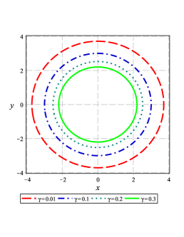
(a) $Q=\varepsilon=0.2$ and $\Lambda=-0.01$

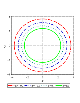
(b) $Q=\gamma=0.2$ and $\Lambda=-0.01$

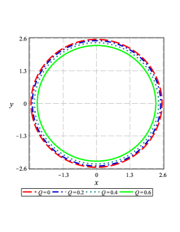
(c) $\gamma=\varepsilon=0.2$ and $\Lambda=-0.01$

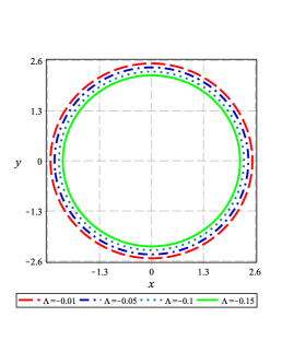
(d) $Q=\gamma=\varepsilon=0.2$

Figure 2: The BH shadow in the celestial plane $(x-y)$ for $M=1$.

II.2 Energy emission

Having the BH shadow, one can investigate the emission of particles around the BH. It was shown that the BH shadow corresponds to its high energy absorption cross-section for a far distant observer Wei2013 . In general, for a spherically symmetric BH, the absorption cross-section oscillates around a limiting constant value $\sigma_{lim}$ in the limit of very high energies. Since the shadow measures the optical appearance of a BH, it is approximately equal to the area of the photon sphere ($\sigma_{lim}\approx\pi r_{sh}^{2}$). The energy emission rate is obtained as

$$\frac{d^{2}\mathcal{E}(\omega)}{dtd\omega}=\frac{2\pi^{3}\omega^{3}r_{sh}^{2}}{e^{\frac{\omega}{T}}-1},$$ (28)

in which $\omega$ is the emission frequency, and $T$ is Hawking temperature given by

$$T=\frac{-\Lambda r_{e}^{4}+2\gamma r_{e}^{3}+(1+\varepsilon)r_{e}^{2}-Q^{2}}{4\pi r_{e}^{3}},$$ (29)

Figure 3, displays the behavior of energy emission rate as a function of $\omega$. As it is transparent, there exists a peak of the energy emission rate, which decreases and shifts to low frequencies as the parameters $\gamma$ and $\varepsilon$ decrease. Increasing these parameters leads to a fast emission of particles. Regarding the effect of electric charge, as we see from Fig. 3(c), this parameter decreases the energy emission so that when the BH is located in a weak electric field, the evaporation process would be faster. Studying the impact of the cosmological constant, we observe that $|\Lambda|$ has a decreasing effect on this optical quantity like the electric charge (see Fig. 3(d)). Therefore, one can find that the black hole has a longer lifetime in a high curvature background or with a strong electric field.

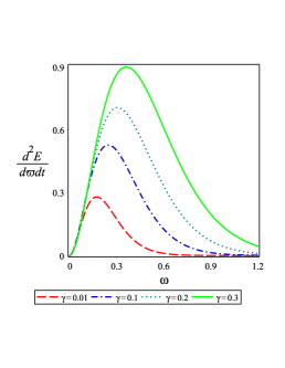
(a) $Q=\varepsilon=0.2$ and $\Lambda=-0.01$

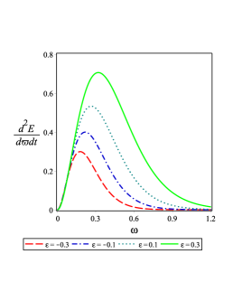
(b) $Q=\gamma=0.2$ and $\Lambda=-0.01$

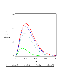
(c) $\gamma=\varepsilon=0.2$ and $\Lambda=-0.01$

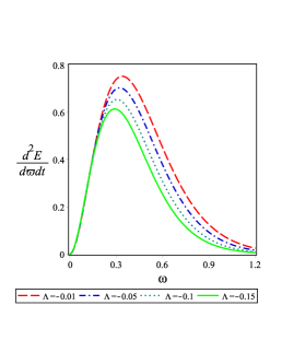
(d) $Q=\gamma=\varepsilon=0.2$

Figure 3: The energy emission rate versus $\omega$ for the corresponding BH with $M=1$ and different values of $\gamma$, $\varepsilon$, $Q$ and $\Lambda$.

III Rotating charged BH in dRGT massive gravity

In this section, we would like to generalize the spherically symmetric charged BH solution in dRGT massive gravity to the Kerr-like rotational BH solution by employing the Newman-Janis algorithm (NJA), which was first proposed by Newman and Janis in 1965 Newman1965 . This method has been widely used to construct rotating BH solutions from their non-rotating counterparts xu2017kerr ; kim2020rotating . In particular, it has been more recently applied to non-rotating solutions in modified gravity theories jusufi2020rotating ; Ghosh1ah . In GR, if a source exists, it is the same for both non-rotating BH and its rotating counterpart, e.g., charge for Reissner-Nordström and Kerr-Newman BHs. However, in the modified gravity, rotating BH counterparts obtained using NJA, in addition to original sources likely have additional sources. In this work, we will adopt the NJA modified by Azreg-Aïnou azreg2014generating ; azreg2014static , which can generate rotating solutions without complication.

First, we consider the general static and spherically symmetric metric

$$\text{d}s^{2}=-f(r)\text{d}t^{2}+g(r)^{-1}\text{d}r^{2}+h(r)\text{d}\Omega^{2}.$$ (30)

Then, we transform the metric (30) from the Boyer-Lindquist (BL) coordinates ($t,r,\theta,\varphi$) to the Eddington-Finkelstein (EF) coordinates ($u,r,\theta,\varphi$). This can be achieved by using the following coordinate transformation

$$\text{d}u=\text{d}t-\frac{\text{d}r}{\sqrt{f(r)g(r)}}.$$ (31)

So, the line element (30) takes the form

$$\text{d}s^{2}=-f\left(r\right)\text{d}u^{2}-2\sqrt{\frac{f\left(r\right)}{g\left(r\right)}}\text{d}u\text{d}r+h\left(r\right)\left(\text{d}\theta^{2}+\sin^{2}{\theta}\text{d}\varphi^{2}\right).$$ (32)

This metric can be decomposed in terms of null tetrad formalism as

$$g^{\mu\nu}=-l^{\mu}n^{\nu}-l^{\nu}n^{\mu}+m^{\mu}\bar{m}^{\nu}+m^{\nu}\bar{m}^{\mu},$$ (33)

where

$$\begin{gathered}l^{\mu}=\delta^{\mu}_{r},\qquad n^{\mu}=\sqrt{\frac{g\left(r\right)}{f\left(r\right)}}\delta^{\mu}_{0}-\frac{f\left(r\right)}{2}\delta^{\mu}_{r},\\ m^{\mu}=\frac{1}{\sqrt{2h\left(r\right)}}\delta^{\mu}_{\theta}+\frac{i}{\sqrt{2h\left(r\right)}\sin{\theta}}\delta^{\mu}_{\varphi},\quad\bar{m}^{\mu}=\frac{1}{\sqrt{2h\left(r\right)}}\delta^{\mu}_{\theta}-\frac{i}{\sqrt{2h\left(r\right)}\sin{\theta}}\delta^{\mu}_{\varphi}.\end{gathered}$$ (34)

These vectors further satisfy the conditions for normalization, orthogonality and isotropy as

$$\begin{gathered}l^{\mu}l_{\mu}=n^{\mu}n_{\mu}=m^{\mu}m_{\mu}=\bar{m}^{\mu}\bar{m}_{\mu}=0,\\ l^{\mu}m_{\mu}=n^{\mu}m_{\mu}=l^{\mu}\bar{m}_{\mu}=n^{\mu}\bar{m}_{\mu}=0,\\ l^{\mu}n_{\mu}=-m^{\mu}\bar{m}_{\mu}=1.\end{gathered}$$ (35)

Now, we consider complex coordinate transformations as follows

$${x^{\prime}}^{\mu}=x^{\mu}+ia(\delta_{r}^{\mu}-\delta_{u}^{\mu})\cos\theta\rightarrow\\ \left\{\begin{array}[]{ll}u^{\prime}=u-ia\cos\theta,\\ r^{\prime}=r+ia\cos\theta,\\ \theta^{\prime}=\theta,\\ \varphi^{\prime}=\varphi.\end{array}\right.$$ (36)

We assume that the metric functions take a new form under these transformations as: $f\left(r\right)\rightarrow F\left(r,a,\theta\right)$, $g\left(r\right)\rightarrow G\left(r,a,\theta\right)$, and $h\left(r\right)\rightarrow\Sigma=r^{2}+a^{2}\cos^{2}{\theta}$ azreg2014generating ; azreg2014static . So, null tetrad basis may take the new form

$$\begin{split}l^{\prime\mu}&=\delta^{\mu}_{r},\quad n^{\prime\mu}=\sqrt{\frac{G}{F}}\delta^{\mu}_{0}-\frac{1}{2}F\delta^{\mu}_{r},\\ m^{\prime\mu}&=\frac{1}{\sqrt{2\Sigma}}\left(\delta^{\mu}_{\theta}+ia\sin{\theta}\left(\delta^{\mu}_{0}-\delta^{\mu}_{r}\right)+\frac{i}{\sin{\theta}}\delta^{\mu}_{\varphi}\right),\\ \bar{m}^{\prime\mu}&=\frac{1}{\sqrt{2\Sigma}}\left(\delta^{\mu}_{\theta}-ia\sin{\theta}\left(\delta^{\mu}_{0}-\delta^{\mu}_{r}\right)-\frac{i}{\sin{\theta}}\delta^{\mu}_{\varphi}\right).\end{split}$$ (37)

Using Eq. (33), the contravariant components of the metric $g^{\mu\nu}$ is obtained as

$$\begin{split}g^{uu}&=\frac{a^{2}\sin^{2}{\theta}}{\Sigma},\quad g^{rr}=G+\frac{a^{2}\sin^{2}{\theta}}{\Sigma},\\ g^{\theta\theta}&=\frac{1}{\Sigma},\quad g^{\varphi\varphi}=\frac{1}{\Sigma\sin^{2}{\theta}},\\ g^{ur}&=g^{ru}=-\sqrt{\frac{G}{F}}-\frac{a^{2}\sin^{2}{\theta}}{\Sigma},\\ g^{u\varphi}&=g^{\varphi u}=\frac{a}{\Sigma},\quad g^{r\varphi}=g^{\varphi r}=-\frac{a}{\Sigma}.\end{split}$$ (38)

The new metric is found as follows

$$\begin{split}\mathrm{d}s^{2}=&-F\mathrm{d}u^{2}-2\sqrt{\frac{F}{G}}\mathrm{d}u\mathrm{d}r+2a\left(F-\sqrt{\frac{F}{G}}\right)\sin^{2}{\theta}\mathrm{d}u\mathrm{d}\varphi+\Sigma\mathrm{d}\theta^{2}\\ &+2a\sin^{2}{\theta}\sqrt{\frac{F}{G}}\mathrm{d}r\mathrm{d}\varphi+\sin^{2}{\theta}\left[\Sigma+a^{2}\left(2\sqrt{\frac{F}{G}}-F\right)\sin^{2}{\theta}\right]\mathrm{d}\varphi^{2}.\end{split}$$ (39)

Now, we revert Eq (39) back to BL coordinates by using the following transformation

$$\mathrm{d}u=\mathrm{d}t+\lambda\left(r\right)\mathrm{d}r,\quad\mathrm{d}\varphi=\mathrm{d}\phi+\chi\left(r\right)\mathrm{d}r,$$ (40)

where

$$\lambda\left(r\right)=-\frac{k(r)+a^{2}}{g\left(r\right)h\left(r\right)+a^{2}},\quad\chi\left(r\right)=-\frac{a}{g\left(r\right)h\left(r\right)+a^{2}},\quad k\left(r\right)=\sqrt{\frac{g\left(r\right)}{f\left(r\right)}}h\left(r\right),$$ (41)

with

$$F\left(r,\theta\right)=\frac{\left(g(r)h(r)+a^{2}\cos^{2}{\theta}\right)\Sigma}{\left(k(r)^{2}+a^{2}\cos^{2}{\theta}\right)^{2}},\quad G\left(r,\theta\right)=\frac{g(r)h(r)+a^{2}\cos^{2}{\theta}}{\Sigma}.$$ (42)

Hence the rotating counterpart corresponding to the metric (30) turns out to be

$$\begin{split}\mathrm{d}s^{2}=&-\frac{\left(g(r)h(r)+a^{2}\cos^{2}{\theta}\right)\Sigma}{\left(k(r)+a^{2}\cos^{2}{\theta}\right)^{2}}\mathrm{d}t^{2}+\frac{\Sigma}{g(r)h(r)+a^{2}}\mathrm{d}r^{2}-2a\sin^{2}\theta\left[\frac{k(r)-g(r)h(r)}{\left(k(r)+a^{2}\cos^{2}{\theta}\right)^{2}}\right]\Sigma\mathrm{d}\phi\mathrm{d}t\\ &+\Sigma\mathrm{d}\theta^{2}+\Sigma\sin^{2}\theta\left[1+a^{2}\sin^{2}\theta\frac{2k(r)-g(r)h(r)+a^{2}\cos^{2}\theta}{\left(k(r)+a^{2}\cos^{2}{\theta}\right)^{2}}\right]\mathrm{d}\phi^{2}.\end{split}$$ (43)

Comparing the line elements (7) with (30), one finds $f(r)=g(r)$ and $h(r)=k(r)=r^{2}$. Finally, we obtain the metric of charged rotating BHs in dRGT massive gravity in the form

$$\begin{split}\mathrm{d}s^{2}=&-\left(1-\frac{2\rho r}{\Sigma}\right)\mathrm{d}t^{2}+\frac{\Sigma}{\Delta_{r}}\mathrm{d}r^{2}+\Sigma\mathrm{d}\theta^{2}-\frac{4a\rho r\sin^{2}{\theta}}{\Sigma}\mathrm{d}t\mathrm{d}\phi\\ &+\sin^{2}{\theta}\left(r^{2}+a^{2}+\frac{2a^{2}\rho r\sin^{2}{\theta}}{\Sigma}\right)\mathrm{d}\phi^{2},\end{split}$$ (44)

with

$$\begin{gathered}\Delta_{r}=r^{2}+a^{2}-2Mr+Q^{2}-\frac{\Lambda}{3}r^{4}+\gamma r^{3}+\varepsilon r^{2},\\ 2\rho=2M-\frac{Q^{2}}{r}+\frac{\Lambda}{3}r^{3}-\gamma r^{2}-\varepsilon r,\\ \Sigma=r^{2}+a^{2}\cos^{2}{\theta}.\end{gathered}$$ (45)

III.1 Null geodesics

In order to find the contour of a BH shadow related to the rotating spacetime metric (44), we need to separate the null geodesic equations using the Hamilton-Jacobi equation given by

$$\frac{\partial S}{\partial\sigma}=-\frac{1}{2}g^{\mu\nu}\frac{\partial S}{\partial x^{\mu}}\frac{\partial S}{\partial x^{\nu}},$$ (46)

where $S$ and $\sigma$ are the Jacobi action and affine parameter along the geodesics, respectively. Using known constants of the motion, one can separate the Jacobi function as follows

$$S=-\frac{1}{2}\mu^{2}\sigma+Et-L\phi+S_{r}(r)+S_{\theta}(\theta),$$ (47)

where $\mu$ is the mass of the test particle, $E=p_{t}$ and $L=p_{\phi}$ are, respectively, the conserved energy and angular momentum. The functions $S_{r}(r)$ and $S_{\theta}(\theta)$ respectively depends on coordinates $r$ and $\theta$. Combining Eq. (46) and Eq. (47) and applying the variable separable method, we get the null geodesic equations for a moving photon ($\mu=0$) around the rotating BH in dRGT massive gravity as

$$\Sigma\frac{dt}{d\sigma}=\frac{r^{2}+a^{2}}{\Delta_{r}}[E(r^{2}+a^{2})-aL]-a(aE\sin^{2}\theta-L),$$ (48)

$$\Sigma\frac{dr}{d\sigma}=\sqrt{\mathcal{R}(r)},$$ (49)

$$\Sigma\frac{d\theta}{d\sigma}=\sqrt{\Theta(\theta)},$$ (50)

$$\Sigma\frac{d\phi}{d\sigma}=\frac{a}{\Delta_{r}}[E(r^{2}+a^{2})-aL]-\left(aE-\frac{L}{\sin^{2}\theta}\right),$$ (51)

where $\mathcal{R}(r)$ and $\Theta(\theta)$ read as

$$\mathcal{R}(r)=[E(r^{2}+a^{2})-aL]^{2}-\Delta_{r}[(aE-L)^{2}+\mathcal{K}],$$ (52)

$$\Theta(\theta)=\mathcal{K}-\left(\dfrac{L^{2}}{\sin^{2}\theta}-a^{2}E^{2}\right)\cos^{2}\theta,$$ (53)

with $\mathcal{K}$ the Carter constant. For $\mathcal{K}=0$, $\theta$-motion is suppressed, and all photon orbits are restricted only to a plane ($\theta=\pi/2$), yielding unstable circular orbits at the equatorial plane. In order to obtain the size and shape of the BH shadow, we need to express the radial geodesic equation in terms of the effective potential $V_{\text{eff}}$ as

$$\Sigma^{2}\left(\frac{dr}{d\sigma}\right)^{2}+V_{\text{eff}}=0.$$

Introducing two impact parameters $\xi$ and $\eta$ Chandrasekhar1g as

$$\xi=L/E,\;\;\;\;\;\;\eta=\mathcal{K}/E^{2}.$$ (54)

The effective potential $V_{\text{eff}}$ reads

$$V_{\text{eff}}=\Delta_{r}((a-\xi)^{2}+\eta)-(r^{2}+a^{2}-a\;\xi)^{2},$$ (55)

where we have replaced $V_{\text{eff}}/E^{2}$ by $V_{\text{eff}}$. The boundary of the shadow is mainly determined by the circular photon orbit, which satisfies the following conditions

$$V_{\text{eff}}(r_{ph})=0,\quad~{}~{}~{}\frac{dV_{\text{eff}}(r_{ph})}{dr}=0,$$ (56)

whereas instability of orbits obeys condition

$$\frac{d^{2}V_{\text{eff}}(r_{ph})}{dr^{2}}<0,$$ (57)

Solving Eq. (56), the critical values of impact parameters for photons unstable orbits read

$$\xi_{c} = \frac{(r_{ph}^{2}+a^{2})\Delta^{\prime}(r_{ph})-4r_{ph}\Delta(r_{ph})}{a\Delta^{\prime}(r_{ph})},$$ (58)

$$\eta_{c} = \frac{r_{ph}^{2}\left[16a^{2}\Delta(r_{ph})+8r_{ph}\Delta(r_{ph})\Delta^{\prime}(r_{ph})-16\Delta(r_{ph})^{2}-r_{ph}^{2}\Delta^{\prime}(r_{ph})^{2}\right]}{a^{2}\Delta^{\prime}(r_{ph})^{2}}.$$ (59)

Table 2: The event horizon ($r_{e}$), photon sphere radius ($r_{ph}$) and shadow radius ($r_{sh}$) for the variation of $Q$, $a$, $\gamma$, $\varepsilon$ and $\Lambda$ for $M=1$ and $\theta_{0}=0$.

$Q$	$0.1$	$0.3$	$0.5$	$0.7$
$r_{e}$ ($a=0.5$, $\varepsilon=0.5$, $\gamma=0.2$, $\Lambda=-0.01$)	$1.0228$	$0.9721$	$0.8414$	$0.59+0.25I$
$r_{ph}$ ($a=0.5$, $\varepsilon=0.5$, $\gamma=0.2$, $\Lambda=-0.01$)	$1.7395$	$1.6833$	$1.5535$	$1.2523$
$r_{sh}$ ($a=0.5$, $\varepsilon=0.5$, $\gamma=0.2$, $\Lambda=-0.01$)	$2.1132$	$2.0768$	$1.9949$	$1.8285$
$r_{ph}>r_{e}$	✓	✓	✓	$\times$
$r_{sh}>r_{ph}$	✓	✓	✓	✓
$a$	$0.1$	$0.3$	$0.5$	$0.7$
$r_{e}$ ($Q=0.5$, $\varepsilon=0.5$, $\gamma=0.2$, $\Lambda=-0.01$)	$1.0228$	$0.9721$	$0.8414$	$0.59+0.25I$
$r_{ph}$ ($Q=0.5$, $\varepsilon=0.5$, $\gamma=0.2$, $\Lambda=-0.01$)	$1.6170$	$1.5975$	$1.5535$	$1.4674$
$r_{sh}$ ($Q=0.5$, $\varepsilon=0.5$, $\gamma=0.2$, $\Lambda=-0.01$)	$1.9474$	$1.9637$	$1.9949$	$2.0378$
$r_{ph}>r_{e}$	✓	✓	✓	$\times$
$r_{sh}>r_{ph}$	✓	✓	✓	✓
$\gamma$	$0.1$	$0.3$	$0.5$	$0.7$
$r_{e}$ ($a=Q=0.5$, $\varepsilon=0.5$, $\Lambda=-0.01$)	$0.9102$	$0.7842$	$0.6910$	$0.6139$
$r_{ph}$ ($a=Q=0.5$, $\varepsilon=0.5$, $\Lambda=-0.01$)	$1.6184$	$1.4998$	$1.4151$	$1.3764$
$r_{sh}$ ($a=Q=0.5$, $\varepsilon=0.5$, $\Lambda=-0.01$)	$2.2413$	$1.8116$	$1.5529$	$1.3509$
$r_{ph}>r_{e}$	✓	✓	✓	✓
$r_{sh}>r_{ph}$	✓	✓	✓	$\times$
$\varepsilon$	$-1.2$	$-0.5$	$0.5$	$1$
$r_{e}$ ($a=Q=0.5$, $\gamma=0.2$, $\Lambda=-0.01$)	$3.4719$	$1.9359$	$0.8414$	$0.4+0.09I$
$r_{ph}$ ($a=Q=0.5$, $\gamma=0.2$, $\Lambda=-0.01$)	$6.7261$	$3.3498$	$1.5535$	$1.1639$
$r_{sh}$ ($a=Q=0.5$, $\gamma=0.2$, $\Lambda=-0.01$)	$6.3948$	$4.2316$	$1.9949$	$1.4630$
$r_{ph}>r_{e}$	✓	✓	✓	$\times$
$r_{sh}>r_{ph}$	$\times$	✓	✓	✓
$\Lambda$	$-0.01$	$-0.1$	$-0.2$	$-0.4$
$r_{e}$ ($a=Q=0.5$, $\gamma=0.2$, $\varepsilon=0.5$)	$0.8414$	$0.8263$	$0.8108$	$0.7832$
$r_{ph}$ ($a=Q=0.5$, $\gamma=0.2$, $\varepsilon=0.5$)	$1.5535$	$1.5701$	$1.5887$	$1.6692$
$r_{sh}$ ($a=Q=0.5$, $\gamma=0.2$, $\varepsilon=0.5$)	$1.9949$	$1.9036$	$1.8152$	$1.6267$
$r_{ph}>r_{e}$	✓	✓	✓	✓
$r_{sh}>r_{ph}$	✓	✓	✓	$\times$

Using Eq. (26) and the null geodesic equations (48)-(51), we get the relations between celestial coordinates and impact parameters as

$$x=\frac{a\sin\theta_{0}-\xi\csc\theta_{0}}{\sqrt{1+\frac{\Lambda}{3}\left[(a-\xi)^{2}+\eta\right]}}\,,\qquad y=\pm\sqrt{\frac{\eta+a^{2}\cos^{2}\theta_{0}-\xi^{2}\cot^{2}\theta_{0}}{1+\frac{\Lambda}{3}\left[(a-\xi)^{2}+\eta\right]}}\,.$$ (60)

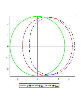
(a) $Q=\gamma=\varepsilon=0.2$, $a=0.8$ and $\Lambda=-0.01$

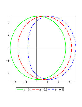
(b) $Q=\gamma=\varepsilon=0.2$, $\Lambda=-0.01$ and $\theta_{0}=\pi/2$

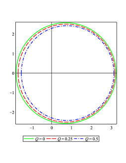
(c) $a=0.5$, $\gamma=\varepsilon=0.2$, $\Lambda=-0.01$ and $\theta_{0}=\pi/2$

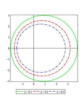
(d) $Q=\varepsilon=0.2$, $a=0.5$, $\Lambda=-0.01$ and $\theta_{0}=\pi/2$

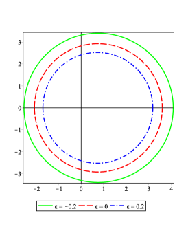
(e) $Q=\gamma=0.2$, $a=0.5$, $\Lambda=-0.01$ and $\theta_{0}=\pi/2$

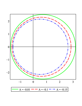
(f) $Q=\gamma=\varepsilon=0.2$, $a=0.5$ and $\theta_{0}=\pi/2$

Figure 4: Shadow cast by a charged rotating BH in dRGT massive gravity with $M=1$ and different values of $\theta_{0}$, $a$, $Q$, $\gamma$, $\varepsilon$ and $\Lambda$.

In the present paper, we shall use the definition adopted in Ref. Feng1g . According to Eq. (60), the shape of the shadow depends on the observer’s viewing angle $\theta_{0}$. For north pole $\theta_{0}=0$ (or equivalent south pole $\theta_{0}=\pi$) the shadow remains a round disk. In this case, the photons forming the shadow boundary satisfy

$$\xi(r^{0}_{\rm ph})=0\,,$$ (61)

and the shadow radius is

$$R_{\rm sh}=\sqrt{\frac{a^{2}+\eta(r^{0}_{\rm ph})}{1+\frac{\Lambda}{3}\left[a^{2}+\eta(r^{0}_{\rm ph})\right]}}.$$ (62)

When $\theta_{0}\neq 0$ or $\pi$, the shadows are no longer round but distorted. The maximum distortion occurs for $\theta_{0}=\pi/2$ in the equatorial plane. For this case, the vertical $y$-direction is elongated while the horizontal $x$-direction is squeezed, but the shadows remain convex. For $y=0$, there are two real solutions

$$\eta(r_{\rm ph}^{\pm})=0\,,\qquad\hbox{with}\qquad r_{\rm ph}^{+}\geq r_{\rm ph}^{-}$$ (63)

The size of the shadow is defined as

$$R_{\rm sh}=\frac{1}{2}\big{(}x(r_{\rm ph}^{+})-x(r_{\rm ph}^{-})\big{)}\,.$$ (64)

For general $\theta_{0}$, one can determine $r_{\rm ph}^{\pm}$ by requiring

$$y(r,\theta_{0})\Big{|}_{r=r_{\rm ph}^{\pm}}=0\,,$$ (65)

and the shadow size is then again formally given by (64).

Here, we are interested in investigating the allowed region to observe acceptable optical behavior for the rotating BH in dRGT massive gravity. To do so, we have listed several values of the event horizon, photon sphere radius, and shadow radii in table 2. As we see, similar to the non-rotating case, an acceptable optical result can be obtained just for limited regions of the electric charge, rotation parameter, cosmological constant, and massive parameters $\gamma$ and $\varepsilon$. As a significant point related to the effects of $Q$, $a$, and $\varepsilon$, we should note that as these parameters increase, some constraints are imposed on them due to the imaginary event horizon. Regarding the influence of the cosmological constant and the parameter $\gamma$ on the admissible region, our findings show that increasing these two parameters leads to a non-physical result $\frac{r_{sh}}{r_{ph}}<1$. This table also helps us find the impact of the black hole parameters on the size of the event horizon and photon sphere. As we see, all parameters except the cosmological constant have a decreasing effect on the event horizon and photon sphere radius. Although the cosmological constant has a decreasing contribution to the event horizon similar to other parameters, its contribution to the photon sphere radius is opposite.

In Fig. 4, different shapes of the shadow are obtained by plotting $y$ against $x$ using Eq. (60). Figs. 4(a) and 4(b) display the effects of angle $\theta_{0}$ and rotation parameter $a$ on the shadow shape. It is evident that deformation in shapes of the shadow gets more significant with the increasing $\theta_{0}$ and $a$. Regarding the impacts of electric charge and parameters $\gamma$ and $\varepsilon$ on the radius of shadow, we see that the shadow size shrinks with increasing of electric charge (see Fig. 4(c)) and massive parameters $\gamma$ and $\varepsilon$ (see Figs. 4(d) and 4(e)). To study the impact of the cosmological constant on the black hole shadow, we have plotted Fig. 4(f), indicating that increasing $|\Lambda|$ makes the decreasing of the shadow radius. Furthermore, we find that variation of $Q$ has a weaker effect on the shadow size than the massive parameters.

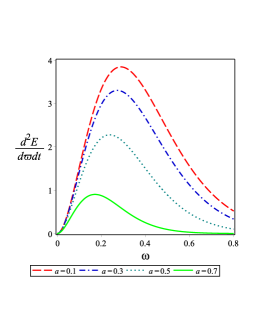
(a) $Q=\gamma=\varepsilon=0.2$ and $\Lambda=-0.01$

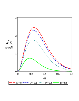
(b) $a=0.5$, $\gamma=\varepsilon=0.2$ and $\Lambda=-0.01$

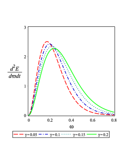
(c) $a=0.5$, $Q=\varepsilon=0.2$ and $\Lambda=-0.01$

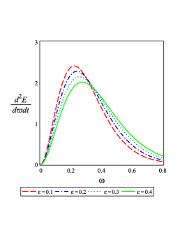
(d) $Q=\gamma=0.2$, $a=0.5$ and $\Lambda=-0.01$

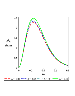
(e) $Q=\gamma=\varepsilon=0.2$ and $a=0.5$

Figure 5: Evolution of the BH energy emission rate with the frequency $\omega$ for $M=1$ and different values of $a$, $Q$, $\gamma$, $\varepsilon$ and $\Lambda$.

III.2 Energy emission rate

As it was already mentioned, for an observer located at infinity, the BH shadow corresponds to the high energy absorption cross-section of the BH, which oscillates around a constant limiting value $\sigma_{lim}\approx\pi R_{\text{sh}}^{2}$. In this subsection, we intend to extend this result to the rotating BH considered in this work. From the geometry of the shadow, the observable $R_{\text{sh}}$ which designates approximately the size of the shadow, can be expressed in the form

$$R_{\text{sh}}=\frac{(x_{t}-x_{r})^{2}+y_{t}^{2}}{2|x_{t}-x_{r}|}.$$ (66)

Equation (28) can be used to obtain the energy emission rate for a rotating BH as well. The Hawking temperature of the charged rotating BH in dRGT massive gravity at event horizon $r_{+}$ becomes

$$T=\frac{\Lambda r_{e}^{4}+2\gamma r_{e}^{3}+\varepsilon r_{e}^{2}-Q^{2}-a^{2}+r_{e}^{2}}{4\pi r_{e}(r_{e}^{2}+a^{2})}.$$ (67)

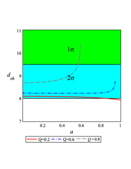
(a) $\gamma=0.02$, $\varepsilon=0.05$ and $\Lambda=-0.01$

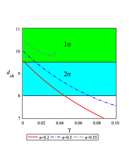
(b) $Q=0.8$, $\varepsilon=0.05$ and $\Lambda=-0.01$

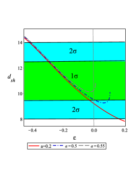
(c) $Q=0.8$, $\gamma=0.02$ and $\Lambda=-0.01$

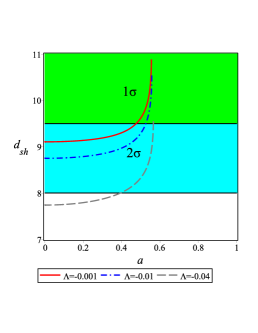
(d) $Q=0.8$, $\varepsilon=0.05$ and $\gamma=0.02$

Figure 6: Left-up graph: The predicted diameter for a charged rotating BH in dRGT massive gravity as a function of the rotation parameter for fixed $\gamma$, $\varepsilon$, $\Lambda$, and for several values of the electric charge. Right-up graph: $d_{sh}$ as a function of the parameter $\gamma$, for fixed $Q$, $\varepsilon$, $\Lambda$, and different values of the rotation parameter. Left-down graph: $d_{sh}$ as a function of the parameter $\varepsilon$, for fixed $Q$, $\gamma$, $\Lambda$, and different values of the rotation parameter. Right-down graph: $d_{sh}$ as a function of the rotation parameter, for fixed $Q$, $\varepsilon$, $\gamma$, and different values of the cosmological constant. The green shaded region gives the $1\sigma$ confidence region for $d_{sh}$, whereas the cyan shaded region gives the $2\sigma$ confidence region. The inclination angle is $\theta_{0}=0^{\circ}$.

In Fig. 5, we illustrate the behavior of the energy emission rate of the corresponding rotating BH against the photon frequency $\omega$ for various values of BH parameters. From Figs. 5(a) and 5(b), the emission rate peak decreases with an increase in $a$ and $Q$, and shifts to a lower value of $\omega$ with the increase of these two parameters. This reveals that the evaporation process would be slow for a fast-rotating BH or a BH located in a powerful electric field. Figures. 5(c) and 5(d) display the effective role of massive parameters $\gamma$ and $\varepsilon$ on this optical quantity. Based on these figures, although these parameters have a decreasing effect on the emission rate like the electric charge and rotation parameter, the peak of the energy emission rate shifts to a higher value of $\omega$ with the increase of $\gamma$ and $\varepsilon$. Taking a look at Fig. 5(e), one can find that the effect of the cosmological constant on the emission rate is opposite to that of the electric charge and rotation parameter. In other words, as $|\Lambda|$ increases, the emission of particles around the BH increases. From what we mentioned before, one can say that the BH will have a longer lifetime if it is located in a powerful electric field and low curvature background or if it rotates faster. Comparing Fig. 5 to Fig. 3, one can find that although the massive parameters have an increasing effect on the energy emission rate for static BHs in dRGT massive gravity, their contribution is to decrease the energy emission rate for rotating ones. It shows that the effect of these two parameters changes in the presence of the rotation parameter. Also, by comparing these two figures, one can notice that a static black hole in dRGT massive gravity has a longer lifetime if it is located in a high curvature background, whereas its lifetime becomes short in such a background by adding the rotation parameter to it.

IV Comparison with the EHT data

The EHT Collaboration has recently observed the shadow of the M87* BH residing at the center of nearby galaxy M87* using the very large baseline interferometry technique. In this section, we intend to compare the resulting shadow of the BHs with observational data to find the allowed regions of the model parameters for which the obtained shadow is consistent with the data. Since supermassive BHs are rotating, we study the rotating version of BHs in dRGT massive gravity to obtain more careful results. From Fig. 4, we deduce that the size of the resulting shadow is sensitive on the BH parameters, and hence the image of M87* can impose bounds on them. Here, we use the EHT constraints on the diameter of shadow to constrain the model’s parameters to be consistent with the M87* image within $1\sigma$ and $2\sigma$ confidence.

According to the obtained results by EHT collaboration Akiyama , the angular size of the shadow, the mass and the distance to M87* one respectively has the values

$$\delta = (42\pm 3)\mu as,$$ (68)

$$M = (6.5\pm 0.9)\times 10^{9}M_{\odot},$$ (69)

$$D = 16.8^{+0.8}_{-0.7}Mpc,$$ (70)

where $M_{\odot}$ is the Sun mass. These numbers imply that the diameter of the shadow in units of mass should be Bambi1dx

$$d_{M87^{*}}\equiv\frac{D\delta}{M}\approx 11.0\pm 1.5.$$ (71)

This combination can be used to confront the theoretically predicted shadows. As we see from Eq. (71), within $1\sigma$ uncertainty $9.5\lesssim d_{M87^{*}}\lesssim 12.5$ whereas within $2\sigma$ uncertainty $8.0\lesssim d_{M87^{*}}\lesssim 14.0$. In order to confront the rotating solution in dRGT massive gravity with the above observational number, we need to calculate the diameter of the predicted shadow.

Taking into account the allowed values of $d_{M87^{*}}$, we are in a position to compare the resulting shadow of charged rotating BHs in dRGT massive gravity with EHT data. We conduct our investigation for the inclination angle $\theta_{0}=0^{\circ}$, $90^{\circ}$ and $17^{\circ}$. It is worth pointing out that in agreement with EHT, it is better to consider the value $\theta_{0}=17^{\circ}$ for the inclination angle. In Fig. 6, we plot the diameter of the resulting shadow as a function of the rotation parameter $a$ and massive parameters $\varepsilon$ and $\gamma$ for the inclination angle $\theta_{0}=0^{\circ}$ together with $1\sigma$ and $2\sigma$ confidence intervals.

In Fig. 6(a), we see that for a more slowly rotating BH located in a weak electric field, the resulting shadow is consistent with observations within $2\sigma$-error, whereas for a fast-rotating BH in such a situation, the resulting shadow is not in agreement with EHT data (see the red solid curve of this figure). For intermediate values of the electric charge, $d_{sh}$ is located in $2\sigma$ confidence region for all values of the rotation parameter (see the blue dot-dash curve in Fig. 6(a)). For large electric charge, $d_{sh}$ becomes consistent with EHT data within $1\sigma$-error only for intermediate values of the rotation parameter, otherwise it is in agreement with observations in $2\sigma$ confidence region (see the gray dash curve in Fig. 6(a)). As a result, one can say that only in the presence of a powerful electric field, the shadow of such black holes is consistent with observational data within $1\sigma$-error. Fig. 6(b) displays the behavior of $d_{sh}$ with respect to parameter $\gamma$ for different values of the rotation parameter. According to our analysis, the resulting shadow becomes consistent with the detection of the Event Horizon Telescope in the region $0<\gamma<0.0445$ for slowly rotating BHs (see the red curve in Fig. 6(b)). For intermediate values of the rotation parameter, a compatible result will obtain for $\gamma<0.072$ (see the blue dot-dash curve in Fig. 6(b)). In the region of $0.55<a<0.59$, the black hole has a shadow in agreement with observational data within $1\sigma$-error (see the gray dash curve in Fig. 6(b)). As we see from Fig. 6(b), for too small values of the parameter $\gamma$, the resulting shadow of fast (slowly) rotating BHs is in agreement with observational data within $1\sigma$-error ($2\sigma$-error). In Fig. 6(c), we study the allowed region of the parameter $\varepsilon$ which is in agreement with EHT detection. Our investigation shows that for fast (slowly) rotating BHs the allowed region of this parameter is $-0.42<\varepsilon<0.01$ ($-0.42<\varepsilon<0.169$). As we see, in order to have consistent results with EHT data, it is better to consider negative $\varepsilon$ values. From this figure, one can also find that in the region $-0.3<\varepsilon<-0.03$, a rotating BH is in $1\sigma$ confidence region all the time. Fig. 6(e) displays the effective role of the cosmological constant on the allowed region. It can be seen that the black hole should be considered in a very low curvature background in order for the results to be consistent with the EHT data. In a high curvature background, only fast-rotating BHs have a shadow in agreement with observational data within the $2\sigma$-error (see the gray dash curve in Fig. 6(e)).

Table 3: The shadow diameter for the variation of the rotation parameter, the electric charge, the parameter $\gamma$ and $\varepsilon$ for $M=1$ and $\theta_{0}=\pi/2$.

$a$	$0.1$	$0.3$	$0.5$	$0.8$
$d_{sh}(Q=0.2$, $\gamma=0.02$, $\varepsilon=0.05$ and $\Lambda=-0.01$)	$8.6012$	$8.5443$	$8.4205$	$8.0187$
$Q$	$0.1$	$0.3$	$0.5$	$0.7$
$d_{sh}(a=0.1$, $\gamma=0.02$, $\varepsilon=0.05$ and $\Lambda=-0.01$)	$8.6424$	$8.5310$	$8.2939$	$7.8967$
$\gamma$	$0.01$	$0.02$	$0.04$	$0.05$
$d_{sh}(a=0.1$, $Q=0.2$, $\varepsilon=0.05$ and $\Lambda=-0.01$)	$8.9038$	$8.6012$	$8.0693$	$7.8339$
$\varepsilon$	$-0.25$	$-0.1$	$0.05$	$0.1$
$d_{sh}(a=0.1$, $Q=0.2$, $\gamma=0.02$ and $\Lambda=-0.01$)	$12.8262$	$10.4187$	$8.6012$	$8.0812$
$\Lambda$	$-0.001$	$-0.01$	$-0.03$	$-0.04$
$d_{sh}(a=0.1$, $Q=0.2$, $\gamma=0.02$ and $\varepsilon=0.05$)	$8.8515$	$8.6012$	$8.1132$	$7.8985$

Table 4: The shadow diameter for the variation of the rotation parameter, the electric charge, the parameter $\gamma$ and $\varepsilon$ for $M=1$ and $\theta_{0}=17^{\circ}$.

$a$	$0.1$	$0.3$	$0.5$	$0.9$
$d_{sh}(Q=0.2$, $\gamma=0.02$, $\varepsilon=0.05$ and $\Lambda=-0.01$)	$8.6052$	$8.5816$	$8.5298$	$8.2674$
$Q$	$0.1$	$0.3$	$0.5$	$0.7$
$d_{sh}(a=0.1$, $\gamma=0.02$, $\varepsilon=0.05$ and $\Lambda=-0.01$)	$8.6464$	$8.5352$	$8.2685$	$7.8969$
$\gamma$	$0.01$	$0.02$	$0.04$	$0.05$
$d_{sh}(a=0.1$, $Q=0.2$, $\varepsilon=0.05$ and $\Lambda=-0.01$)	$8.9072$	$8.6052$	$8.0743$	$7.8393$
$\varepsilon$	$-0.25$	$-0.1$	$0.05$	$0.1$
$d_{sh}(a=0.5$, $Q=0.2$, $\gamma=0.02$ and and $\Lambda=-0.01$)	$12.8308$	$10.4597$	$8.6052$	$8.1042$
$\Lambda$	$-0.001$	$-0.01$	$-0.03$	$-0.04$
$d_{sh}(a=0.1$, $Q=0.2$, $\gamma=0.02$ and $\varepsilon=0.05$)	$8.8541$	$8.6052$	$8.1197$	$7.9058$

We continue our investigation for the inclination angle $\theta_{0}=90^{\circ}$ and $17^{\circ}$. Since analytical method is not possible for these cases, we employ numerical method. The diameter of shadow for some parameters is listed in table 3 ($\theta_{0}=90^{\circ}$) and table 4 ($\theta_{0}=17^{\circ}$), thereby we understand the behavior of $d_{sh}$ under variation of the rotation parameter, electric charge, cosmological constant, parameters $\gamma$ and $\varepsilon$. In these two tables, we examine the allowed regions of the BH parameters within $1\sigma$/$2\sigma$ -error. For the inclination angle $\theta_{0}=90^{\circ}$, the resulting shadow of the charged rotating BH is in agreement with observations for values of $0<a<0.8$. Whereas for angle $\theta_{0}=17^{\circ}$, the allowed region of rotation parameter is $0<a<0.9$. Our findings show that for values of $-0.203<\varepsilon<-0.03$, the resulting shadow is in agreement with EHT data within $1\sigma$-error, whereas for values of $-031<\varepsilon<-0.203$ or $-0.03<\varepsilon<0.1$ the resulting shadow is consistent with EHT data within $2\sigma$-error.

V Conclusion

Various toy models in gravitating systems and their properties are interesting from the mathematical point of view. However, in order to veto, confirm or restrict a theoretical model from the physical viewpoint, we have to use observational evidence and compare our theoretical results with the real data.

In this paper, we have considered charged AdS BHs in dRGT massive gravity and studied their optical features such as the photon sphere radius, shadow size, and energy emission rate in detail. Studying the radius of photon sphere and shadow showed that some constraints should be imposed on the range of parameters of the model under consideration to obtain acceptable optical results. By investigation of the energy emission rate, we have found that the parameters of dRGT massive gravity have an increasing contribution on the emission rate, namely, the emission of particles around the BH increases by increasing these parameters. Regarding the role of electric charge and cosmological constant, we have shown that they have a decreasing effect on the emission rate, revealing the fact that such BHs will have a longer lifetime in a stronger electric field or a high curvature background.

As the next step, we generalized the static spherically symmetric charged BHs in dRGT massive gravity to the corresponding rotating solutions via the Newman-Janis algorithm. We have studied the shadow of these BHs and found that the rotation parameter causes deformations to both the size and shape of the BH shadow, which is in agreement with the so-called black hole image. We also noticed that the shape of the shadow changes depending on the inclination angle $\theta_{0}$ of the observer at the asymptotic infinity. For the case of $\theta_{0}=0$, the shadow was a round disk regardless of the angular momentum. The shape is skewed with the increase in $\theta_{0}$ and became most distorted at the equatorial plane ($\theta_{0}=\pi/2$). Examining the effect of electric charge, cosmological constant, $\gamma$ and $\varepsilon$ on the radius of shadow, we have seen that every four parameters have a decreasing contribution on the shadow size. We continued by investigating the energy emission rate for this rotating case and observed that the effects of rotation parameter, electric charge, $\gamma$ and $\varepsilon$ decrease the emission rate, whereas the effect of $\Lambda$ is opposed to them.

Finally, we compared the resulting shadow of the charged rotating BH in dRGT massive gravity to the data of EHT collaboration in order to find the allowed values of model parameters. We conducted our investigation for three different inclination angles $\theta_{0}=0^{\circ}$, $90^{\circ}$ and $17^{\circ}$. For the case of $\theta_{0}=0^{\circ}$, we found that the resulting shadow of a fast-rotating BH with a strong electric field is consistent with observations within $1\sigma$-error. While a fast-rotating BH with a weak electric field could not have a shadow consistent with EHT data. Regarding massive parameter $\gamma$, the results showed that just for small values of this parameter ($\gamma<0.072$), one can observe consistent results to EHT detection. Our analysis also indicated that the massive parameter $\varepsilon$ has a significant role in the allowed region such that for values of $-0.3<\varepsilon<-0.03$, a rotating BH is in the $1\sigma$ confidence region all the time. Examining the cosmological constant effect, we found that a rotating BH can have a consistent result with EHT data just in a very low curvature background. We studied the diameter of shadow for inclination angle $\theta_{0}=90^{\circ}$ and $17^{\circ}$ and noticed that the allowed region of the rotation parameter for the inclination angle $\theta_{0}=90^{\circ}$, is smaller than that of $\theta_{0}=17^{\circ}$. Nonetheless the allowed regions related to other parameters were the same for both cases.

Although in this work, the reference metric was taken to be non-dynamical, there are many reasons that one would like to employ a dynamical reference metric. From a theoretical point of view, promoting the reference metric to a full dynamical one is desirable as leads to a background-independent theory which is invariant under general coordinate transformations, without the introduction of Stückelberg fields bimetric . Such theories known as bimetric theories of gravity have renewed interest due to their accelerating cosmological solutions Damour:2002 . Moreover, it has been shown that having a null apparent horizon, a number of interesting properties for the black hole solutions are obtained by considering the massive graviton Rosen2018kl . So, it would be interesting to perform such an analysis in bimetric theory or study the presence of a time-dependent black hole. We leave this investigation for further work.

Appendix A: Degrees of Freedom

Before studying the number of degrees of freedom in the massive theory of gravity, we briefly summarize how the counting of the number of degrees of freedom can be performed in the ADM language using the Hamiltonian for GR. According to ADM formulation, a metric is given by Rham2014:a

$$ds^{2}=-N^{2}dt^{2}+\gamma_{ij}(dx^{i}+N^{i}dt)(dx^{j}+N^{j}dt),$$ (72)

with the lapse $N$, the shift $N_{i}$ and the 3-dimensional space metric $\gamma_{ij}$ which are parameterized in the following way

$$N=(-g^{00})^{-\frac{1}{2}},~{}~{}~{}~{}~{}N_{i}=g_{0i},~{}~{}~{}~{}~{}\gamma_{ij}=g_{ij}.$$ (73)

The Hamiltonian density for GR is expressed as

$$\mathcal{H}_{GR}=N\mathcal{R}_{0}(\gamma,p)+N^{i}\mathcal{R}_{i}(\gamma,p),$$ (74)

where $p$ is the conjugate momentum associated with $\gamma$. As one can see, $\mathcal{H}_{GR}$ depends linearly on the shift or the lapse. So they act as Lagrange multipliers and propagate a first-class constraint each which removes 2 phase space degrees of freedom per constraint. The number of degrees of freedom in phase space is obtained by the following formula

$$(2\times 6)-2~{}\text{lapse constraints}-2\times 3~{}\text{shift constraints}=4=2\times 2$$ (75)

which corresponds to 4 degrees of freedom in phase space, or 2 independent degrees of freedom in field space. It should be noted that $\gamma_{ij}$ and $p^{ij}$ carry $6$ component each.

In massive gravity the Hamiltonian density is defined as Rham2014:a

$$\mathcal{H}=N\mathcal{R}_{0}(\gamma,p)+N^{i}\mathcal{R}_{i}(\gamma,p)+m_{g}^{2}\mathcal{U}(\gamma_{ij},N^{i},N),$$ (76)

Here the lapse and shift are non-linear in the Hamiltonian density and they are no longer directly Lagrange multipliers (see Refs. HassanI ; Rham2014:a ; Schmidt2012 for more details). So, they do not propagate a constraint for the metric. Consequently, for an arbitrary potential, there are $(2\times 6)$ degrees of freedom in the three-dimensional metric and its momentum conjugate and no constraint is present to reduce the phase space. Therefore, a massive spin-2 field propagates 6 degrees of freedom in field space. These $6$ polarizations correspond to the five healthy massive spin-2 field degrees of freedom in addition to a BD ghost as the sixth degree of freedom. As we have seen, in GR the four constraint equations of the theory along with four general coordinate transformations remove four of the six propagating modes of the metric. While in massive gravity the four constraint equations generically remove the four non-propagating components HassanI . To solve this problem, a theory of massive gravity should be constructed in such a way that one of the constraint equations and an associated secondary constraint eliminate the propagating ghost mode. Although the linear Fierz-Pauli theory succeeds in eliminating the ghost in this way, Boulware and Deser showed that the ghost generically reappears at the non-linear level BDghost . In Ref. Arkani-Hamed , the authors showed that the ghost is related to the longitudinal mode of the Goldstone bosons associated with the broken general covariance. They have resolved these problems by tuning the coefficients in an expansion of the mass term in powers of the metric perturbation and of the Goldstone mode. Afterward, de Rham and Gabadadze obtained such an expansion that was ghost free in the decoupling limit dRGTI . Later in dRGTII , they constructed a non-linear massive action starting from the decoupling limit data. Using this theory it becomes possible to study the ghost away from the decoupling limit. This was the first successful construction of potentially ghost-free non-linear actions of massive gravity. In HassanI , Hassan and Rosen considered dRGT massive gravity based on a flat reference metric and demonstrated propagation of a massive spin-2 field with 5 degrees of freedom. Later in Schmidt2012 , they presented nonlinear massive gravity based on a general reference metric and showed that this model also contains exactly five degrees of freedom. Regarding how to remove the sixth mode, we should point out that in the ADM language, the BD ghost is a consequence of the absence of the Hamiltonian constraint Schmidt2012 . As we have already mentioned, in a generic non-linear extension of massive gravity, the mass term depends non-linearly on the $N_{\mu}$ and no constraint impose on the $\gamma_{ij}$ and their conjugate momenta $p^{ij}$. A ghost-free theory of massive gravity must include a single constraint on $\gamma_{ij}$ and $p^{ij}$ along with an associated secondary constraint to eliminate the sixth mode HassanI . By performing the linear change of variable $N_{i}\rightarrow n_{i}=\frac{N_{i}}{N}$ and substituting back into the Hamiltonian, $\mathcal{H}$ is linear in the lapse. Thus the $N$ equation becomes a constraint on the $\gamma_{ij}$ and $p^{ij}$. Along with a secondary constraint, this removes the ghost HassanI ; Rham2014:a . In Ref. HassanI was shown that when criterion 1 is satisfied, 2 is also followed automatically.

Regarding the corresponding theory in this paper, since we consider a non-dynamic reference metric, there are $12$ phase space variables (components of $\gamma_{ij}$ and $p^{ij}$). By redefining the fields $N_{i}\rightarrow n_{i}$, the Hamiltonian is linear in $N$, indicating that Hamiltonian constraint can be preserved here (see Ref. Vegh2013 and Refs. [37-39] therein). So a massive spin$-2$ field propagates $5$ degrees of freedom. Since action (1) includes the Maxwell kinetic term and using the fact that a massless vector field $A_{i}$ in $4-$dimensions only propagates two degrees of freedom Rham2014:a , the theory propagates in total $7$ degrees of freedom.

References

- (1) R. Penrose, Phys. Rev. Lett. 14, 57 (1965).
- (2) B. P. Abbott et al. (LIGO Scientific and Virgo Collaborations), Phys. Rev. Lett. 116, 061102 (2016).
- (3) B. P. Abbott et al. (LIGO Scientific and Virgo Collaborations), Phys. Rev. Lett. 116, 221101 (2016).
- (4) N. Cornish, D. Blas, and G. Nardini, Phys. Rev. Lett. 119, 161102 (2017).
- (5) K. Akiyama et al. (EHT Collaboration), Astrophys. J. 875, L1 (2019).
- (6) D. Garofalo, Annalen Phys. 532, 1900480 (2020).
- (7) M. Afrin, R. Kumar, and S. G. Ghosh, MNRAS 504, 5927 (2021).
- (8) P. Kocherlakota et al. (EHT Collaboration), Phys. Rev. D 103, 104047 (2021).
- (9) A. F. Zakharov, ”Constraints on a tidal charge of the supermassive BH in M87* with the EHT observations in April 2017”, [arXiv:2108.01533].
- (10) S. -W. Wei, and Y. -C. Zou, ”Constraining rotating BH via curvature radius with observations of M87*”, [arXiv:2108.02415].
- (11) J. W. Moffat, and V. T. Toth, Phys. Rev. D 101, 024014 (2020).
- (12) A. Stepanian, S. Khlghatyan, and V. G. Gurzadyan, Eur. Phys. J. Plus 136, 127 (2021).
- (13) A. G. Riess et al., Astron. J. 116, 1009 (1998).
- (14) S. Perlmutter et al., Astrophys. J. 517, 565 (1999).
- (15) J. Zhang, and S.-Y. Zhou, Phys. Rev. D 97, 081501(R) (2018).
- (16) S. Panpanich, and P. Burikham, Phys. Rev. D 98, 064008 (2018).
- (17) S. H. Hendi, G. H. Bordbar, B. Eslam Panah, and S. Panahiyan, J. Cosmol. Astropart. Phys. 07, 004 (2017).
- (18) B. Eslam Panah, and H. L. Liu, Phys. Rev. D 99, 104074 (2019).
- (19) E. Babichev et al., Phys. Rev. D 94, 084055 (2016).
- (20) E. Babichev et al., J. Cosmol. Astropart. Phys. 09, 016 (2016).
- (21) B. Eslam Panah, S. H. Hendi, and Y. C. Ong, Phys. Dark Universe. 27, 100452 (2020).
- (22) M. -S. Hou, H. Xu, and Y. C. Ong, Eur. Phys. J. C 80, 1090 (2020).
- (23) M. Fierz, and W. Pauli, Proc. R. Soc. A 173, 211 (1939).
- (24) H. van Dam, and M. J. G. Veltman, Nucl. Phys. B 22, 397 (1970).
- (25) V. I. Zakharov, JETP Lett. 12, 312 (1970).
- (26) A. I. Vainshtein, Phys. Lett. B 39, 393 (1972).
- (27) D. G. Boulware, and S. Deser, Phys. Rev. D 6, 3368 (1972).
- (28) N. Arkani-Hamed, H. Georgi, and M. D. Schwartz, Ann. Phys. 305, 96 (2003).
- (29) C. de Rham and G. Gabadadze, Phys. Rev. D 82, 044020 (2010).
- (30) C. de Rham, G. Gabadadze, and A. J. Tolley, Phys. Rev. Lett. 106, 231101 (2011).
- (31) S. F. Hassan, and R. A. Rosen, Phys. Rev. Lett. 108, 041101 (2012).
- (32) S. F. Hassan, and R. A. Rosen, J. High Energy Phys. 02, 126 (2012).
- (33) L. Berezhiani, G. Chkareuli, C. de Rham, G. Gabadadze, and A. J. Tolley, Phys. Rev. D 85, 044024 (2012).
- (34) E. Babichev, and R. Brito, Class. Quantum Grav. 32, 154001 (2015).
- (35) P. Li, X.-z. Li, and P. Xi, Phys. Rev. D 93, 064040 (2016).
- (36) D. C. Zou, R. Yue, and M. Zhang, Eur. Phys. J. C 77, 256 (2017).
- (37) R. A Rosen, J. High Energy Phys. 10, 206 (2017).
- (38) P. Kareeso, P. Burikham, and T. Harko, Eur. Phys. J. C 78, 941 (2018).
- (39) M. Yamazaki, T. Katsuragawa, S. D. Odintsov, and S. Nojiri, Phys. Rev. D 100, 084060 (2019).
- (40) T. Katsuragawa, S. Nojiri, S. D. Odintsov, and M. Yamazaki, Phys. Rev. D 93, 124013 (2016).
- (41) C. -I. Chiang, K. Izumi, and P. Chen, J. Cosmol. Astropart. Phys. 12, 025 (2012).
- (42) G. Leon, J. Saavedra, and E. N. Saridakis, Class. Quantum Grav. 30, 135001 (2013).
- (43) Y. F. Cai, C. Gao, and E. N. Saridakis, J. Cosmol. Astropart. Phys. 10, 048 (2012).
- (44) K. Aoki, and S. Mukohyama, Phys. Rev. D 94, 024001 (2016).
- (45) L. Heisenberg, and A. Refregier, Phys. Lett. B 762, 131 (2016).
- (46) M. Fasiello, and A. J. Tolley, J. Cosmol. Astropart. Phys. 11, 035 (2012).
- (47) K. Akiyama et al., Astrophys. J. 875, L4 (2019).
- (48) C. Goddi et al., Int. J. Mod. Phys. D 26, 1730001 (2016).
- (49) L. J. Synge, Escape of photons from gravitationally intense stars. MNRAS 131, 463 (1966).
- (50) P. J. Luminet, Image of a spherical BH with thin accretion disk Astron, Astrophys. 75, 228 (1979).
- (51) J.M. Bardeen, in Black Holes, ed. by C. De Witt, B.S. De Witt. Proceedings of the Les Houches Summer School, Session 215239 (Gordon and Breach, New York, 1973).
- (52) N. Tsukamoto, Phys. Rev. D 97, 064021 (2018).
- (53) S. W. Wei, and Y. X. Liu, J. Cosmol. Astropart. Phys. 11, 063 (2013).
- (54) C. Bambi, and N. Yoshida, Class. Quantum Grav. 27, 205006 (2010).
- (55) L. Amarilla, E. F. Eiroa, and G. Giribet, Phys. Rev. D 81, 124045 (2010).
- (56) R. Kumar, B. Pratap Singh, M. Sabir Ali, and S. G. Ghosh, Phys. Dark Universe. 34, 100881 (2021).
- (57) U. Papnoi, F. Atamurotov, S. G. Ghosh, and B. Ahmedov, Phys. Rev. D 90, 024073 (2014).
- (58) M. Amir, B. Pratap Singh, and S. G. Ghosh, Eur. Phys. J. C 78, 399 (2018).
- (59) F. Atamurotov, B. Ahmedov, A. Abdujabbarov, Phys. Rev. D 92, 084005 (2015).
- (60) H. Davoudiasl, and P. B. Denton, Phys. Rev. Lett. 123, 021102 (2019).
- (61) R. A. Konoplya, Phys. Lett. B 795, 1 (2019).
- (62) V. Perlick, O. Y. Tsupko, and G. S. Bisnovatyi-Kogan, Phys. Rev. D 97, 104062 (2018).
- (63) O. F. Piattella, Phys. Rev. D 93, 024020 (2016).
- (64) L. M. Butcher, Phys. Rev. D 94, 083011 (2016).
- (65) V. Faraoni and M. Lapierre-Leonard, Phys. Rev. D 95, 023509 (2017).
- (66) H. J. He and Z. Zhang, J. Cosmol. Astropart. Phys. 08, 036 (2017) .
- (67) F. Zhao and J. Tang, Phys. Rev. D 92, 083011 (2015).
- (68) S. Haroon, M. Jamil, K. Jusufi, K. Lin, and R. B. Mann, Phys. Rev. D 99, 044015 (2019).
- (69) J. T. Firouzjaee and A. Allahyari, Eur. Phys. J. C 79, 930 (2019).
- (70) Z. Yi and T. Zhang, Mod. Phys. Lett. A 22, 41 (2007).
- (71) H. Wan, Z. Yi, T. Zhang, and J. Zhou, Phys. Lett. B 651, 352 (2007).
- (72) C. Ma and T. Zhang, Astrophys. J. 730, 74 (2011).
- (73) K. Dutta, Ruchika, A. Roy, A. A. Sen, and M. M. Sheikh-Jabbari, Gen. Relativ. Gravit. 52, 15 (2020).
- (74) J. S. Farnes, Astron. Astrophys. Rev. 620, A92 (2018).
- (75) K. I. Maeda and N. Ohta, J. High Energy Phys. 06, 095 (2014).
- (76) A. Adams, D. A. Roberts, O. Saremi, Phys. Rev. D 91, 046003 (2015).
- (77) M. Blake, D. Tong, Phys. Rev. D 88, 106004 (2013).
- (78) D. Vegh, arXiv:1301.0537.
- (79) R. A. Davison, Phys. Rev. D 88, 086003 (2013).
- (80) S.A. Hartnoll, C.P. Herzog, G.T. Horowitz, Phys. Rev. Lett. 101, 031601 (2008).
- (81) R. Gregory, S. Kanno, J. Soda, JHEP 10, 010 (2009).
- (82) S. G. Ghosh, L. Tannukij, and P. Wongjun, Eur. Phys. J. C 76, 119 (2016).
- (83) Q. Huang, J. Chen, and Y. Wang, Int. J. Theor. Phys. 54, 459 (2015)
- (84) T. Tamaki, and N. Sakai, Phys. Rev. D 69, 044018 (2004).
- (85) B. Carter, Phys. Rev. 174, 1559 (1968).
- (86) Y. Decanini, A. Folacci, and B. Raffaelli, Class. Quantum Grav. 28, 175021 (2011).
- (87) V. Perlick, O. Y. Tsupko, G. S. Bisnovatyi-Kogan, Phys. Rev. D 92, 104031 (2015).
- (88) S. E. Vazquez, and E. P. Esteban, Nuovo Cim. B 119, 489 (2004).
- (89) A. Grenzebach, V. Perlick, C. Lämmerzahl, Phys. Rev. D 89, 124004 (2014).
- (90) E. Newman, and A. Janis, J. Math. Phys. 6, 915 (1965).
- (91) Z. Xu, and J. Wang, Phys. Rev. D 95, 064015 (2017).
- (92) H. -C. Kim, B. -H. Lee, W. Lee, and Y. Lee, Phys. Rev. D 101, 064067 (2020).
- (93) K. Jusufi, M. Jamil, H. Chakrabarty, Q. Wu, C. Bambi, and Anzhong Wang. Phys. Rev. D 101, 044035 (2020).
- (94) S. G. Ghosh, and S. D. Maharaj, Eur. Phys. J. C 75, 7 (2015).
- (95) M. Azreg-Aïnou, Phys. Rev. D 90, 064041 (2014).
- (96) M. Azreg-Aïnou, Eur. Phys. J. C 74, 2865 (2014).
- (97) S. Chandrasekhar, The Mathematical Theory of BHs (Oxford University Press, New York, 1992).
- (98) X. H. Feng, and H. Lu, Eur. Phys. J. C 80, 551 (2020).
- (99) C. Bambi, K. Freese, S. Vagnozzi, and L. Visinelli, Phys. Rev. D 100, 044057 (2019).
- (100) T. Damour, I. I. Kogan and A. Papazoglou, Phys. Rev. D 66, 104025 (2002).
- (101) R. A Rosen, Phys. Rev. D 98, 104008 (2018).
- (102) C. de Rham, Living Rev. Rel. 17, 7 (2014).
- (103) S. F. Hassan, R. A. Rosen, and A. Schmidt-May, JHEP 02, 026 (2012).