Energy Conditions in Extended $f(R,G,T)$ Gravity

Abstract

In this paper, we consider the flat Friedmann–Lemaître–Robertson-Walker metric in the presence of perfect fluid models and extended $f(R,G,T)$ gravity (where $R$ is the Ricci scalar, $G$ is the Gauss Bonnet invariant and $T$ stands for trace of energy momentum tensor). In this context, we assume some specific realistic $f(R,G,T)$ models configuration that could be used to explore the finite-time future singularities that arise in late-time cosmic accelerating phases. In this scenario, we choose the most recent estimated values for the Hubble, deceleration, snap and jerk parameters to develop the viability and bounds on the models parameters induced by different energy conditions.

Keywords: $f(R,G,T)$ gravity; energy conditions; Stability
PACS: 04.20.-q; 04.50.Kd; 98.80.-k;98.80.Jk

1 Introduction

Studies of Supernovae Type Ia, cosmic microwave background (CMB), and other related phenomena have yielded a number of intriguing results [1, 2, 3]. In domains of relativistic cosmology and astrophysics, it provides a greater impact and open a new research platform. These findings back up the theory that the universe’s current expansion is speeding up. Observational data from satellites such as the Planck [4, 5, 6], the BICEP2 experiment [7, 8, 9], and the Wilkinson microwave anisotropy probe (WMAP) [10, 11], indicated that the universe contains: 68$\%$ dark energy (DE), 27$\%$ dark matter (DM) and 27$\%$ baryonic matter (BM). Many relativistic astrophysicists have proposed the idea of modified gravity theories (MGTs), which were derived via changing the $R$ in conventional Einstein-Hilbert (EH) action. The formulations of this technique could be used as a starting point for investigating the causes of cosmic rapid expansion (see for example,  [12, 13, 14, 15, 16, 17, 18, 19, 20, 21, 22, 23, 24, 25]). Nojiri and Odintsov provided the first systematic results of pulsating universe via $f(R)$ gravity [26]. Some interesting results are obtained on the explanation of dark source terms on the dynamical evolution of stellar systems in Einstein-cosmological constant (-$\Lambda$) [27], the modified theories of gravity MGTs i.e., the $f(R)$ [28], the $f(R,T)$ [29] and $f(T,R,R_{\mu\nu}T^{\mu\nu})$ gravity [30]. The Gauss Bonnet (GB) gravity is one of the sophisticated MGTs, which has received novel attraction [31, 32, 33, 34, 35, 36, 37, 38, 39, 40, 41] and is named as $f(G)$ gravity, where $G=R^{2}-4{R_{\mu\nu}}{R^{\mu\nu}}+{R_{\mu\nu\alpha\beta}}{R^{\mu\nu\alpha\beta}}$ is a topological Lorentz invariant. For many different scenarios, this MGT could be beneficial for researching the inflationary era, transitions between acceleration and deceleration zones, passing solar system trials, and traversing phantom separation walls models with the $f(G)$ [33, 34]. The GB gravity is likewise shown to be less limited than the $f(R)$ gravity [35]. As an alternative to dark energy, $f(G)$ gravity provides a systematic method for studying many cosmic issues [36]. It has the potential to be extremely useful inside the study of restricted period future discontinuities and even the pace of cosmos over long periods of time [37, 38]. Similarly, multiple existing theories in $f(G)$ gravity are helpful to tell the cosmic acceleration followed by the matter era [35, 36]. Various $f(G)$ modifications were devised to overcome unique solar framework constraints [35, 36], that are explained in [39]. The consideration of energy circumstances may also yield further bounds on $f(G)$ models (ECs) [40, 41, 42]. Nojiri et al. [43] studied key cosmic problems like inflation, late-time acceleration, and bouncing cosmology, and came to the conclusion that certain customized theories of gravity could be considered a reasonable numerical framework for understanding our current universe’s.

The energy conditions are the basic ingredients to understand the black-hole thermodynamics theorem, serve as a backbone for deep learning of the singularity theorem. For weak energy (WE) and strong energy (SE) situations, the Hawking-Penrose singularity theorem is beneficial, whereas the black hole second law of thermodynamics is useful for null energy (NE). To discuss the consistency of different types of ECs, Raychaudhuri equation might used [44, 45, 46, 47, 48, 49, 50]. The energy condition was described in the existing literature employing classical ECs of general relativity (GR) such as the phantom fields potential [51], the background of extended world[52, 53, 54, 55, 56, 57] and the deceleration parameters’ pattern moving [58, 59]. The various expressions for ECs are generated using these tools and $f(R)$ gravity [60]. Most of the relevant experts in the field have raised some (cosmological) concerns about $f(R)$ gravity [61, 62, 63]. García et al. developed the generic ontology of ECs in $f(G)$ gravity[64], also in Ref. [65], they have presented few $f(G)$ models and explored ECs to assess their viability epochs. By researching the dynamical behaviour of Weak energy conditions (WECs), Nojiri et al. [37] established some plausible $f(G)$ models. Sadeghi et al. [66] looked at certain $f(G)$ gravity models that obey WECs and strong energy conditions (SECs) in a time when the late-time de-Sitter solution was stable. Banijamali et al. [67] studied the WECs distribution for a class of consistent $f(G)$ models and predicted that a power law model of kind $f(G)=\epsilon G^{n}$ would satisfy the WECs when $\epsilon<0$ was set. The various aspects of charged compact stars is analyzed in Ref. [68].

The MTGs, which represents gravitational interactions differently than the more well-known theory of general relativity, has garnered a lot of interest.

We took some of the estimated values of the Hubble, deceleration, jerk, and snap model parameters in this paper. The bounds on the model parameters of $f(R,G,T)$ gravity are derived from ECs, as indicated in the Ref. [35]. With the help of using several plots, we demonstrated the considered models in extended $f(R,G,T)$ gravity may satisfy the different $ECs$ in a particular region, which is required for investigating the stability of late time de-Sitter solutions. The following section of this research work is organized as: In section 2, We present a quick overview of $f(R,G,T)$ field equations as well as a effective version of $ECs$. In section 3, we analyze the viability epochs of ECs, we look at some viable models in extended $f(R,G,T)$ gravity. The final section 4, we summarizes the outcome of our work and draw conclusions.

2 Extended $f(R,G,T)$ Gravity

The Hilbert-Einstein action for $f(G,R,T)$ is written as [69]

$$S_{f(T,R,G)}=\frac{1}{{2{\kappa^{2}}}}\int{\sqrt{-g}\left[{f(R,G,T)+{\Psi}}\right]}{d^{4}}x,$$ (1)

where $f(R,G,T)$ denotes the arbitrary function of $R$, $G$ and $T$ while $\Psi$ is matter-Lagrangian, $g=|g_{\mu\nu}|$ and $\kappa^{2}=8\pi G$ with $c=1$. The matter’s stress-energy tensor is defined as

$${T_{\alpha\beta}}=-\frac{2}{{\sqrt{-g}}}\frac{{\delta\left[{\sqrt{-g}{\Psi}}\right]}}{{\delta{g^{\alpha\beta}}}}.$$ (2)

The trace of the stress-energy tensor is $T=g_{\mu\nu}T^{\mu\nu}$. We suppose that the matter Lagrangian $\Psi$ is simply dependent on the metric tensor $g_{\mu\nu}$ in this case, therefore we get

$$T_{\mu\nu}=g_{\mu\nu}\Psi-2~{}\frac{\partial\Psi}{\partial g^{\mu\nu}}.$$ (3)

The field equations of gravity $f(R,G,T)$ are obtained as follows

$$\left[{{R_{\alpha\beta}}+{g_{\alpha\beta}}{\Box}-{\nabla_{\alpha}}{\nabla_{\beta}}}\right]{f_{R}}-\frac{1}{2}f{g_{\alpha\beta}}+(2R{R_{\alpha\beta}}-4R_{\alpha}^{\xi}{R_{\xi\beta}}-4{R_{\alpha\xi\beta\eta}}{R^{\xi\eta}}$$

$$+2R_{\alpha}^{\xi\eta\lambda}{R_{\beta\xi\eta\lambda}}){f_{G}}+(2R{g_{\alpha\beta}}{\Box}-2R{\nabla_{\alpha}}{\nabla_{\beta}}-4{g_{\alpha\beta}}{R^{\xi\eta}}{\nabla_{\xi}}{\nabla_{\eta}}-4{R_{\alpha\beta}}{\Box}$$

$$+4R_{\alpha}^{\xi}{\nabla_{\beta}}{\nabla_{\xi}}+4R_{\beta}^{\xi}{\nabla_{\alpha}}{\nabla_{\xi}}+4{R_{\alpha\xi\beta\eta}}{\nabla^{\xi}}{\nabla^{\eta}}){f_{G}}={\kappa^{2}}{T_{\alpha\beta}}-({\Theta_{\alpha\beta}}+{T_{\alpha\beta}}){f_{\cal T}},$$ (4)

where the d’Alembert operator is $\Box=\nabla_{\mu}\nabla^{\mu}$. We may get the trace of the above field equation (2) by multiplying both sides by $g^{\mu\nu}$.

$$\left[{3{\Box}+R}\right]{f_{R}}+(2R{\Box}-4{R^{\alpha\beta}}{\nabla_{\alpha}}{\nabla_{\beta}}-2G){f_{G}}-2f={\kappa^{2}}T-(T+\Theta){f_{\cal T}},$$ (5)

where $\Theta=\Theta_{\mu\nu}g^{\mu\nu}$. Taking covariant divergence of equation (2), we get

$${\nabla^{\alpha}}{T_{\alpha\beta}}=\frac{{{f_{T}}}}{{{\kappa^{2}}-{f_{T}}}}\left[{{\nabla^{\alpha}}{\Theta_{\alpha\beta}}+\left\{{{\Theta_{\alpha\beta}}+{T_{\alpha\beta}}}\right\}{\nabla^{\alpha}}\ln{f_{T}}-\frac{1}{2}{g_{\alpha\beta}}{\nabla^{\alpha}}T}\right].$$ (6)

We can see that the above equation is not affected by $f_{R}$ and $f_{G}$. We could also get To obtain a useful expression for $\Theta_{\alpha\beta}$, we differentiate Eq.(3) with respect to metric tensor

$$\frac{\delta T_{\alpha\beta}}{\delta g^{\xi\eta}}=\frac{\delta g_{\alpha\beta}}{\delta g^{\xi\eta}}\Psi+g_{\alpha\beta}\frac{\partial\Psi}{\partial g^{\xi\eta}}-2\frac{\partial^{2}\Psi}{\partial g^{\xi\eta}\partial g^{\alpha\beta}}.$$ (7)

Using the relations

$$\frac{\delta g_{\alpha\beta}}{\delta g^{\xi\eta}}=-g_{\alpha\mu}g_{\beta\nu}\delta_{\xi\eta}^{\mu\nu},\quad\delta_{\xi\eta}^{\mu\nu}=\frac{\delta g^{\mu\nu}}{\delta g^{\xi\eta}},$$

where $\delta_{\xi\eta}^{\mu\nu}$ is the generalized Kronecker symbol and Eq.(7) in following equation,

$$\quad\Theta_{\alpha\beta}=g^{\xi\eta}\frac{\delta T_{\xi\eta}}{\delta g_{\alpha\beta}}.$$

we obtain

$${\Theta_{\alpha\beta}}={g_{\alpha\beta}}{\Psi}-2{T_{\alpha\beta}}-2{g^{\eta\lambda}}\frac{{{\partial^{2}}{\Psi}}}{{\partial{g^{\alpha\beta}}\partial{g^{\eta\lambda}}}}$$ (8)

If $\Psi$ is known then $\Theta_{\mu\nu}$ can be found. Energy momentum tensor for ideal fluid is

$${T_{\eta\lambda}}=\left[{\rho+P}\right]{u_{\eta}}{u_{\lambda}}+P{g_{\eta\lambda}}$$ (9)

where $P$ and $\rho$ are respectively pressure and energy density of perfect fluid. The four velocity $u_{\mu}$ satisfies $u_{\mu}u^{\mu}=-1$ and $u^{\mu}\nabla_{\nu}u_{\mu}=0$. Currently we assume that Lagrangian for matter is $\Psi=p$. As a result, the equation (8) reduced as

$${\Theta_{\eta\lambda}}=-2{T_{\eta\lambda}}+P{g_{\eta\lambda}}$$ (10)

The line element is used to expect a flat FLRW version of the universe,

$$d{s^{2}}={a^{2}}(t)\left({d{r^{2}}+{r^{2}}d{\theta^{2}}+{r^{2}}si{n^{2}}\theta d{\phi^{2}}}\right)-d{t^{2}},$$ (11)

where $a(t)$ is the scale factor, it may derive as

$$R=6\dot{H}+12{H^{2}},~{}~{}G=24{H^{2}}\dot{H}+24{H^{4}},$$ (12)

where $H=\dot{a}/a$ represents the Hubble parameter and $dot$ denotes the derivative with respect to cosmic time $t$. We get the trace of $T_{\mu\nu}$ is $T=[3P-\rho]$ and $\Theta=2[\rho-P]$ using the above metric. So $T+\Theta=2(\rho+P)$. We derive the equation of non-conservation by(6).

$$\dot{\rho}+3\left({\rho+P}\right)H=\left({\frac{1}{2}\dot{T}-\dot{P}}\right){f_{T}}-\left({\rho+P}\right){\dot{f}_{T}}.$$ (13)

The basic conservation equation $\nabla^{\alpha}T_{\alpha\beta}=0$ for a perfect fluid.

$$\dot{\rho}+3(\rho+P)H=0$$ (14)

As a result of equation (13), we get

$$\left[{\dot{\rho}-\dot{P}}\right]{f_{T}}=-2\left({\rho+P}\right){\dot{f}_{T}},$$ (15)

The field equations for $f(R,G,T)$ gravity are obtained with equation (2).

$$3{H^{2}}= {f_{R}}^{-1}\left[{{\kappa^{2}}\rho}\right.+\frac{1}{2}(R{f_{R}}-f)-3H{{\dot{f}}_{R}}+12{H^{2}}\dot{H}{f_{G}}$$

$$+12{H^{4}}{f_{G}}-12{H^{3}}{{\dot{f}}_{G}}+(\rho+\left.{P){f_{T}}}\right],$$ (16)

$$2\dot{H}+3{H^{2}}= -{f_{R}}^{-1}\left[{{\kappa^{2}}\rho+}\right.\frac{1}{2}(R{f_{R}}-f)-3H{{\dot{f}}_{R}}+12{H^{2}}\dot{H}{f_{G}}$$

$$+12{H^{4}}{f_{G}}-12{H^{3}}{{\dot{f}}_{G}}+(\rho\left.{+P){f_{T}}}\right].$$ (17)

In Einstein’s standard field equations, the two upper field equations can be expressed as

$$\kappa^{2}\rho_{eff}=3H^{2}~{}~{}and~{}~{}-\kappa^{2}P_{eff}=2\dot{H}+3H^{2}.$$ (18)

where

$${\rho_{eff}}= {\kappa^{-2}}{f_{R}}^{-1}\left[{{\kappa^{2}}\rho}\right.-\frac{1}{2}(f-R{f_{R}})-3H{{\dot{f}}_{R}}+12{H^{2}}\dot{H}{f_{G}}$$

$$+12{H^{4}}{f_{G}}-\left.{12{H^{3}}{{\dot{f}}_{G}}+(\rho+P){f_{\cal T}}}\right],$$ (19)

$${P_{eff}}= {\kappa^{-2}}{f_{R}}^{-1}\left[{{\kappa^{2}}P}\right.+\frac{1}{2}(f-R{f_{R}})+2H{{\dot{f}}_{R}}+{{\ddot{f}}_{R}}-(12{H^{2}}\dot{H}$$

$$+12{H^{4}}){f_{G}}+8H(\dot{H}+{H^{2}}){{\dot{f}}_{G}}+4\left.{{H^{2}}{{\ddot{f}}_{G}}}\right].$$ (20)

Further, the first and second derivatives of $f_{R}$ and $f_{G}$ with respect to $t$ are now shown as

$${{\dot{f}}_{R}} =\dot{R}{f_{RR}}+\dot{G}{f_{RG}}+\mathop{T}\limits^{.}{f_{RT}},{{\dot{f}}_{G}}=\dot{R}{f_{RG}}+\dot{G}{f_{GG}}+\dot{T}{f_{GT}},$$

$${{\ddot{f}}_{R}}= \ddot{R}{f_{RR}}+\ddot{G}{f_{RG}}+\ddot{T}{f_{RT}}+{{\dot{R}}^{2}}{f_{RRR}}+2\dot{R}\dot{G}{f_{RRG}}$$

$$+2\dot{R}\dot{T}{f_{RRT}}+{{\dot{G}}^{2}}{f_{RGG}}+2\dot{G}\dot{T}{f_{RGT}}+{{\dot{T}}^{2}}{f_{RTT}},$$

$${{\ddot{f}}_{G}}= \ddot{R}{f_{RG}}+\ddot{G}{f_{GG}}+\ddot{T}{f_{GT}}+{{\dot{R}}^{2}}{f_{RRG}}+2\dot{R}\dot{G}{f_{RGG}}$$

$$+2\dot{R}\dot{T}{f_{RGT}}+{{\dot{G}}^{2}}{f_{GGG}}+2\dot{G}\mathop{T}\limits^{.}{f_{GGT}}+{{\dot{T}}^{2}}{f_{GTT}}.$$ (21)

The field equations (2) and (2) are reduced to the following equation using (2),

$${\kappa^{2}}\rho -\frac{1}{2}f+\left[{\frac{R}{2}-3{H^{2}}}\right]{f_{R}}+\left[{12{H^{2}}\dot{H}+12{H^{4}}}\right]{f_{G}}-3H\dot{R}{f_{RR}}+(\rho+P){f_{T}}$$

$$-\left[{12{H^{3}}\dot{R}+3H\dot{G}}\right]{f_{RG}}-12{H^{3}}\dot{G}{f_{GG}}-3H\dot{T}{f_{RT}}-12{H^{3}}\dot{T}{f_{GT}}=0,$$ (22)

and

$${\kappa^{2}}P+\frac{1}{2}f+\frac{1}{2}\left[{4\dot{H}+6{H^{2}}-R}\right]{f_{R}}-\left\{{12{H^{4}}+12{H^{2}}\dot{H}}\right\}{f_{G}}+\left\{{\ddot{R}+2H\dot{R}}\right\}{f_{RR}}$$

$$+\left\{{\ddot{T}+2H\dot{T}}\right\}{f_{RT}}+\left[{\left\{{8{H^{3}}+8H\dot{H}}\right\}\dot{R}+4{H^{2}}\ddot{R}+2H\dot{G}+\ddot{G}}\right]{f_{RG}}+2\dot{R}\dot{T}{f_{RRT}}$$

$$+\left[{\left\{{8{H^{3}}+8H\dot{H}}\right\}\dot{G}+4{H^{2}}\ddot{G}}\right]{f_{GG}}\left[{\left\{{8{H^{3}}+8H\dot{H}}\right\}\dot{T}+4{H^{2}}\ddot{T}}\right]{f_{GT}}+{{\dot{R}}^{2}}{f_{RRR}}$$

$$+\left\{{4{H^{2}}{{\dot{R}}^{2}}+2\dot{R}\dot{G}}\right\}{f_{RRG}}+\left\{{8{H^{2}}\dot{R}\dot{G}+{{\dot{G}}^{2}}}\right\}{f_{RGG}}+\left\{{8{H^{2}}\dot{R}\dot{T}+2\dot{G}\dot{T}}\right\}{f_{RGT}}$$

$$+{{\dot{T}}^{2}}{f_{RTT}}+4{H^{2}}{{\dot{G}}^{2}}{f_{GGG}}+8{H^{2}}\dot{G}\dot{T}{f_{GGT}}+4{H^{2}}{{\dot{T}}^{2}}{f_{GTT}}=0.$$ (23)

In the upcoming sections, we build the $f(R,G,\mathcal{T})$ for de-Sitter, power law, and future singularity expansion models in terms of $R,~{}G$ and $\mathcal{T}$.

3 Energy Conditions

The ECs are the fundamental and essential equipment for black holes, wormholes (WHs) and other physical scenarios. The breaking of these limitations may be useful in determining the stability of WHs. Because the sphere equations fluctuates from the Einstein equations in the situation when researching ECs in MGTs is significantly different. The ECs in GR are derived by relating $R_{\mu\nu}$ with regular energy momentum tensor. It is necessary to understand how to tie $R_{\mu\nu}$ to the powerful styles of the energy momentum tensor, with a view to result in the related ECs. Raychaudhuri’s equation for the growth nature produces those ECs. The NEC and WEC in MGTs (with powerful energy density and pressure) are defined as follows:

$$\textrm{NEC}:{\rho^{eff}}+{P^{eff}}\geq 0,$$ (24)

$$\textrm{WEC}:{\rho^{eff}}\geq 0\textrm{ and }{\rho^{eff}}+{P^{eff}}\geq 0,$$

while the DEC and the SEC provide

$$\textrm{SEC}:{\rho^{eff}}+3{P^{eff}}\geq 0\textrm{ and }{\rho^{eff}}+{P^{eff}}\geq 0,$$ (25)

$$\textrm{DEC}:{\rho^{eff}}\geq 0\textrm{ and }{\rho^{eff}}\pm{P^{eff}}\geq 0.$$

We can see that ECs would place some restrictions on the parameters used in the construction of $f(G)$ models [64]. The general expressions of the NEC, WEC, SEC, and DEC for extended $f(R,G,T)$ gravity theory are:

$\bullet$ NEC:

$${\rho_{eff}}+{P_{eff}}= {\kappa^{-2}}{f_{R}}^{-1}\left[{{\kappa^{2}}\left\{{\rho+P}\right\}}\right.-H{{\dot{f}}_{R}}+{{\ddot{f}}_{R}}+\left\{{8H\dot{H}-4{H^{3}}}\right\}{{\dot{f}}_{G}}$$

$$+4{H^{2}}{{\ddot{f}}_{G}}+\left.{\left\{{\rho+P}\right\}{f_{T}}}\right]\geq 0,$$ (26)

$\bullet$ WEC:

$${\rho_{eff}} ={\kappa^{-2}}{f_{R}}^{-1}\left[{{\kappa^{2}}\rho}\right.+\frac{1}{2}\left\{{12{H^{2}}\dot{H}+12{H^{4}}}\right\}+\left\{{12{H^{2}}\dot{H}+12{H^{4}}}\right\}{f_{G}}$$

$$-3H{{\dot{f}}_{R}}-12{H^{3}}\left.{{{\dot{f}}_{G}}+\left\{{\rho+P}\right\}{f_{T}}}\right]\geq 0.$$ (27)

$${\rho_{eff}}+{P_{eff}}= {\kappa^{-2}}{f_{R}}^{-1}\left[{{\kappa^{2}}\left\{{\rho+P}\right\}}\right.-H{{\dot{f}}_{R}}+{{\ddot{f}}_{R}}+\left\{{8H\dot{H}-4{H^{3}}}\right\}{{\dot{f}}_{G}}$$

$$+4{H^{2}}{{\ddot{f}}_{G}}+\left.{\left\{{\rho+P}\right\}{f_{T}}}\right]\geq 0.$$ (28)

$\bullet$ SEC:

$${\rho_{eff}}+3{P_{eff}} ={\kappa^{-2}}{f_{R}}^{-1}\left[{{\kappa^{2}}\left\{{\rho+3P}\right\}+3H{{\dot{f}}_{R}}+3{{\ddot{f}}_{R}}}\right.-\left\{{R{f_{R}}-f}\right\}+12{H^{2}}{{\dot{f}}_{G}}$$

$$\left.{-\left\{{24{H^{2}}\dot{H}+24{H^{4}}}\right\}{f_{G}}+\left\{{24H\dot{H}+12{H^{3}}}\right\}{{\dot{f}}_{G}}+\left\{{\rho+P}\right\}{f_{T}}}\right]\geq 0.$$ (29)

$${\rho_{eff}}+{P_{eff}}= {\kappa^{-2}}{f_{R}}^{-1}\left[{{\kappa^{2}}\left\{{\rho+P}\right\}}\right.-H{{\dot{f}}_{R}}+{{\ddot{f}}_{R}}+\left\{{8H\dot{H}-4{H^{3}}}\right\}{{\dot{f}}_{G}}$$

$$+4{H^{2}}{{\ddot{f}}_{G}}+\left.{\left\{{\rho+P}\right\}{f_{T}}}\right]\geq 0.$$ (30)

$\bullet$ DEC:

$${\rho_{eff}} ={\kappa^{-2}}{f_{R}}^{-1}\left[{{\kappa^{2}}\rho}\right.+\frac{1}{2}\left\{{12{H^{2}}\dot{H}+12{H^{4}}}\right\}+\left\{{12{H^{2}}\dot{H}+12{H^{4}}}\right\}{f_{G}}$$

$$-3H{{\dot{f}}_{R}}-12{H^{3}}\left.{{{\dot{f}}_{G}}+\left\{{\rho+P}\right\}{f_{T}}}\right]\geq 0,$$ (31)

$${\rho_{eff}}+{P_{eff}}= {\kappa^{-2}}{f_{R}}^{-1}\left[{{\kappa^{2}}\left\{{\rho+P}\right\}}\right.-H{{\dot{f}}_{R}}+{{\ddot{f}}_{R}}+\left\{{8H\dot{H}-4{H^{3}}}\right\}{{\dot{f}}_{G}}$$

$$+4{H^{2}}{{\ddot{f}}_{G}}+\left.{\left\{{\rho+P}\right\}{f_{T}}}\right]\geq 0,$$ (32)

and

$${\rho_{eff}}-{P_{eff}} =\frac{1}{{{\kappa^{2}}{f_{R}}}}\left[{{\kappa^{2}}\left\{{\rho-P}\right\}+\left\{{R{f_{R}}-f}\right\}-5H{{\dot{f}}_{R}}-{{\ddot{f}}_{R}}}\right.-4{H^{2}}{{\ddot{f}}_{G}}$$

$$\left.{+\left\{{24{H^{2}}\dot{H}+24{H^{4}}}\right\}{f_{G}}-\left\{{8H\dot{H}+20{H^{3}}}\right\}{{\dot{f}}_{G}}+\left\{{\rho+P}\right\}{f_{T}}}\right]\geq 0$$ (33)

It has been made apparent that the derivative of position four vector is called four- velocity, and its double derivative is called four-acceleration. Additionally, its third and fourth derivatives yield the jerk and snap parameters, respectively. As shown below, the Hubble parameter for a FLRW metric including perfect matter.

$$H=\frac{{a^{\prime}}}{a},$$ (34)

whereas the jerk $j$, snap $s$, and deceleration $q$ factors are

$$q=-\frac{1}{{{H^{2}}}}\frac{{a^{\prime\prime}}}{a},\quad j=\frac{1}{{{H^{3}}}}\frac{{a^{\prime\prime\prime}}}{a},\quad s=\frac{1}{{{H^{4}}}}\frac{{{a^{\prime\prime\prime\prime}}}}{a}.$$ (35)

The derivatives of Hubble parameters can be calculated using these parameters.

$$H^{\prime}=-[q+1]H{{}^{2}},~{}~{}{H^{\prime\prime\prime}}=[-2j-5q+s-3]H{{}^{4}},~{}~{}H^{\prime\prime}=[j+3q+2]H{{}^{3}}.$$ (36)

Here, prime denotes the derivative with respect to $t$. From Eqs. (2)-(2), which can be rewritten as

$$\rho eff= \frac{1}{{{\kappa^{2}}}}{f_{R}}(-12{H^{3}}(G^{\prime}{f_{GG}}+R^{\prime}{f_{RG}}+T^{\prime}{f_{GT}})-3H(G^{\prime}{f_{RG}}$$

$$+ R^{\prime}{f_{RR}}+T^{\prime}{f_{RT}})+12{H^{2}}\left({{H^{2}}-{H^{2}}\left({q+1}\right)}\right){f_{G}}+\left({p+\rho}\right){f_{T}}$$

$$+ \frac{1}{2}(R{f_{R}}-f)+{\kappa^{2}}\rho),$$ (37)

$$Peff= \frac{1}{{{\kappa^{2}}}}{f_{R}}({G^{\prime\prime}}{f_{RG}}+8H({H^{2}}-{H^{2}}\left({q+1}\right))(G^{\prime}{f_{GG}}+R^{\prime}{f_{RG}}$$

$$+ T^{\prime}{f_{GT}})+2H(G^{\prime}{f_{RG}}+R^{\prime}{f_{RR}}+T^{\prime}{f_{RT}})+T^{\prime}(G^{\prime}{f_{RGT}}+R^{\prime}{f_{RRT}}$$

$$+ T^{\prime}{f_{RTT}})+G^{\prime}(G^{\prime}{f_{RGG}}+R^{\prime}{f_{RRG}}+T^{\prime}{f_{RGT}})+R^{\prime}(G^{\prime}{f_{RRG}}+R^{\prime}{f_{RRR}}$$

$$+ T^{\prime}{f_{RRT}})+4{H^{2}}({G^{\prime\prime}}{f_{GG}}+T^{\prime}(G^{\prime}{f_{GGT}}+R^{\prime}{f_{RGT}}+T^{\prime}{f_{GTT}})+G^{\prime}(G^{\prime}{f_{GGG}}$$

$$+ R^{\prime}{f_{RGG}}+T^{\prime}{f_{GGT}})+R^{\prime}(G^{\prime}{f_{RGG}}+R^{\prime}{f_{RRG}}+T^{\prime}{f_{RGT}})+{R^{\prime\prime}}{f_{RG}}+{T^{\prime\prime}}{f_{GT}})$$

$$- 12{H^{2}}({H^{2}}-{H^{2}}(q+1)){f_{G}}+{R^{\prime\prime}}{f_{RR}}+{T^{\prime\prime}}{f_{RT}}+\frac{1}{2}\left({f-R{f_{R}}}\right)+{\kappa^{2}}p),$$ (38)

and

$$\rho eff+Peff= \frac{1}{{{\kappa^{2}}}}{f_{R}}({G^{\prime\prime}}{f_{RG}}-4{H^{3}}\left({2q+3}\right)(G^{\prime}{f_{GG}}+R^{\prime}{f_{RG}}+T^{\prime}{f_{GT}})$$

$$- H(G^{\prime}{f_{RG}}+R^{\prime}{f_{RR}}+T^{\prime}{f_{RT}})+2T^{\prime}(G^{\prime}{f_{RGT}}+R^{\prime}{f_{RRT}})$$

$$+ 2G^{\prime}R^{\prime}{f_{RRG}}+{{G^{\prime}}^{2}}{f_{RGG}}+4{H^{2}}({G^{\prime\prime}}{f_{GG}}+2T^{\prime}(G^{\prime}{f_{GGT}}$$

$$+ R^{\prime}{f_{RGT}})+2G^{\prime}R^{\prime}{f_{RGG}}+{{G^{\prime}}^{2}}{f_{GGG}}+{R^{\prime\prime}}{f_{RG}}$$

$$+ {{R^{\prime}}^{2}}{f_{RRG}}+{T^{\prime\prime}}{f_{GT}}+{{T^{\prime}}^{2}}{f_{GTT}})+(p+\rho)$$

$$({f_{T}}+{\kappa^{2}})+{R^{\prime\prime}}{f_{RR}}+{{R^{\prime}}^{2}}{f_{RRR}}+{T^{\prime\prime}}{f_{RT}}+{{T^{\prime}}^{2}}{f_{RTT}}).$$ (39)

4 Some Viable Models

In this part, we’ll look at the impacts of several $f(R,G,T)$ models on the formulations and behavior of ECs with $\rho=a_{0}e^{(-3tH)}$ in background. For Hubble, decelerate, snap, and jerk factors, we can use corresponding quantitative values. in the following calculation [70]

$$H=0.718,~{}~{}q=-0.64,~{}~{}j=1.02,~{}~{}s=-0.39.$$

Those subcategories that follow will show us how to set up various FLRW model configurations managed by some specific $f(R,G,T)$ frameworks.

4.1 Model 1

To begin, we’ll use a framework that includes both power law and logarithm functions corrections to $f(G)$ [71], our inspiration based on the following model as

$$f(R,G,T)=R+R^{2}+\alpha{G^{n}}+\beta G\log[G]+\gamma T^{k},$$ (40)

where $\alpha,~{}n$, $\beta$ and $k$ are parameters. The data supplied through the same cosmographic parameters [72] is found to be in agreement with the dynamics presented by this model. Substituting this into Eq. (3), we get the effective energy density as

$${\rho^{eff}}= \frac{1}{{{\kappa^{2}}\left({1+2R}\right)}}[12{H^{2}}(\beta+n\alpha{G^{-1+n}}+\beta\log\left[G\right])$$

$$({H^{2}}-{H^{2}}(1+q))+\frac{1}{2}(-\alpha{G^{n}}-\beta G\log\left[G\right]-R-{R^{2}}$$

$$+R(1+2R)-\gamma{T^{k}})+{\kappa^{2}}\rho+k\gamma{T^{-1+k}}\left({p+\rho}\right)-12$$

$$\left\{{\frac{\beta}{G}+(-1+n)n\alpha{G^{-2+n}}}\right\}{H^{3}}G^{\prime}-6HR^{\prime}]\geq 0.$$ (41)

When applying Eqs. (3), the total of effective pressure energy density can be deduced in the following way:

$${\rho^{eff}}+{P^{eff}} =\frac{1}{{\left({{\kappa^{2}}{G^{3}}\left({1+2R}\right)T}\right)}}[-4\beta G{H^{2}}T{{G^{\prime}}^{2}}+4n$$

$$\left({{n^{2}}-3n+2}\right)\alpha{G^{n}}{H^{2}}T{{G^{\prime}}^{2}}-4\beta{G^{2}}{H^{2}}T(H(3+2q)$$

$$G^{\prime}-{G^{\prime\prime}})-4\left({n-1}\right)n\alpha{G^{1+n}}{H^{2}}T(H(3+2q)G^{\prime}-{G^{\prime\prime}})$$

$$+{G^{3}}(p({\kappa^{2}}T+k\gamma{T^{k}})+k\gamma{T^{k}}\rho+T({\kappa^{2}}\rho-2HR^{\prime}+2{R^{\prime\prime}}))]\geq 0.$$ (42)

It is a difficult to obtain an exact solution for the parameters $\alpha$, $\beta$ $n$ and $k$ using the aforementioned two inequalities (4.1) and (4.1). To accomplish this, we’ll use a particular amount of $\alpha=\beta=1$ and plot $\rho^{\textrm{eff}}$ and $\rho^{\textrm{eff}}+P^{\textrm{eff}}$ as functions of $k$ and $n$ as illustrated in fig.1. Here we consider $0<t<10$, $-5<k<5$ and $-5<\alpha<5$. The validity of WECs is demonstrated in Fig. 1.

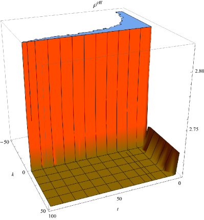
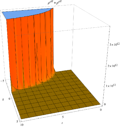
Figure 1: WEC plots for model 1 mentioned in Eq.(40) in extended $f(R,G,T)$ gravity. Left plot shows the behavior of $\rho^{eff}$ and right plot show the behavior of $\rho^{eff}+P^{eff}$ with respect to $t$ and $k$ for $\alpha=\beta=1$, respectively.

In this context, the plotted region is illustrated in the right diagram of Fig.2. We concluded that the violation of WEC may be avoided by making all of the parameters ($t,~{}\alpha,~{}k$) to be positive in $f(R,G,T)=R+R^{2}+\alpha{G^{n}}+\beta G\log[G]+\gamma T^{k}$ model.

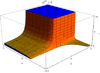
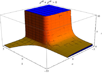
Figure 2: WEC plots for model 1 mentioned in Eq.(40) in extended $f(R,G,T)$ gravity. The left plot representing the regions where $\rho_{eff}>0$ while the right plot represents the regions where $\rho_{eff}+P_{eff}>0$ with respect to $\alpha$, $k$ and $t$, respectively. We see that the WECs is satisfied for the considered range of parameters.

• Validity of $\rho^{eff}>0$.
  

  We found that when $t\rightarrow 10$, the desire values of other parameter will get the values of $\alpha\rightarrow 9.92$ and $k\rightarrow-0.179$, while for $t\rightarrow 0.1$ we obtained $\alpha\rightarrow-1.399$ and $k\rightarrow 9.96$.
  

  For $\alpha\rightarrow 10$, the other parameter should be $t\rightarrow 0.227$ and $k\rightarrow 9.976$, while for $\alpha\rightarrow-10$ then $t\rightarrow 0.1$ and $k\rightarrow 7.078$.
  

  Similarly when $k\rightarrow 10$, the desire values of other parameter will get the values of $\alpha\rightarrow 3.88$ and $t\rightarrow 0.208$ while for $k\rightarrow-10$ we obtained $\alpha\rightarrow-1.673$ and $t\rightarrow 0.126$.
  

• Validity of $\rho^{eff}+P^{eff}>0$.
  

  We found that when $t\rightarrow 10$, the desire values of other parameter will get the values of $\alpha\rightarrow-1.39$ and $k\rightarrow 9.960$ while for $t\rightarrow 0.1$, we obtained $\alpha\rightarrow-0.896$ and $k\rightarrow 9.354$.
  

  For $\alpha\rightarrow 10$, the other parameter should be $t\rightarrow 0.170$ and $k\rightarrow 9.950$, while for $\alpha\rightarrow-10$ then $t\rightarrow 9.47$ and $k\rightarrow-0.05$.
  

  Similarly when $k\rightarrow 10$, the desire values of other parameter will get the values of $\alpha\rightarrow-4.99$ and $t\rightarrow 3.94$, while for $k\rightarrow-10$ we obtained $\alpha\rightarrow-1.673$ and $t\rightarrow 0.126$.
  

4.2 Model 2

Next, we look at a more realistic version of the $f(G)$ model [38], inspire from this, we suggest the following model as

$$f(R,G,T)=R+R^{2}+\alpha G^{n}\left(\beta G^{m}+1\right)+\gamma T^{k},$$ (43)

where $n$ is a positive constant and $\alpha,~{}\beta$, $k$, $m$ and $\gamma$ are the model parameters. This version might be beneficial for understanding future singularities in finite time [73]. Both the local assessment and the galactic limits agree with the conclusions of this hypothesis [74].
The effective energy density was calculated using Eq.(43) and found to be

$${\rho^{eff}} =\frac{1}{{\kappa^{2}\left({2R+1}\right)}}[12(m\alpha\beta{G^{-1+m+n}}+n\alpha{G^{-1+n}}(1+\beta{G^{m}}))$$

$${H^{2}}({H^{2}}-{H^{2}}(1+q))+\frac{1}{2}(-\alpha{G^{n}}\left({1+\beta{G^{m}}}\right)-R-{R^{2}}+R$$

$$\left({2R+1}\right)-\gamma{T^{k}})+\kappa^{2}\rho+k\gamma{T^{-1+k}}\left({p+\rho}\right)-12(mn\alpha\beta{G^{-2+m+n}}+m$$

$$(m+n-1)\alpha\beta{G^{-2+m+n}}+\left({n-1}\right)n\alpha{G^{-2+n}}\left({1+\beta{G^{m}}}\right)){H^{3}}G^{\prime}-6HR^{\prime}]\geq 0.$$ (44)

While the product of effective pressure and energy density is

$${\rho^{eff}}+{P^{eff}} =\frac{1}{{\left({{\kappa^{2}}{G^{3}}\left({1+2R}\right)T}\right)}}[4n\left({2-3n+{n^{2}}}\right)\alpha{G^{n}}{H^{2}}T{{G^{\prime}}^{2}}$$

$$+4({m^{3}}+3{m^{2}}\left({n-1}\right)+n(2-3n+{n^{2}})+m\left({2-6n+3{n^{2}}}\right))\alpha\beta{G^{m+n}}$$

$${H^{2}}T{{G^{\prime}}^{2}}-4\left({n-1}\right)n\alpha{G^{1+n}}{H^{2}}T(H\left({3+2q}\right)G^{\prime}-{G^{\prime\prime}})-4({m^{2}}+\left({n-1}\right)n$$

$$+m\left({2n-1}\right))\alpha\beta{G^{1+m+n}}{H^{2}}T(H\left({2q+3}\right)G^{\prime}-{G^{\prime\prime}})+{G^{3}}(p({\kappa^{2}}T+k\gamma{T^{k}})$$

$$+k\gamma{T^{k}}\rho+T({\kappa^{2}}\rho-2HR^{\prime}+2{R^{\prime\prime}}))]\geq 0.$$ (45)

Finding the exact analytical formula for the parameters for these two inequalities (4.2) and (4.2), are significantly more difficult. As a result, we’ll set some parameters identical to the specific values. For simplicity, we let $\alpha=1,\beta=1$ and plot $\rho^{\textrm{eff}}$ and $\rho^{\textrm{eff}}+P^{\textrm{eff}}$, as demonstrated in Fig.3. Here we consider $0<t<10$, $-5<k<5$ and $-5<\alpha<5$. WECs is also valid for the model (43) as can be seen in this diagram.

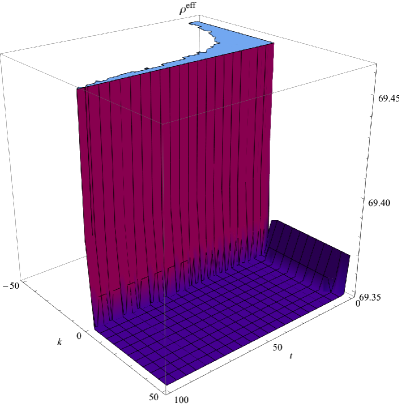
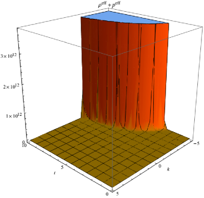
Figure 3: WEC plots for model 2 mentioned in Eq.(43) in extended $f(R,G,T)$ gravity. Left plot show the behavior of $\rho^{eff}$ and right plot show the behavior of $\rho^{eff}+P^{eff}$ with respect to $t$ and $k$ for $\alpha=\beta=1$, respectively.

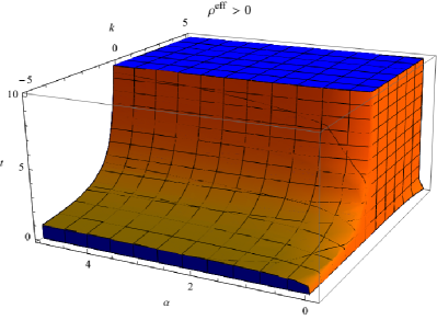
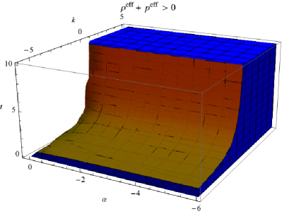
Figure 4: WECs plots for model 2 mentioned in Eq.(43) in extended $f(R,G,T)$ gravity. The left plot representing the regions where $\rho_{eff}>0$, while the right plot represents the regions where $\rho_{eff}+P_{eff}>0$ with respect to $\alpha$, $k$ and $t$, respectively. We see that the WECs is satisfied for the considered range of parameters.

• Validity of $\rho^{eff}>0$.
  

  We found that when $t\rightarrow 10$, the desire values of other parameter will get the values of $\alpha\rightarrow 9.936$ and $k\rightarrow-0.379$, while for $t\rightarrow 0.1$ we obtained $\alpha\rightarrow 1.080$ and $k\rightarrow 9.957$.
  

  For $\alpha\rightarrow 10$, the other parameters should be $t\rightarrow 0.227$ and $k\rightarrow 9.976$, while for $\alpha\rightarrow 0.769$ then $t\rightarrow 0.1$ and $k\rightarrow 10$.
  

  Similarly, when $k\rightarrow 10$, the desire values of other parameter will get the values of $\alpha\rightarrow 0.0388$ and $t\rightarrow 0.230$ while for $k\rightarrow-10$, we obtained $\alpha\rightarrow 10$ and $t\rightarrow 0.1$.
  

  Validity of $\rho^{eff}+P^{eff}>0$.
  

  We found that when $t\rightarrow 10$, the desire values of other parameter will get the values of $\alpha\rightarrow-9.94$ and $k\rightarrow 5.15$ while for $t\rightarrow 0.1$ we obtained $\alpha\rightarrow-4.75$ and $k\rightarrow-9.78$.
  

  For $\alpha\rightarrow 1.17$, the other parameters should be $t\rightarrow 1.17$ and $k\rightarrow 0.1$ while for $\alpha\rightarrow-10$ then $t\rightarrow 7.19$ and $k\rightarrow 9.34$.
  

  Similarly, when $k\rightarrow 10$, the desire values of other parameter will get the values of $\alpha\rightarrow-9.58$ and $t\rightarrow 9.99$ while for $k\rightarrow-10$, we obtained $\alpha\rightarrow 10$ and $t\rightarrow 0.1$.
  

4.3 Model 3

Some other plausible gravity $f(G)$ model would be fascinating to investigate [37], in this regard, we suggest the following model as

$$f(R,G,T)=R+R^{2}+\frac{{{a_{1}}{G^{n}}+{b_{1}}}}{{{a_{2}}{G^{n}}+{b_{2}}}}+\gamma T^{k},$$ (46)

Here, $a_{1},~{}b_{1},~{}a_{2},~{}b_{2}$, $k$, $\gamma$ and $n$ are random constants with $n>0$. This model could be beneficial for studying future singularities in early time and late time cosmic acceleration. The effective energy density in this regard

$${\rho^{eff}} =\frac{1}{{{\kappa^{2}}\left({2R+1}\right)}}[12(-{a_{2}}n{G^{-1+n}}\left({b_{1}+a_{1}{G^{n}}}\right)$$

$${\left({b_{2}+{a_{2}}{G^{n}}}\right)^{-2}}+a_{1}n{\left({b_{2}+a_{2}{G^{n}}}\right)^{-1}}{G^{-1+n}}){H^{2}}\left({{H^{2}}-{H^{2}}\left({1+q}\right)}\right)$$

$$+\frac{1}{2}(-(b_{1}+a_{1}{G^{n}}){\left({b_{2}+a_{2}{G^{n}}}\right)^{-1}}-R-{R^{2}}+R\left({2R+1}\right)-\gamma{T^{k}})$$

$$+{\kappa^{2}}\rho+k\gamma{T^{-1+k}}\left({p+\rho}\right)-12(2a_{2}^{2}{n^{2}}{G^{-2+2n}}\left({b_{1}+a_{1}{G^{n}}}\right){\left({b_{2}+a_{2}{G^{n}}}\right)^{-3}}$$

$$-2a_{1}a_{2}{n^{2}}{\left({b_{2}+a_{2}{G^{n}}}\right)^{-2}}{G^{-2+2n}}-a_{2}\left({n-1}\right)n{G^{-2+n}}{\left({b_{2}+a_{2}{G^{n}}}\right)^{-2}}$$

$$\left({b_{1}+a_{1}{G^{n}}}\right)+a_{1}\left({n-1}\right){\left({b_{2}+a_{2}{G^{n}}}\right)^{-1}}n{G^{-2+n}}){H^{3}}G^{\prime}-6HR^{\prime}]\geq 0.$$ (47)

Where the effective energy density and pressure are combined to form

$${\rho^{eff}}+{P^{eff}} =\frac{1}{{\left\{{{\kappa^{2}}{G^{3}}{{\left({b_{2}+a_{2}{G^{n}}}\right)}^{4}}\left({1+2R}\right)T}\right\}}}[4b_{2}^{2}\left({-a_{2}b_{1}+a_{1}b_{2}}\right)$$

$$n\left({{n^{2}}-3n+2}\right){G^{n}}{H^{2}}T{{G^{\prime}}^{2}}+16a_{2}b_{2}\left({a_{2}b_{1}-a_{1}b_{2}}\right)n\left({{n^{2}}-1}\right){G^{2n}}{H^{2}}T{{G^{\prime}}^{2}}$$

$$-4a_{2}^{2}\left({a_{2}b_{1}-a_{1}b_{2}}\right)n\left({{n^{2}}+3n+2}\right){G^{3n}}{H^{2}}T{{G^{\prime}}^{2}}+4b_{2}^{2}\left({a_{2}b_{1}-a_{1}b_{2}}\right)$$

$$\left({n-1}\right)n{G^{1+n}}{H^{2}}T(H\left({3+2q}\right)G^{\prime}-{G^{\prime\prime}})-8a_{2}b_{2}\left({a_{2}b_{1}-a_{1}b_{2}}\right)n{G^{1+2n}}{H^{2}}T$$

$$\left({H\left({3+2q}\right)G^{\prime}-{G^{\prime\prime}}}\right)-4a_{2}^{2}\left({a_{2}b_{1}-a_{1}b_{2}}\right)n\left({1+n}\right){G^{1+3n}}{H^{2}}T(H\left({3+2q}\right)G^{\prime}$$

$$-{G^{\prime\prime}})+b_{2}^{4}{G^{3}}\left({p\left({{\kappa^{2}}T+k\gamma{T^{k}}}\right)+k\gamma{T^{k}}\rho+T\left({{\kappa^{2}}\rho-2HR^{\prime}+2{R^{\prime\prime}}}\right)}\right)+4a_{2}b_{2}^{3}$$

$${G^{3+n}}(p\left({{\kappa^{2}}T+k\gamma{T^{k}}}\right)+k\gamma{T^{k}}\rho+T\left({{\kappa^{2}}\rho-2HR^{\prime}+2{R^{\prime\prime}}}\right))+6a_{2}^{2}b_{2}^{2}{G^{3+2n}}$$

$$\left({p\left({{\kappa^{2}}T+k\gamma{T^{k}}}\right)+k\gamma{T^{k}}\rho+T\left({{\kappa^{2}}\rho-2HR^{\prime}+2{R^{\prime\prime}}}\right)}\right)+4a_{2}^{3}b_{2}{G^{3+3n}}$$

$$(p\left({{\kappa^{2}}T+k\gamma{T^{k}}}\right)+k\gamma{T^{k}}\rho+T\left({{\kappa^{2}}\rho-2HR^{\prime}+2{R^{\prime\prime}}}\right))+a_{2}^{4}{G^{3+4n}}(p$$

$$\left({{\kappa^{2}}T+k\gamma{T^{k}}}\right)+k\gamma{T^{k}}\rho+T\left({{\kappa^{2}}\rho-2HR^{\prime}+2{R^{\prime\prime}}}\right))]\geq 0.$$ (48)

This model having variables, i.e., $a_{1},~{}a_{2},~{}b_{1},~{}b_{2},~{}m$, so we’ll assign few specific values to some of these parameters to constraint them with a specific range. For the sake of simplicity, we’ll set $b_{1}=-1,b_{2}=1$. Here we consider $0<t<10$, $-5<k<5$ and $-5<\alpha<5$. Other attributes are:

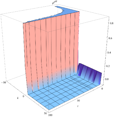
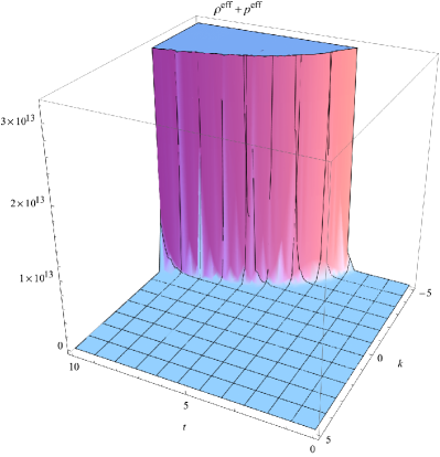
Figure 5: WEC plots for model 3 mentioned in Eq.(46) in extended $f(R,G,T)$ gravity. Left plot show the behavior of $\rho^{eff}$ and right plot show the behavior of $\rho^{eff}+P^{eff}$ with respect to $t$ and $k$ for $\alpha=\beta=1$, respectively.

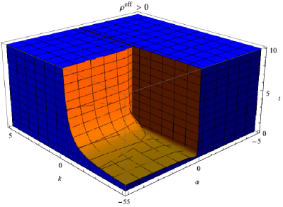
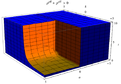
Figure 6: WECs plots for model 3 mentioned in Eq.(46) in extended $f(R,G,T)$ gravity. The left plot representing the regions where $\rho_{eff}>0$ while the right plot represents the regions where $\rho_{eff}+P_{eff}>0$ with respect to $\alpha$, $k$ and $t$, respectively. We see that the WECs is satisfied for the considered range of parameters.

• Validity of $\rho^{eff}>0$.
  

  We found that when $t\rightarrow 10$, the desire values of other parameter will get the values of $\alpha\rightarrow 3.077$ and $k\rightarrow 9.894$, while for $t\rightarrow 0.1$ we obtained $\alpha\rightarrow-9.093$ and $k\rightarrow-3.349$.
  

  For $\alpha\rightarrow 10$, the other parameter should be $t\rightarrow 9.942$ and $k\rightarrow 8.316$ while for $\alpha\rightarrow-10$ then $t\rightarrow 0.137$ and $k\rightarrow-9.99$.
  

  Similarly, when $k\rightarrow 10$, the desire values of other parameter will get the values of $\alpha\rightarrow 2.151$ and $t\rightarrow 9.64$ while for $k\rightarrow-10$ we obtained $\alpha\rightarrow-7.29$ and $t\rightarrow 0.987$.
  

• Validity of $\rho^{eff}+P^{eff}>0$.
  

  We found that when $t\rightarrow 10$, the desire values of other parameter will get the values of $\alpha\rightarrow-3.077$ and $k\rightarrow 8.316$ while for $t\rightarrow 0.1$ we obtained $\alpha\rightarrow-6.01$ and $k\rightarrow-9.768$.
  

  For $\alpha\rightarrow 1.17$, the other parameter should be $t\rightarrow 9.942$ and $k\rightarrow 8.316$ while for $\alpha\rightarrow-10$ then $t\rightarrow 0.137$ and $k\rightarrow-9.99$.
  

  Similarly, when $k\rightarrow 10$, the desire values of other parameter will get the values of $\alpha\rightarrow 2.15$ and $t\rightarrow 9.64$ while for $k\rightarrow-10$. We obtained $\alpha\rightarrow-7.29$ and $t\rightarrow 0.98$.
  

5 Stability of Models

It is crucial to make an argument for the stability of the suggested models in the $f(R,G,T)$ gravity theory here. This universe can be thought of as a thermodynamical system given that it is made up entirely of perfect fluid. This goal is accomplished by introducing an arbitrary function (the quantity of sound speed ($c_{s}^{2}$)) to describe the system made up of the ideal fluid. This arbitrary function can be expressed in terms of the universe’s effective energy density ($\rho_{eff}$) and effective pressure ($P_{eff}$ ) as follows:

$$c_{s}^{2}=\frac{dP_{eff}}{d\rho_{eff}}.$$

It is known that the value of the aforementioned function is greater than zero for a thermodynamic system. In light of this, stability conditions can be verified when $c_{s}^{2}>0$. Using adiabatic and non-adiabatic methods, a thermodynamic system can be explained perturbatively. Effective energy density, effective pressure, and universe entropy are three potential disturbance quantities in this situation. The stability of our models can plotted in Fig. 7.

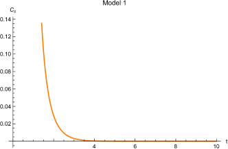
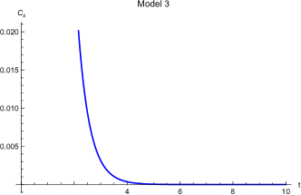
Figure 7: Stability of Models

6 Summary

We investigated the impact of enhanced extended theory of gravity models on the occurrence of actual cosmological perfect fluid configurations. The study of ECs are inextricably linked to a pragmatic representation of WH solutions [75, 76, 77, 78, 79, 80]. Inspection of plausible and quite well models is an enticing goal for avoiding the utilization of unusual matter content at the WH throat. We looked at the behaviour of the FLRW metric when it was full with an perfect fluid. The field equations $f(R,G,T)$ turn out to be extremely nonlinear, and Even without any fundamentally coherent principles, they can’t be solved. We calculated the general energy inequalities relationship using $f(R,G,T)$ field equations. Three separate customized extended theory of gravity simulations were examined, i.e., $f(R,G,T)=R+R^{2}+\alpha{G^{n}}+\beta G\log[G]+\gamma T^{k},~{}f(R,G,T)=R+R^{2}+\alpha G^{n}\left(\beta G^{m}+1\right)+\gamma T^{k}$ and $f(R,G,T)=R+R^{2}+\frac{{{a_{1}}{G^{n}}+{b_{1}}}}{{{a_{2}}{G^{n}}+{b_{2}}}}+\gamma T^{k}$. We examined the behaviour of ECs using all of the customized extended models discussed over. Then, with the several possible $f(R,G,T)$ models, the most likely measured results of the parameters; Hubble, deceleration, jerk, and snap are employed. The areas where NEC and WEC maintain under different $f(R,G,T)$ gravity values were displayed. Here, we consider $0<t<10$, $-5<k<5$ and $-5<\alpha<5$. These following are several of the graphical features that demonstrate some of the results:
Bounds on Model 1:

• For time, $0<t<1$, $\rho>0$ for all $k$, along with $\alpha>-1.7$.

• For parameter $k$, $4<k<5$, $\rho>0$ for all $\alpha$, along with a very small $t$.

• Furthermore, $\rho>0$ for $t>0$, along with $k<0$ and $\alpha>-1.7$.

Bounds on Model 2:

• For small value of (e.g., $0<t<1$), the density, $\rho>0$ for any value of $k$, along with positive value of $\alpha>0$.

• For $t>1$, the validity of $\rho>0$ required both $\alpha>0$ with $k>0$.

• For small value of (e.g., $0<t<1$), the density, $\rho+P>0$ for any value of $k$, along with positive value of $\alpha<0$.

• For $t>1$, the validity of $\rho+P>0$ required both $\alpha<0$ with $k>0$.

Bounds on Model 3:

• For $0<t<1$, the validity of WEC required the parameter $k$ and $\alpha$ to be any value in given range.

• For $t>1$, WEC bounds the parameters $\alpha<0$, along with any value of $k$.

• Similarly, for $t>1$, WEC also restrict the parameters $\alpha>0$, along with any value of $k>0$.

The suggested models’ solutions found in this research will be useful for creating a physical and realistic model that accounts for the universe’s acceleration. When compared to the discussion of pure gravity, theoretical study may then produce some qualitative outcomes. It will be used somewhere else.
It is important to look into the possibility of our models’ solutions for various cosmological phases. Because they exist in a FLRW background that reflects all potential cosmic evolutions, including the dark energy period, matter dominant, or radiation dominant eras, these solutions are especially significant.

References

- [1] Davide Pietrobon, Amedeo Balbi, and Domenico Marinucci. Integrated sachs-wolfe effect from the cross correlation of wmap 3 year and the nrao vla sky survey data: New results and constraints on dark energy. Physical Review D, 74(4):043524, 2006.
- [2] Tommaso Giannantonio, Robert G Crittenden, Robert C Nichol, Ryan Scranton, Gordon T Richards, Adam D Myers, Robert J Brunner, Alexander G Gray, Andrew J Connolly, and Donald P Schneider. High redshift detection of the integrated sachs-wolfe effect. Physical Review D, 74(6):063520, 2006.
- [3] Adam G Riess, Louis-Gregory Strolger, Stefano Casertano, Henry C Ferguson, Bahram Mobasher, Ben Gold, Peter J Challis, Alexei V Filippenko, Saurabh Jha, Weidong Li, et al. New hubble space telescope discoveries of type ia supernovae at z= 1: narrowing constraints on the early behavior of dark energy. The Astrophysical Journal, 659(1):98, 2007.
- [4] J Delabrouille, P De Bernardis, FR Bouchet, A Achúcarro, PAR Ade, R Allison, F Arroja, E Artal, M Ashdown, C Baccigalupi, et al. Exploring cosmic origins with core: Survey requirements and mission design. Journal of Cosmology and Astroparticle Physics, 2018(04):014, 2018.
- [5] Peter AR Ade, N Aghanim, M Arnaud, Mark Ashdown, J Aumont, C Baccigalupi, AJ Banday, RB Barreiro, JG Bartlett, N Bartolo, et al. Planck 2015 results-xiii. cosmological parameters. Astronomy & Astrophysics, 594:A13, 2016.
- [6] PAR Ade, N Aghanim, M Arnaud, F Arroja, Mark Ashdown, J Aumont, C Baccigalupi, M Ballardini, AJ Banday, RB Barreiro, et al. Planck 2015 results-xx. constraints on inflation. Astronomy & Astrophysics, 594:A20, 2016.
- [7] Peter AR Ade, RW Aikin, D Barkats, SJ Benton, CA Bischoff, JJ Bock, JA Brevik, I Buder, E Bullock, CD Dowell, et al. Detection of b-mode polarization at degree angular scales by bicep2. Physical Review Letters, 112(24):241101, 2014.
- [8] Planck Collaborations, PAR Ade, N Aghanim, Z Ahmed, RW Aikin, KD Alexander, M Arnaud, J Aumont, C Baccigalupi, AJ Banday, et al. A joint analysis of bicep2/keck array and planck data. arXiv preprint arXiv:1502.00612, 2015.
- [9] Keck Array, BICEP Collaborations, PAR Ade, Z Ahmed, RW Aikin, KD Alexander, D Barkats, SJ Benton, CA Bischoff, JJ Bock, et al. Bicep2. arXiv preprint arXiv:1510.09217, 2015.
- [10] Eiichiro Komatsu, J Dunkley, MR Nolta, CL Bennett, B Gold, G Hinshaw, N Jarosik, D Larson, M Limon, L Page, et al. Five-year wilkinson microwave anisotropy probe* observations: cosmological interpretation. The Astrophysical Journal Supplement Series, 180(2):330, 2009.
- [11] Gary Hinshaw, D Larson, Eiichiro Komatsu, David N Spergel, CLaa Bennett, Joanna Dunkley, MR Nolta, M Halpern, RS Hill, N Odegard, et al. Nine-year wilkinson microwave anisotropy probe (wmap) observations: cosmological parameter results. The Astrophysical Journal Supplement Series, 208(2):19, 2013.
- [12] Austin Joyce, Bhuvnesh Jain, Justin Khoury, and Mark Trodden. Beyond the cosmological standard model. Physics Reports, 568:1–98, 2015.
- [13] Salvatore Capozziello and Mariafelicia De Laurentis. Extended theories of gravity. Physics Reports, 509(4-5):167–321, 2011.
- [14] Kazuharu Bamba, Salvatore Capozziello, Shinichi Nojiri, and Sergei D Odintsov. Dark energy cosmology: the equivalent description via different theoretical models and cosmography tests. Astrophysics and Space Science, 342(1):155–228, 2012.
- [15] Kazuya Koyama. Cosmological tests of modified gravity. Reports on Progress in Physics, 79(4):046902, 2016.
- [16] De la Cruz-Dombriz, Diego Sáez-Gómez, et al. Black holes, cosmological solutions, future singularities, and their thermodynamical properties in modified gravity theories. Entropy, 14(9):1717–1770, 2012.
- [17] Kazuharu Bamba, Shin’ichi Nojiri, and Sergei D Odintsov. Modified gravity: walk through accelerating cosmology. arXiv preprint arXiv:1302.4831, 2013.
- [18] Kazuharu Bamba and Sergei D Odintsov. Universe acceleration in modified gravities: and cases. arXiv preprint arXiv:1402.7114, 2014.
- [19] Z Yousaf, Kazuharu Bamba, et al. Influence of modification of gravity on the dynamics of radiating spherical fluids. Physical Review D, 93(6):064059, 2016.
- [20] Z Yousaf, Kazuharu Bamba, and M Zaeem-ul-Haq Bhatti. Causes of irregular energy density in gravity. Physical Review D, 93(12):124048, 2016.
- [21] SI Nojiri and SD Odintsov. econf c0602061, 06 (2006). Int. J. Geom. Meth. Mod. Phys, 4(115):16, 2007.
- [22] Shin’ichi Nojiri and Sergei D Odintsov. Can -gravity be a viable model: the universal unification scenario for inflation, dark energy and dark matter. arXiv preprint arXiv:0801.4843, 2008.
- [23] Shin’ichi Nojiri and Sergei D Odintsov. Dark energy, inflation and dark matter from modified gravity. arXiv preprint arXiv:0807.0685, 2008.
- [24] SH Hendi, B Eslam Panah, and C Corda. Asymptotically lifshitz black hole solutions in gravity. Canadian Journal of Physics, 92(1):76–81, 2014.
- [25] S Capozziello, M De Laurentis, I De Martino, M Formisano, and SD Odintsov. Jeans analysis of self-gravitating systems in gravity. Physical Review D, 85(4):044022, 2012.
- [26] Shinichi Nojiri and Sergei D Odintsov. Modified gravity with negative and positive powers of curvature: Unification of inflation and cosmic acceleration. physical Review D, 68(12):123512, 2003.
- [27] Z Yousaf. Stellar filaments with minkowskian core in the einstein- gravity. The European Physical Journal Plus, 132(6):1–14, 2017.
- [28] M Sharif and Z Yousaf. Role of adiabatic index on the evolution of spherical gravitational collapse in palatini gravity. Astrophysics and Space Science, 355(2):317–331, 2015.
- [29] Z Yousaf and M Bhatti. Cavity evolution and instability constraints of relativistic interiors. The European Physical Journal C, 76(5):1–15, 2016.
- [30] Sergei D Odintsov and Diego Sáez-Gómez. gravity phenomenology and cdm universe. Physics Letters B, 725(4-5):437–444, 2013.
- [31] Shin’ichi Nojiri and Sergei D Odintsov. Modified gauss–bonnet theory as gravitational alternative for dark energy. Physics Letters B, 631(1-2):1–6, 2005.
- [32] Guido Cognola, Emilio Elizalde, Shinichi Nojiri, Sergei D Odintsov, and Sergio Zerbini. String-inspired gauss-bonnet gravity reconstructed from the universe expansion history and yielding the transition from matter dominance to dark energy. Physical Review D, 75(8):086002, 2007.
- [33] Seyed H Hendi, Ahmad Sheykhi, and Mehdi H Dehghani. Thermodynamics of higher dimensional topological charged ads black branes in dilaton gravity. The European Physical Journal C, 70(3):703–712, 2010.
- [34] Ben M Leith and Ishwaree P Neupane. Gauss-bonnet cosmologies: crossing the phantom divide and the transition from matter dominance to dark energy. Journal of Cosmology and Astroparticle Physics, 2007(05):019, 2007.
- [35] Antonio De Felice and Shinji Tsujikawa. Construction of cosmologically viable gravity models. Physics Letters B, 675(1):1–8, 2009.
- [36] Shinichi Nojiri and Sergei D Odintsov. Unified cosmic history in modified gravity: from theory to lorentz non-invariant models. Physics Reports, 505(2-4):59–144, 2011.
- [37] Shin’ichi Nojiri, Sergei D Odintsov, and Petr V Tretyakov. From inflation to dark energy in the non-minimal modified gravity. Progress of Theoretical Physics Supplement, 172:81–89, 2008.
- [38] Kazuharu Bamba, Sergei D Odintsov, Lorenzo Sebastiani, and Sergio Zerbini. Finite-time future singularities in modified gauss–bonnet and gravity and singularity avoidance. The European Physical Journal C, 67(1):295–310, 2010.
- [39] Antonio De Felice and Shinji Tsujikawa. Solar system constraints on gravity models. Physical Review D, 80(6):063516, 2009.
- [40] JH Kung. gravity as + back reaction. Physical Review D, 52(12):6922, 1995.
- [41] JH Kung. Strong energy condition in gravity. Physical Review D, 53(6):3017, 1996.
- [42] SE Perez Bergliaffa. Constraining theories with the energy conditions. Physics Letters B, 642(4):311–314, 2006.
- [43] Sh Nojiri, SD Odintsov, and VK3683913 Oikonomou. Modified gravity theories on a nutshell: inflation, bounce and late-time evolution. Physics Reports, 692:1–104, 2017.
- [44] Stephen W Hawking and George Francis Rayner Ellis. The large scale structure of space-time, volume 1. Cambridge university press, 1973.
- [45] Robert M Wald. General relativity. University of Chicago press, 2010.
- [46] Sean M Carroll. An introduction to general relativity: spacetime and geometry. Addison Wesley, 101:102, 2004.
- [47] M Ilyas. Energy conditions in non-local gravity. International Journal of Geometric Methods in Modern Physics, 16(10):1950149, 2019.
- [48] M Ilyas, Z Yousaf, and MZ Bhatti. Bounds on higher derivative models from energy conditions. Modern Physics Letters A, 34(11):1950082, 2019.
- [49] Z Yousaf, M Sharif, M Ilyas, and M Zaeem-ul Haq Bhatti. Energy conditions in higher derivative gravity. International Journal of Geometric Methods in Modern Physics, 15(09):1850146, 2018.
- [50] Kazuharu Bamba, M Ilyas, MZ Bhatti, and Z Yousaf. Energy conditions in modified gravity. General Relativity and Gravitation, 49(8):1–17, 2017.
- [51] Janilo Santos and JS Alcaniz. Energy conditions and segre classification of phantom fields. Physics Letters B, 619(1-2):11–16, 2005.
- [52] Jessica Santiago, Sebastian Schuster, and Matt Visser. Generic warp drives violate the null energy condition. Physical Review D, 105(6):064038, 2022.
- [53] Matt Visser. General relativistic energy conditions: The hubble expansion in the epoch of galaxy formation. Physical Review D, 56(12):7578, 1997.
- [54] J Santos, JS Alcaniz, and MJ Rebouças. Energy conditions and supernovae observations. Physical Review D, 74(6):067301, 2006.
- [55] J Santos, JS Alcaniz, N Pires, and Marcelo J Reboucas. Energy conditions and cosmic acceleration. Physical Review D, 75(8):083523, 2007.
- [56] AA Sen and Robert J Scherrer. The weak energy condition and the expansion history of the universe. Physics Letters B, 659(3):457–461, 2008.
- [57] J Santos, JS Alcaniz, MJ Reboucas, and N Pires. Lookback time bounds from energy conditions. Physical Review D, 76(4):043519, 2007.
- [58] Yungui Gong, Anzhong Wang, Qiang Wu, and Yuan-Zhong Zhang. Direct evidence of acceleration from a distance modulus–redshift graph. Journal of Cosmology and Astroparticle Physics, 2007(08):018, 2007.
- [59] Yungui Gong and Anzhong Wang. Energy conditions and current acceleration of the universe. Physics Letters B, 652(2-3):63–68, 2007.
- [60] J Santos, JS Alcaniz, MJ Reboucas, and FC Carvalho. Energy conditions in gravity. Physical Review D, 76(8):083513, 2007.
- [61] JANILO SANTOS, MARCELO J REBOUÇAS, and JAILSON S ALCANIZ. Energy conditions constraints on a class of -gravity. International Journal of Modern Physics D, 19(08n10):1315–1321, 2010.
- [62] K Atazadeh, A Khaleghi, HR Sepangi, and Y Tavakoli. Energy conditions in gravity and brans–dicke theories. International Journal of Modern Physics D, 18(07):1101–1111, 2009.
- [63] Orfeu Bertolami and Miguel Carvalho Sequeira. Energy conditions and stability in theories of gravity with nonminimal coupling to matter. Physical Review D, 79(10):104010, 2009.
- [64] Nadiezhda Montelongo Garcia, Tiberiu Harko, Francisco SN Lobo, and José P Mimoso. Energy conditions in modified gauss-bonnet gravity. Physical Review D, 83(10):104032, 2011.
- [65] Nadiezhda M García, Francisco SN Lobo, José P Mimoso, and Tiberiu Harko. f (g) modified gravity and the energy conditions. In Journal of Physics: Conference Series, volume 314, page 012056. IOP Publishing, 2011.
- [66] J Sadeghi, A Banijamali, and H Vaez. Constraining gravity models using energy conditions. International Journal of Theoretical Physics, 51(9):2888–2899, 2012.
- [67] Snehasish Bhattacharjee. Energy conditions in gravity. arXiv preprint arXiv:2103.08444, 2021.
- [68] M Ilyas. Charged compact stars in gravity. The European Physical Journal C, 78(9):1–12, 2018.
- [69] M Ilyas. Compact stars in gravity. International Journal of Modern Physics A, 36(24):2150165, 2021.
- [70] M Sharif, S Rani, and R Myrzakulov. Analysis of gravity models through energy conditions. The European Physical Journal Plus, 128(10):1–11, 2013.
- [71] Hans-Jürgen Schmidt. Gauss-bonnet lagrangian and cosmological exact solutions. Physical Review D, 83(8):083513, 2011.
- [72] MR Setare and N Mohammadipour. Cosmography in modified gravity. arXiv preprint arXiv:1206.0245, 2012.
- [73] Shinichi Nojiri and Sergei D Odintsov. Future evolution and finite-time singularities in gravity unifying inflation and cosmic acceleration. Physical Review D, 78(4):046006, 2008.
- [74] Shinichi Nojiri and Sergei D Odintsov. Unified cosmic history in modified gravity: from theory to lorentz non-invariant models. Physics Reports, 505(2-4):59–144, 2011.
- [75] M Ilyas, WU Rahman, S Ullah, F Khan, H Ullah, and R Khan. Wormhole solutions through hyperbolic model in gravity. International Journal of Modern Physics D, 31(05):2250034, 2022.
- [76] M Ilyas and AR Athar. Some specific wormhole solutions in gravity. Physica Scripta, 97(4):045003, 2022.
- [77] Z Yousaf, A Ikram, M Ilyas, and MZ Bhatti. Existence of dynamical wormholes in gravity. Canadian Journal of Physics, 98(5):474–483, 2020.
- [78] MZ Bhatti, Z Yousaf, and M Ilyas. Existence of wormhole solutions and energy conditions in gravity. Journal of Astrophysics and Astronomy, 39(6):1–11, 2018.
- [79] Z Yousaf, M Ilyas, and MZ Bhatti. Influence of modification of gravity on spherical wormhole models. Modern Physics Letters A, 32(30):1750163, 2017.
- [80] Z Yousaf, M Ilyas, and M Zaeem-ul Haq Bhatti. Static spherical wormhole models in gravity. The European Physical Journal Plus, 132(6):1–12, 2017.