A Proof of the Tree of Shapes in $n$-D

Abstract

In this paper, we prove that the self-dual morphological hierarchical structure computed on a $n$-D gray-level well-composed image $u$ by the algorithm of Géraud et al. [geraud.2013.ismm] is exactly the mathematical structure defined to be the tree of shape of $u$ in Najman et al [najman.2013.ismm]. We recall that this algorithm is in quasi-linear time and thus considered to be optimal. The tree of shapes leads to many applications in mathematical morphology and in image processing like grain filtering, shapings, image segmentation, and so on.

I Introduction

The material presented here is a formal proof that the hierarchical structure provided by the main algorithm in [geraud.2013.ismm] is the tree of shapes presented in [najman.2013.ismm]. This proof is $n$-dimensional.

II Mathematical background

In the following, we consider a $n$-D digital image $u$ as a function defined on a regular cubical $n$-D grid and having integral values (even if we can generalize our case to any totally ordered set); in brief, we have then $u:\mathbb{Z}^{n}\rightarrow\mathbb{Z}$.

Practically a digital image is defined on a finite domain, usually an hyper-rectangle $\{\,(z_{1},\ldots,z_{n})\,|\,\forall i,\,0\leq z_{i}<N_{i}\,\}$, so the number of points is $N=\prod_{i=1}^{n}N_{i}$, and the space of values is restricted to $\llbracket\,0,\,2^{Q}-1\,\rrbracket$, where $Q$ is the quantization. We are interested in computing the tree of shapes of such images.

For generality purpose, we give below some definitions related to a function $f$ defined upon a discrete set $X$ and taking values in a finite set $Y$; we have $f:X\rightarrow Y$. With $X$ having some discrete topology, for any subset $E\subset X$, we denote by $\mathcal{CC}(E)$ the set of connected components of $E$. Given $x\in X$, we denote by $\mathcal{CC}(E,x)$ the connected component of $E$ containing $x$ if $x\in E$; otherwise, we set $\mathcal{CC}(E,x):=\emptyset$.

II-A The tree of shapes in $\mathbb{Z}^{n}$

Let us now consider $X$ as being defined on the regular cubical $n$-D grid $\mathbb{Z}^{n}$ or on one of its subdivisions like $\frac{1}{s}\mathbb{Z}^{n}$ with $s\in\mathbb{N}^{*}$. Furthermore, $X$ is unicoherent in the sense that it is connected and for any two subsets $A,B$ ox $X$, the set $A\cap B$ is connected.

As usual in discrete topology, to properly deal with subsets of $\mathbb{Z}^{n}$ and with their complementary in $\mathbb{Z}^{n}$, we consider the dual connectivities ${c_{2n}}$ and ${c_{3^{n}-1}}$.

The extension from set to gray-level images is done using what are called threshold sets. For any $\lambda\in\mathbb{R}$, the subsets of $X$:

$$[\,u<\lambda\,] \,:=\,\{\,x\in X\;|\;u(x)<\lambda\,\},$$

$$\text{and~{}}[\,u\geq\lambda\,] \,:=\,\{\,x\in X\;|\;u(x)\geq\lambda\,\}$$

are respectively called the strict lower threshold set and large upper threshold set of the function $f$ relatively to (the threshold) $\lambda$. The sets $[\,u<\lambda\,]$ and $[\,u\geq\lambda\,]$ can be understood as binary images.

From these two families of threshold sets, we can deduce two sets, $\mathcal{T}_{<}(u)$ and $\mathcal{T}_{\geq}(u)$, composed of the connected components of respectively lower and upper cuts of $u$:

$$\mathcal{T}_{<}(u) \,=\,\{\,\Gamma\in\mathcal{CC}_{c_{2n}}([\,u<\lambda\,])\,\}_{\lambda},$$

$$\mathcal{T}_{\geq}(u) \,=\,\{\,\Gamma\in\mathcal{CC}_{c_{3^{n}-1}}([\,u\geq\lambda\,])\,\}_{\lambda}.$$

The elements of $\mathcal{T}_{<}(u)$ and $\mathcal{T}_{\geq}(u)$ respectively give rise to two dual trees: the min-tree and the max-tree of $u$.

Let us recall what we call a shape but before let us reintroduce some mathematical basics for mathematical morphology. The saturation operator fills in the cavities of subsets of a topological space $\Omega$ this way for any $\Gamma\subseteq\Omega$:

$$\mathrm{Sat}(\Gamma)=\Omega\setminus\mathcal{CC}(\Omega\setminus\Gamma,p_{\infty}).$$

In discrete topology, we obtain then for any $\Gamma\subseteq\mathbb{Z}^{n}$:

$$\mathrm{Sat}_{c_{3^{n}-1}}(\Gamma) \,:=\,\mathbb{Z}^{n}\setminus\mathcal{CC}_{c_{3^{n}-1}}(\mathbb{Z}^{n}\setminus\Gamma),$$

$$\mathrm{Sat}_{c_{2n}}(\Gamma) \,:=\,\mathbb{Z}^{n}\setminus\mathcal{CC}_{c_{2n}}(\mathbb{Z}^{n}\setminus\Gamma).$$

Based on these trees, we can define what we call the sets of shapes:

$$\mathcal{S}_{<}(u) \,:=\,\{\,\mathrm{Sat}_{c_{3^{n}-1}}(\Gamma);\;\Gamma\in\mathcal{T}_{<}(u)\,\}$$

$$\mathcal{S}_{\geq}(u) \,:=\,\{\,\mathrm{Sat}_{c_{2n}}(\Gamma);\;\Gamma\in\mathcal{T}_{\geq}(u)\,\}$$

$\mathcal{S}_{<}(u)$ is the set of lower shapes of $u$, $\mathcal{S}_{\geq}(u)$ is the set of upper shapes of $u$. They correspond to the sets of elements of the min- and max-trees when we have filled in their cavities using the saturation operator.

For a given subset $\Gamma\subseteq\Omega$, and for a arbitrarily chosen element $p_{\infty}\in\Omega$, then we call cavity each connected component of $\Omega\setminus\Gamma$ and which does not contain $p_{\infty}$. The connected component of $\Omega\setminus\Gamma$ containing $p_{\infty}$ is called the exterior of $\Gamma$ and can be empty.

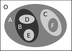
(a) Image $u$

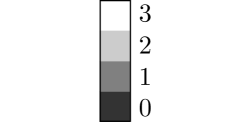
(b) Gray scale

(c) Level lines of $u$

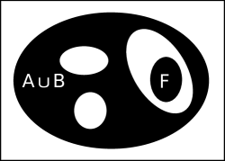
(d) ${[\,u<2\,]}$

(e) ${[\,u\geq 1\,]}$

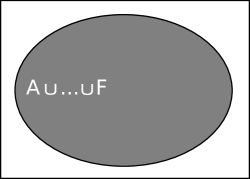
(f) A shape from (d)

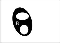
(g) ${[\,u<1\,]}$

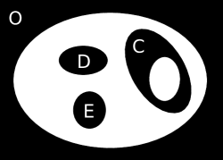
(h) ${[\,u\geq 2\,]}$

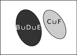
(i) Two shapes resp.       from (g) and (h)

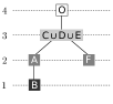
(j) Min-tree $\mathcal{T}_{<}(u)$

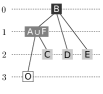
(k) Max-tree $\mathcal{T}_{\geq}(u)$

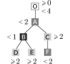
(l) Tree of shapes $\mathfrak{S}(u)$

Figure 1: Morphological trees.

The set of all shapes:

$$\mathfrak{S}(u)\,=\,\mathcal{S}_{<}(u)\,\cup\,\mathcal{S}_{\geq}(u)$$ (1)

forms a tree, the so-called tree of shapes of $u$ [monasse.2000.itip]. Indeed, for any pair of shapes $\Gamma$ and $\Gamma^{\prime}$ in $\mathfrak{S}$, we have $\Gamma\subset\Gamma^{\prime}\mbox{~{}~{}or~{}~{}}\Gamma^{\prime}\subset\Gamma\mbox{~{}~{}or~{}~{}}\Gamma\cap\Gamma^{\prime}=\emptyset$.

Actually, the shapes are the cavities of the elements of $\mathcal{T}_{<}$ and $\mathcal{T}_{\geq}$. For instance, if we consider a lower component $\Gamma\in[\,f<\lambda\,]$ and a cavity $H$ of $\Gamma$, this cavity is an upper shape, i.e., $H\in\mathcal{S}_{\geq}$. Furthermore, in a discrete setting, $H$ is obtained after having filled the cavities of a component of $[\,f\geq\lambda\,]$.

Figure 1 depicts on a sample image the three components trees ($\mathcal{T}_{<}$, $\mathcal{T}_{\geq}$, and $\mathfrak{S}$). Just note that the Equations so far rely on the pair of dual connectivities, ${c_{2n}}$ and ${c_{3^{n}-1}}$, so discrete topological problems are avoided, and, in addition, we are forced to consider two kind of cuts: strict ones for ${c_{2n}}$ and large ones for ${c_{3^{n}-1}}$.

II-B Cellular complex and Khalimsky grid

Let us recall the definitions relative to $n$-D Khalimsky grids [khalimsky1990computer, mazo.2012.jmiv.a]. From the sets $\mathbb{H}^{1}_{0}=\,\{\{a\};a\in\mathbb{Z}\}\,$ and $\mathbb{H}^{1}_{1}\,=\,\{\{a,a+1\};a\in\mathbb{Z}\}$, we can define $\mathbb{H}^{1}\,=\,\mathbb{H}^{1}_{0}\cup\mathbb{H}^{1}_{1}\,$ and the set $\mathbb{H}^{n}$ as the $n$-ary Cartesian power of $\mathbb{H}^{1}$. If an element $h\subset\mathbb{Z}^{n}$ is the Cartesian product of $d$ elements of $\mathbb{H}^{1}_{1}$ and $(n-d)$ elements of $\mathbb{H}^{1}_{0}$, we say that $h$ is a $d$-face of $\mathbb{H}^{n}$ and that $d$ is the dimension of $h$. The set of all faces, $\mathbb{H}^{n}$, is called the $n$-D space of cubical complexes. Figure 3 depicts a set of faces $\{f,g,h\}\subset\mathbb{H}^{2}$ where $f=\{0\}\!\times\!\{1\}$, $g=\{0,1\}\!\times\!\{0,1\}$, and $h=\{1\}\!\times\!\{0,1\}$; the dimension of those faces are respectively 0, 2, and 1. Let us write $st_{\mathbb{H}^{n}}(h)=\{h^{\prime}\in\mathbb{H}^{n}\,|\,h\subseteq h^{\prime}\}$ and $cl_{\mathbb{H}^{n}}(h)=\{h^{\prime}\in H^{n}\,|\,h^{\prime}\subseteq h\}$. The pair $(H^{n},\subseteq)$ forms a poset and the set $\,\mathcal{U}=\{U\subseteq H^{n}\,|\,\forall h\in U,\,st_{\mathbb{H}^{n}}(h)\subseteq U\}$ is a T0-Alexandroff topology on $\mathbb{H}^{n}$. With $E\subseteq\mathbb{H}^{n}$, we have a star operator $\mathit{st}(E)=\cup_{h\in E}\,st_{\mathbb{H}^{n}}(h)$ and a closure operator $\mathit{cl}(E)=\cup_{h\in E}\,cl_{\mathbb{H}^{n}}(h)$, that respectively gives the smallest open set and the smallest closed set of $\mathcal{P}(\mathbb{H}^{n})$ containing $E$.

(a) In $\mathcal{P}(\mathbb{Z}^{2})$.

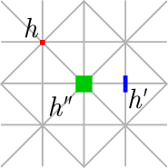
(b) In $\mathbb{K}^{2}$.

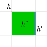
(c) In $\mathcal{P}(\mathbb{R}^{2})$.

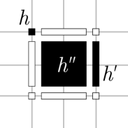
(d) In $\mathbb{H}^{2}$.

Figure 2: Three faces, $h,h^{\prime}$ and $h^{\prime\prime}$, depicted as subsets of $\mathbb{Z}^{2}$ (a), as vertices of the Khalimsky grid (b), as geometrical objects, parts of the plane (c), and as elements of the cellular complex $\mathbb{H}^{2}$ (d).

The set of faces of $\mathbb{H}^{n}$ is arranged onto a grid, the so-called Khalimsky’s grid, depicted in gray in Figure 2(b). The set of $n$-faces is denoted by $\mathbb{H}^{n}_{n}$; it is the $n$-Cartesian product of $\mathbb{H}^{1}_{1}$.

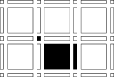
(a) $E\subset\mathbb{H}^{2}$

(b) $\mathit{st}(E)$

(c) $\mathit{cl}(E)$

(d) $\mathit{int}(E)$

(e) $\partial E$

(f) $\mathit{ext}(E)$

Figure 3: Some topological operators on subsets of $\mathbb{H}^{n}$.

II-C Set-Valued Maps

Now let us recall the mathematical background relative to set-valued maps [aubin.2008.book]. A set-valued map $~{}\textsc{u}\,:\,X\,\leadsto\,Y\;$ is characterized by its graph, $\,\mathrm{Gra}(\textsc{u})\,=\,\{\,(x,y)\in X\times Y\,|\,y\in\textsc{u}(x)\,\}.$ There are two different ways to define the “inverse” of a subset by a set-valued map: $\,\textsc{u}^{\oplus}(M)\;=\;\{\,x\in X\,|\,\textsc{u}(x)\cap M\neq\emptyset\,\}\,$ is the inverse image of $M$ by u, whereas $\,\textsc{u}^{\ominus}(M)\;=\;\{\,x\in X\,|\,\textsc{u}(x)\subset M\,\}\,$ is the core of $M$ by u. Two distinct continuities are defined on set-valued maps. The one we are interested in is the “natural” extension of the continuity of a single-valued function. When $X$ and $Y$ are metric spaces and when $\,\textsc{u}(x)\,$ is compact,  u  is said to be upper semi-continuous (USC) at $\,x\,$ if $\,\forall\varepsilon>0,\;\exists\,\eta>0\,$ such that $\,\forall\,x^{\prime}\in B_{X}(x,\eta),\;\textsc{u}(x^{\prime})\subset B_{Y}(\textsc{u}(x),\varepsilon),\,$ where $B_{X}(x,\eta)$ denotes the ball of $X$ of radius $\eta$ centered at $x$. One characterization of USC maps is the following:  u  is USC if and only if the core of any open subset is open.

(a) Image $u:\mathbb{Z}^{2}\rightarrow\mathbb{Z}$

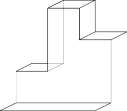
(b) Surface of $u$

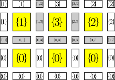
(c) Image $U:\mathbb{H}^{2}\rightarrow\mathbb{I}_{\mathbb{Z}}$

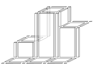
(d) $U$ seen in 3D

Figure 4: From the classical view to the topographical view: In (a), a 2D image $u$ made of six pixels. In (b), it topographical view (where discontinuities can be observed). In (c), the USC span-based immersion $U$ of $u$ where the 2-faces (elements of $\mathbb{H}^{2}_{2}$) are depicted in yellow; they correspond to the pixels of $u$. In (d), the topographical view of the USC map $U$ without discontinuities (in the sense of an USC map).

A topographical view of a 2D image can be observed in Figure 4 and shows that, using span-based immersion maps, we obtain “continuous” maps (in the sense of set-valued maps).

II-D Interpolation

We are going to immerse a discrete $n$-D function defined on a cubical grid $\,u:\mathbb{Z}^{n}\rightarrow\mathbb{Z}\,$ into some larger spaces in order to get some continuity properties. For the domain space, we use the subdivision $X=\frac{1}{2}\mathbb{H}^{n}$ of $\mathbb{H}^{n}$. Every element $z\in\mathbb{Z}^{n}$ is mapped to an element $\,m(z)\in\frac{1}{2}\mathbb{H}^{n}_{n}\,$ of dimension $n$ with $z=(z_{1},\ldots,z_{n})~{}\longmapsto~{}m(z)\,=\,\{z_{1},z_{1}+\frac{1}{2}\}\times\ldots\times\{z_{n},z_{n}+\frac{1}{2}\}$. The definition domain of $u$, $\mathcal{D}\subseteq\mathbb{Z}^{n}$, has thus a counterpart in $X$, that will also be denoted $\mathcal{D}$, and that is depicted in bold in Figure 6.

For the value space, we immerse $\mathbb{Z}$ (the set of pixel values) into the larger space $Y=\frac{1}{2}\mathbb{H}^{1}$, where every integer becomes a closed singleton, that is, an element of $\mathbb{H}^{1}_{0}$. Thanks to an “interpolation” function, we can now define from $u$ a set-valued map $\textsc{u}=\mathfrak{I}(u)$. We have $~{}\textsc{u}\,:\,X\,\leadsto\,Y\,$ and we set $\forall\,h\in X,\;\;\textsc{u}(h)\,:=\,$

$$\left\{\begin{array}[]{ll}\{\,u(m^{-1}(h))\,\}&\mbox{~{}~{}if ~{}}h\in\mathcal{D}\\ {}\max(\,\textsc{u}(h^{\prime}):\,h^{\prime}\in\mathit{st}(\mathit{cl}(h))\cap\mathcal{D}\,)&\mbox{~{}~{}if ~{}}h\in\frac{1}{2}\mathbb{H}^{n}_{1}\backslash\mathcal{D}\\ {}\mathrm{span}(\,\textsc{u}(h^{\prime}):\,h^{\prime}\in\mathit{st}(h)\cap\mathcal{D}\,)&\mbox{~{}~{}if ~{}}h\in X\backslash\frac{1}{2}\mathbb{H}^{n}_{1}.\end{array}\right.$$

(a) Primary image $u$.

(b) Subdivided image $u_{s}$.

(c) Immersed image u.

Figure 5: A grayscale 2D image $u$ which is not well-composed since any value in $[0,1]$ is lower than any value in $[3,4]$, a representation $u_{s}$ of $u$ which is well-composed thanks to the max-interpolation, and the corresponding well-composed immersion $U$ of $u_{s}$ into $\mathbb{H}^{2}$.

$[\,\textsc{u}\,\lhd\,4\!-\!\epsilon\,]$	$[\,\textsc{u}\,\lhd\,2\!-\!\epsilon\,]$	$[\,\textsc{u}\,\rhd\,1\!-\!\epsilon\,]$	$[\,\textsc{u}\,\rhd\,3\!-\!\epsilon\,]$
$[u_{s}<4]$	$[u_{s}<2]$	$[u_{s}\geq 1]$	$[u_{s}\geq 3]$
$[u<4]$	$[u<2]$	$[u\geq 1]$	$[u\geq 3]$

Figure 6: Since we have used the max-interpolation to make $u$ well-composed, the lower threshold sets of the immersion $U$ are connected, or equivalently the lower threshold sets of $u_{s}$ are connected, iff the lower threshold sets of $u$ are $2n$-connected. Conversely, the upper threshold sets of $U$ are connected, or equivalently the upper threshold sets of $u_{s}$ are connected, iff the threshold sets of $u$ are $(3^{n}-1)$-connected. We have chosen here $\epsilon=\frac{1}{2}$ because we work with integral values. Recall that in well-composed images, $2n$- and $(3^{n}-1)$-connectivities are equivalent [boutry.15.ismm].

An example of interpolation is given in Figure 5. Actually, whatever $u$, such a discrete interpolation $\mathfrak{I}(u)$ can also be interpreted as a non-discrete set-valued map $\mathfrak{I}_{\mathbb{R}}(u):\mathbb{R}^{n}\leadsto\mathbb{R}$ (schematically $\mathfrak{I}_{\mathbb{R}}(u)(x)=\mathfrak{I}(u)(h)$ with $h$ such as $x\in\mathbb{R}^{n}$ falls in $h\in\frac{1}{2}\mathbb{H}^{n}$), and we can show that $\mathfrak{I}_{\mathbb{R}}(u)$ is an upper semi-continuous [aubin.2008.book] (shortly USC) map.

Such span-based immersions will be called $\mathcal{SI}$-maps in the sequel.

II-E Discrete surfaces and well-composedness

Let us recall the definition of discrete surfaces [najman2013discrete]. Let $Y$ be some partially ordered set (shortly poset) of rank $n\geq 0$. Let $X$ be some subset of $Y$. We say that $X$ is a discrete $(-1)$-surface when $X=\emptyset$. We say $X$ is a $0$-surface if it can be written $\{h,h^{\prime}\}$ with $h\not\in st_{Y}(h^{\prime})\cup cl_{Y}(h^{\prime})$. We call $X$ a $k$-surface with $k\geq 1$ when it is connected and when for any $h\in X$, the poset $st_{Y}(h)\cup cl_{Y}(h)\setminus\{h\}$ is a discrete $(k-1)$-surface.

Furthermore, we call (combinatorial) boundary of a subset $Z$ of $Y$ the set:

$$\partial Z:=cl_{Y}(Z)\cap cl_{Y}(Y\setminus Z).$$

We say that $Z$ is (Alexandrov) well-composed (shortly WC) when its boundary is a (possibly empty) separated union of discrete $(n-1)$-surfaces.

Remark 1.

We recall that the shapes of a WC $\mathcal{SI}$-map are WC too.

II-F The tree of shapes in $\mathbb{H}^{n}$

Assuming that the domain $X$ of the interpolation $\mathfrak{I}(u)$ is unicoherent), like $\mathbb{H}^{n}/2$ or any hyper-rectangle in $\mathbb{H}^{n}/2$, and that it set $Y$ of values is $\mathbb{H}^{1}/2$. Then, threshold sets are defined for any $\lambda\in Y$ in this way [boutry2019make, boutry.15.ismm]:

$$\,[\,\textsc{u}\,\lhd\,\lambda\,]\,=\,\{\,x\in X\,\,|\,\,\forall\,\mu\in\textsc{u}(x),\;\mu<\lambda\,\}\,$$

$$\,[\,\textsc{u}\,\rhd\,\lambda\,]\,=\,\{\,x\in X\,\,|\,\,\forall\,\mu\in\textsc{u}(x),\;\mu>\lambda\,\}.$$

We can show (see [najman.2013.ismm]) that, for any $\lambda\in Y$, the threshold sets $[\,\mathfrak{I}(u)\,\lhd\,\lambda\,]$ and $[\,\mathfrak{I}(u)\,\rhd\,\lambda\,]$ are well-composed [latecki1995well] when we use a well-composed interpolation $\mathfrak{I}(u)$ (see [boutry.15.ismm, najman.2013.ismm] for examples of $n$-D well-composed interpolations). Then the combinatorial boundaries of the threshold sets are discrete surfaces. By defining respectively the upper and the lower shapes:

$$\mathcal{S}_{\triangleright}=\left\{\,\mathrm{Sat}(\Gamma);\;\Gamma\in\{\mathcal{CC}([\,\mathfrak{I}(u)\,\rhd\,\lambda\,])\}_{\lambda}\,\right\},$$

$$\mathcal{S}_{\triangleleft}=\left\{\,\mathrm{Sat}(\Gamma);\;\Gamma\in\{\mathcal{CC}([\,\mathfrak{I}(u)\,\lhd\,\lambda\,])\}_{\lambda}\,\right\},$$

we obtain then that together these shapes form a set of shapes $\mathfrak{S}_{\mathfrak{I}(u)}$ which is a tree, the tree of shapes.

II-G Some elementary properties about shapes

The following properties of shapes will be useful in the sequel.

Proposition 1 (Lemma 2.5 in [caselles2009geometric]).

Let $\mathcal{D}$ be a topological space. Then, the $\mathrm{Sat}$ operator is monotonic, that is, for any subset $A,B$ of $\mathcal{D}$:

$$A\subseteq B\Rightarrow\mathrm{Sat}(A)\subseteq\mathrm{Sat}(B).$$

Proposition 2 (Lemma 2.4 [caselles2009geometric]).

Let $\mathcal{D}$ be a topological space. Then, when $A\subseteq\mathcal{D}$ is an open set, then $\mathrm{Sat}(A)$ is open too.

Proposition 3 (Lemma 2.7 [caselles2009geometric]).

Let $\mathcal{D}$ be a topological space. Then, when $A\subseteq\mathcal{D}$ is connected, then $\mathrm{Sat}(A)$ is connected too.

Proposition 4 (Lemma 2.10 [caselles2009geometric]).

Let $\mathcal{D}$ be a compact, locally connected, and unicoherent topological space. Let $A$ be a subset of $\mathcal{D}$ such that $\mathrm{Sat}(A)\neq\mathcal{D}$. Then $\mathrm{Sat}(A)\subseteq\mathrm{Sat}(\partial A)$. Furthermore, if $A$ is closed, $\mathrm{Sat}(A)=\mathrm{Sat}(\partial A)$.

Figure 7: The closure and saturation operators do not always commute when the used image is not well-composed (see the pinch encircled in red on the left side which causes this topological issue).

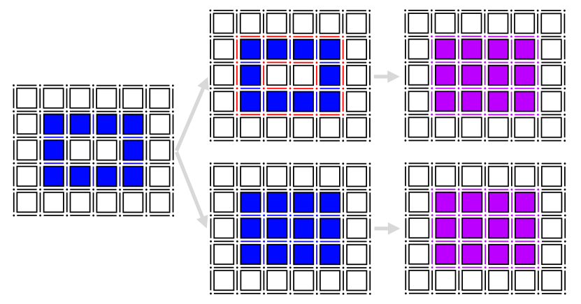
Figure 8: The closure and saturation operators commute when the used image is well-composed.

Proposition 5 ([najman2013discrete]).

Let $\mathcal{D}$ be a $n$-D finite (unicoherent) hyper-rectangle in the $n$-D Khalimsky grid, and let $p_{\infty}$ be a $n$-face of $\mathcal{D}$ which belongs to $\partial\mathcal{D}$. When a finite set $X$ is an open regular WC set, then we have the following property for any $x\in\mathcal{D}$:

$$\mathrm{Sat}(cl_{\mathcal{D}}(X),x)=cl_{\mathcal{D}}(\mathrm{Sat}(X,x)).$$

Figures 7 and 8 depict the possible topological issue which arises when we do not work with well-composed images.

III Algorithm Description

III-A The main algorithm

$$\begin{array}[]{rcccl}&u&\xrightarrow{~{}~{}\mbox{\scriptsize immersion}~{}~{}}&\textsc{u}&\vskip 6.0pt plus 2.0pt minus 2.0pt\\ \mbox{\scriptsize tree of shapes}&\Big{\downarrow}&&\Big{\downarrow}&\mbox{\scriptsize tree computation}\vskip 6.0pt plus 2.0pt minus 2.0pt\\ &\mathfrak{S}(u)&\xleftarrow{~{}~{}\mbox{\scriptsize emersion}~{}~{}}&\mathfrak{S}(\textsc{u})&\end{array}$$

Figure 9: Global scheme to compute the tree of shapes. The “tree computation” on the right side is composed of the two steps: sort (propagation) and union-find (effective tree computation thanks to the $\mathit{parent}$ relationship).

Let us begin with an intuitive explanation of the computation of the tree of shapes (see Figure 9). We start from an image $u$ whose domain is a subset of $\mathbb{Z}^{n}$. Then, we compute in $\mathbb{Z}^{n}/2$ its well-composed max-interpolation. Then, we immerse the interpolation into the $n$-D Khalimsky grid, so we provide some continuity to the new image u representing $u$. We call abusively this procedure the immersion step. Then, based on u, we add a border, from which we start the propagation, and we go deeper and deeper in the image, until we have covered the whole domain of the image. This step is called the tree computation because while we cover the domain of the image, we can deduce the parenthood relationship between the components in the image (we prove it in the next section). Since the propagation has been done over a domain which has been subdivided twice (once with the max interpolation and once to immerse $\mathbb{Z}^{n}/2$ into $\mathbb{H}^{n}/2$), we have to go back to the initial domain. This last step is called the emersion and removes the secondary pixels to keep only the primary pixels.

III-B The main procedure of the algorithm more in details

1  compute_ql_tree ($u$) : Pair(T, Array[P])

2 begin

3       u $\leftarrow$ immersion(u)

4       ($\mathcal{R}$, $u^{\flat}$) $\leftarrow$ sort(u)

5       $\mathit{parent}$ $\leftarrow$ union_find($\mathcal{R}$)

6       canonicalize_tree($\mathit{parent}$, $\mathcal{R}$, $u^{\flat}$)

7       ($\mathit{parent}$’, $\mathcal{R}$’) $\leftarrow$ emerge($\mathit{parent}$, $\mathcal{R}$, $u^{\flat}$)

8       return ($\mathit{parent}$’, $\mathcal{R}$’)

9      

10

 

Algorithm 1 The quasi-linear computation of the tree of shapes (main procedure).

The algorithmic description of the procedure presented in the previous subsection is as described in Alg. 1. We start with the procedure called immersion, and we follow with the computation of the tree of shapes in three steps: $(1)$ We use a front propagation algorithm sort which handles a hierarchical queue and starts from the border of the image and covers progressively the whole domain, it outputs then an array $\mathcal{R}$ of the ordered pixels of the domain of the image, $(2)$ Now that we have $\mathcal{R}$, we use union_find to deduce the parenthood relationship $\mathit{parent}$ between the pixels of the image, that is, it builds the tree of shapes (but without optimization) of u; $(3)$Then the procedure canonicalize_tree is utilized to optimize the tree so that each pixel has a parent which is the representative of the component it belongs to. This way, we obtain $\mathit{parent}$ which is in fact $\mathfrak{S}(U)$. From it, we can easily deduce $\mathfrak{S}(u)$ by removing the secondary pixels (see the emerge prodecure).

III-C The sorting step

11  

12priority_push($q,\,n,\,U,\,\mathscr{L}$)

13 /* modify $q$ */

14 begin

15       $[\mathit{lower},\,\mathit{upper}]\leftarrow U(n)$

16       if $\mathscr{L}<\mathit{lower}$ then

17             $\mathscr{L}^{\prime}\leftarrow\mathit{lower}$

18            

19      else if $\mathscr{L}>\mathit{upper}$ then

20             $\mathscr{L}^{\prime}\leftarrow\mathit{upper}$

21            

22      else

23             $\mathscr{L}^{\prime}\leftarrow\mathscr{L}$   /* we have $\mathscr{L}\in U(n)$ */

24            

25      $\textsc{push}(q[\mathscr{L}^{\prime}],n)$

26      

27

28

29priority_pop(q,   $\mathscr{L}$) : H

30 /* modify $q$, and sometimes $\ell$ */

31 begin

32       if $q[\mathscr{L}]$ is empty then

33             $\mathscr{L}^{\prime}\leftarrow$ level next to $\mathscr{L}$ such as $q[\mathscr{L}^{\prime}]$ is not empty

34             $\mathscr{L}\leftarrow\mathscr{L}^{\prime}$

35            

36      return $\textsc{pop}(q[\mathscr{L}])$

37      

38

39

40sort($U$) : Pair(Array[H], Image)

41 begin

42       for all h do

43             $\mathit{deja\_vu}(h)\leftarrow\mathrm{false}$

44            

45      $\mathit{idx}\leftarrow 0$   /* index in $\mathcal{R}$ */

46       $\mathscr{L}_{\infty}\leftarrow U(p_{\infty})$

47       $\textsc{push}(q[\mathscr{L}_{\infty}],\,p_{\infty})$

48       $\mathit{deja\_vu}(p_{\infty})\leftarrow\mathrm{true}$

49       $\mathscr{L}\leftarrow\mathscr{L}_{\infty}$   /* start from root level */

50       while $q$ is not empty do

51             $h\leftarrow\textsc{priority\_pop}(q,\,\mathscr{L})$

52             $u^{\flat}(h)\leftarrow\mathscr{L}$

53             $\mathcal{R}[\mathit{idx}]\leftarrow h$

54             $\mathit{idx}\leftarrow\mathit{idx}+1$

55             for all $n\in\mathcal{N}(h)\textup{{ such as}}\ \mathit{deja\_vu}(n)=\mathrm{false}$ do

56                   $\textsc{priority\_push}(q,\,n,\,U,\,\mathscr{L})$

57                   $\mathit{deja\_vu}(n)\leftarrow\mathrm{true}$

58                  

59            

60      return ($\mathcal{R}$, $u^{\flat}$)

61

62

 

Algorithm 2 The front propagation algorithm sorting the pixels.

The details of the sorting step can be found in Alg 2. To sort the faces of the domain $X$ of $U$, we use a classical front propagation based on a hierarchical queue [meyer.1991.afcet], denoted by $q$, the current level being denoted by $\mathscr{L}$. There are two notable differences with the well-known hierarchical-queue-based propagation. First the $d$-faces, with $d<n$, are interval-valued so we have to decide at which (single-valued) level to enqueue those elements. The solution is straightforward: a face $h$ is enqueued at the value of the interval $U(h)$ that is the closest to $\mathscr{L}$ (see the procedure priority_push). Just also note that we memorize the enqueuing level of faces thanks to the image $u^{\flat}$ (see the procedure sort). Second, when the queue at current level, $q[\mathscr{L}]$, is empty (and when the hierarchical queue $q$ is not yet empty), we shall decide what the next level to be processed is. We have the choice of taking the next level, either less or greater than $\mathscr{L}$, such that the queue at that level is not empty (see the procedure priority_pop), even if this choice has no influence on the result $\mathcal{R}$ of the algorithm. The image $U$, in addition with the browsing of level in the hierarchical queue, allows for a propagation that is “continuous” both in domain space and in level space.

III-D Tree Representation

63  

64find_root($\mathit{zpar},x$) : P /* modify $\mathit{zpar}$ */

65 begin

66       if $\mathit{zpar}$ (x) = x then

67             return $x$

68      else

69             $\mathit{zpar}(x)\leftarrow\textsc{find\_root}(\mathit{zpar},\mathit{zpar}(x))$

70             return $\mathit{zpar}(x)$

71      

72

73

74do_union($p^{\prime},\,r^{\prime}$)

75 /* modify $\mathit{zpar}$, $\mathit{rank}$, and $\mathit{last}$ */

76 begin

77       if $\mathit{rank}(p^{\prime})>\mathit{rank}(r^{\prime})$ then

78             /* new root is $p^{\prime}$ */

79             $\mathit{zpar}(r^{\prime})\leftarrow p^{\prime}$

80             if $\mathit{last}(r^{\prime})<\mathit{last}(p^{\prime})$ then

81                   $\mathit{last}(p^{\prime})\leftarrow\mathit{last}(r^{\prime})$

82            

83      else

84             /* new root is $r^{\prime}$ */

85             $\mathit{zpar}(p^{\prime})\leftarrow r^{\prime}$

86             if $\mathit{last}(p^{\prime})<\mathit{last}(r^{\prime})$ then

87                   $\mathit{last}(r^{\prime})\leftarrow\mathit{last}(p^{\prime})$

88            if $\mathit{rank}(p^{\prime})=\mathit{rank}(r^{\prime})$ then

89                   $\mathit{rank}(r^{\prime})\leftarrow\mathit{rank}(r^{\prime})+1$

90            

91      

92

93

94union_find($\mathcal{R}$) : T

95 /* with tree balancing and compression */

96 begin

97       for all p do

98             $\mathit{zpar}(p)\leftarrow\mathrm{undef}$

99             $\mathit{rank}(p)\leftarrow 0$

100      for $\mathit{idx}\leftarrow N-1$ to 0 do

101             $p\leftarrow\mathcal{R}[\mathit{idx}]$   /* $p$ goes from leaves to root */

102             $\mathit{parent}(p)\leftarrow p$

103             $\mathit{zpar}(p)\leftarrow p$

104             $\mathit{last}(p)\leftarrow\mathit{idx}$

105             for all $n\in\mathcal{N}(p)\textup{{ such as}}\ \mathit{zpar}(n)\neq\mathrm{undef}$ do

106                   $p^{\prime}\leftarrow\textsc{find\_root}(\mathit{zpar},p)$

107                   $r^{\prime}\leftarrow\textsc{find\_root}(\mathit{zpar},n)$

108                   if $r^{\prime}\neq p^{\prime}$ then

109                         $r\leftarrow\mathcal{R}[\,last(r^{\prime})\,]$

110                         $\mathit{parent}(r)\leftarrow p$

111                         $\textsc{do\_union}(p^{\prime},r^{\prime})$   /* update $\mathit{zpar}$ */

112                        

113                  

114            

115      /* deallocate $\mathit{zpar}$, $\mathit{rank}$, and $\mathit{last}$ */

116       return $\mathit{parent}$

117

118

 

Algorithm 3 Tree construction based on the ancestor relationship $\mathcal{R}$.

The max-tree algorithm presented in [berger.2007.icip] is actually a kind of meta-algorithm that can be “filled in” so that it can serve different aims; in particular, in the present paper, it gives an algorithm to compute the tree of shapes. An extremely simple union-find structure (attributed by Aho to McIlroy and Morris) was shown by Tarjan [tarjan.1975.jacm] to be very efficient. This structure, also called disjoint-set data structure or merge-find set, has many advantages that are detailed in [carlinet.2013.ismm]; amongst them, memory compactedness, simplicity of use, and versatility. This structure and its related algorithms are of prime importance to handle connected operators [meijster.2002.pami, geraud.2005.ismm].

Figure 10: Building the max-tree (left side) and the tree of shapes (right side) from root to leaves using the array $\mathcal{R}$ (figure extracted from [geraud.2013.ismm]).

Let us denote by $\mathcal{R}$ the ancestor relationship in trees: we have $a\,\mathcal{R}\,p$ iff $a$ is an ancestor of $p$. $\mathcal{R}$ can be encoded as an array of elements (nodes) so that $a\,\mathcal{R}\,p\,\Leftrightarrow\,\mathit{index}_{\mathcal{R}}(a)<\mathit{index}_{\mathcal{R}}(p)$; browsing that array thus corresponds to a downwards browsing of the tree, i.e., from root to leaves. To construct the max-tree of a given image, we rely on a rooted tree defined by a parenthood function, named $\mathit{parent}$, and encoded as an $n$-D image (so $\mathit{parent}(p)$ is an $n$-D point). When a node of the max-tree contains several points, we choose its first point (with respect to $\mathcal{R}$) as the representative for this node; that point is called a component “canonical point” or a “level root”. Let $\Gamma$ denote a component corresponding to a node of the max-tree, $p_{\Gamma}$ its canonical element, and $p_{r}$ the root canonical element. The $parent$ function that we want to construct should verify the following four properties:

1. $\,\mathit{parent}(p_{r})=p_{r}\,$;

2. $\,\forall\,p\neq p_{r},\;\mathit{parent}(p)\,\mathcal{R}\,p\,$;

3. $\,p$ is a canonical element iff

   $$\,\{p=p_{r}\}\,\vee\,\{u(\mathit{parent}(p))\neq u(p)\}\,;$$

4. $\,\forall p,p\in\Gamma\Leftrightarrow\{u(p)=u(p_{\Gamma})\}\wedge\{\exists\,i,\mathit{parent}^{i}(p)=p_{\Gamma}\}.$

119  canonicalize($\mathit{parent},\mathcal{R}$, $u^{\flat}$)

120 /* modify $\mathit{parent}$ */

121 begin

122       for $\mathit{idx}\leftarrow 0$ to $N-1$ do

123             $p\leftarrow\mathcal{R}[\mathit{idx}]$   /* $p$ goes from root to leaves */

124             $p^{\prime}\leftarrow\mathit{parent}(p)$

125             if $u^{\flat}(\mathit{parent}(p^{\prime}))=u^{\flat}(p^{\prime})$ then

126                   $\mathit{parent}(p)\leftarrow\mathit{parent}(p^{\prime})$

127                  

128            

129      

130

 

Algorithm 4 Canonicalization.

The routine union_find, given in Algorithm 3, is the classical “union-find” algorithm [tarjan.1975.jacm] but modified so that it computes the expected morphological tree [berger.2007.icip] while browsing pixels following $\mathcal{R}^{-1}$ (see Figure 10), i.e., from leaves to root. Its result is a $\mathit{parent}$ function that fulfills those first four properties. Obtaining the following extra property, “5. $\,\forall p,\;\mathit{parent}(p)\,$ is a canonical element,” is extremely interesting since it ensures that the parent function, when restricted to canonical elements only, gives a “compact” morphological tree. Precisely it allows to browse components while discarding their contents: a traversal is thus limited to one element (one pixel) per component, instead of passing through every image elements (pixels). Transforming the parent function so that property 5 is verified can be performed by a simple post-processing of the union-find computation. The resulting tree has now the simplest form that we can expect (see Alg. 4); furthermore we have an isomorphism between images and their canonical representations.

The algorithm presented in [berger.2007.icip] to compute the max-tree is also able to compute the tree of shapes. The skeleton of this algorithm is the routine compute_tree is composed of the steps presented above. In the case of the max-tree, the sorting step provides $\mathcal{R}$ encoded as an array of points sorted by increasing gray-levels in $u$, i.e., such that the array indices satisfy $~{}\mathit{idx}<\mathit{idx}^{\prime}\;\Rightarrow\;u(\mathcal{R}[\mathit{idx}])\leq u(\mathcal{R}[\mathit{idx}^{\prime}])$. Last, the canonicalization post-processing is trivial [berger.2007.icip]. In the case of the tree of shapes, it is also a tree that represents an inclusion relationship between connected components of the input image. As a consequence an important idea to catch is that the tree of shapes can be computed with the exact same routine, union_find, as the one used by the max-tree. The major and crucial difference between the max-tree and the tree of shapes computations is obviously the sorting step (see Figure 10). For the union_find routine to be able to compute the tree of shapes using $\mathcal{R}^{-1}$, the sort routine has to sort the image elements so that $\mathcal{R}$ corresponds to a downward browsing of the tree of shapes. Schematically, $\mathcal{R}$ contains the image pixels going from the “external” shapes to the “internal” ones (included in the former ones).

III-E The last step: the emersion

131  

132is_representative($x$) : $\mathbb{B}$

133 begin

134       return $\mathit{parent}(x)=x~{}\textbf{or~{}}u^{\flat}(\mathit{parent}(x))\neq u^{\flat}(x)$

135

136

137get_representative($x$) : P

138 begin

139       while $\textbf{not~{}}\textsc{is\_representative}(x)$ do

140             $x\leftarrow\mathit{parent}(x)$

141            

142      return $x$

143

144

145find_primary_ancestor($x$) : P

146 begin

147       repeat

148             $x\leftarrow\mathit{parent}(x)$

149            

150      until $\textbf{not~{}}\textsc{is\_primary}(x)~{}\textbf{and~{}}\mathit{parent}(x)\neq x$

151      return $x$

152

153

154emerge($\mathit{parent}$, $\mathcal{R}$, $u^{\flat}$)

155 begin

156       /* rearrange */

157       for $i\leftarrow 0$ to $N-1$ do

158             $p\leftarrow\mathcal{R}[i]$   /* $p$ goes from root to leaves */

159             if $\textsc{is\_representative}(p)$ then

160                   continue

161                  

162            $p^{\prime}\leftarrow\textsc{get\_representative}(p)$

163             if $\textbf{not~{}}\textsc{is\_primary}(p^{\prime})~{}\textbf{and~{}}\textsc{is\_primary}(p)$ then

164                   if $\mathit{parent}(p^{\prime})=p^{\prime}$ then

165                         $\mathit{parent}(p)\leftarrow p$

166                        

167                  else

168                         $\mathit{parent}(p)\leftarrow\mathit{parent}(p^{\prime})$

169                        

170                  $\mathit{parent}(p^{\prime})\leftarrow p$

171                  

172            

173      

174      /* keep only primary points */

175       $j\leftarrow 0$

176       for $i\leftarrow 0$ to $N-1$ do

177             $p\leftarrow\mathcal{R}[i]$   /* $p$ goes from root to leaves */

178             if $\textsc{is\_primary}(p)$ then

179                   $\mathcal{R}[j]\leftarrow p$

180                   $j\leftarrow j+1$

181                   $\mathit{parent}(p)\leftarrow\textsc{find\_primary\_ancestor}(p)$

182                  

183            

184      $N\leftarrow j$

185      

186      /* canonicalization */

187       canonicalize($\mathit{parent},\mathcal{R}$, $u^{\flat}$)

188      

189      return ($\mathit{parent}$, $\mathcal{R}$)

190

191

 

Algorithm 5 Emersion procedure used to obtain the final tree (in the domain of the initial image).

Using the canonicalized tree, we can finalize the procedure and emerge the connected components of the tree simply by removing the secondary pixels of the components (see Algo 5).

IV The $n$-D proof

IV-A New mathematical properties

Let us recall that the strict threshold sets of a plain map are open sets.

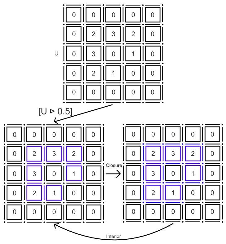
Figure 11: Any strict threshold set of a $\mathcal{SI}$-map is regular

Proposition 6.

Let $U$ be some $\mathcal{SI}$-map on a $n$-D Khalimsky grid, then any of its strict threshold sets $T$ is regular, that is, it satisfies:

$$\mathrm{Int}(\mathit{cl}_{\bar{\mathcal{D}}}({T}))=T.$$

The direct consequence is that its strict shapes are regular sets too.

Proof:

Let us treat the upper case (see Figure 11) for some value $\lambda\in\mathbb{R}$ (the lower case follows the same reasoning). Let $\lambda$ be some real value, and $[U\rhd\lambda]$ the corresponding lower set. Now, let us prove its regularity using a double inclusion. First, for any $\lambda\in\mathbb{R}$, $[U\rhd\lambda]$ is contained in $\mathit{cl}_{\bar{\mathcal{D}}}({[U\rhd\lambda]})$, thus $[U\rhd\lambda]=\mathrm{Int}([U\rhd\lambda])\subseteq\mathrm{Int}(\mathit{cl}_{\bar{\mathcal{D}}}({[U\rhd\lambda]}))$, which proves the first inclusion. Second, let us define some $z\in\mathrm{Int}(\mathit{cl}_{\bar{\mathcal{D}}}({[u\rhd\lambda}))$, then $\mathit{st}_{\bar{\mathcal{D}}}({z})\subseteq\mathit{cl}_{\bar{\mathcal{D}}}({[U\rhd\lambda]})$. The subset $(\mathit{st}_{\bar{\mathcal{D}}}({z}))_{n}$ made of the $n$-faces of $\mathit{st}_{\bar{\mathcal{D}}}({z})$ is contained in $\mathit{cl}_{\bar{\mathcal{D}}}({[U\rhd\lambda]})=\partial[U\rhd\lambda]\sqcup[U\rhd\lambda]$ (disjoint union). Since $\partial[U\rhd\lambda]$ does not contain any $n$-face (as every combinatorial boundary), then:

$$(\mathit{st}_{\bar{\mathcal{D}}}({z}))_{n}\subseteq[U\rhd\lambda].$$

Consequently, for any $p\in(\mathit{st}_{\bar{\mathcal{D}}}({z}))_{n}$, $U(p)\rhd\lambda$, which leads by using the formula of the span-based immersion to:

$$U(z):=\mathrm{span}\{U(p)\;;\;p\in(\mathit{st}_{\bar{\mathcal{D}}}({z}))_{n}\}\rhd\lambda,$$

then $U(z)\rhd\lambda$, that is, $z\in[U\rhd\lambda]$. The proof is done.

Figure 12: Boundaries in red of some subsets of $\mathbb{H}^{2}$.

Figure 13: Internal boundaries (in black square encircled in red) of some subsets of $\mathbb{H}^{2}$; the $n$-faces remaining after having removed the internal boundaries to their respective sets are encircled in yellow to show the thickness of the internal boundaries.

Definition 1 (Interior boundaries).

Let $\mathbb{H}^{n}$ be the $n$-D Khalimsky grid, and let $F$ be an open subset of $\mathbb{H}^{n}$. We call interior boundary of $F$ the set $\partial_{\mathrm{int}}F=st_{\mathbb{H}^{n}}(\partial F)\cap F$.

We recall that a family $\bigcup_{i\in I}X_{i}$ of subsets of a poset $X$ is said to be a separated union when for any $i,j$ in $I$ with $i\neq j$, $(st_{X}(X_{i})\cup cl_{X}(X_{i}))\cap X_{j}=\emptyset$.

IV-B Property of the internal boundaries

Proposition 7.

Let $\mathcal{T}$ be an open subset of $\mathbb{H}^{n}$. The set $\partial_{\mathrm{int}}(\mathcal{T})$ can be reformulated this way:

$$\partial_{\mathrm{int}}(\mathcal{T})=st_{\mathbb{H}^{n}}(\mathcal{T})\cap st_{\mathbb{H}^{n}}(\mathbb{H}^{n}\setminus\mathcal{T}).$$