LTL-Transfer: Skill Transfer for Temporally-Extended Task Specifications

Abstract

Deploying robots in real-world domains, such as households and flexible manufacturing lines, requires the robots to be taskable on demand. Linear temporal logic (LTL) is a widely-used specification language with a compositional grammar that naturally induces commonalities across tasks. However, the majority of prior research on reinforcement learning with LTL specifications treats every new formula independently. We propose LTL-Transfer, a novel algorithm that enables subpolicy reuse across tasks by segmenting policies for training tasks into portable transition-centric skills capable of satisfying a wide array of unseen LTL specifications while respecting safety-critical constraints. Experiments in a Minecraft-inspired domain show that LTL-Transfer can satisfy over 90% of 500 unseen tasks after training on only 50 task specifications and never violating a safety constraint. We also deployed LTL-Transfer on a quadruped mobile manipulator in an analog household environment to demonstrate its ability to transfer to many fetch and delivery tasks in a zero-shot fashion.

I Introduction

A key requirement for deploying autonomous agents in many real-world domains is the ability to perform multiple novel potential tasks on demand. These tasks typically share components like the objects and the trajectory segments involved, which creates an opportunity to reuse knowledge across tasks [23]. For example, a service robot on the factory floor might have to fetch the same set of components but in different orders depending on the product being assembled, in which case it should only need to learn to fetch a component once.

Linear temporal logic (LTL) [20] is becoming a popular means of specifying an objective for a reinforcement learning agent [17, 24, 6]. Its compositional grammar reflects the compositional nature of most tasks. However, most prior approaches to reinforcement learning for LTL specifications restart learning from scratch for each LTL formula. We propose LTL-Transfer, a novel algorithm that exploits the compositionality inherent to LTL task specifications to enable an agent to maximally reuse policies learned in prior LTL formulas to satisfy new, unseen specifications without additional training. For example, a robot that has learned to fetch a set of components on the factory floor should be able to fetch it in any order. LTL-Transfer also ensures that transferred subpolicies do not violate any safety constraints.

(a) fetch book

(b) deliver juice

Figure 1: The robot is executing four transition-centric skills sequentially to solve a novel task $\mathbf{F}(book\wedge\mathbf{F}(desk_{a}\wedge\mathbf{F}(juice\wedge\mathbf{F}desk_{a})))$, i.e., fetch and deliver a book then a bottle of juice to the user. Two of four skills are shown.

We demonstrated the efficacy of LTL-Transfer in a Minecraft-inspired domain, where the agent can complete over 90% of 500 new task specifications by training on only 50. We then deployed LTL-Transfer on a quadruped mobile manipulator to show its zero-shot transfer ability in an analog household environment when performing fetch and delivery tasks .

II Preliminaries

Linear temporal logic (LTL) for task specification: LTL is a widely used alternative to a numerical reward function for expressing task specifications. An LTL formula $\varphi$ is a Boolean function that determines whether a given trajectory has satisfied the objective expressed by the formula. Littman et al. [17] argue that such task specifications are more natural than numerical reward functions, and they have subsequently been used as a target language for acquiring task specifications in several settings, including from natural language [19] and learning from demonstration [21]. Formally, an LTL formula is interpreted over traces of Boolean propositions over discrete time, and is defined through the following recursive syntax:

$$\varphi:=\alpha\mid\neg\varphi\mid\varphi_{1}\vee\varphi_{2}\mid\mathbf{X}\varphi\mid\varphi_{1}~{}\mathbf{U}~{}\varphi_{2}$$ (1)

Here $\alpha\in AP$ represents a Boolean proposition, mapping a state to a Boolean value; $\varphi,~{}\varphi_{1},~{}\varphi_{2}$ are any valid LTL formulas. The operator $\mathbf{X}$ (next) is used to define a property $\mathbf{X}\varphi$ that holds if $\varphi$ holds at the next time step. The binary operator $\mathbf{U}$ (until) is used to specify ordering constraints. The formula $\varphi_{1}~{}\mathbf{U}~{}\varphi_{2}$ holds if $\varphi_{1}$ holds until $\varphi_{2}$ first holds at a future time instant. The operators $\neg$ (not), and $\vee$ (or) are identical to propositional logic operators. We also utilize the following abbreviated operators: $\wedge$ (and), $\mathbf{F}$ (finally or eventually), and $\mathbf{G}$ (globally or always). $\mathbf{F}\varphi$ specifies that the formula $\varphi$ must hold at least once in the future, while $\mathbf{G}\varphi$ specifies that $\varphi$ must always hold in the future. Consider the Minecraft map depicted in Figure 2. The task of collecting both $wood$ and $axe$ is represented by the LTL formula $\mathbf{F}axe~{}\wedge~{}\mathbf{F}wood$. The task of collecting $wood$ after collecting $axe$ is represented by the formula $\mathbf{F}(axe~{}\wedge~{}\mathbf{F}wood)$. Similarly, the task of collecting $wood$ only once $axe$ has been collected is represented by the formula $\mathbf{F}wood~{}\wedge~{}\neg wood~{}\mathbf{U}~{}axe$.

Every LTL formula can be represented as a Büchi automaton [27, 7] interpreted over an infinite trace of truth values of the propositions used to construct the formula, thus providing an automated translation of a specification into a transition-based representation. We restrict ourselves to the co-safe fragment [14, 18] of LTL that consists of formulas that can be verified by a finite-length trace, thus making it ideal for episodic tasks. Camacho et al. [6] showed that every co-safe LTL formula can be translated into an equivalent reward machine [9, 8] $\mathcal{M}_{\varphi}=\langle\mathcal{Q}_{\varphi},q_{0,\varphi},\mathcal{Q}_{term,\varphi},\varphi,T_{\varphi},R_{\varphi}\rangle$; where $\mathcal{Q}_{\varphi}$ is the finite set of states, $q_{0,\varphi}$ is the initial state, $\mathcal{Q}_{term,\varphi}$ is the set of terminal states; $T_{\varphi}:\mathcal{Q}_{\varphi}\times 2^{AP}\rightarrow\mathcal{Q}_{\varphi}$ is the deterministic transition function; and $R_{\varphi}:\mathcal{Q_{\varphi}}\rightarrow\mathbb{R}$ represents the reward accumulated by entering a given state. LTL-Transfer, our proposed algorithm for transferring learned policies to novel LTL specifications, is compatible with all algorithms that generate policies by solving a product MDP of the reward machine $\mathcal{M}_{\varphi}$ and the task environment.

Options framework: Sutton and Barto [22] introduced a framework for incorporating actions over multiple time steps, called options, into reinforcement learning. An option $o=\langle\mathcal{I},\beta,\pi\rangle$ is defined using the initiation set $\mathcal{I}$, which determines the states where the option can be executed; the termination condition $\beta$, which determines when option execution ends; and the option policy $\pi$. We utilize the options framework to define the task-agnostic skills learned by LTL-Transfer.

III Related work

Most approaches aimed at extending the reinforcement learning paradigm to temporal tasks rely on the automaton equivalent of the LTL formula to augment the state space and generate an equivalent product MDP. Q-learning for reward machines (Q-RM) [6, 9, 8], geometric-LTL (G-LTL) [17], LPOPL [24] are examples of approaches that extend the environment state space with the automaton equivalent to the LTL specification. Notably, Jothimurugan et al. [11] proposed DiRL, an algorithm that interleaves graph-based planning on the automaton with hierarchical reinforcement learning to bias exploration towards trajectories that lead to the successful completion of the LTL specification. However, while these approaches exploit the compositional structure of LTL to speed up learning, they do not exploit the compositionality to transfer to novel task specifications. The policy to satisfy a novel LTL formula must be learned from scratch.

A common approach towards generalization in a temporal task setting has been to learn independent policies for each subtask an agent might perform in the environment [15, 16, 2, 1]. When given a new specification, the agent sequentially composes these policies in an admissible order. Consider the Minecraft-inspired grid world depicted in Figure 2 containing $wood$ and $axe$ objects. The subtask-based approaches would train policies to complete subtasks involving reaching each of these objects. In the case of being tasked with the specification $\varphi_{test}=\mathbf{F}wood~{}\wedge~{}(\neg wood~{}\mathbf{U}~{}axe)$ (i.e., collect $wood$, but do not collect $wood$ until $axe$ is collected), agents trained with the subtask-based approaches would violate the ordering constraint by reaching $axe$ through the grid cells containing $wood$. These approaches rely on additional fine-tuning to correctly satisfy the target task. We propose a general framework for transferring learned policies to novel specifications in a zero-shot setting while preserving the ability to not violate safety constraints.

Our approach draws inspiration from prior works on learning portable skills in Markov domains [12, 10, 3, 4]. These approaches rely on learning a task-agnostic representation of preconditions, constraints, and effects of a skill based on the options framework [22]. We apply this paradigm towards learning portable skills requisite for satisfying temporal specifications.

Kuo et al. [13] proposed learning a modular policy network by composing subnetworks for each proposition and operators. The final policy network is created through the subnetwork modules for a new task specification. Vaeizipoor and Li et al. [25] proposed learning a latent embedding over LTL formulas using a graph neural network to tackle novel LTL formulas. In contrast, our approach utilizes symbolic methods to identify subpolicies best suited for transfer, thus requiring training on orders of magnitude fewer specifications to achieve comparable results. Finally, Xu et al. [28] considered transfer learning between pairs of source and target tasks, while our approach envisions training on a collection of task specifications rather than pairs of source and target tasks.

IV Problem definition

Consider the environment map depicted in Figure 2b. Assume that the agent has trained to complete the specifications to individually collect $axe$ ($\mathbf{F}axe$) and $wood$ ($\mathbf{F}wood$). Now the agent must complete the specification $\varphi_{1}=\mathbf{F}(axe~{}\wedge~{}\mathbf{F}~{}wood)$, i.e., first collect $axe$, then $wood$. The agent should identify that sequentially composing the policies for $\mathbf{F}axe$ and $\mathbf{F}wood$ completes the new task (as depicted in blue). Now consider a different test specification $\varphi_{2}=\mathbf{F}wood~{}\wedge~{}\neg wood~{}\mathbf{U}axe$, i.e., collect $wood$, but avoid visiting $wood$ until $axe$ is collected. Here the agent must realize that policy for $\mathbf{F}axe$ does not guarantee that $wood$ is avoided. Therefore it must not start the task execution using only these two learned skills so as to not accidentally violate the ordering constraint. We develop LTL-Transfer to generate such behavior when transferring learned policies to novel LTL tasks. We begin by formally describing the problem setting.

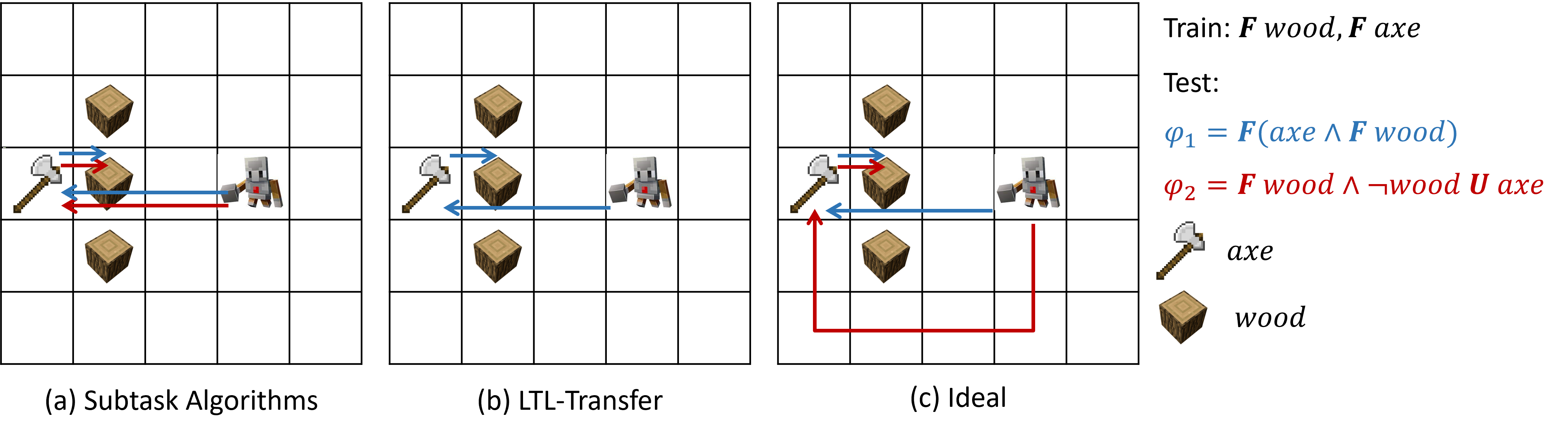
Figure 2: An example 5$\times$5 map in a Minecraft-like grid world. The agent is assumed to have trained on the two training specifications, and is expected to satisfy $\varphi_{1}$ and $\varphi_{2}$. Figure 1a depicts the trajectories adopted by an agent using a subtask-based algorithm (blue for $\varphi_{1}$, red for $\varphi_{2}$). Figure 1b depicts the trajectories followed by LTL-Transfer, our proposed algorithm. Note that LTL-Transfer does not start the task execution for $\varphi_{2}$, as the training task policies do not guarantee the preservation of the ordering constraint. Figure 1c depicts the optimal trajectories for $\varphi_{1}$ and $\varphi_{2}$.

We represent the environment as an MDP without the reward function $\mathcal{M}_{\mathcal{S}}=\langle\mathcal{S},\mathcal{A},T_{\mathcal{S}}\rangle$, where $\mathcal{S}$ is the set of states, $\mathcal{A}$ is the set of actions, and $T_{\mathcal{S}}:\mathcal{S}\times\mathcal{A}\times\mathcal{S}\rightarrow[0,1]$ represents the transition dynamics of the environment. We assume that the learning agent does not have access to the transition dynamics. Further, a set $AP$ of Boolean propositions $\bm{\alpha}$ represents the facts about the environment, and a labeling function $L:\mathcal{S}\rightarrow 2^{AP}$ maps the state to the Boolean propositions. These Boolean propositions are the compositional building blocks for defining the tasks that can be performed within the environment $\mathcal{M}_{\mathcal{S}}$.

We assume that a task within the environment $\mathcal{M}_{\mathcal{S}}$ is defined by a linear temporal logic (LTL) formula $\varphi$, and that the agent is trained on a set of training tasks $\varPhi_{train}=\{\varphi_{1},\varphi_{2},\ldots,\varphi_{n}\}$. We further assume that these policies were learned using a class of reinforcement learning algorithms that operate on a product MDP composed of the environment $\mathcal{M}_{\mathcal{S}}$ and the automaton representing the non-Markov LTL task specification. Q-RM [6, 9, 8], G-LTL [17], LPOPL [24] are examples of such algorithms. LPOPL explicitly allows for sharing policies for specifications that share progression states; therefore, as the baseline best suited for transfer in a zero-shot setting, we choose LPOPL as our learning algorithm of choice.

LTL-Transfer operates in two stages.

1. In the first stage, it accepts the set of training tasks $\varPhi_{train}$ and the learned policies, and outputs a set of task-agnostic, portable options $\mathcal{O}_{e}$.

2. In the second stage, LTL-Transfer identifies and executes a sequence of options to satisfy a novel task specification $\varphi_{test}$ by composing the policies from the set of options $\mathcal{O}_{e}$.

V LTL-Transfer with transition-centric options

An LTL specification $\varphi\in\varPhi_{train}$ to be satisfied is represented as the reward machine $\mathcal{M}_{\varphi}=\langle\mathcal{Q}_{\varphi},q_{0,\varphi},\mathcal{Q}_{term,\varphi},\varphi,T_{\varphi},R_{\varphi}\rangle$. This specification must be satisfied by the agent operating in an environment $\mathcal{M}_{\mathcal{S}}=\langle\mathcal{S},\mathcal{A},T_{\mathcal{S}}\rangle$. The policy learned by LPOPL is Markov with respect to the environment states $\mathcal{S}$ for a given RM state, i.e., the subpolicy to be executed in state $q\in\mathcal{Q}_{\varphi}$, $\pi^{\varphi}_{q}:\mathcal{S}\rightarrow\mathcal{A}$.

An option $o^{\varphi}_{q}$ is executed in the reward machine (RM) state $q$. Our insight is that each of these options triggers a transition in the reward machine on a path that leads towards an acceptance state, and these transitions may occur in multiple tasks. There might be multiple paths through the reward machine to an accepting state; therefore, the target transition of an option $o^{\varphi}_{q}$ is conditioned on the environment state where the option execution was initiated. We propose recompiling each state-centric option, $o^{\varphi}_{q}$, into multiple transition-centric options by partitioning the initiation set of the state-centric option based on the transitions resulting from the execution of the option policy from the starting state. Each resulting transition-centric option will maintain the truth assignments of $AP$ to ensure self-transition until it achieves the truth assignments required to trigger the intended RM transition. These transition-centric options are portable across different formulas. We describe our proposed algorithm in Section V-A.

Given a novel task specification $\varphi_{test}\not\in\varPhi_{train}$, the agent first constructs a reward machine representation of the specification, $\mathcal{M}_{\varphi_{test}}$, then identifies a path through the reward machine that can be traversed by a sequential composition of the options from the set of transition-centric options $\mathcal{O}_{e}$. A key feature of our transfer algorithm is that it is sound and terminating, i.e., if it returns a solution with success, that task execution will satisfy the task specification. Further, it is guaranteed to terminate in finite time if it does not find a sequence of options that can satisfy a given task. We describe the details of this planning algorithm in Section V-B.

The key advantage of this approach is that the compilation of options can be computed offline for any given environment, and the options can then be transferred to novel specifications at execution time. Thus learning to satisfy a limited number of LTL specifications can help satisfy a wide gamut of unseen LTL specifications.

V-A Compilation of transition-centric options

The policy learned by LPOPL to satisfy a specification $\varphi$ identifies the current reward machine state $q\in\mathcal{Q}_{\varphi}$ the task is in and executes a Markov policy $\pi^{\varphi}_{q}$ until the state of the reward machine progresses. This subpolicy can be represented as an option, $o^{\varphi}_{q}=\langle\mathcal{S},\beta_{e^{\varphi}_{q,q}},\pi^{\varphi}_{q}\rangle$; where the initiation set is the entire state space of the task environment; the option terminates when the truth assignments of the propositions $\bm{\alpha}$ do not satisfy the self-transition, represented by the Boolean function $\beta_{e}$ defined as follows,

$$\beta_{e}=\begin{cases}1,&\text{if }L(s)\nvDash e\\ 0,&\text{otherwise}.\end{cases}$$ (2)

A transition-centric option, $o_{e_{1}.e_{2}}$, executes a Markov policy such that it ensures that the truth assignments of $AP$ satisfy the self-transition formula $e_{1}$ at all time steps until the policy yields a truth assignment that satisfies the target outgoing transition $e_{2}$. A transition-centric option is defined by the following tuple:

$$o_{e_{1},e_{2}}=\langle\mathcal{S},\beta_{e_{1}},\pi,e_{1},e_{2},f_{e_{2}}\rangle.$$ (3)

Here, the initiation set represents the entire environment state space $\mathcal{S}$; the termination condition is defined by the dissatisfaction of the self-transition as represented by $\beta_{e_{1}}$; the option executes the Markov policy $\pi:\mathcal{S}\rightarrow\mathcal{A}$; $e_{1}$ and $e_{2}$ represent the self-transition and the target edge formulas respectively; and $f_{e_{2}}:\mathcal{S}\rightarrow[0,1]$ represents the probability of completing the target edge $e_{2}$ when starting from $s\in\mathcal{S}$.

Algorithm 1 describes our approach to compiling each state-centric option $o^{\varphi}_{q}$ into a set of transition-centric options. Executing the option’s policy $\pi^{\varphi}_{q}$ results in a distribution over the outgoing edges $\{e^{\varphi}_{q,q^{\prime}}:q^{\prime}\text{ is out-neighbor of }q\}$ conditioned on the environment state $s\in\mathcal{S}$ where the option execution was initiated.

Thus the distribution $f_{e^{\varphi}_{q,q^{\prime}}}$ acts as a soft segmenter of the state space $\mathcal{S}$. $f_{e^{\varphi}_{q,q^{\prime}}}$ is estimated by sampling rollouts from all possible environment states in discrete domains, or can be learned using sampling-based methods [3, 4] in continuous domains. Each state-centric option $o_{q}$ can be compiled into a set of transition-options, $\left\{o_{e^{\varphi}_{q,q},e^{\varphi}_{q,q^{\prime}}}:q\in\mathcal{Q}_{\varphi},q^{\prime}\text{is out-neighbor of }q\right\}$.

Algorithm 1 Compile state-centric options to transition-centric options

1:function Compile($\mathcal{M}_{\mathcal{S}},\varPhi_{train},\mathcal{O}_{q}$)

2:    $\mathcal{O}_{e}\leftarrow\emptyset$

3:    for $\varphi\in\varPhi_{train}$ do

4:       $\mathcal{M}_{\varphi}\leftarrow$ GenerateRM($\varphi$)

5:       $\mathcal{O}^{\varphi}_{q}\leftarrow\left\{o^{\varphi^{\prime}}_{q}\in\mathcal{O}_{q}:\varphi^{\prime}=\varphi\right\}$

6:       for $o^{\varphi}_{q}=\langle\mathcal{S},\beta^{\varphi}_{e_{q,q}},\pi^{\varphi}_{q}\rangle\in\mathcal{O}^{\varphi}_{q}$ do

7:          $\mathcal{Q}_{out}=\left\{q^{\prime}:q^{\prime}\text{ is an out-neighbor of }q\right\}$

8:          $\forall q^{\prime}\in\mathcal{Q}_{out}:\mathcal{E}\leftarrow\left\{(e^{\varphi}_{q,q},e^{\varphi}_{q,q^{\prime}}):e^{\varphi}_{q,q}\text{ is the self edge}\right\}$

9:          for $s\in\mathcal{S}$ do

10:             Generate $N_{r}$ rollouts from $s$ with $\pi^{\varphi}_{q}$

11:             Record edge transition frequencies $n_{s}(e_{2})~{}\forall~{}(e_{1},e_{2})\in\mathcal{E}$

12:             $\forall~{}q^{\prime}\in\mathcal{Q}_{out}:f_{e^{\varphi}_{q,q^{\prime}}}(s)\leftarrow\frac{n_{s}(e^{\varphi}_{q,q^{\prime}})}{N_{r}}$           

13:          $\mathcal{O}^{\varphi}_{q,e}\leftarrow\left\{o_{e^{\varphi}_{q,q},e^{\varphi}_{q,q^{\prime}}}=\langle\mathcal{S},\beta_{e^{\varphi}_{q,q}},\pi^{\varphi}_{q},e^{\varphi}_{q,q},e^{\varphi}_{q,q^{\prime}},f{e^{\varphi}_{q,q^{\prime}}}\rangle\right\}$

14:          $\mathcal{O}_{e}\leftarrow\mathcal{O}_{e}\cup\mathcal{O}^{\varphi}_{q,e}$            

15:    return $\mathcal{O}_{e}$

V-B Transferring to novel task specifications

Our proposed algorithm for composing the transition-centric options in the set $\mathcal{O}_{e}$ to solve a novel task specification $\varphi_{test}$ is described in Algorithm 2. Once the reward machine for the test task specification is generated, Line 3 examines each edge of the reward machine, and identifies the transition-centric options that can achieve the edge transition while maintaining the self transition $e^{\varphi_{test}}_{q,q}$, where $q$ is the source node of the edge; if no such option is identified, we remove this edge from the reward machine. Line 7 identifies all paths in the reward machine from the current node to the accepting node of the RM. Lines 8 and 9 construct a set of all available options that can potentially achieve an outgoing transition from the current node to a node on one of the feasible paths to the goal state.

The agent then executes the option with the highest probability of achieving the intended edge transition determined by the probability estimation function $f$ (Lines 12 and 13). Note that the termination condition for the option, $o^{*}_{e_{1},e_{2}}$ is satisfied when either the option’s self-transition condition is violated, i.e., $L(s)\nvDash e_{1}$, or when it progresses to a new state of the reward machine $\mathcal{M}_{\varphi}.$

If the option fails to progress the reward machine, it is deleted from the set (Line 15), and the next option is executed. If at any point, the set of executable options is empty without having reached the accepting state $q^{\top}$, Algorithm 2 exits with a failure (Line 17). If the reward machine progresses to $q^{\top}$, it exits with success.

Algorithm 2 Zero-shot transfer to test task $\varphi^{*}$

1:function Transfer($\mathcal{M}_{\mathcal{S}}$, $\varphi^{*}$, $\mathcal{O}_{e}$)

2:    $\mathcal{M}_{\varphi^{*}}\leftarrow$ Generate_RM($\varphi^{*}$)

3:    $\mathcal{M}_{\varphi^{*}}\leftarrow\textsc{Prune}(\mathcal{M}_{\varphi^{*}})$

4:    $s\leftarrow$ Initialize($\mathcal{M}_{\mathcal{S}}$)

5:    $q\leftarrow q_{0,\varphi^{*}}$

6:    while $q\neq q^{\top}$ do

7:       $P\leftarrow\left\{p_{i}:~{}p_{i}=[e_{0},\ldots e_{n_{i}}]~{}\text{path connecting }q\text{ and }q^{\top}\text{ in }\mathcal{M}_{\varphi^{*}}\right\}$

8:       $\mathcal{O}_{p[0]}=\left\{o_{e_{1},e_{2}}\in\mathcal{O}_{e}:\textsc{MatchEdge}((e_{1},e_{2}),(e^{\varphi^{*}}_{q,q},p[0]))\right\}\forall p\in P$

9:       $\mathcal{O}_{[0]}=\bigcup_{p}\mathcal{O}_{p[0]}$

10:       $\langle s^{\prime},q^{\prime}\rangle\leftarrow\langle s,q\rangle$

11:       while $\mathcal{O}_{[0]}\neq\emptyset$ and $q^{\prime}=q$ do

12:          $o^{*}_{e_{1},e_{2}}\leftarrow\operatorname*{arg\,max}_{o_{e_{1},e_{2}}\in\mathcal{O}_{[0]}}f_{e_{2}}(s)$

13:          $\langle s^{\prime},q^{\prime}\rangle\leftarrow$ Execute($\pi^{*}$)

14:          if $q^{\prime}=q$ then

15:             $\mathcal{O}_{[0]}\leftarrow\mathcal{O}_{[0]}\setminus o^{*}_{e_{1},e_{2}}$                  

16:       if $q^{\prime}=q$ then

17:          return Failure

18:       else

19:          $\langle s,q\rangle\leftarrow\langle s^{\prime},q^{\prime}\rangle$            

20:    return Success

V-C Matching transition-centric options to reward machine edges

The edge matching conditions identify whether a given transition-centric option can be applied safely to transition along an edge of the reward machine on a feasible path. Here we propose two edge matching conditions, Constrained and Relaxed, that both ensure that the task execution does not fail due to an unsafe transition. The edge matching conditions are used to prune the reward machine graph to contain only the edges with feasible options available (Line 3 of Algorithm 2) and enumerate feasible options from a given reward machine state (Line 8 of Algorithm 2). We use a propositional model counting approach [26] to evaluate the edge matching conditions. We propose the following two edge matching conditions:

Constrained Edge Matching Condition Given a test specification $\varphi_{test}$, where the task is in the state $q$, the self-transition edge is $e^{\varphi_{test}}_{q,q}$ and the targeted edge transition is $e^{\varphi_{test}}_{q,q^{\prime}}$, we must determine if the transition-centric option $o_{e_{1},e_{2}}$ matches the required transitions. The Constrained edge matching criterion ensures that every truth assignment that satisfies the outgoing edge of the option $e_{2}$ also satisfies the targeted transition for the test specification $e^{\varphi_{test}}_{q,q^{\prime}}$. Similarly, every truth assignment that satisfies the self-transition edge of the option $e_{1}$ must also satisfy the self-transition formula $e^{\varphi_{test}}_{q,q}$. This strict requirement reduces the applicability of the learned options for satisfying novel specifications but ensures that the targeted edge is always achieved. Assume $sat(f)$ represents a Boolean function that is true if and only if a truth assignment exists to satisfy the Boolean formula $f$, then the constrained edge matching criterion is satisfied if the following Boolean expression holds:

$$\neg sat(e_{1}\wedge\neg e^{\varphi_{test}}_{q,q})~{}\wedge~{}\neg sat(e_{2}\wedge\neg e^{\varphi_{test}}_{q,q^{\prime}}).$$ (4)

Relaxed Edge Matching Condition For the Relaxed edge matching criterion, the self edges $e_{1}$ and $e^{\varphi_{test}}_{q,q}$ must share satisfying truth assignments, so must the targeted edges $e_{2}$ and $e^{\varphi_{test}}_{q,q^{\prime}}$. However, it allows the option to have valid truth assignments that may not satisfy the intended outward transition; yet none of those truth assignments should trigger a transition to an unrecoverable failure state $q^{\bot}$ of the reward machine. Further, all truth assignments that terminate the option must not satisfy the self-transition condition for the test specification. The Relaxed edge matching conditions can retrieve a greater number of eligible options. Formally, relaxed edge matching criterion is satisfied if the following Boolean expression holds:

$$sat(e_{1}\wedge e^{\varphi_{test}}_{q,q})~{}\wedge~{}sat(e_{2}\wedge e^{\varphi_{test}}_{q,q^{\prime}})~{}\wedge\\ \neg sat(e_{1}\wedge e^{\bot})~{}\wedge~{}\neg sat(e_{2}\wedge e^{\bot})~{}\wedge~{}\neg sat(e_{2}\wedge e^{\varphi_{test}}_{q,q}).$$ (5)

V-D Computational Implementation

The two key computational bottlenecks for LTL-Transfer are computation of the transition distribution $f_{e^{\varphi}_{q,q^{\prime}}}$ for the state-centric options, and the evaluation of the edge-matching criterion to determine the applicable policies for the intended transition. The computation of the transition distribution is a part of the compilation process, and it needs to be completed only once for a given domain. Further there is no shared memory requirements, therefore this computation is amenable to naive parellelism, and is best suited for multi-threaded hardware. Similarly the edge-matching is amenable to naive parallelism as well.

VI Experiments

We evaluated the LTL-Transfer algorithm in the Minecraft-inspired domains commonly seen in research into compositional reinforcement learning and integration of temporal logics with reinforcement learning [1, 24, 11, 2]. In these domains, the task specifications comprise a set of subtasks that the agent must complete and a list of precedence constraints defining the admissible orders in which the subtasks must be executed. These specifications belong to the class of formulas that form the support of the prior distributions proposed by Shah et al. [21].

Our evaluations were aimed at comparing the performance of LTL-Transfer with prior approaches towards transferring skills for temporal task specifications. In addition to that we conducted experimental evaluations of our approach to evaluate the following hypotheses.

1. H1: Relaxed edge matching criterion will result in a greater success rate than the Constrained criterion.

2. H2: It is easier to transfer learned policies for LTL formulas conforming to certain templates (introduced in Section VI-B).

3. H3: Training with formulas conforming to certain formula templates leads to a greater success rate when transferring to all specification types.

VI-A Task Environment

We implement LTL-Transfer within a Minecraft-inspired discrete grid-world domain [1, 24], a common testbed for compositional reinforcement learning research. Each grid cell can be occupied by one of nine object types or is vacant; note that multiple instances of an object type may occur throughout the map. After the agent enters a grid cell occupied by an object instance, the proposition representing that object type becomes true. The agent can choose to move along any of the four cardinal directions, and the outcome of these actions is deterministic. An invalid action would result in no movement. A given task within this environment involves visiting a specified set of object types in an admissible order determined by ordering constraints. The different types of ordering constraints are described in Section VI-B. Task environment maps are similar to that depicted in Figure 2, and all the maps used for evaluation were $19\times 19$. This domain is particularly well suited for transfer learning with temporal tasks, as individual tasks can be learned rapidly with fewer computational resources. The key contribution of this work is efficient reuse of learned policies while leveraging similarities between the novel task specification and the specifications in the training set. The Minecraft-inspired domain is ideal as it allows us to run a large number of evaluations with different samples of training and test sets that cover a diverse set of LTL specifications.

VI-B Specification Types

We considered the following three types of ordering constraints for a comprehensive evaluation of transferring learned policies across different LTL specifications. Each constraint is defined on a binary pair of propositions $a$ and $b$, and without loss of generality, we assume that $a$ should precede $b$. The three types of constraints are as follows:

1. Hard: Hard orders occur when $b$ must never be true before $a$. In LTL, this property can be expressed through the formula $\neg b~{}\mathbf{U}~{}a$.

2. Soft: Soft orders allow $b$ to occur before $a$ as long as $b$ happens at least once after $a$ holds for the first time. Soft orders are expressed in LTL through the formula $\mathbf{F}(a~{}\wedge~{}\mathbf{F}b)$.

3. Strictly Soft: Strictly soft ordering constraints are similar to soft orders; however, $b$ must be true strictly after $a$ first holds. Thus $a$ and $b$ holding simultaneously would not satisfy a strictly soft order. Strictly soft orders are expressed in LTL through the formula $\mathbf{F}(a~{}\wedge~{}\mathbf{X}\mathbf{F}b)$

We sampled five training sets: hard, soft, strictly soft, no-orders, and mixed; with 50 formulas each that represent different specification types. The sub-tasks to be completed and the ordering constraints were sampled from the priors proposed by Shah et al. [21]. All ordering constraints within the hard, soft, and strictly soft training sets were expressed through the respective templates described above. There were no ordering constraints to be satisfied for the no-orders, e.g., $\mathbf{F}a~{}\wedge~{}\mathbf{F}b~{}\wedge~{}\mathbf{F}c$. In the mixed training set, each binary precedence constraint was expressed as one of the three ordering types described above.

In addition to the training set, we sampled a test set of 100 formulas for each set type. This mimics the real-world scenario where the agent trained on a few specifications is expected to satisfy a wide array of specifications during deployment.

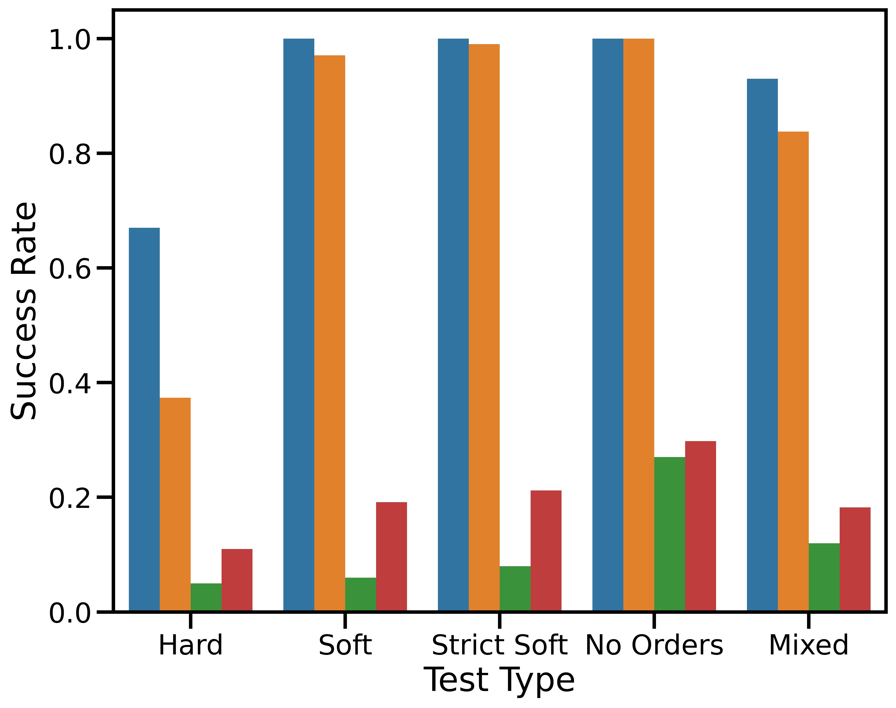
(a)

(b)

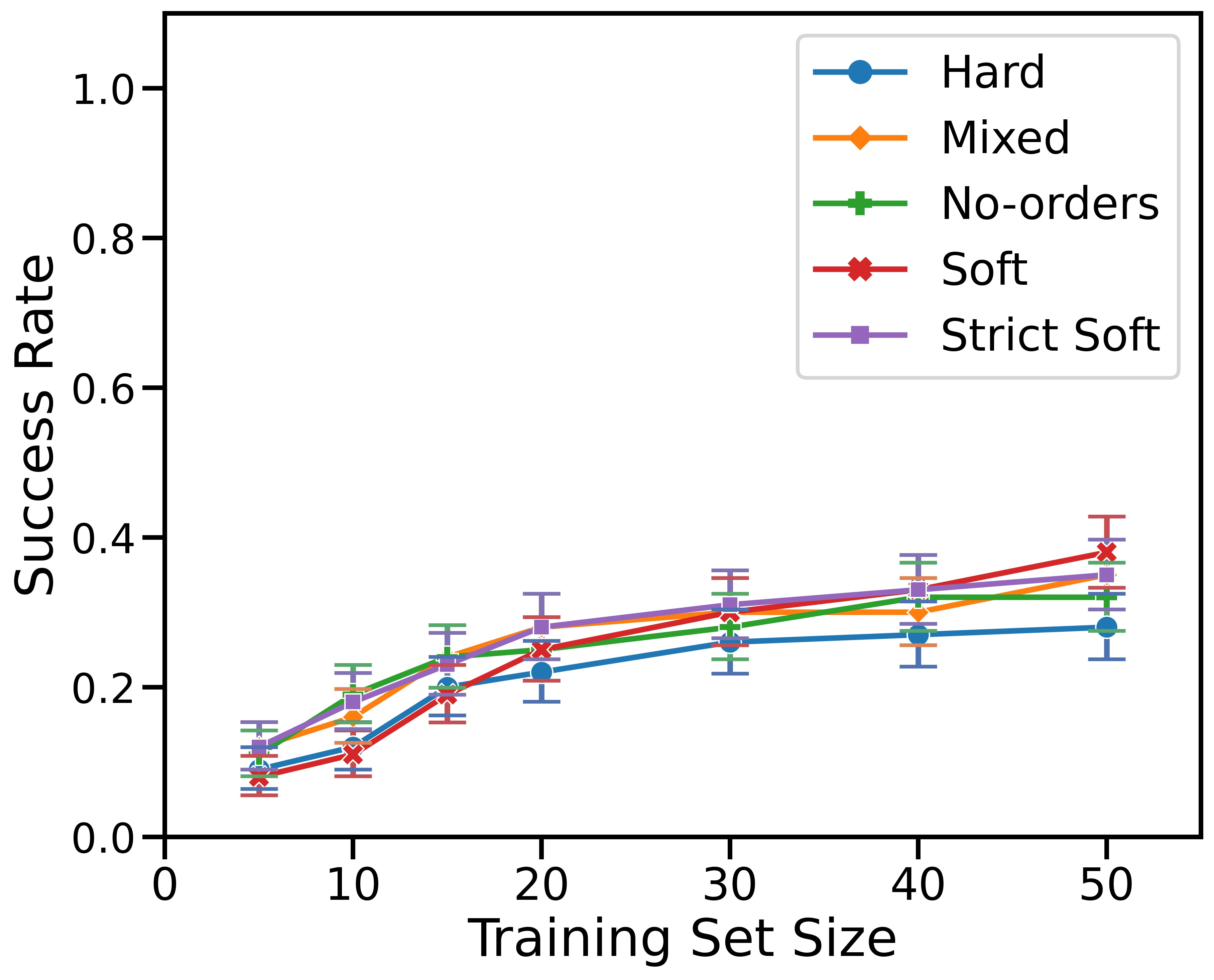
(c)

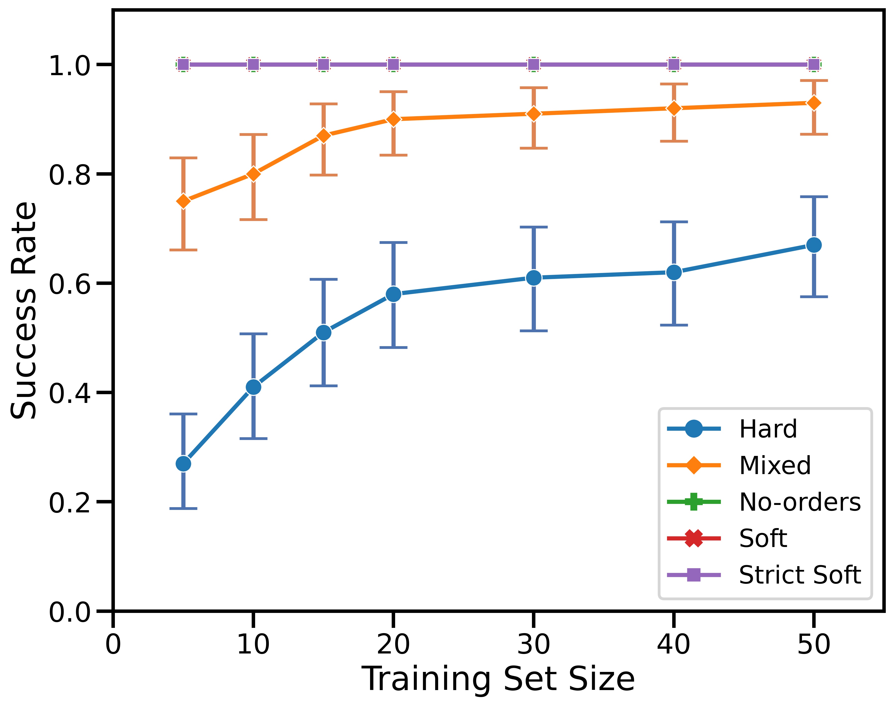
(d)

Figure 3: Figure 3(a) depicts the success rate on the mixed test set after training LTL-Transfer with Relaxed edge-matching criterion and three baselines on the mixed training set. Figure 3(b) shows the failure rate of each method. (Figures 3(a) and 3(b) share the legend.) Figure 3(c) depicts the success rate of the agent trained on mixed training sets of various sizes using LTL-Transfer with the Constrained edge-matching criterion when transferring to test sets of various specifications types. Figure 3(d) depicts the success rates with the Relaxed criterion. Note that the error bars depict the 95% credible interval if the successful transfer was modeled as a Bernoulli distribution.

VI-C Experiment configurations

All experiments were conducted on four different grid-world maps with a dimension of $19\times 19$. For each experimental run, we specified the training set type and size, and the test set type. The evaluation metrics include the success rate on each of the test set specifications. We logged the reason for any failed run.

The precomputations for compiling the set of transition-centric options were computed on a high-performance computing (HPC) cluster hosted by our university. As the compilation of state-centric options into transition-centric options allows for large-scale parallelism with no interdependency, we were able to share the workload among a large number of CPUs.

VII Results and Discussion

Comparison with Baselines We compare the performance of LTL-Transfer to three baselines, namely, LTL2Action [25], LPOPL [24], and a random action selection policy.

LTL2Action: Vaezipoor et al. [25] proposed embedding LTL specification through a graph neural network, and sequentially selecting the next proposition to turn true. This pre-trained embedding is then appended to the feature vector for the task policy yielding a goal-conditioned task policy. Vaezipoor et al. [25] termed the pre-trained policy as the LTL Bootcamp. We compare LTL-Transfer against LTL Bootcamp as that serves as the upper bound for performance of LTL2Action on novel task specifications. Note that our version of LTL Bootcamp is only trained on the same formulas included in the training task set of LTL-Transfer

LPOPL: LPOPL’s use of progressions and the multi-task learning framework allow it to handle tasks that lie within the progression set of the training formulas although it is not explicitly designed for zero-shot transfer. LPOPL’s limited capability of transferring to some novel specifications zero-shot serves as the lower bound that any transfer algorithm must surpass.

Random actions: To demonstrate the difficulty of the tasks due to the curse of history, we also compare our algorithm to a random action selection policy allowed to run for 500 time steps. Note that 500 steps is significantly larger than the usual number of actions required to complete the tasks.

Figure 3(a) depicts the success rate for the baselines and agent using LTL-Transfer when trained on a set of 50 specifications of the mixed training set. Each approach was tested on 100 new formulas in each of the test sets described in Section VI-B. LPOPL performed worse than the random action policy as it does not attempt to satisfy any task specification that does not exist in its progression set. Next, both LTL-Transfer and LTL2Action have near perfect success rate on soft, strictly soft, and no orders test set, as there are no irrecoverable failure for these specifications. Specification in hard and mixed test sets can fail irrecoverably, thus we observe a lower success rate across all transfer algorithms, however LTL-Transfer demonstrates the best transfer success rate in these difficult test sets. Crucially, LTL-Transfer never performed an action that resulted in an irrecoverable specification failure, while LTL2Action’s specification failure rate is very similar to the random action policy as shown in Figure 3(b).

Effect of edge matching criterion Next, we trained our agent on mixed specification types of varying sizes and used LTL-Transfer to transfer the learned policies to complete the specifications in all five test sets. The success rates with the Constrained edge matching criterion are depicted in Figure 3(c), while those for the Relaxed edge matching criterion are depicted in Figure 3(d). We note that the Relaxed edge matching criterion is capable of successfully transferring to a larger number of novel specifications across all specification types, thus supporting H1.

Relative difficulty of specification type Figure 3(c) indicates that the different specifications are equally difficult to transfer learned policies to when using the Constrained edge matching criterion. However, Figure 3(d) indicates that with the Relaxed edge matching criterion, LTL-Transfer is capable of transferring to novel specifications with soft, strictly soft order or no-orders after training on very few specifications. It also indicates that specifications with hard orders are the most difficult to transfer to. Therefore, H2 is supported only for the Relaxed edge matching criterion.

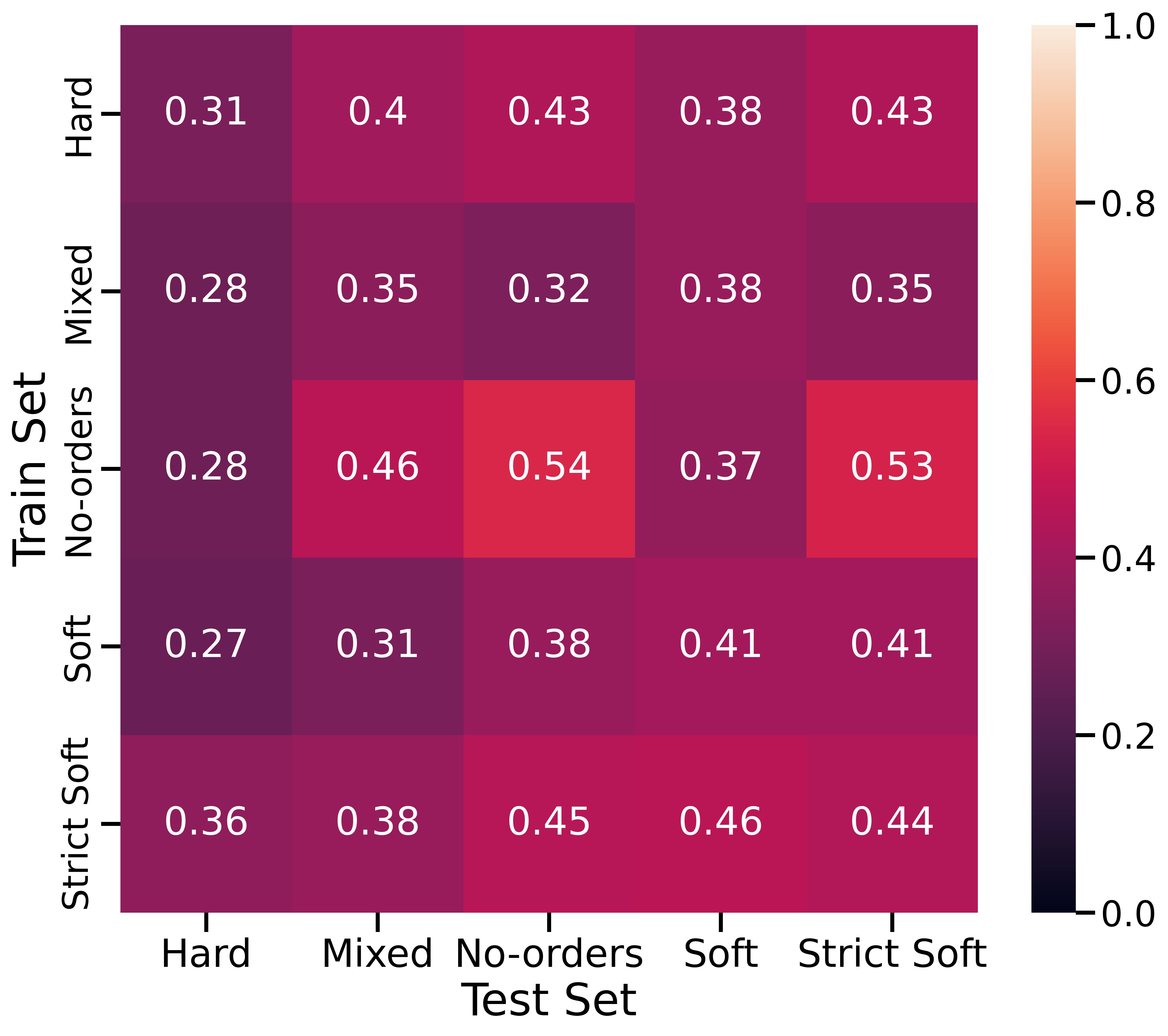
(a)

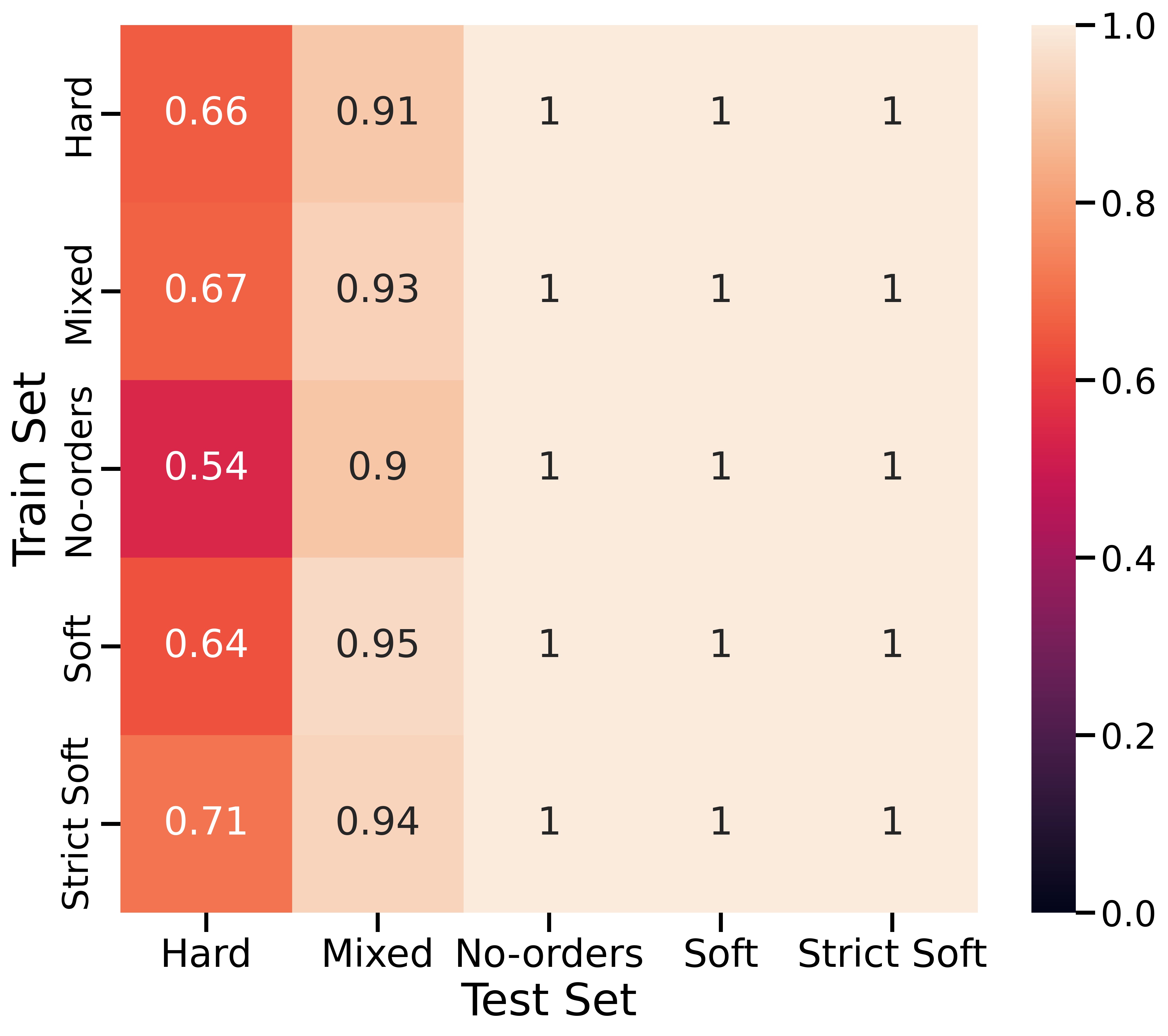
(b)

Figure 4: Figure 4(a) depicts the heatmap of success rates with various training and test specification types with the Constrained edge matching criterion. Similarly, Figure 4(b) depicts the heatmap with the Relaxed edge matching criterion.

Transferring across specification type Finally, we evaluate whether agents trained on different specification types are more capable of transferring to all other specification types. Figure 4(a) depicts the heatmap of success rates obtained by training the agent on 50 specifications of the type indicated by the row and transferring it to the test set of specification types indicated by the column while using the Constrained edge matching criterion. Similarly, Figure 4(b) depicts the success rates using the Relaxed edge matching criterion. No single specification type proved to be the best training set, thus providing evidence against H3. Further, training on all specification types leads to perfect transfer performance on soft, strictly-soft, and no-orders test set, thus providing further evidence for H2

We include the results of the complete set of experiments in Appendix A, and the selected trajectories from the test set in Appendix B.

VIII Robot Demonstrations

TABLE I: 10 Test LTL Tasks for Robot Demonstrations.

Test LTL Task	Expected to
$\mathbf{F}(book\wedge\mathbf{F}(desk_{a}\wedge\mathbf{F}(juice\wedge\mathbf{F}desk_{a})))$	succeed
$\mathbf{F}(book\wedge\mathbf{F}(desk_{a}\wedge\mathbf{F}(juice\wedge\mathbf{F}desk_{b})))$	succeed
$\mathbf{F}(book\wedge\mathbf{F}(desk_{b}\wedge\mathbf{F}(juice\wedge\mathbf{F}desk_{a})))$	succeed
$\mathbf{F}(book\wedge\mathbf{F}(desk_{b}\wedge\mathbf{F}(juice\wedge\mathbf{F}desk_{b})))$	succeed
$\mathbf{F}(juice\wedge\mathbf{F}(desk_{a}\wedge\mathbf{F}(book\wedge\mathbf{F}desk_{a})))$	succeed
$\mathbf{F}(juice\wedge\mathbf{F}(desk_{a}\wedge\mathbf{F}(book\wedge\mathbf{F}desk_{b})))$	succeed
$\mathbf{F}(juice\wedge\mathbf{F}(desk_{b}\wedge\mathbf{F}(book\wedge\mathbf{F}desk_{a})))$	succeed
$\mathbf{F}(juice\wedge\mathbf{F}(desk_{b}\wedge\mathbf{F}(book\wedge\mathbf{F}desk_{b})))$	succeed
$\neg desk_{a}~{}\mathbf{U}~{}book~{}\wedge~{}\neg juice~{}\mathbf{U}~{}desk_{a}~{}\wedge~{}\neg desk_{b}~{}\mathbf{U}~{}juice~{}\wedge~{}\mathbf{F}desk_{b}$	fail
$\neg desk_{b}~{}\mathbf{U}~{}juice~{}\wedge~{}\neg book~{}\mathbf{U}~{}desk_{b}~{}\wedge~{}\neg desk_{a}~{}\mathbf{U}~{}book~{}\wedge~{}\mathbf{F}desk_{a}$	fail

We deploy LTL-Transfer on Spot [5], a quadruped mobile manipulator, in an analog household environment where the robot can fetch and deliver objects while navigating through the space. LTL-Transfer first learned policies to solve two training tasks

$$\varPhi_{train}=\{ \mathbf{F}desk_{a}\wedge\neg desk_{a}~{}\mathbf{U}~{}book,$$

$$\mathbf{F}desk_{b}\wedge~{}\neg desk_{b}~{}\mathbf{U}~{}juice\}$$

in simulation, then transferred the learned skills to eight novel test tasks, as shown in Table I, in a zero-shot fashion. The robot can complete test tasks that it is expected to succeed, as shown in an example video . For novel tasks that LTL-Tansfer cannot solve because LTL-Transfer does not produce a feasible path through the reward machine graph given the transition-centric options learned from training tasks $\varPhi_{train}$, the robot aborts task execution as expected to avoid constraint violations.

We were limited by the lab space and used a testing environment of 25 grid cells. However, our algorithm can solve domains with much larger dimensions, like $19\times 19$ as presented in Section VI-C. The state space includes locations of the robot and four objects, i.e., two desks, a book on a bookshelf and a juice bottle on a kitchen counter. The robot moves in four cardinal directions, and an invalid action results in no movement. The robot performs the pick action after it moves to the grid cell containing $book$ or $juice$. We finetuned an off-the-shelf object detection model [29] to determine the grasp point from an RGB image by selecting the center point of the most confident bounding box. The robot performs the place action after it moves close to $desk_{a}$ or $desk_{b}$ while carrying an object. We use the built-in motion planners offered by the Spot’s Python API to move the robot base and gripper to specified poses.

IX Conclusion

We introduced LTL-Transfer, a novel algorithm that leverages the compositionality of linear temporal logic to solve a wide variety of novel LTL specifications. It segments policies from training tasks into portable, task-agnostic transition-centric options. We demonstrated that LTL-Transfer can solve over 90% of the 500 unseen task specifications in our Minecraft-inspired domains after training on only 50 specifications. We further demonstrated that LTL-Transfer never violated any safety constraints and aborted task execution when no feasible solution was found.

LTL-Transfer enables the possibility of maximally transferring the policies learned by the robot to new tasks. We envision further developing LTL-Transfer to incorporate long-term planning and intra-option policy updates to generate not just satisfying but optimal solutions to novel tasks.

Appendix

IX-A Additional Results

Cause of failure: As described in our draft, we logged the reason for failure for each unsuccessful transfer attempt as one of three possible causes: specification failure, where the agent violates a constraint and the reward machine is progressed to an unrecoverable state; no feasible path, where there are no matched transition-centric options for paths connecting the start state to an accepting state; options exhausted, where there are no further transition-centric options available to the agent to further progress the state of the task.

Figure 5 depicts the relative frequency of the failure modes when the agent is trained and tested on mixed task specifications. Note that with the Constrained edge-matching criterion, absence of feasible paths connecting the start and the accepting state is the primary reason for failure (Figure 5(a), whereas with the Relaxed edge-matching criterion, the agent utilizing all available safe options without progressing the task is the primary reason for failure (Figure 5(b)).

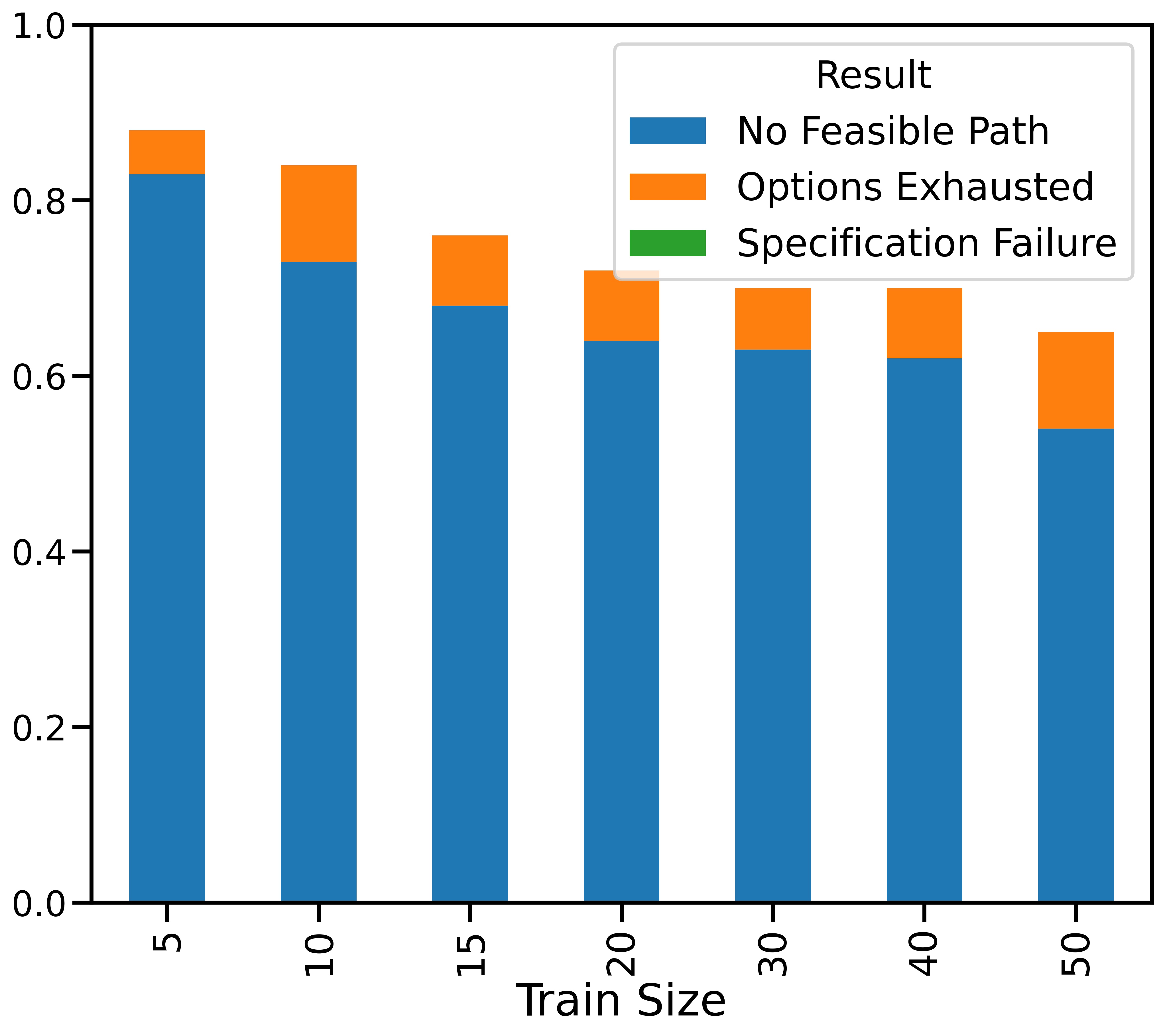
(a) Constrained

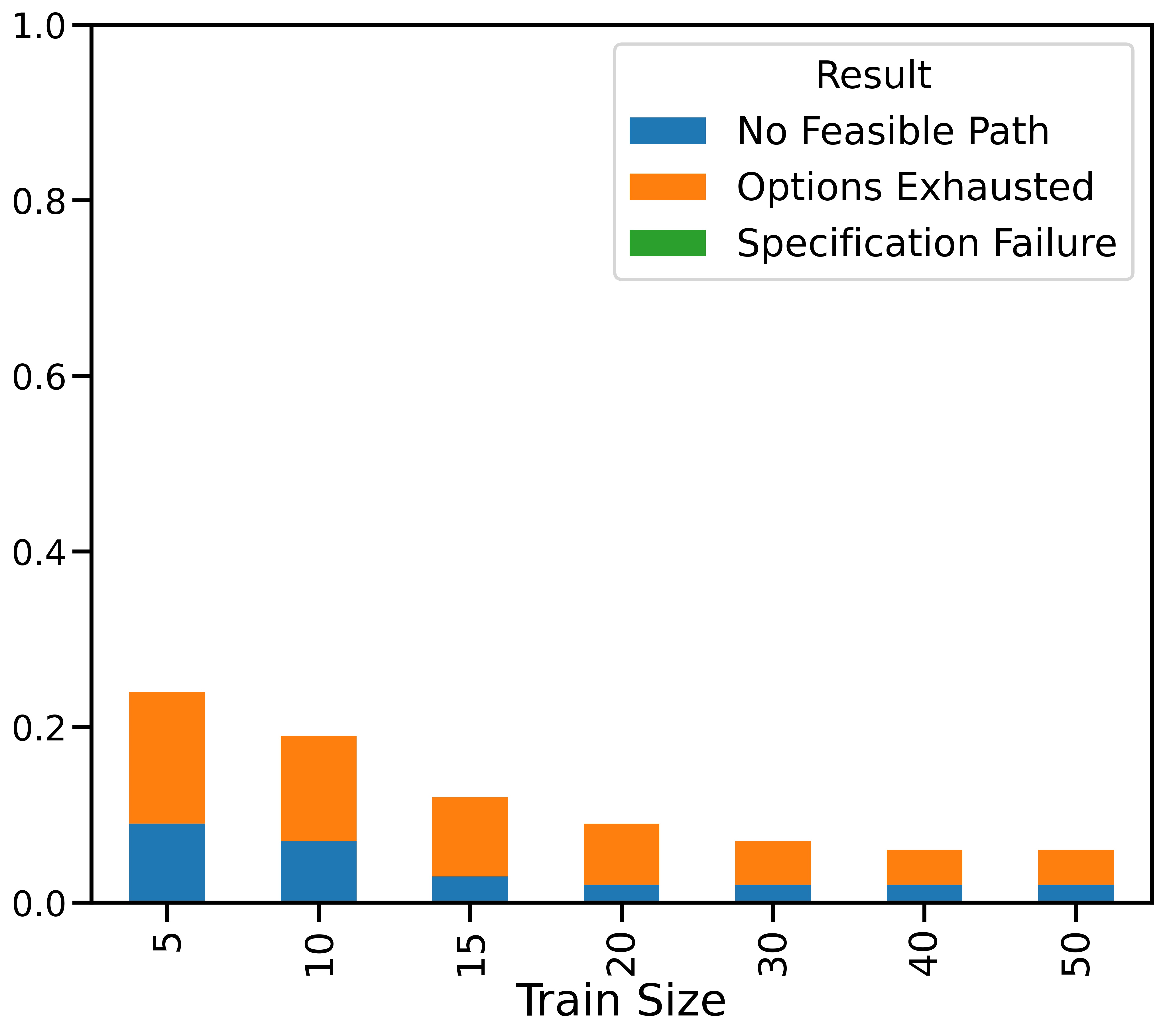
(b) Relaxed

Figure 5: Reasons for failed task executions for agents trained and evaluated on Mixed task specification datasets. Note that all values are depicted in fractions.

Learning curve for various training datasets: Next, we present the results for learning curve of the success rate when transferring policies learned on different specification types.

The learning curves for training on formulas from the Hard training set with both the edge matching criteria are depicted in Figure 6.

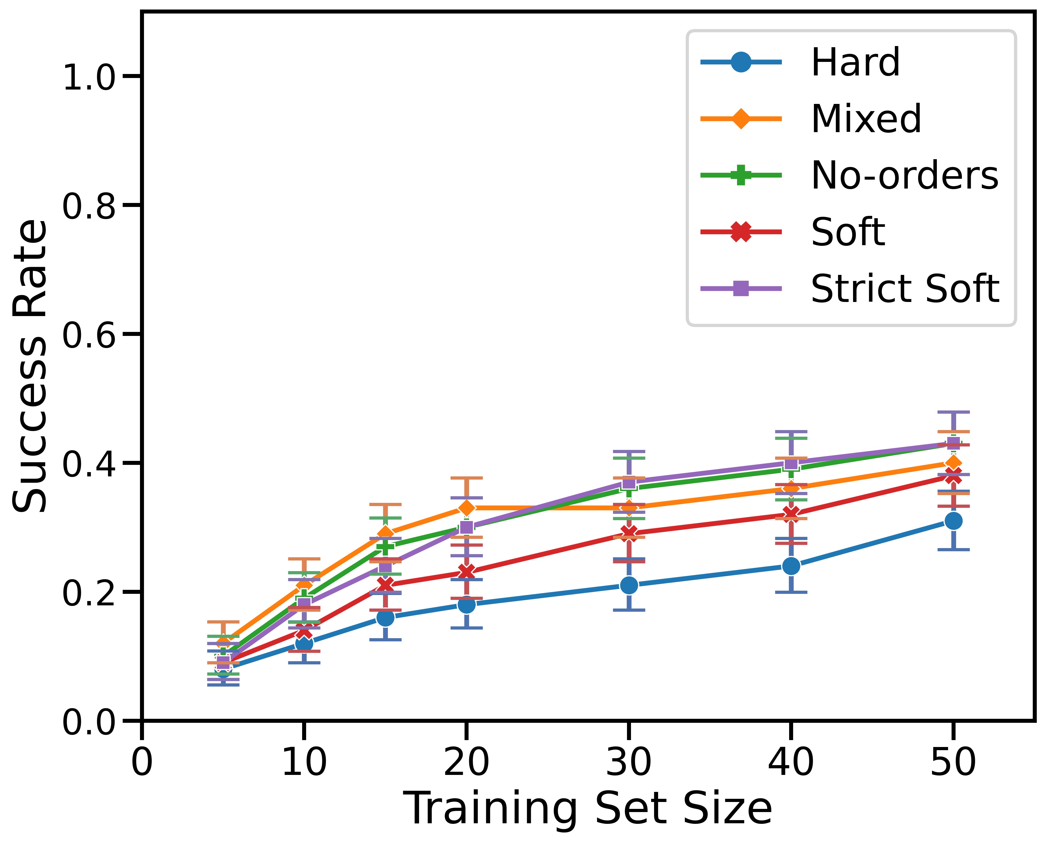
(a) Constrained

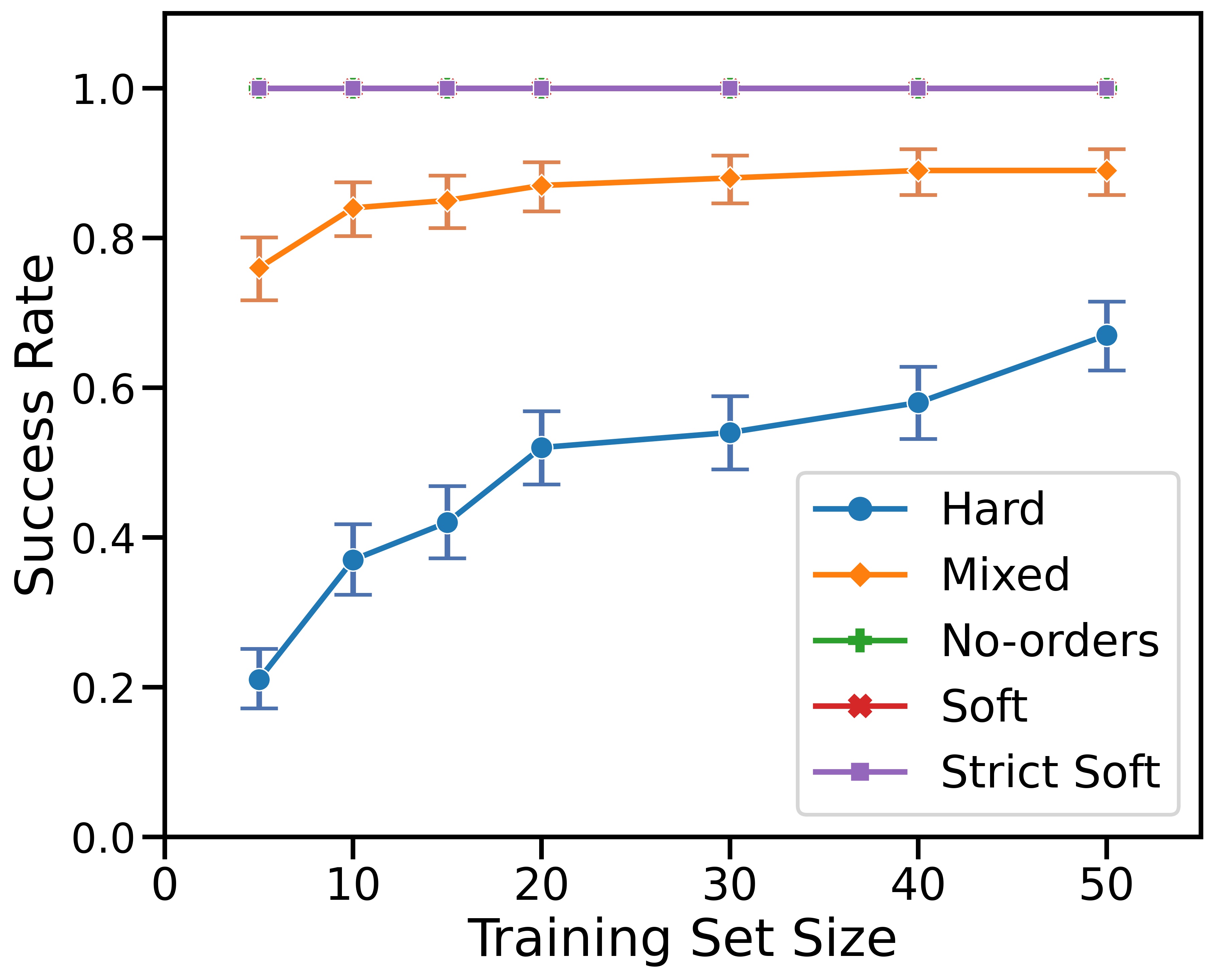
(b) Relaxed

Figure 6: Figure 6(a) depicts the success rate of the agent trained on Hard training sets of various sizes using LTL-Transfer with the constrained edge-matching criterion when transferring to test sets of various specifications types. Figure 6(b) depicts the success rates with the relaxed edge-matching criterion. Note that the error bars depict the 95% credible interval if the successful transfer was modeled as a Bernoulli distribution.

The learning curves for training on formulas from the Soft training set with both the edge matching criteria are depicted in Figure 7.

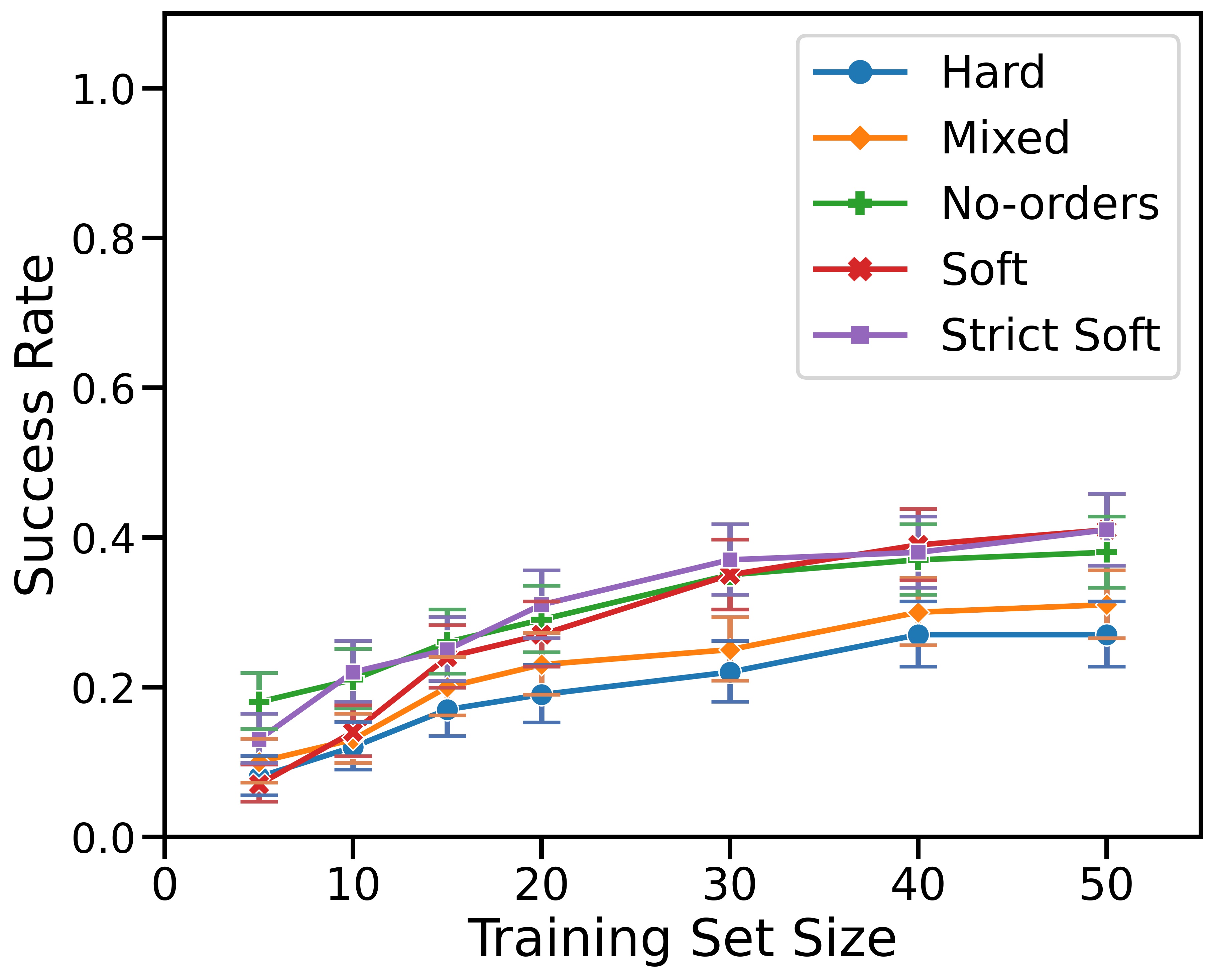
(a) Constrained

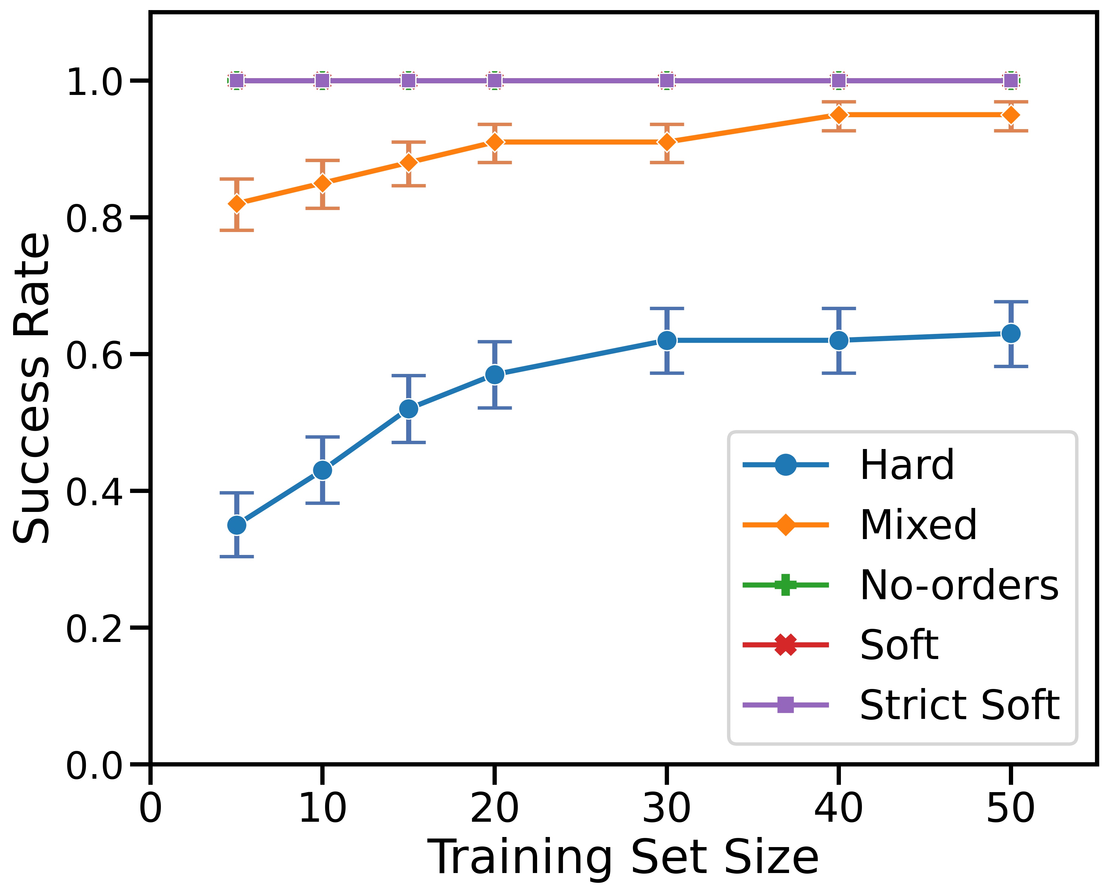
(b) Relaxed

Figure 7: Figure 7(a) depicts the success rate of the agent trained on Soft training sets of various sizes using LTL-Transfer with the constrained edge-matching criterion when transferring to test sets of various specifications types. Figure 7(b) depicts the success rates with the relaxed edge-matching criterion. Note that the error bars depict the 95% credible interval if the successful transfer was modeled as a Bernoulli distribution.

The learning curves for training on formulas from the Strictly Soft training set with both the edge matching criteria are depicted in Figure 8.

The learning curves for training on formulas from the No Orders training set are being generated at the time of submission, and are expected to share nearly identical trends as the learning curves from the other training sets given the completed data points. We will include the plots in the final version of the paper.

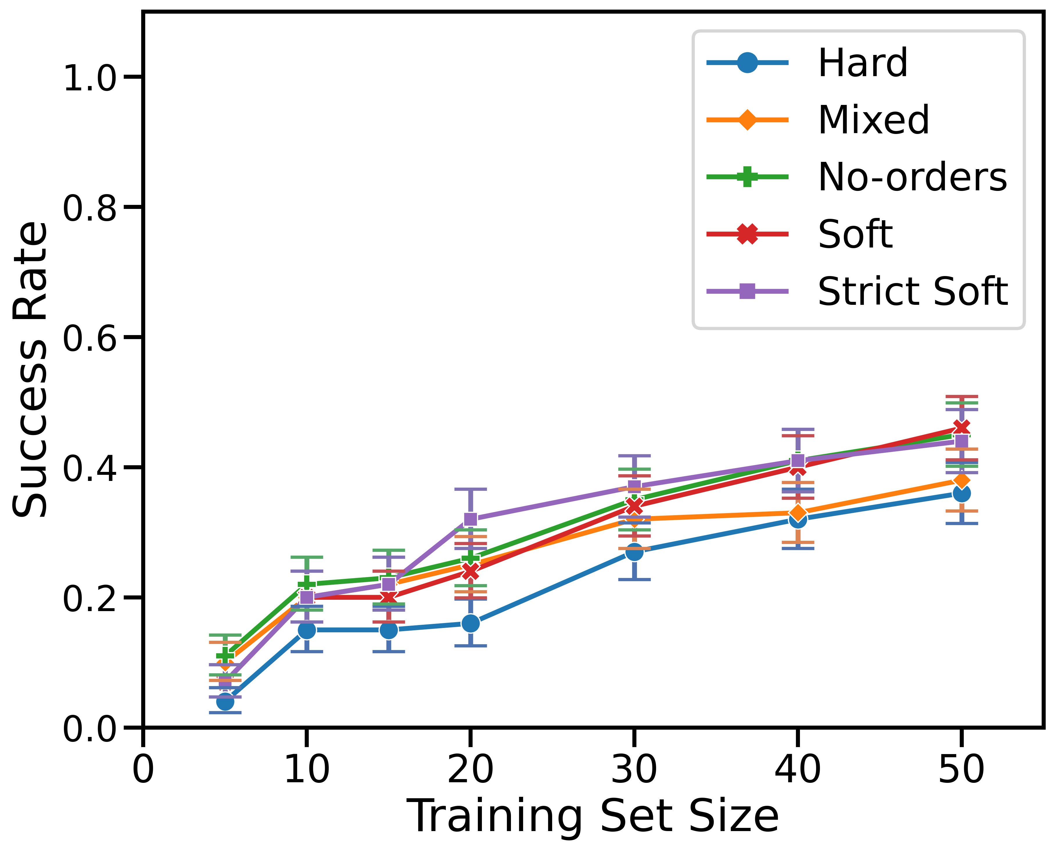
(a) Constrained

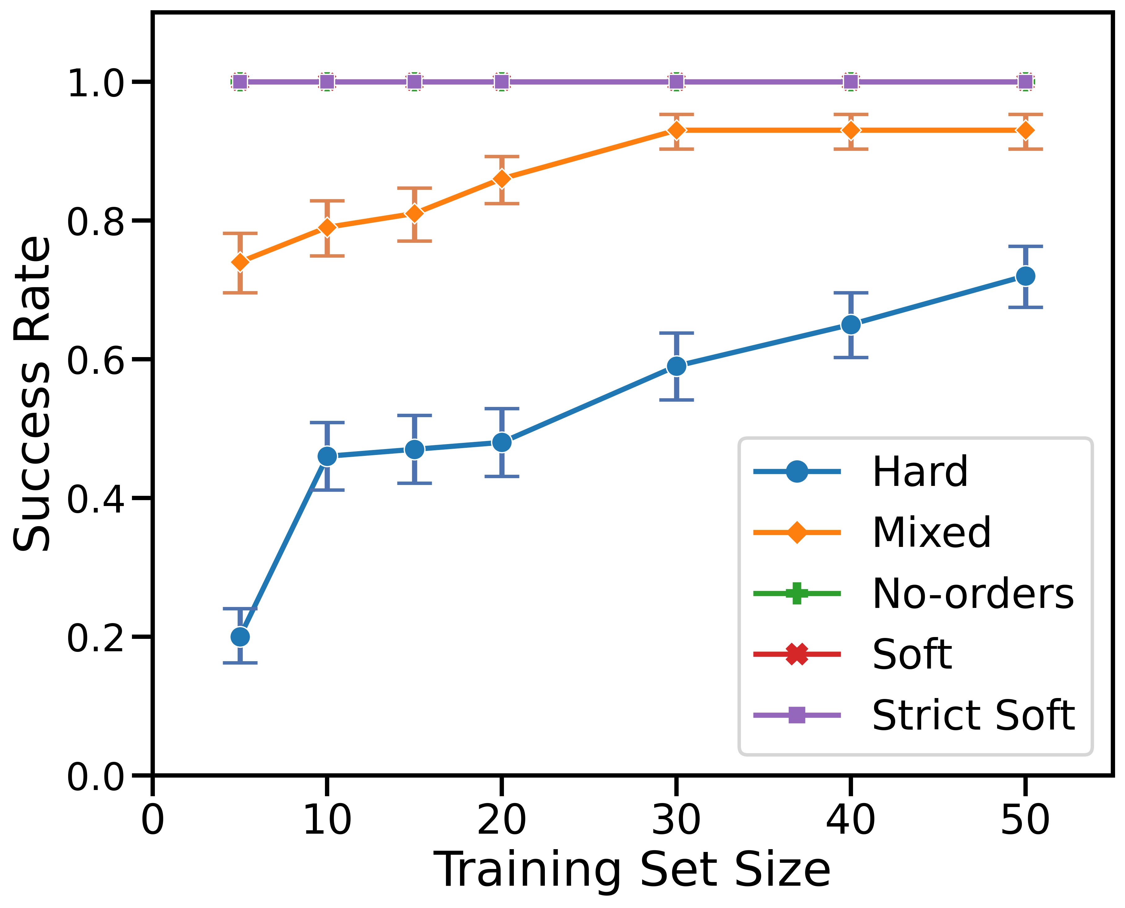
(b) Relaxed

Figure 8: Figure 8(a) depicts the success rate of the agent trained on Strictly Soft training sets of various sizes using LTL-Transfer with the constrained edge-matching criterion when transferring to test sets of various specifications types. Figure 8(b) depicts the success rates with the relaxed edge-matching criterion. Note that the error bars depict the 95% credible interval if the successful transfer was modeled as a Bernoulli distribution.

Note that for training on each of the specification types, the learning curve trends are nearly identical to the learning curves on training with Mixed specification types as depicted in Figure 3 in the main draft. Hard specification types remain the most challenging specification ordering types to transfer to.

IX-B Selected Solution Trajectories

Consider the case with mixed training set with $5$ formulas on map 0. The training formulas are:

• $\mathbf{F}grass~{}\wedge~{}\mathbf{F}shelter~{}\wedge~{}\mathbf{F}(wood~{}\wedge~{}\mathbf{X}\mathbf{F}workbench)$

• $\mathbf{F}toolshed~{}\wedge~{}\mathbf{F}workbench~{}\wedge~{}\mathbf{F}shelter~{}\wedge~{}\\ (\neg toolshed~{}\mathbf{U}~{}shelter)~{}\wedge~{}\mathbf{F}(grass~{}\wedge~{}\mathbf{F}bridge)$

• $\mathbf{F}toolshed~{}\wedge~{}\mathbf{F}(shelter~{}\wedge~{}\mathbf{F}(axe~{}\wedge~{}\mathbf{F}wood))$

• $\mathbf{F}iron~{}\wedge~{}\mathbf{F}(shelter~{}\wedge~{}\mathbf{X}\mathbf{F}(bridge~{}\wedge~{}\mathbf{X}\mathbf{F}factory))$

• $\mathbf{F}factory$

One of the Mixed test formulas was $\varphi_{test}=\mathbf{F}workbench~{}\wedge~{}\mathbf{F}grass~{}\wedge~{}\mathbf{F}axe$. The reward machine for this task specification is depicted in Figure 9(a). Given the training set of formulas, and the use of the Constrained edge matching criterion, the start state is disconnected from all downstream states as no transition-centric options match with the edge transitions. Therefore, the agent does not attempt to solve the task and returns failure with the reason being no feasible path, i.e., a disconnected reward machine graph after removing infeasible edges.

If the Relaxed edge matching criterion is used, there are matching transition-centric options for each of the RM edges. The trajectory adopted by the agent when transferring the policies is depicted in Figure 10. The agent collects all the three requisite resources before it terminates the task execution. Further note that the agent passes through a $wood$ resource grid as the specification does not explicitly prohibit it.

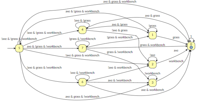
(a)

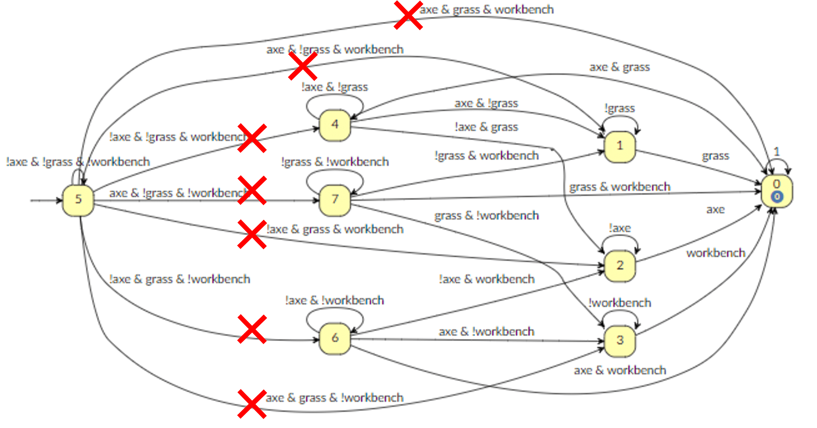
(b)

Figure 9: Figure 9(a) depicts the reward machine for the the specification $\varphi_{test}=\mathbf{F}workbench~{}\wedge~{}\mathbf{F}grass~{}\wedge~{}\mathbf{F}axe$, as well as all feasible edges matched by the Relaxed criterion. Note that all the edges have at least one matched transition-centric option for the Relaxed criterion. Figure 9(b) depicts the edges that do not have a compatible transition-centric option for the Constrained edge matching criterion.

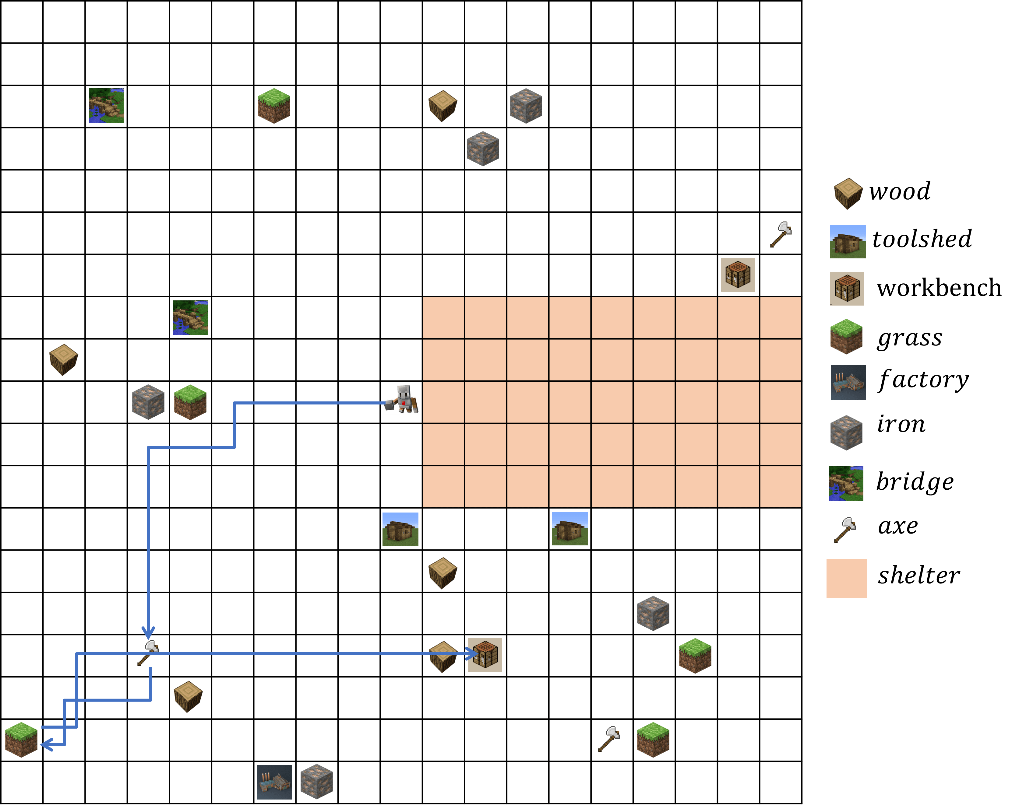
Figure 10: Trajectory executed by the agent using LTL-Transfer on the specification $\varphi_{test}=\mathbf{F}workbench~{}\wedge~{}\mathbf{F}grass~{}\wedge~{}\mathbf{F}axe$.

IX-C Example specifications

Here we provide the specifications and the interpretations of three formulas each from the Hard, Soft, Strictly Soft, No Orders, and Mixed formula types. Note that the training set contained 50 formulas each (new formulas were added incrementally when varying the training set size), and the test set contained 100 formulas each.

Hard: Example formulas belonging to the Hard dataset are as follows:

1. $\mathbf{F}wood~{}\wedge~{}\mathbf{F}axe~{}\wedge\neg wood~{}\mathbf{U}~{}grass~{}\wedge~{}\\ \neg grass~{}\mathbf{U}~{}workbench~{}\wedge~{}\neg workbench~{}\mathbf{U}~{}bridge$: Visit $bridge$, $workbench$, $grass$, $wood$, and $axe$. Ensure that $bridge$, $workbench$, $grass$, $wood$ in that particular order. Objects later in the sequence cannot be visited before the prior objects.

2. $\mathbf{F}workbench~{}\wedge\mathbf{F}factory~{}\wedge~{}\mathbf{F}iron~{}\wedge~{}\mathbf{F}shelter~{}\wedge\\ ~{}\neg factory~{}\mathbf{U}~{}axe$: Visit $workbench$, $factory$, $iron$, $shelter$, and $axe$. Ensure that $factory$ is not visited before $axe$.

3. $\mathbf{F}toolshed~{}\wedge~{}\mathbf{F}bridge~{}\wedge~{}\mathbf{F}factory~{}\wedge~{}\mathbf{F}axe~{}\wedge\\ ~{}\neg bridge~{}\mathbf{U}~{}wood$: Visit $toolshed$, $bridge$, $factory$, $axe$, and $wood$. Ensure that $bridge$ is not visited before $wood$.

Soft: Examples belonging to the Soft dataset are as follows:

1. $\mathbf{F}(bridge~{}\wedge~{}\mathbf{F}(factory~{}\wedge~{}\mathbf{F}(iron~{}\wedge~{}\mathbf{F}shelter)))$: Visit $bridge$, $factory$, $iron$, and $shelter$ in that sequence. The objects later in the sequence may be visited before the prior objects, provided that they are visited at least once after the prior object has been visited.

2. $\mathbf{F}workbench~{}\wedge\mathbf{F}(factory~{}\wedge~{}\mathbf{F}grass)$: Visit the $workbench$, $factory$, and $grass$: Visit $grass$ at least once after visiting the $factory$.

3. $\mathbf{F}(axe~{}\wedge~{}\mathbf{F}factory)~{}\wedge\mathbf{F}workbench$: Visit $axe$, $factory$, and $workbench$. Ensure that $factory$ is visited at least once after $axe$ is.

Strictly Soft: Examples belonging to the Strictly Soft dataset are identical to the Soft specifications, except they do not allow for simultaneous satisfaction of multiple sub-tasks. The subtasks in sequence must occur strictly temporally after the prior subtask. This is enforced using $\mathbf{X}\mathbf{F}a$ instead of $\mathbf{F}a$.

No Orders: These specifications only contain a list of subtasks to be completed. No temporal orders are enforced between the various subtasks.

Mixed: Examples belonging to the Mixed dataset are as follows:

1. $\mathbf{F}toolshed~{}\wedge\mathbf{F}factory~{}\wedge\neg toolshed~{}\mathbf{U}~{}shelter~{}\wedge\mathbf{F}(grass~{}\wedge~{}\mathbf{F}bridge)$: Visit the $toolshed$, $factory$, $shelter$, $grass$, and $bridge$. Ensure that $toolshed$ is not visited before the shelter, and $bridge$ is visited at least once after $grass$.

2. $\mathbf{F}grass~{}\wedge~{}\neg grass~{}\mathbf{U}~{}toolshed~{}\wedge~{}\\ \mathbf{F}(factory~{}\wedge~{}\mathbf{X}\mathbf{F}workbench)$: Visit $grass$, $toolshed$, $factory$, and $workbench$. Ensure that $grass$ is not visited before $toolshed$, and $workbench$ is at least visited once strictly after $factory$.

3. $\mathbf{F}iron~{}\wedge~{}\neg iron~{}\mathbf{U}~{}toolshed~{}\wedge~{}\mathbf{F}(shelter~{}\wedge~{}\mathbf{X}\mathbf{F}wood)$: Visit $iron$, $toolshed$, $shelter$, and $wood$. Ensure that $iron$ is not visited before $toolshed$, and $wood$ is at least visited once strictly after $shelter$.

References

- Andreas et al. [2017] Jacob Andreas, Dan Klein, and Sergey Levine. Modular multitask reinforcement learning with policy sketches. In International Conference on Machine Learning, pages 166–175. PMLR, 2017.
- Araki et al. [2021] Brandon Araki, Xiao Li, Kiran Vodrahalli, Jonathan Decastro, Micah Fry, and Daniela Rus. The logical options framework. In Marina Meila and Tong Zhang, editors, Proceedings of the 38th International Conference on Machine Learning, volume 139 of Proceedings of Machine Learning Research, pages 307–317. PMLR, 18–24 Jul 2021. URL https://proceedings.mlr.press/v139/araki21a.html.
- Bagaria and Konidaris [2019] Akhil Bagaria and George Konidaris. Option discovery using deep skill chaining. In International Conference on Learning Representations, 2019.
- Bagaria et al. [2021] Akhil Bagaria, Jason Senthil, Matthew Slivinski, and George Konidaris. Robustly learning composable options in deep reinforcement learning. In Proceedings of the 30th International Joint Conference on Artificial Intelligence, 2021.
- [5] Boston Dynamics. Spot® - the agile mobile robot. https://www.bostondynamics.com/products/spot.
- Camacho et al. [2019] Alberto Camacho, Rodrigo Toro Icarte, Toryn Q Klassen, Richard Anthony Valenzano, and Sheila A McIlraith. Ltl and beyond: Formal languages for reward function specification in reinforcement learning. In IJCAI, volume 19, pages 6065–6073, 2019.
- Gerth et al. [1995] Rob Gerth, Doron Peled, Moshe Y Vardi, and Pierre Wolper. Simple on-the-fly automatic verification of linear temporal logic. In International Conference on Protocol Specification, Testing and Verification, pages 3–18. Springer, 1995.
- Icarte et al. [2018] Rodrigo Toro Icarte, Toryn Klassen, Richard Valenzano, and Sheila McIlraith. Using reward machines for high-level task specification and decomposition in reinforcement learning. In International Conference on Machine Learning, pages 2107–2116. PMLR, 2018.
- Icarte et al. [2022] Rodrigo Toro Icarte, Toryn Q Klassen, Richard Valenzano, and Sheila A McIlraith. Reward machines: Exploiting reward function structure in reinforcement learning. Journal of Artificial Intelligence Research, 73:173–208, 2022.
- James et al. [2020] Steven James, Benjamin Rosman, and George Konidaris. Learning portable representations for high-level planning. In International Conference on Machine Learning, pages 4682–4691. PMLR, 2020.
- Jothimurugan et al. [2021] Kishor Jothimurugan, Suguman Bansal, Osbert Bastani, and Rajeev Alur. Compositional reinforcement learning from logical specifications. In Thirty-Fifth Conference on Neural Information Processing Systems, 2021.
- Konidaris and Barto [2007] George Dimitri Konidaris and Andrew G Barto. Building portable options: Skill transfer in reinforcement learning. In IJCAI, volume 7, pages 895–900, 2007.
- Kuo et al. [2020] Yen-Ling Kuo, Boris Katz, and Andrei Barbu. Encoding formulas as deep networks: Reinforcement learning for zero-shot execution of ltl formulas. In 2020 IEEE/RSJ International Conference on Intelligent Robots and Systems (IROS), pages 5604–5610. IEEE, 2020.
- Kupferman and Vardi [2001] Orna Kupferman and Moshe Y Vardi. Model checking of safety properties. Formal methods in system design, 19(3):291–314, 2001.
- León et al. [2022a] Borja G León, Murray Shanahan, and Francesco Belardinelli. Systematic generalisation through task temporal logic and deep reinforcement learning. Adaptive and Learning Agents Workshop at International Conference on Autonomous Agents and Multiagent Systems, 2022a.
- León et al. [2022b] Borja G León, Murray Shanahan, and Francesco Belardinelli. In a nutshell, the human asked for this: Latent goals for following temporal specifications. In International Conference on Learning Representations (ICLR), 2022b.
- Littman et al. [2017] Michael L Littman, Ufuk Topcu, Jie Fu, Charles Isbell, Min Wen, and James MacGlashan. Environment-independent task specifications via gltl. arXiv preprint arXiv:1704.04341, 2017.
- Manna and Pneuli [1990] Zohar Manna and Amir Pneuli. A hierarchy of temporal properties. In ACM symposium on Principles of distributed computing, 1990.
- Patel et al. [2020] Roma Patel, Ellie Pavlick, and Stefanie Tellex. Grounding language to non-markovian tasks with no supervision of task specifications. In Robotics: Science and Systems, 2020.
- Pnueli [1977] Amir Pnueli. The temporal logic of programs. In 18th Annual Symposium on Foundations of Computer Science (sfcs 1977), pages 46–57. ieee, 1977.
- Shah et al. [2018] Ankit Shah, Pritish Kamath, Julie A Shah, and Shen Li. Bayesian inference of temporal task specifications from demonstrations. Advances in Neural Information Processing Systems, 31, 2018.
- Sutton et al. [1999] Richard S. Sutton, Doina Precup, and Satinder Singh. Between mdps and semi-mdps: A framework for temporal abstraction in reinforcement learning. Artificial Intelligence, 112(1):181–211, 1999. ISSN 0004-3702. doi: https://doi.org/10.1016/S0004-3702(99)00052-1. URL https://www.sciencedirect.com/science/article/pii/S0004370299000521.
- Taylor et al. [2009] M.E. Taylor, , and P. Stone. Transfer learning for reinforcement learning domains: A survey. Journal of Machine Learning Research, 10(Jul):1633–1685, 2009.
- Toro Icarte et al. [2018] Rodrigo Toro Icarte, Toryn Q. Klassen, Richard Valenzano, and Sheila A. McIlraith. Teaching multiple tasks to an RL agent using LTL. In Proceedings of the 17th International Conference on Autonomous Agents and MultiAgent Systems (AAMAS), pages 452–461, 2018.
- Vaezipoor et al. [2021] Pashootan Vaezipoor, Andrew C Li, Rodrigo A Toro Icarte, and Sheila A Mcilraith. LTL2action: Generalizing LTL instructions for multi-task RL. In International Conference on Machine Learning, pages 10497–10508. PMLR, 2021.
- Valiant [1979] Leslie G Valiant. The complexity of computing the permanent. Theoretical computer science, 8(2):189–201, 1979.
- Vardi [1996] Moshe Y Vardi. An automata-theoretic approach to linear temporal logic. Logics for concurrency, pages 238–266, 1996.
- Xu and Topcu [2019] Zhe Xu and Ufuk Topcu. Transfer of temporal logic formulas in reinforcement learning. In IJCAI: proceedings of the conference, volume 28, page 4010. NIH Public Access, 2019.
- Yu et al. [2020] Hongkun Yu, Chen Chen, Xianzhi Du, Yeqing Li, Abdullah Rashwan, Le Hou, Pengchong Jin, Fan Yang, Frederick Liu, Jaeyoun Kim, and Jing Li. TensorFlow Model Garden. https://github.com/tensorflow/models, 2020.