Model-based machine learning of critical brain dynamics

Abstract

Criticality can be exactly demonstrated in certain models of brain activity, yet it remains challenging to identify in empirical data. We trained a fully connected deep neural network to learn the phases of an excitable model unfolding on the anatomical connectome of human brain. This network was then applied to brain-wide fMRI data acquired during the descent from wakefulness to deep sleep. We report high correlation between the predicted proximity to the critical point and the exponents of cluster size distributions, indicative of subcritical dynamics. This result demonstrates that conceptual models can be leveraged to identify the dynamical regime of real neural systems.

The criticality hypothesis states that neural activity is posed at or near the critical point of a second order phase transition Chialvo (2010); Cocchi et al. (2017). Theoretical support for this hypothesis is found in the information processing benefits that result from operating near the critical point, such as increased dynamic range, capacity for information transmission, and information capacity Kinouchi and Copelli (2006); Shew and Plenz (2013); Beggs (2008). At the critical point, the repertoire of possible states is maximized, together with the susceptibility and correlation length Haimovici et al. (2013); Expert et al. (2011); Hahn et al. (2017). In combination, these properties result in highly differentiated dynamics, yet also integrated and reactive, as considered necessary to support higher cognitive function and conscious awareness Tononi (2004); Mashour et al. (2020).

Although criticality presents distinct signatures, establishing it from neural activity recordings remains challenging Beggs and Timme (2012). Experiments using an ample variety of recording techniques have found evidence of scale-free neural activity avalanches, a landmark feature of self-organized criticality Bak et al. (1988); Beggs and Plenz (2003); Priesemann et al. (2014); Tagliazucchi et al. (2012); Shriki et al. (2013); Scott et al. (2014). However, it is difficult to demonstrate power law relationships with a limited amount of noisy data; moreover, there are other mechanisms consistent with scale-free behavior besides criticality Girardi-Schappo (2021). Other possible signatures of criticality are based on branching ratios Poil et al. (2008), spatio-temporal correlations Expert et al. (2011); Haimovici et al. (2013), and the response to external perturbations Tagliazucchi et al. (2016). While these alternative metrics have been explored with success, establishing a single unified criterion for the presence of criticality in neural systems remains an open problem.

In contrast to experimental data, criticality can be rigorously demonstrated in mathematical models of physical systems, including some models used to represent neural activity, such as those based on self-organized criticality Bak et al. (1988). Even in models lacking neurobiological realism, the universality of dynamics near criticality could ensure the statistical similarity between real and simulated activity Chialvo (2010); Cocchi et al. (2017). We explored this idea by implementing a model known to exhibit a second order phase transition (Greenberg-Hastings cellular automata) Haimovici et al. (2013) coupled with the anatomical connectome, obtained using diffusion spectrum imaging (DSI) Hagmann et al. (2008). We trained a deep neural network to output the probability of the model operating at the sub- and supercritical regimes, which allowed us to correctly identify the critical point as the crossing point between both probabilities. Next, we showed that the probabilities obtained from the neural network applied to empirical functional magnetic resonance imaging (fMRI) data presented high correlation with the power-law exponents of avalanche distributions obtained from the same data across different brain states (wakefulness and all stages of the human non-rapid eye movement [NREM] sleep cycle). Thus, we showed that the proximity to critical dynamics can be estimated from multivariate experimental data by means of a machine learning algorithm trained using simulations of a conceptual model of brain activity exhibiting criticality.

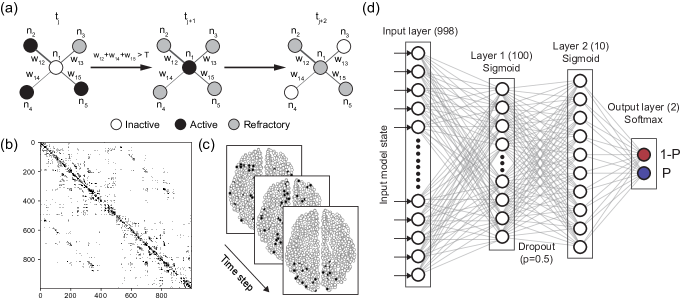
Figure 1: Methodological overview. (a) Transition rules for the local dynamics in the Greenberg-Hastings model, where $t_{i}$ is the $i$-th discrete time step, $n_{i}$ is the $i$-th node, $W_{ij}$ is the connection weight between nodes $i,j$, and $T$ is the threshold for the propagation of activity. (b) Matrix representation of the anatomical connectome used in the model, corresponding to 998 nodes densely connected by weights estimated using DSI. (c) Example of the model output evolving over time. (d) Diagram of the neural network architecture used to learn the proximity to criticality in the model, consisting of one input layer (998 units, one per node in the model), followed by two internal layers (100 and 10 units, respectively) with sigmoid activation functions, densely connected with 0.5 dropout probability, and by an output layer with two softmax units.

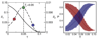
Figure 2: Learning the phase transition. Left: Phase transition in the model (adapted from Haimovici et al. (2013)). Here $S_{1}$ and $S_{2}$ stand for the largest and second largest connected clusters of active nodes. The red, blue and green dots indicate sub-, super-, and critical points of the model, with the critical threshold $T_{c}\approx 0.05$. Right: Probability of sub- and supercritical dynamics (red and blue, respectively; mean $\pm$ S.D.), obtained from applying the neural network to the independent holdout set. The crossing of both plots at $P=0.05$ indicates the critical point, matching the expected value of $T_{c}\approx 0.05$.

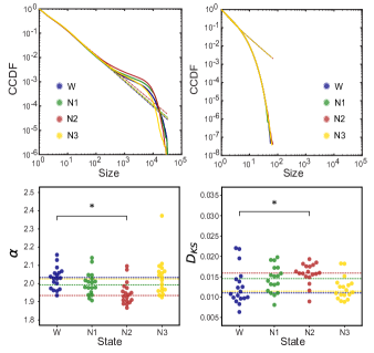
Figure 3: Scale-free dynamics in fMRI data. Upper left: complementary cumulative distribution functions (CCDF) for the size of connected clusters of active voxels obtained for wakefulness (W), and sleep (N1, N2, N3). Dotted lines correspond to power laws with exponents obtained using a maximum likelihood estimator applied to the empirical distributions. Upper right: same but obtained after randomly shuffling the phases of the voxel-wise signals. Lower left: swarm plots of the Fisher exponents $\alpha$ estimated for each participant and sleep stage (*p$<$0.05, Wilcoxon signed-rank test). Lower right: swarm plots of the goodness of fit, estimated as the Kolmogorov-Smirnov distance ($D_{KS}$) between the empirical distributions and the optimal fits (*p$<$0.05, Wilcoxon signed-rank test). All p-values were Bonferroni corrected for all pairwise comparisons between wakefulness and sleep states.

Brain activity model.— We consider the Greenberg-Hastings model of excitable dynamics. The possible states and transition rules are shown in Fig. 1a. An inactive node $n_{i}$ can become active spontaneously with a small probability ($10^{-3}$), or if sum of the connection weights with its neighbouring active nodes is larger than a threshold, $\sum_{j}a_{j}W_{ij}>T$ where $a_{j}=1$ if $n_{j}$ is active and 0 otherwise. After becoming active, a node transition towards refractory in the next time step. For each time step, refractory node has a probability of $10^{-1}$ of returning to the inactive state. The model consists of 998 nodes connected according to the matrix $W_{ij}$ shown in Fig. 1b, obtained using DSI by Hagmann et al Hagmann et al. (2008). The output of the model is a time series of binary (1 if active, 0 otherwise) vectors, representing the temporal evolution of the activations (Fig. 1c).

Learning the phase transition.— We implemented a fully connected deep neural network with an architecture illustrated in Fig. 1d. The input layer received the configuration of active nodes at each time step. This was followed by two hidden layers with 100 and 10 units, respectively, both with sigmoid activation functions, and by two softmax units in the output layer. The network was trained using L2 regularization with parameter equal to 0.01. To avoid overfitting, the connection between the hidden layers had a dropout rate of 0.5.

This network was trained using examples simulated with the model using different $T$ values. Without spontaneous excitation, the Greenberg-Hastings model presents a phase transition at the point where activity becomes self-sustained Fisch et al. (1993). As shown by Haimovici et al. and depicted in Fig. 2 (left), in the model with spontaneous excitation the phase transition can be described using $S_{1}$ (the size of the largest connected cluster) as order parameter, with $S_{2}$ peaking at the transition point (for this choice of $W_{ij}$ the critical value is $T_{c}\approx 0.05$) Haimovici et al. (2013).

To train the network, we simulated the model with $T$ ranging from 0.01 to 0.1 with step 0.001, starting from a configuration with 100 randomly active nodes and discarding the first 300 time steps to avoid transitory effects. For each $T$ value we simulated 1000 independent realizations, using 60% of these to train the network and 40% as a holdout set for evaluation. The network was trained to predict the phase, with $y_{1}$,$y_{2}$ the target value of the two output units and $y_{1}=1,y_{2}=0$ if $T<T_{c}$, $y_{1}=0,y_{2}=1$ otherwise, using backpropagation with the Adam optimizer with 10 training epochs, and loss function given by the categorical cross-entropy, $-y_{1}log(\hat{y}_{1})-y_{2}log(\hat{y}_{2})$ ($\hat{y}_{1},\hat{y}_{2}$ are the values of the two output units). As shown in Fig. 2 (right) the neural network is capable of predicting the critical point (crossing of both probabilities at $\approx$ 0.05) in the independent holdout set.

Power-law exponents in fMRI data.— We thresholded each brain voxel in fMRI data with a threshold of +1 S.D. and obtained the distribution of sizes of activated clusters, $p(s)$ Tagliazucchi et al. (2012). As shown in previous work Tagliazucchi et al. (2012); Bocaccio et al. (2019), this distribution follows a power law $p(s)\propto s^{-\alpha}$, with $\alpha\approx 2$ (Fisher exponent Fisher (1967)). We performed this analysis for fMRI data of 18 subjects during wakefulness (W) and all stages of the human sleep cycle (N1, N2 and N3, in increasing order of sleep depth). The complementary cumulative distribution functions (CCDF) for W, N1-N3 are shown in the left upper panel of Fig. 3. For the human fMRI data, power law scaling is apparent for cluster sizes smaller than $\approx 10^{3}$. The right upper panel of Fig. 3 shows the CCDF obtained after randomly shuffling the phases of the voxel-wise fMRI time series, which effectively destroys the pair-wise correlations and results in a distribution indicative of exponential decay.

The scaling parameter $\alpha$ was estimated from the cumulative density function using a maximum-likelihood estimator which excluded values below a lower bound (estimated independently for each fit) Clauset et al. (2009). As shown in the left lower panel of Fig. 3, the estimated $\alpha$ are in the range 1.8 - 2.1 (except for an outlier). There was a significant effect of stage (W, N1-N3) on $\alpha$ as determined using a Kruskal-Wallis test (p$<$0.05), and $\alpha$ was significantly lower for N2 compared to W (p$<$0.05, Wilcoxon signed-rank test, Bonferroni corrected). The right lower panel shows the goodness of fit, obtained by computing the Kolmogorov-Smirnov distance ($D_{KS}$) between the empirical data and the best maximum likelihood fit. A Kruskal-Wallis test shown a significant effect between states (p$<$0.05), and the comparison between wakefulness (W) and sleep stages (N1-N3) determined significantly higher $D_{KS}$ values for N2 compared to W (p$<$0.05, Wilcoxon signed-rank test, Bonferroni corrected).

These changes suggested a progressive change in scale-free dynamics from wakefulness to N2 sleep, and a restoration during N3 sleep. The data was fitted equally well ($D_{KS}>0.005$) using a log-normal, $P(s)\propto\frac{1}{s\sigma\sqrt{2\pi}}exp\left[-\frac{(ln(s)-\mu)^{2}}{2\sigma^{2}}\right]$, and a power law distribution with exponential cutoff, $P(s)\propto s^{-\alpha}e^{-\frac{s}{\beta}}$; however, the resulting parameters were consistent with an asymptotic limit where the distributions approach a power law ($\sigma>>1$ for the log-normal, in which case $\alpha\approx 1-\frac{\mu}{\sigma^{2}}$, and $\beta>>1$ for the power law with exponential cutoff). Finally, log-likelihood ratios were only marginally ($<3$) in favour of log-normal and power law with exponential cutoff, which are both models of higher complexity than the power law.

Whether these results are indicative of a shift away from the critical point is more difficult to establish, given that scale-free dynamics is not an unambiguous signature of criticality Girardi-Schappo (2021). To further address this possibility, we turn to the comparison with the Greenberg-Hastings model using machine learning.

Correlation between exponents and predicted probabilities.— We propose to use the neural network trained with the Greenberg-Hasting models to address this issue. We extracted the fMRI time series at the 998 locations defined by the parcellation in the DSI connectome of Fig. 1c, and binarized following the same criterion as before (threshold at +1 S.D.). This resulted in a sequence of binary vectors with 998 entries, which could be used as input to the neural network trained with similar data obtained simulating the model. Thus, for each time step of each subject and each sleep stage, the neural network provided an estimate of the probability of supercritical dynamics ($P$, with $P=0.5$ indicating proximity to the critical point). After averaging these values across all time points, a single $P$ value was obtained per subject and sleep stage. These values are summarized in the violin plots provided in Fig. 4 (left). Again, we observed a significant effect of the stage (W, N1-N3) on $P$ (Krustal-Wallis test) and a significant different in $P$ between W and N2 sleep (Wilcoxon signed-rank test, Bonferroni corrected). Overall, the predicted $P$ values were indicative of subcritical dynamics, with N2 sleep being the most subcritical state.

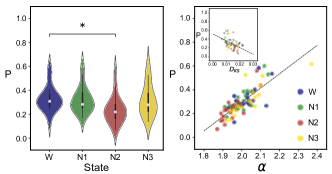
Figure 4: Model-based machine learning of critical brain dynamics. Left: Violin plots of the neural network output probabilities $P$ per sleep stage and participant (averaged across the $P$ obtained for all configurations corresponding to each sleep stage for each participant) (*p$<$0.05, Wilcoxon signed-rank test, Bonferroni corrected for all pairwise comparisons between wakefulness and sleep states). Right: Scatter plot of probabilities $P$ and power law exponents $\alpha$, one per subject and sleep stage. The dotted line indicates the best linear fit (least squares). A significant linear association between $P$ and $\alpha$ was found (R=0.81, p=1.3e-17). The inset shows a significant linear association between $P$ and $D_{ks}$ (R=-0.47, p=3.5e-5).

We conclude by showing that the changes in $\alpha$ (Fig. 3, lower left) could be explained by differences in the proximity to critical dynamics, according to the output of the neural network trained using the Greenberg-Hasting model. As shown in Fig. 4 (right), the $\alpha$ values estimated as the power law exponents of the cluster size distributions were highly correlated with $P$, the probability that the configuration corresponds to the supercritical phase (R=0.81, p=1.3e-17). We also show in figure inset a significant but lower negative correlation (R=-0.47, p=3.5e-5) between P probabilities and Kolmogorov-Smirnov distance ($D_{KS}$).

Discussion.— Recent studies have shown that supervised and unsupervised machine learning algorithms are capable of learning phase transitions in a variety of physical systems Wang (2016); Van Nieuwenburg et al. (2017); Carrasquilla and Melko (2017); Suchsland and Wessel (2018). Although phase transitions can be identified by a number of well understood signatures (typically associated with the appearance of scale-free distributions), none of these signatures are used directly as features to train the machine learning algorithms; instead, the information required to sort the phases of the system is inferred from the multivariate data. Here, we show that a neural network was not only capable of learning the phase transition in the Greenberg-Hastings model, but also reproduced changes in scaling parameters ($\alpha$) and goodness-of-fit statistics ($D_{KS}$) of power law fits when exposed to the full configuration vectors of the system. Consistently with previous reports Priesemann et al. (2014); Tomen et al. (2014), these changes are indicative of slightly subcritical dynamics, which are furthered in the progression from wakefulness to N2 sleep and restored during N3 sleep. This process could reflect the need to shift away from criticality until deep sleep is consolidated.

Synthetic data is considered valuable in machine learning problems where the number of training samples is scarce and data augmentation is required Perl et al. (2020); Van Dyk and Meng (2001). We showed that simulated data alone can be used to train a model capable of predicting the proximity to the critical point in real empirical data, as suggested by the correlation with the changes in $\alpha$. This suggests a general strategy to identify the phases of physical systems based on empirical data, whereby simulations provide the information to represent these phases in the parameters of a deep neural network, which is then used to furnish predictions based on empirical data. Importantly, the model we explored is not based on a realistic formulation of neural activity (although it incorporates realistic connectivity), suggesting that universal aspects of dynamics near a phase transition suffice to train the network. It is also important to note that our results do not constitute proof of changes in the proximity to critical dynamics; however, the output of the neural network can be taken as an additional signature to assess this possibility, which is not directly based on features such as $\alpha$ or $D_{KS}$ but learned from the integral dynamics of the model.

Specific applications of our development include the use of computational models to train algorithms capable of estimating levels of consciousness from brain imaging recordings, a problem of clinical relevance given the increasing number of patients who survive critical brain injury and enter a state of preserved vigilance, but with sporadic or inconsistent signs of conscious awareness Gosseries et al. (2014). For further validation we propose the application to physical systems theoretically known to undergo phase transitions that can be either controlled by the experimenter or inferred from multiple sources of high-quality empirical data.

Authors acknowledge funding from Agencia I+D+i, Argentina (grant PICT-2019-02294) and ANID/FONDECYT Regular 1220995 (Chile).

References

- Chialvo (2010) D. R. Chialvo, Nature physics 6, 744 (2010).
- Cocchi et al. (2017) L. Cocchi, L. L. Gollo, A. Zalesky, and M. Breakspear, Progress in neurobiology 158, 132 (2017).
- Kinouchi and Copelli (2006) O. Kinouchi and M. Copelli, Nature physics 2, 348 (2006).
- Shew and Plenz (2013) W. L. Shew and D. Plenz, The neuroscientist 19, 88 (2013).
- Beggs (2008) J. M. Beggs, Philosophical Transactions of the Royal Society A: Mathematical, Physical and Engineering Sciences 366, 329 (2008).
- Haimovici et al. (2013) A. Haimovici, E. Tagliazucchi, P. Balenzuela, and D. R. Chialvo, Physical review letters 110, 178101 (2013).
- Expert et al. (2011) P. Expert, R. Lambiotte, D. R. Chialvo, K. Christensen, H. J. Jensen, D. J. Sharp, and F. Turkheimer, Journal of The Royal Society Interface 8, 472 (2011).
- Hahn et al. (2017) G. Hahn, A. Ponce-Alvarez, C. Monier, G. Benvenuti, A. Kumar, F. Chavane, G. Deco, and Y. Frégnac, PLoS computational biology 13, e1005543 (2017).
- Tononi (2004) G. Tononi, BMC neuroscience 5, 1 (2004).
- Mashour et al. (2020) G. A. Mashour, P. Roelfsema, J.-P. Changeux, and S. Dehaene, Neuron 105, 776 (2020).
- Beggs and Timme (2012) J. M. Beggs and N. Timme, Frontiers in physiology 3, 163 (2012).
- Bak et al. (1988) P. Bak, C. Tang, and K. Wiesenfeld, Physical review A 38, 364 (1988).
- Beggs and Plenz (2003) J. M. Beggs and D. Plenz, Journal of neuroscience 23, 11167 (2003).
- Priesemann et al. (2014) V. Priesemann, M. Wibral, M. Valderrama, R. Pröpper, M. Le Van Quyen, T. Geisel, J. Triesch, D. Nikolić, and M. H. Munk, Frontiers in systems neuroscience 8, 108 (2014).
- Tagliazucchi et al. (2012) E. Tagliazucchi, P. Balenzuela, D. Fraiman, and D. R. Chialvo, Frontiers in physiology 3, 15 (2012).
- Shriki et al. (2013) O. Shriki, J. Alstott, F. Carver, T. Holroyd, R. N. Henson, M. L. Smith, R. Coppola, E. Bullmore, and D. Plenz, Journal of Neuroscience 33, 7079 (2013).
- Scott et al. (2014) G. Scott, E. D. Fagerholm, H. Mutoh, R. Leech, D. J. Sharp, W. L. Shew, and T. Knöpfel, Journal of Neuroscience 34, 16611 (2014).
- Girardi-Schappo (2021) M. Girardi-Schappo, Journal of Physics: Complexity (2021).
- Poil et al. (2008) S.-S. Poil, A. van Ooyen, and K. Linkenkaer-Hansen, Human brain mapping 29, 770 (2008).
- Tagliazucchi et al. (2016) E. Tagliazucchi, D. R. Chialvo, M. Siniatchkin, E. Amico, J.-F. Brichant, V. Bonhomme, Q. Noirhomme, H. Laufs, and S. Laureys, Journal of The Royal Society Interface 13, 20151027 (2016).
- Hagmann et al. (2008) P. Hagmann, L. Cammoun, X. Gigandet, R. Meuli, C. J. Honey, V. J. Wedeen, and O. Sporns, PLoS biology 6, e159 (2008).
- Fisch et al. (1993) R. Fisch, J. Gravner, and D. Griffeath, The Annals of Applied Probability 3, 935 (1993).
- Bocaccio et al. (2019) H. Bocaccio, C. Pallavicini, M. N. Castro, S. M. Sánchez, G. De Pino, H. Laufs, M. F. Villarreal, and E. Tagliazucchi, Journal of the Royal Society Interface 16, 20190262 (2019).
- Fisher (1967) M. E. Fisher, Physics Physique Fizika 3, 255 (1967).
- Clauset et al. (2009) A. Clauset, C. R. Shalizi, and M. E. Newman, SIAM review 51, 661 (2009).
- Wang (2016) L. Wang, Physical Review B 94, 195105 (2016).
- Van Nieuwenburg et al. (2017) E. P. Van Nieuwenburg, Y.-H. Liu, and S. D. Huber, Nature Physics 13, 435 (2017).
- Carrasquilla and Melko (2017) J. Carrasquilla and R. G. Melko, Nature Physics 13, 431 (2017).
- Suchsland and Wessel (2018) P. Suchsland and S. Wessel, Physical Review B 97, 174435 (2018).
- Tomen et al. (2014) N. Tomen, D. Rotermund, and U. Ernst, Frontiers in systems neuroscience 8, 151 (2014).
- Perl et al. (2020) Y. S. Perl, C. Pallavicini, I. P. Ipiña, M. Kringelbach, G. Deco, H. Laufs, and E. Tagliazucchi, Chaos, Solitons & Fractals 139, 110069 (2020).
- Van Dyk and Meng (2001) D. A. Van Dyk and X.-L. Meng, Journal of Computational and Graphical Statistics 10, 1 (2001).
- Gosseries et al. (2014) O. Gosseries, N. D. Zasler, and S. Laureys, Brain injury 28, 1141 (2014).