Rotating Lee-Wick Black Hole and Thermodynamics

Abstract

We derive a singular solution for the rotating counterpart of Lee-Wick gravity having a point source in a higher-derivative theory. We critically analyze the thermodynamics of such a thermal system by evaluating mass parameters, angular velocity, and Hawking temperature. The system follows the first law of thermodynamics and leads to the expression of entropy. We further discuss the stability and phase transition of the theory by evaluating heat capacity and free energy. The phase transition occurs at the point of divergence and the temperature is maximum. Remarkably, the black hole is unstable for a small horizon radius and stable for a large horizon radius.

I Introduction

Quantizing the theory of gravity is one of the most challenging tasks of theoretical physics. It is known that the gravity theory with forth derivative terms is renormalizable which in fact violate the unitarity of the theory [1]. However, the fourth derivative terms lead to the negative-norm states in the physical spectrum of the theory. This justifies instabilities in the classical solutions. A consistent theory of quantum gravity theory which agrees with both unitarity and renormalizability requires a modification in Einstein theory of gravity. One of the possible solutions to this problem is to consider a local gravitational theory with higher than fourth derivative terms. Such theories with higher derivatives terms have very interesting properties as they are superrenormalizable [2]. Also, these theories are unitary in the Lee-Wick formalism for the massive complex poles [3, 4]. Hence, these theories remove the conflict between unitarity and renormalizability in quantum gravity [5, 6, 7, 8, 9, 10, 11]. Also, the proof of unitarity of these models do not require any fine-tuning and therefore prove themselves as a better alternative to the non-local theories [12, 13, 14, 15, 16].

The singular solutions (black holes) are the most fundamental objects in gravity theory as they provide powerful probes to the study of various aspects of the theory. Therefore, the search of black-hole solutions in the higher-derivative gravity theories are of considerable interests. A static vacuum solution of an approximate equation of motion of the Lee-Wick gravity is studied recently where the solution is generated by a point-like massive source [17]. The authors of Ref. [17] discussed different scenarios by comparing the mass of the source with a critical value. They also shed light on the thermodynamics of these black holes and their evaporation process. The thermodynamics of the black hole plays a vital role in understanding the quantum theory of gravity [18, 19, 20, 21, 22]. Hawking and Page had found that the black hole solutions in asymptotically $AdS$ space have thermodynamic properties [23]. The rotational counterpart of these gravity theory remains unexplored. This provides us an opportunity to generalize the work and this is the motivation of present study.

In this paper, we obtain a rotating Lee-Wick black hole solution by using a modified Newman-Janis algorithm [24, 25, 26, 27]. To do so, we first convert static spherically symmetric Lee-Wick black hole solution into its rotational counterpart, we transform the coordinates of the Lee-Wick metric from the Boyer-Lindquist to the Eddington-Finkelstein. The numerical analysis leads to the possibilities to find non-vanishing values of rotation parameter which corresponds minimum metric function [28, 29]. We also investigate the basic thermodynamics properties of rotating Lee-Wick black hole. We first derive mass parameter and angular velocity. Moreover, we compute the Hawking temperature of rotating lee-Wick black hole in terms of temperature of Kerr black hole. A comparative analysis suggests that rotating Lee-Wick black holes with small rotation parameter are comparatively hotter. Also, the rotation parameter plays more significant role for small black holes. In order to study the stability of such black holes, we need to calculate heat capacity of the black hole and check the sign of heat capacity and free energy. Here, we find three phase transitions. For the stationary case when rotation parameter is switched-off, the phase transition occurs only once. In contrast, when rotation parameter acquires non-zero values, the phase transition occurs. Also, in stationary case, the larger black holes are stable.

The paper is organized as follows. In section II, we obtain a rotational counterpart of Lee-Wick black hole solution. In section III, we discussed the thermodynamics of rotational Lee-Wick black hole and studies their local and global stability. Finally, we conclude the work in the section V.

II Generating rotating Lee-Wick black hole solutions

. We start with the action of the minimal theory having unitarity with the Lee-Wick prescription [17]

$$S=\frac{1}{8\pi G_{N}}\int d^{4}x\sqrt{-g}\left[R+{\Lambda^{-4}}G_{\mu\nu}\Box R^{\mu\nu}\right],$$ (1)

where $R$ is the Ricci scalar, $\Lambda$ represents the UV scale of the theory and $G_{\mu\nu}$ is the Einstein tensor. Varying the action (1), we obtain the equations of motion (EoM)

$$\left(1+\frac{\Box^{2}}{\Lambda^{4}}\right)G_{\mu\nu}+O(R^{2}_{\mu\nu})=8\,\pi\,G_{N}T_{\mu\nu}$$ (2)

where energy momentum tensor (EMT) $T_{\mu\nu}=\left(1+{\Box^{2}}/{\Lambda^{4}}\right){\tilde{T}}_{\mu\nu}$. Ignoring higher-order ($O(R^{2}_{\mu\nu})$) terms, this EoM takes following form [17]:

$$G_{\mu\nu}=8\,\pi\,G\,\left(1+\frac{\Box^{2}}{\Lambda^{4}}\right)^{-1}{T}_{\mu\nu}.$$ (3)

The only non-vanishing component of EMT is $T_{t}^{t}=-M\delta(x)$ and, for this , the effective EMT is given by

$${\tilde{T}}^{\mu}_{\nu}=\text{diag}\left(-{\tilde{\rho}},{\tilde{P}_{r}},{\tilde{P}_{\theta}},{\tilde{P}_{\theta}}\right),$$ (4)

where ${\tilde{\rho}}$, ${\tilde{P}_{r}}$ and ${\tilde{P}_{\theta}}$ are the effective energy density, effective radial pressure and effective tengential pressure, repectively. The effective energy density is calculated as [17]

$$\tilde{\rho}=\left(1+\frac{\Box^{2}}{\Lambda^{4}}\right)^{-1} = -M\delta(x)=M\int\frac{dk^{3}}{(2\pi)^{3}}\frac{e^{ikx}}{1+k^{4}/\Lambda^{4}}$$ (5)

$$= \frac{M\Lambda^{2}}{4\pi r}\sin\frac{r\Lambda}{\sqrt{2}}e^{-\frac{r\Lambda}{\sqrt{2}}}.$$

Now, we write the static and spherically symmetric Lee-Wick solution which matches with the form of Schwarzschild metric as follows [17],

$$ds^{2}=-f(r)dt^{2}+\frac{dr^{2}}{f(r)}+r^{2}d\Omega_{2}^{2}\quad\text{with}\quad f(r)=1-\frac{2m(r)}{r}.$$ (6)

Here $m(r)$ refers to effective mass and depends on the radial coordinate ($r$) only due to the spherical symmetry. The expression for mass function $m(r)$ is given by [17]

$$m(r)=M\left[1-e^{-\frac{\Lambda r}{\sqrt{2}}}\left(1+\frac{\Lambda r}{\sqrt{2}}\right)\cos\left(\frac{\Lambda r}{\sqrt{2}}\right)+\frac{\Lambda r}{\sqrt{2}}\sin\left(\frac{\Lambda r}{\sqrt{2}}\right)\right],$$ (7)

where $\Lambda$ is the UV scale and $M$ corresponds to the mass of a static point-like source. It should be noted that this is not an exact solution of the equations of motion of the model (1) but rather a solution to the ‘approximate’ equations of motion (2) in [17] when the quadratic and higher-order terms in the Ricci tensor are neglected.

Upon effective mass expansion around the centre ($r=0$), one finds de Sitter core [17]

$$ds^{2}\approx-\left(1-\frac{\Lambda_{eff}r^{2}}{3}\right)dt^{2}+\frac{1}{\left(1-\frac{\Lambda_{eff}r^{2}}{3}\right)}dr^{2}+r^{2}d\Omega^{2}_{2}$$ (8)

where $\Lambda_{eff}=\sqrt{2}\Lambda^{3}M$ is the effective cosmological constant. The metric (8) describes a regular spacetime and thus curvature is singularity free.

Now, we proceed to obtain the rotating counterpart of the metric (6). In order to do so, we follow the method proposed originally by Newman and Janis [24] and further modified by Azreg-Ainou  [26]. In order to convert static spherically symmetric Lee-Wick black hole solution into its rotational counterpart, we first transform the coordinates of the spacetime metric (6) from the Boyer-Lindquist ($t,r,\theta,\phi$) to the Eddington-Finkelstein ($u,r,\theta,\phi$) as following:

$$du=dt-\frac{dr}{f(r)}.$$ (9)

This leads to the final spacetime metric in the following form:

$$ds^{2}=-fdu^{2}-2dudr+r^{2}d\theta^{2}+r^{2}\sin^{2}\theta d\phi^{2}.$$ (10)

It is known that contravariant components of the metric tensor in the advanced null Eddington-Finkelstein coordinates can be expressed by the null tetrad of the form

$$g^{\mu\nu}=-l^{\mu}n^{\nu}-l^{\nu}n^{\mu}+m^{\mu}\bar{m}^{\nu}+m^{\nu}\bar{m}^{\mu},$$ (11)

Following the method as discussed in Ref. [27], we first write the metric coordinates in null tetrad and do complex coordinate transformations in the $u-r$ plane as

$$u\rightarrow u-ia\cos\theta,\quad r\rightarrow r-ia\cos\theta.$$ (12)

This converts the metric functions into a new form: $f(r)\rightarrow F(r,a,\theta)$, $r^{2}\rightarrow\Sigma(r,a,\theta)$. Furthermore, null tetrads also take the following new form:

$$l^{\mu}=\delta_{r}^{\mu}\ ,\quad m^{\mu}=\frac{1}{\sqrt{2\Sigma}}\left[\delta_{\theta}^{\mu}+ia\sin\theta(\delta_{u}^{\mu}-\delta_{r}^{\mu})+\frac{i}{\sin\theta}\delta_{\phi}^{\mu}\right]\ ,$$

$$n^{\mu}=\sqrt{\frac{G}{F}}\delta_{u}^{\mu}-\frac{1}{2}F\delta_{r}^{\mu}\ ,\quad\bar{m}^{\mu}=\frac{1}{\sqrt{2\Sigma}}\left[\delta_{\theta}^{\mu}-ia\sin\theta(\delta_{u}^{\mu}-\delta_{r}^{\mu})-\frac{i}{\sin\theta}\delta_{\phi}^{\mu}\right].$$ (13)

Then we can rewrite the contravariant components of the metric tensor $g^{\mu\nu}$ by using (11) as

$$g^{\mu\nu}=\left(\begin{array}[]{c c c c}a^{2}\sin^{2}\theta/\Sigma&-\sqrt{G/F}-a^{2}\sin^{2}\theta/\Sigma&0&a/\Sigma\\ -\sqrt{G/F}-a^{2}\sin^{2}\theta/\Sigma&G+a^{2}\sin^{2}\theta/\Sigma&0&-a/\Sigma\\ 0&0&1/\Sigma&0\\ a/\Sigma&-a/\Sigma&0&1/(\Sigma\sin^{2}\theta)\\ \end{array}\right).$$ (18)

The covariant components read

$$g_{\mu\nu}=\left(\begin{array}[]{c c c c}-F&-\sqrt{\frac{F}{G}}&0&a\left(F-\sqrt{\frac{F}{G}}\right)\sin^{2}\theta\\ -\sqrt{\frac{F}{G}}&0&0&a\sqrt{\frac{F}{G}}\sin^{2}\theta\\ 0&0&\Sigma&0\\ a\left(F-\sqrt{\frac{F}{G}}\right)\sin^{2}\theta&a\sqrt{\frac{F}{G}}\sin^{2}\theta&0&\sin^{2}\theta\left[\Sigma+a^{2}\left(2\sqrt{\frac{F}{G}}-F\right)\sin^{2}\theta\right]\\ \end{array}\right).$$ (23)

The last step of the algorithm is to turn back from the Eddington-Finkelstein coordinates to the Boyer-Lindquist coordinates by using the following coordinate transformations:

$$du=dt+\lambda(r)dr\ \qquad\text{and}\qquad\quad d\phi=d\phi+\chi(r)dr\ .$$ (24)

The transformation functions $\lambda(r)$ and $\chi(r)$ are found due to the requirement that, except the coefficient $g_{t\phi}$ ($g_{\phi t}$), all the non-diagonal components of the metric tensor are equal to zero. Thus

$$\lambda(r)=-\frac{r^{2}+a^{2}}{f(r)^{2}+a^{2}}\ ,\qquad\qquad\qquad\qquad\chi(r)=-\frac{a}{f(r)r^{2}+a^{2}},$$

$$F(r,\theta)=\frac{(f^{2}+a^{2}\cos^{2}\theta)\Sigma}{(r^{2}+a^{2}\cos^{2}\theta)^{2}},\qquad\text{and}\qquad G(r,\theta)=\frac{f^{2}+a^{2}\cos^{2}\theta}{\Sigma}.$$ (25)

Consequently, we obtain the following line-element for the rotational counterpart of the Lee-Wick black hole solution

$$ds^{2} = -\left(1-\frac{2Mr-2Me^{-\frac{\Lambda r}{\sqrt{2}}}\left[\left(1+\frac{\Lambda r}{\sqrt{2}}\right)\cos\frac{\Lambda r}{\sqrt{2}}+\sin\frac{\Lambda r}{\sqrt{2}}\right]}{r^{2}+a^{2}\cos^{2}\theta}\right)dt^{2}+\frac{r^{2}+a^{2}\cos^{2}\theta}{\Delta}dr^{2}$$ (26)

$$- 2a\sin^{2}\theta\left(\frac{2Mr-2Me^{-\frac{\Lambda r}{\sqrt{2}}}\left[\left(1+\frac{\Lambda r}{\sqrt{2}}\right)\cos\frac{\Lambda r}{\sqrt{2}}+\sin\frac{\Lambda r}{\sqrt{2}}\right]}{r^{2}+a^{2}\cos^{2}\theta}\right)d\phi dt+(r^{2}+a^{2}\cos^{2}\theta)d\theta^{2}$$

$$+ \sin^{2}\theta\left[r^{2}+a^{2}+a^{2}\sin^{2}\theta\left(\frac{2Mr-2Me^{-\frac{\Lambda r}{\sqrt{2}}}\left[\left(1+\frac{\Lambda r}{\sqrt{2}}\right)\cos\frac{\Lambda r}{\sqrt{2}}+\sin\frac{\Lambda r}{\sqrt{2}}\right]}{r^{2}+a^{2}\cos^{2}\theta}\right)\right]d\phi^{2},$$

with

$$\Delta=r^{2}-2Mr+a^{2}+2Me^{-\frac{\Lambda r}{\sqrt{2}}}\left[\left(1+\frac{\Lambda r}{\sqrt{2}}\right)\cos\frac{\Lambda r}{\sqrt{2}}+\sin\frac{\Lambda r}{\sqrt{2}}\right],$$ (27)

where $a$ is the rotation parameter of black hole. Arising from the UV scale theory, $\Lambda$ measures the potential deviation from the Kerr metric. The obtained black hole solution (26) is independent of $t,\phi$, which implies that it admits two Killing vectors given by $\eta^{\mu}=\delta^{\mu}_{t}$ and $\xi^{\mu}=\delta^{\mu}_{\phi}$. The horizons of rotating Lee-Wick black holes are solution of equation $(\eta^{\mu}\xi_{\mu})^{2}-(\eta_{\mu}\eta^{\mu})(\xi_{\nu}\xi^{\nu})=0$, which gives

$$g_{t\phi}^{2}-g_{tt}g_{\phi\phi}=0.$$ (28)

Here, this yields

$$r^{2}-2Mr+a^{2}+2Me^{-\frac{\Lambda r}{\sqrt{2}}}\left[\left(1+\frac{\Lambda r}{\sqrt{2}}\right)\cos\frac{\Lambda r}{\sqrt{2}}+\sin\frac{\Lambda r}{\sqrt{2}}\right]=0.$$ (29)

This is a transcendental equation which cannot be solved analytically. The numerical analysis of the $\Delta=0$ on varying the angular momentum $a$ with fixed mass $M=1$ is depicted in the Fig. 1. The numerical analysis of $\Delta=0$ reveals that it is possible to find non-vanishing value of angular momentum ($a$) and UV scale parameter $x=\Lambda r/\sqrt{2}$ for which metric function $\Delta$ is minimum, i.e, $\Delta(x_{+})=0$ and this will give two real roots $x_{+}$ and $x_{-}$which correspond to the Cauchy horizon and event horizon.

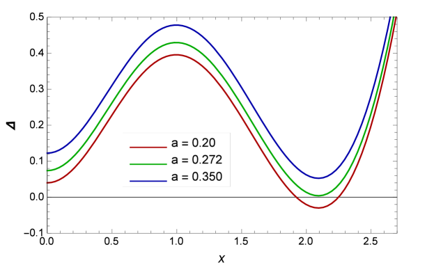
Figure 1: The plot of metric function $\Delta(r)$ as the function of dimensionless parameter $x=\Lambda r/\sqrt{2}$ for different values of angular momentum $a$ with fixed value of $\Lambda=4\sqrt{2}\pi$.

$a$	$x_{+}$	$x_{-}$	$\delta=x_{+}-x_{-}$
0.10	1.85	2.31.	0.46
0.20	1.92	2.24	0.32
0.272	2.096	2.096	0

Table 1: The table for horizon radius for different value of rotation parameter $a$ with fixed value of $\Lambda=4\sqrt{2}\pi$.

From the Fig. (1) and Table 1, we can see that the horizon of the black hole decreases with increasing rotation parameter and at $a=0.268$ two horizons reduces to one, i.e., $r_{\pm}=r_{E}$ such that $\Delta(r_{E})=\Delta^{\prime}{r_{E}}=0$.

III Thermodynamics

In this section, we analyse the thermodynamics of the rotating Lee-Wick black hole described by metric  (26). Let us begin by deriving the mass by $g^{rr}=0$ as following:

$$M_{+}=\frac{\left(a^{2}+r_{+}^{2}\right)}{2r_{+}\left(1-e^{-\frac{\Lambda r_{+}}{\sqrt{2}}}\left(\left(1+\frac{\Lambda r_{+}}{\sqrt{2}}\right)\cos\left[\frac{\Lambda r_{+}}{\sqrt{2}}\right]+\frac{\Lambda r_{+}}{\sqrt{2}}\sin\left[\frac{\Lambda r_{+}}{\sqrt{2}}\right]\right)\right)}.$$ (30)

In the absence of rotation parameter ($a$), the mass (30) reduces to the mass of Lee-Wick black hole [17]; however this reduces to mass of Kerr black hole in the limit of $\Lambda\to 0$.

For the stationary axially symmetric metric like (26), we have two associated Killing vectors $\eta^{\mu}=\partial_{t}$ corresponding to the time translational symmetry along the $t$-axis and $\xi^{\mu}=\partial_{\phi}$ corresponding to the rotational symmetry about $\phi$-axis. In therms of these killing vectors a Killing field $\chi{{}^{\mu}}$ can be expressed as $\chi{{}^{\mu}}=\eta^{\mu}+\Omega\xi^{\mu}$, where $\Omega$ refers to the angular velocity of the metric. Being a null vector at the event horizon (i.e. $\chi{{}^{\mu}}\chi_{\mu}=0$), the Killing field decides the angular velocity and leads to [30, 31]

$$g_{tt}+2\Omega g_{t\phi}+\Omega^{2}g_{\phi\phi}=0,$$ (31)

where angular velocity is given by

$$\Omega = -\frac{g_{t\phi}}{g_{\phi\phi}}\pm\sqrt{\left(\frac{g_{t\phi}}{g_{\phi\phi}}\right)^{2}-\frac{g_{tt}}{g_{\phi\phi}}},$$ (32)

$$= \frac{-a\left[\Sigma-(\Delta-a^{2}\sin^{2}\theta)\right]}{\Sigma^{2}+a^{2}\sin^{2}\theta\left[2\Sigma-(\Delta-a^{2}\sin^{2}\theta)^{2}\right]}$$

$$\pm \frac{\Sigma\Delta^{\frac{1}{2}}}{\sin\theta\left[(a^{2}\sin^{2}\theta+\Sigma)^{2}-\Delta a^{2}\sin^{2}\theta\right]}.$$

In terms of horizon radius, the angular velocity reads

$$\Omega_{+}=-\left.\frac{g_{t\phi}}{g_{\phi\phi}}\right|_{r=r_{+}}=\frac{a}{r_{+}^{2}+a^{2}}.$$ (33)

Before computing temperature of the black holes, it is worth to first work out the surface gravity at the event horizon for the obtained solution (26). This gives

$$\kappa=\sqrt{-\frac{\nabla_{\mu}\chi{{}_{\nu}}\nabla{{}^{\mu}}\chi{{}^{\nu}}}{2}}=\frac{\Delta^{\prime}(r_{+})}{2(r_{+}^{2}+a^{2})}.$$ (34)

Here ^′ denotes differentiation with respect to horizon radius. Utilizing the standard relation of Surface gravity and Hawking temperature $T_{+}=\kappa/2\pi$, we obtain the Hawking temperature of the rotating Lee-Wick black hole metric (26) as

$$T_{+}=T_{+}^{Kerr}\left[\frac{e^{-\frac{r_{+}\Lambda}{\sqrt{2}}}\left(\left(1+\frac{\Lambda r_{+}}{\sqrt{2}}\right)\cos\left[\frac{\Lambda r_{+}}{\sqrt{2}}\right]+r_{+}\left(\frac{\Lambda r_{+}}{\sqrt{2}}+\frac{\Lambda}{2}\left(\frac{a^{2}+r_{+}^{2}}{a^{2}-r_{+}^{2}}\right)\right)\sin\left[\frac{\Lambda r_{+}}{\sqrt{2}}\right]\right)-1}{e^{-\frac{r_{+}\Lambda}{\sqrt{2}}}\left(\left(1+\frac{\Lambda r_{+}}{\sqrt{2}}\right)\cos\left[\frac{\Lambda r_{+}}{\sqrt{2}}\right]+\frac{\Lambda r_{+}}{\sqrt{2}}\sin\left[\frac{\Lambda r_{+}}{\sqrt{2}}\right]-r_{+}\right)}\right],$$ (35)

where $T_{+}^{Kerr}={\left(r_{+}^{2}-a^{2}\right)}/{\left(4\pi r_{+}(r_{+}^{2}+a^{2})\right)}$ is the temperature of the Kerr black hole. The temperature (35) reduces to the temperature of the Kerr black hole in the limit of $\Lambda\to 0$.

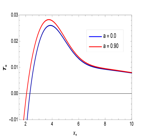
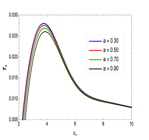
Figure 2: The plot of Hawking temperature $T_{+}$ versus horizon radius $x_{+}$ for different values of rotation parameter $a$ with fixed Value of $\Lambda=4\sqrt{2}\pi$.

$a$	$0.30$	$0.50$	$0.70$	$0.90$
$T_{max}$	0.0279	0.0275.	0.0268	0.0260
$x_{c}$	3.750	3.797	3.816	3.872

Table 2: The table for temperature for different value of rotation paramete $a$ with fixed value of $\Lambda=4\sqrt{2}\pi$.

From the Fig. 2 and table (2), it is clear that the black hole becomes hotter for small rotation parameter and the critical radius increases with the rotation parameter $(a)$. The maximum Hawking temperature decreases for higher values of the critical radius $(r_{c})$. Thus, This signifies that the effect of rotation parameter is more significant for small black holes.

This black hole can be considered as a thermodynamic system only if the quantities associated with it must satisfies the first-law of thermodynamics

$$dM_{+}=T_{+}dS_{+}+\Omega_{+}da.$$ (36)

The validity of above relation leads to the expression for entropy

$$S=-4\pi\int dr_{+}\frac{(a^{2}+r_{+}^{2})e^{-r_{+}\Lambda/\sqrt{2}}}{e^{-\frac{\Lambda r_{+}}{\sqrt{2}}}\left(\left(2+{\sqrt{2}}\,r_{+}\Lambda\right)\cos\left[\frac{\Lambda r_{+}}{\sqrt{2}}\right]+{\sqrt{2}}\sin\left[\frac{\Lambda r_{+}}{\sqrt{2}}\right]\right)}.$$ (37)

From this this expression it is clear that the entropy does not depends upon roation parameter ($a$). The entropy is the function of horizon radius which is depicted in Fig. (3)

$\begin{array}[]{c c c c}\includegraphics[width=325.215pt]{s.eps}\end{array}$

Figure 3: The plot of entropy $S_{+}$ vs $x_{+}$ with fixed value of $\Lambda=4\sqrt{2}\pi$.

The definition of first-law of thermodynamics is worth mentioning to check the validity of these thermodynamic quantities. It is easy to verify the complete form of the first-law of thermodynamics as

$$dM_{+}=T_{+}dS_{+}+\Omega_{+}dJ$$ (38)

Substituting the value of mass, temperature and entropy from the Eqs. (30), (35) and (37), respectively, given in Eq. (38), we can see that the rotating Lee-Wick black hole follows the first-law of thermodynamics.

IV Local and Global Stability

Finally, we study the thermodynamic stability of rotating Lee-Wick black hole by estimating the heat capacity. The stability of the black hole can be estimated from sign of the heat capacity ($C_{+}$) as positive heat capacity reflects the stable black hole and negative reflects the unstable one. The heat capacity of the black hole can be calculated by [30, 31, 32, 33]

$$C_{+}=\frac{dM_{+}}{dT_{+}}=\frac{dM_{+}}{dr_{+}}\frac{dr_{+}}{dT_{+}}$$ (39)

substituting the mass and temperature from Eq. (30) and Eq. (35) into Eq. (39) we get

$$C_{+}=2\pi\frac{\left(r^{2}-a^{2}\right)\left(r^{2}+a^{2}\right)^{2}Y}{X},$$ (40)

with

$$Y = e^{-\frac{\Lambda r_{+}}{\sqrt{2}}}\left(\left(1+\frac{\Lambda r_{+}}{\sqrt{2}}\right)\cos\left[\frac{\Lambda r_{+}}{\sqrt{2}}\right]+r_{+}\left(\frac{\Lambda r_{+}}{\sqrt{2}}+\frac{\Lambda}{2}\left(\frac{a^{2}+r_{+}^{2}}{a^{2}-r_{+}^{2}}\right)\right)\sin\left[\frac{\Lambda r_{+}}{\sqrt{2}}\right]\right)-1,$$

$$X = 2\left(a^{4}+4a^{2}r_{+}^{2}-r_{+}^{4}\right)\left[\left(e^{\frac{{\Lambda r_{+}}}{\sqrt{2}}}-\cos\left[\frac{\Lambda r_{+}}{\sqrt{2}}\right]\right)^{2}+\frac{{2\Lambda r_{+}}}{\sqrt{2}}\left(e^{\frac{{\Lambda r_{+}}}{\sqrt{2}}}-\cos\left[\frac{\Lambda r_{+}}{\sqrt{2}}\right]\right)\right.$$ (41)

$$\left.\left(\sin\left[\frac{\Lambda r_{+}}{\sqrt{2}}\right]+\cos\left[\frac{\Lambda r_{+}}{\sqrt{2}}\right]\right)-2\left(\frac{\Lambda r_{+}}{\sqrt{2}}\right)^{2}\right]+4\left(r_{+}^{2}+a^{2}\right)^{2}\left[-\left(\frac{\Lambda r_{+}}{\sqrt{2}}\right)^{2}\right.$$

$$+ \left.\left(\frac{\Lambda r_{+}}{\sqrt{2}}\right)^{7}\left(e^{-\frac{{\Lambda r_{+}}}{\sqrt{2}}}-\left(\cos\left[\frac{\Lambda r_{+}}{\sqrt{2}}\right]-\sin\left[\frac{\Lambda r_{+}}{\sqrt{2}}\right]\right)\right)\right].$$

$\begin{array}[]{c c c c}\includegraphics[width=325.215pt]{4.eps}\end{array}$

Figure 4: The plot of specific heat $C_{+}$ as the function of dimensionless parameter $x=\Lambda r/\sqrt{2}$ for different values of angular momentum $a$ with fixed value of $\Lambda=4\sqrt{2}\pi$.

In order to study the stability of rotating Lee-Wick black hole, we plot the heat capacity with respect to dimensionless parameter $x$ in Fig 5. From Eq. (40), it can be observed that the specific heat diverges at $r_{+}=3.75$ this discontinuity of the heat capacity represents a point of phase transition.

$\begin{array}[]{c c c c}\includegraphics[width=325.215pt]{free.eps}\end{array}$

Figure 5: The plot of free energy $C_{+}$ as the function of dimensionless parameter $x=\Lambda r/\sqrt{2}$ for different values of angular momentum $a$ with fixed value of $\Lambda=4\sqrt{2}\pi$.

Now, we study the behaviour of Gibbs free energy for the global stability of black hole thermodynamics. The definition of Gibbs free energy is given by

$$G_{+}=M_{+}-T_{+}S_{+}.$$ (42)

Substituting the mass, temperature and entropy from Eqs. (30), (35) and (37) into (42) we get

$$G_{+} = \frac{\left(a^{2}+r_{+}^{2}\right)}{2r_{+}\left(1-e^{-\frac{\Lambda r_{+}}{\sqrt{2}}}\left(\left(1+\frac{\Lambda r_{+}}{\sqrt{2}}\right)\cos\left[\frac{\Lambda r_{+}}{\sqrt{2}}\right]+\frac{\Lambda r_{+}}{\sqrt{2}}\sin\left[\frac{\Lambda r_{+}}{\sqrt{2}}\right]\right)\right)}+\left(\frac{r_{+}^{2}-a^{2}}{4\pi(r_{+}^{2}+a^{2})}\right)$$ (43)

$$\left(\frac{e^{-\frac{r_{+}\Lambda}{\sqrt{2}}}\left(\left(1+\frac{\Lambda r_{+}}{\sqrt{2}}\right)\cos\left[\frac{\Lambda r_{+}}{\sqrt{2}}\right]+r_{+}\left(\frac{\Lambda r_{+}}{\sqrt{2}}+\frac{\Lambda}{2}\left(\frac{a^{2}+r_{+}^{2}}{a^{2}-r_{+}^{2}}\right)\right)\sin\left[\frac{\Lambda r_{+}}{\sqrt{2}}\right]\right)-1}{e^{-\frac{r_{+}\Lambda}{\sqrt{2}}}\left(\left(1+\frac{\Lambda r_{+}}{\sqrt{2}}\right)\cos\left[\frac{\Lambda r_{+}}{\sqrt{2}}\right]+\frac{\Lambda r_{+}}{\sqrt{2}}\sin\left[\frac{\Lambda r_{+}}{\sqrt{2}}\right]-r_{+}\right)}\right)$$

$$\int dr_{+}\frac{(a^{2}+r_{+}^{2})e^{-r_{+}\Lambda/\sqrt{2}}}{e^{-\frac{\Lambda r_{+}}{\sqrt{2}}}\left(\left(2+{\sqrt{2}}\,r_{+}\Lambda\right)\cos\left[\frac{\Lambda r_{+}}{\sqrt{2}}\right]+{\sqrt{2}}\sin\left[\frac{\Lambda r_{+}}{\sqrt{2}}\right]\right)}.$$

We analyse the stability of the black hole by studying the nature of free energy which is plotted for the different values of rotation parameter $(a)$ in Fig. 5. Here we see that the free energy has a maximum value where the specific heat diverges (see Fig. 4) which can be identified as the extremal points of the Hawking temperature (see Fig. 2). We also notice that the rotating black hole is unstable for small values of $r_{+}$ and stable for large horizon radius. It means that the large black hole is stable.

V Conclusions

We have extended the investigation of static and spherically symmetric Lee- Wick solution. In fact, we have obtained a rotating Lee-Wick black hole solution by exploiting a corrected Newman-Janis algorithm. Specifically, in order to derive a rotational counterpart, we first considered static spherically symmetric Lee-Wick black hole solution and made a coordinate transformation from the Boyer-Lindquist coordinates to the Eddington-Finkelstei coordinates. Moreover, we have written the contravariant components of the metric tensor in the advanced null Eddington-Finkelstei coordinates in the null tetrad form. After that we have performed a complex coordinate transformations followed by the coordinate transformation in order to retain the metric in Boyer-Lindquist coordinates. Since we are left with a transcendental equation which can not be solved analytically. Hence, we have tried to do a numerical analysis by comparing the metric function $\Delta$ equal to zero which reveals the possibilities for finding the non-zero values of angular momentum and cosmological constant.

Also, we have discussed the basic thermodynamics properties of this rotating Lee-Wick black hole. In order to do so, first we have evaluated a mass parameter and angular velocity. Following standard black hole chemistry from areal-law, we have derived the Hawking temperature of rotating Lee-Wick black hole and expressed in terms of temperature of Kerr black hole. In order to study the behaviour of black hole with horizon radius, we have plotted a graph and found that the temperature of rotating Lee-Wick black holes is increasing for smaller rotation parameter. We also found that the effects of rotation parameter become more significant for relatively smaller black holes. The stability of this black holes is studied by evaluating heat capacity of the black hole and checking the sign of heat capacity. Remarkably, the system exhibits various phase transitions. A comparative analysis is done and found that for the stationary case (when rotation parameter is turned-off) the phase transition occurs only once for small sized black holes. In contrast, when rotation parameter acquires non-zero values, the phase transition occurred at various points. The graph signified that in contrast to the stationary case, we have found a stable region for the larger rotating black holes also. The results of the paper are quite interesting and yields new insight for future investigations.

Appendix A Verification of black hole solution by equation of motion

In order to compute the energy momentum tensor, we use the following tetrad

$$e^{\mu}_{t}=\frac{1}{\Sigma\sqrt{\Delta}}(r^{2}+a^{2},0,0,a),$$ (44)

$$e^{\mu}_{r}=\frac{\sqrt{\Delta}}{\Sigma}(0,1,0,0),$$ (45)

$$e^{\mu}_{\theta}=\frac{1}{\Sigma}(0,0,1,0),$$ (46)

$$e^{\mu}_{\phi}=-\frac{1}{\Sigma\sin\theta}(r^{2}+a^{2},0,0,a).$$ (47)

The non-zero component of energy momentum tensor are given by

$${\tilde{\rho}(r)}=-{\tilde{P}}_{r}=\frac{M\Lambda^{2}}{4\pi r}\sin\frac{r\Lambda}{\sqrt{2}}e^{-\frac{r\Lambda}{\sqrt{2}}},$$ (48)

$${\tilde{P}}_{\theta}={\tilde{P}}_{\phi}=\frac{M\Lambda^{2}e^{-\frac{r\Lambda}{\sqrt{2}}}}{16\pi r}\left(\sqrt{2}\cos\frac{r\Lambda}{\sqrt{2}}+(2-\sqrt{2}r)\sin\frac{r\Lambda}{\sqrt{2}}-8\sin\frac{r\Lambda}{\sqrt{2}}\frac{M-rM^{\prime}}{2M-r}\right).$$ (49)

The equation of motion of the action (1) can be written as

$$G_{t}^{t} = -\frac{1}{4\Sigma^{2}(f(r,\theta)E(r,\theta)+B(r,\theta))^{2}}\Big{[}-E^{2}\,f\,\frac{\Sigma}{\Delta}\Delta^{\prime}-E^{2}f\left(\frac{\Sigma}{\Delta}\right)^{\prime 2}\Delta$$ (50)

$$- EB^{2}\Delta^{\prime 2}\frac{\Sigma}{\Delta}-E\Delta B^{2}\left(\frac{\Sigma}{\Delta}\right)^{\prime 2}+2\Sigma\Delta E^{\prime\prime}fE+2E\left(\frac{\Sigma}{\Delta}\right)^{\prime\prime}\Sigma B^{2}+2E\Delta^{\prime\prime}\Sigma B^{2}$$

$$+ 2E^{2}f\left(\frac{\Sigma}{\Delta}\right)^{\prime\prime}\Sigma+2\left(\frac{\Sigma}{\Delta}\right)^{2}\Delta E^{\prime\prime}B^{2}+2E^{2}f\Delta^{\prime\prime}\Sigma-E^{2}f\Delta^{\prime}\left(\frac{\Sigma}{\Delta}\right)^{\prime}\frac{\Sigma}{\Delta}$$

$$- E^{2}f\left(\frac{\Sigma}{\Delta}\right)^{\prime}\Delta^{\prime}\Delta-E\left(\frac{\Sigma}{\Delta}\right)^{\prime}\Delta^{\prime}\Delta B^{2}-E\left(\frac{\Sigma}{\Delta}\right)^{\prime}\Delta^{\prime}\frac{\Sigma}{\Delta}B^{2}+\left(\frac{\Sigma}{\Delta}\right)\Delta B^{\prime}E$$

$$+ \left(\frac{\Sigma}{\Delta}\right)^{2}\Delta B^{\prime}E-\left(\frac{\Sigma}{\Delta}\right)^{\prime}\Delta^{\prime}E^{\prime}B^{2}+2\Sigma\Delta E^{\prime\prime}fE+\left(\frac{\Sigma}{\Delta}\right)^{\prime}\Sigma E^{\prime}fE$$

$$+ \Delta^{\prime}\Sigma E^{\prime}fE-2\Sigma\Delta BB^{\prime}E^{\prime}-2\left(\frac{\Sigma}{\Delta}\right)^{2}\Delta BB^{\prime}E^{\prime}-\left(\frac{\Sigma}{\Delta}\right)^{\prime}\Delta^{2}E^{\prime}fE$$

$$- \left(\frac{\Sigma}{\Delta}\right)^{\prime}\left(\frac{\Sigma}{\Delta}\right)\Delta E^{\prime}B^{2}-\Delta^{\prime}\left(\frac{\Sigma}{\Delta}\right)^{2}E^{\prime}fE-\Delta^{\prime}\Sigma E^{\prime}B^{2}-E^{\prime 2}\Sigma\Delta f$$

$$- \Delta^{\prime}\left(\frac{\Sigma}{\Delta}\right)^{2}E^{\prime}B^{2}-E^{\prime 2}\left(\frac{\Sigma}{\Delta}\right)^{2}\Delta f\Big{]},$$

$$G^{t}_{\phi} = -\frac{1}{4\Sigma^{2}(f(r,\theta)E(r,\theta)+B(r,\theta))^{2}}\Big{[}\Delta^{\prime 2}\frac{\Sigma}{\Delta}B^{3}+\left(\frac{d}{d\theta}\frac{\Sigma}{\Delta}\right)^{2}\Delta B^{3}$$ (51)

$$+ EfB\left(\frac{d}{d\theta}\frac{\Sigma}{\Delta}\right)^{2}\Delta+EfB\Delta^{\prime 2}\frac{\Sigma}{\Delta}-2EfB\left(\frac{d^{2}}{d\theta^{2}}\frac{\Sigma}{\Delta}\right)\Sigma-2B^{\prime\prime}\Sigma\Delta fE$$

$$- 2B^{\prime\prime}\frac{\Sigma^{2}}{\Delta}fE-\frac{dB}{d\theta}\frac{dC}{d\theta}\Sigma fE-2EfB\Delta^{\prime\prime}\Sigma-B^{\prime}\Delta^{\prime}\Sigma fE-2EfB\Delta^{\prime\prime}\Sigma$$

$$- f^{\prime}\Sigma\Delta BE^{\prime}+\frac{dA}{d\theta}\frac{dB}{d\theta}\frac{\Sigma^{2}}{\Delta}E-\frac{dA}{d\theta}\frac{dE}{d\theta}\frac{\Sigma^{2}}{\Delta}B+B^{\prime}C^{\prime}\Delta^{2}fE$$

$$- \frac{dB}{d\theta}\frac{dC}{d\theta}\Sigma B^{2}+E^{\prime}\Sigma\Delta fB^{\prime}+\frac{dB}{d\theta}\frac{d\Delta}{d\theta}\frac{\Sigma^{2}}{\Delta^{2}}fE-B^{\prime}\Delta^{\prime}\Sigma B^{2}+\frac{dE}{d\theta}\frac{dB}{f}\frac{\Sigma^{2}}{\Delta}{d\theta}$$

$$- 2B^{\prime\prime}\Sigma\Delta B^{2}-2\frac{d^{2}B}{d\theta^{2}}B^{2}\frac{\Sigma^{2}}{\Delta}+EfBC^{\prime}\Delta^{\prime}\Delta+EfB\frac{dC}{d\theta}\frac{d\Delta}{d\theta}\frac{\Sigma}{\Delta}-2\Delta^{\prime\prime}\Sigma B^{3}$$

$$+ C^{\prime}\Delta^{\prime}\Delta B^{3}+B\Sigma\Delta B^{\prime\prime}+B\frac{\Sigma^{2}}{\Delta}\left(\frac{dB}{d\theta}\right)^{2}+B^{\prime}C^{\prime}\Delta^{2}B^{2}+\frac{dB}{d\theta}\frac{d\Delta}{d\theta}\frac{\Sigma^{2}}{\Delta^{2}}$$

$$+ A^{\prime}\Sigma\Delta EB^{\prime}-2\frac{d^{C}}{d\theta^{2}}\Delta B^{3}\Big{]},$$

$$G^{r}_{r} = \frac{1}{4\Sigma^{2}(f(r,\theta)E(r,\theta)+B(r,\theta))^{2}}\Big{[}\Delta^{2}B^{\prime 2}B^{2}+2\Delta^{\prime}\Delta B^{3}B^{\prime}-\Sigma B^{2}\left(\frac{dB}{d\theta}\right)^{2}$$ (52)

$$- \Sigma E^{2}\left(\frac{dA}{d\theta}\right)^{2}-2\left(\frac{d\Delta}{d\theta}\right)\frac{\Sigma}{\Delta}B^{3}\left(\frac{dB}{d\theta}\right)-\Sigma f^{2}\left(\frac{dE}{d\theta}\right)^{2}+\Delta^{2}B^{\prime 2}fE$$

$$+ \Delta^{2}E^{\prime}f^{\prime}B^{2}+2\Delta^{\prime}\Delta BB^{\prime}fE+\Sigma\left(\frac{dE}{d\theta}\right)\left(\frac{df}{d\theta}\right)fE-4\Sigma EB\left(\frac{df}{d\theta}\right)\left(\frac{dB}{d\theta}\right)$$

$$- 4\Sigma Bf\left(\frac{dB}{d\theta}\right)\left(\frac{dE}{d\theta}\right)-2\left(\frac{d\Delta}{d\theta}\right)\left(\frac{dB}{d\theta}\right)\frac{\Sigma}{\Delta}BfE+3\Sigma\left(\frac{dE}{d\theta}\right)\left(\frac{df}{d\theta}\right)B^{2}$$

$$+ 3\Sigma\left(\frac{dE}{d\theta}\right)\left(\frac{dA}{d\theta}\right)B^{2}+3\Sigma\left(\frac{dB}{d\theta}\right)^{2}fE-\left(\frac{d\Delta}{d\theta}\right)\frac{\Sigma}{\Delta}E^{2}f\left(\frac{df}{d\theta}\right)$$

$$- \left(\frac{d\Delta}{d\theta}\right)\frac{\Sigma}{\Delta}EB^{2}\left(\frac{dA}{d\theta}\right)-\left(\frac{d\Delta}{d\theta}\right)\frac{\Sigma}{\Delta}A^{2}E\left(\frac{dE}{d\theta}\right)-\left(\frac{d\Delta}{d\theta}\right)\frac{\Sigma}{\Delta}fB^{2}\left(\frac{dE}{d\theta}\right)$$

$$+ \Delta^{2}E^{\prime}f^{\prime}fE+\Delta^{\prime}\Delta E^{2}f^{\prime}f+\Delta^{\prime}\Delta Ef^{\prime}B^{2}+\Delta^{\prime}\Delta fE^{\prime}E+\Delta^{\prime}\Delta fE^{\prime}B^{2}$$

$$+ 4\Sigma B\left(\frac{dB}{d\theta^{2}}\right)fE+4\Sigma E^{2}\left(\frac{d^{2}f}{d\theta^{2}}\right)f+2\Sigma fB^{2}\left(\frac{d^{E}}{d\theta^{2}}\right)+2\Sigma f^{2}\left(\frac{d^{2}E}{d\theta^{2}}\right)E$$

$$+ 2\Sigma E\left(\frac{d^{2}A}{d\theta^{2}}\right)B^{2}+4\Sigma B^{2}\left(\frac{d^{2}B}{d\theta^{2}}\right)\Big{]},$$

$$G_{\theta}^{\theta} = \frac{1}{4\Sigma^{2}(f(r,\theta)E(r,\theta)+B(r,\theta))^{2}}\Big{[}\Sigma B^{\prime 2}B^{2}-\Sigma E^{2}A^{\prime 2}-2C^{\prime}\Delta B^{3}B^{\prime}-\Sigma f^{2}E^{\prime 2}$$ (53)

$$+ 2\left(\frac{d}{d\theta}\frac{\Sigma}{\Delta}\right)\frac{\Sigma}{\Delta}B^{3}\left(\frac{dB}{d\theta}\right)+\left(\frac{dE}{d\theta}\right)\left(\frac{df}{d\theta}\right)B^{2}\left(\frac{\Sigma}{\Delta}\right)^{2}\left(\frac{dB}{d\theta}\right)^{2}fE$$

$$+ \left(\frac{\Sigma}{\Delta}\right)BfE\left(\frac{dB}{d\theta}\right)\left(\frac{dC}{d\theta}\right)+\Sigma E^{\prime}f^{\prime}fE-4\Sigma Ef^{\prime}BB^{\prime}-4\Sigma BB^{\prime}fE^{\prime}$$

$$- 2\left(\frac{\Sigma}{\Delta}\right)^{\prime}\Delta BB^{\prime}fE+\left(\frac{d}{d\theta}\frac{\Sigma}{\Delta}\right)\frac{\Sigma}{\Delta}E^{2}\frac{df}{d\theta}f+\left(\frac{d}{d\theta}\frac{\Sigma}{\Delta}\right)\frac{\Sigma}{\Delta}E\frac{df}{d\theta}B^{2}$$

$$+ \left(\frac{d}{d\theta}\frac{\Sigma}{\Delta}\right)\frac{\Sigma}{\Delta}A^{2}\frac{dE}{d\theta}E+\left(\frac{d}{d\theta}\frac{\Sigma}{\Delta}\right)\frac{\Sigma}{\Delta}\frac{dE}{d\theta}fB^{2}+\left(\frac{\Sigma}{\Delta}\right)^{2}\frac{dE}{d\theta}\frac{df}{d\theta}+3\Sigma E^{\prime}f^{\prime}B^{2}$$

$$+ 3\Sigma B^{\prime 2}fE-\left(\frac{\Sigma}{\Delta}\right)^{\prime}\Delta E^{2}ff^{\prime}-\left(\frac{\Sigma}{\Delta}\right)^{\prime}\Delta Ef^{\prime}B^{2}-\left(\frac{\Sigma}{\Delta}\right)^{\prime}\Delta f^{\prime 2}EE^{\prime}$$

$$- \left(\frac{\Sigma}{\Delta}\right)^{\prime}\Delta fE^{\prime}B^{2}+2\Sigma fE^{\prime\prime}B^{2}+2\Sigma f^{2}E^{\prime\prime}E+2\Sigma E^{2}f^{\prime\prime}f$$

$$+ 4\Sigma B^{3}B^{\prime\prime}+4\Sigma BB^{\prime\prime}fE+\frac{\Sigma^{2}}{\Delta^{2}}B^{2}\left(\frac{dB}{d\theta}\right)^{2}\Big{]},$$

$$G_{\phi}^{\phi} = \frac{1}{4\Sigma^{2}(f(r,\theta)E(r,\theta)+B(r,\theta))^{2}}\Big{[}2\Delta^{\prime\prime}\Sigma fB^{2}+2E\left(\frac{d^{2}}{d\theta^{2}}\frac{\Sigma}{\Delta}\right)f^{2}+2E\Delta^{\prime\prime}\Sigma f^{2}$$ (54)

$$- \Delta^{\prime 2}\frac{\Sigma}{\Delta}fB^{2}-\left(\frac{d}{d\theta}\frac{\Sigma}{\Delta}\right)^{2}\Delta fB^{2}-E\Delta^{\prime 2}\frac{\Sigma}{\Delta}f^{2}-E\left(\frac{d}{d\theta}\frac{\Sigma}{\Delta}\right)^{2}\Delta f^{2}$$

$$- f^{\prime}\left(\frac{\Sigma}{\Delta}\right)^{\prime}\Delta^{2}fE-2f^{\prime}\Sigma\Delta BB^{\prime}+\frac{df}{d\theta}\left(\frac{d}{d\theta}\frac{\Sigma}{\Delta}\right)\Sigma B^{2}-\frac{df}{d\theta}\frac{d\Delta}{d\theta}f\left(\frac{\Sigma}{\Delta}\right)^{2}\frac{dB}{d\theta}$$

$$+ \frac{df}{d\theta}\left(\frac{\Sigma}{\Delta}\right)^{2}\Delta B^{2}+f^{\prime}\Delta^{\prime}\Sigma B^{2}+2\left(\frac{\Sigma}{\Delta}\right)^{2}\frac{d^{2}f}{d\theta^{2}}\Delta B^{2}+2\frac{d^{2}f}{d\theta^{2}}\Sigma\Delta B^{2}+2f^{\prime\prime}\Sigma\Delta fB^{2}$$

$$+ 2\left(\frac{d^{2}}{d\theta^{2}}\frac{\Sigma}{\Delta}\right)\Sigma fB^{2}+\frac{d^{2}f}{d\theta^{2}}\frac{\Sigma^{2}}{\delta}fE+f^{\prime\prime}\Sigma\Delta fE+\frac{df}{d\theta}\left(\frac{d}{d\theta}\frac{\Sigma}{\Delta}\right)\Sigma fE+f^{\prime}\Delta^{\prime}\Sigma fE$$

$$- f^{\prime}\left(\frac{\Sigma}{\Delta}\right)^{\prime}\Delta^{2}B^{2}-f^{\prime 2}\Sigma\Delta E+B^{\prime 2}\Sigma\Delta f-\frac{df}{d\theta}\frac{d\Delta}{d\theta}\left(\frac{\Sigma}{\Delta}\right)^{2}B^{2}-\left(\frac{d}{d\theta}\frac{\Sigma}{\Delta}\right)\frac{d\Delta}{d\theta}\frac{\Sigma}{\Delta}fB^{2}$$

$$- \left(\frac{\Sigma}{\Delta}\right)^{\prime}\Delta^{\prime}\Delta fB^{2}-E\frac{d\Delta}{d\theta}\frac{\Sigma}{\Delta}f^{2}-E\left(\frac{\Sigma}{\Delta}\right)^{\prime}\Delta^{\prime}\Delta f^{2}-\left(\frac{df}{d\theta}\right)^{2}\frac{\Sigma^{2}}{\Delta}E+$$

$$\left(\frac{dB}{d\theta}\right)^{2}\frac{\Sigma^{2}}{\Delta}f\Big{]},$$

where

$$f=1-\frac{2rm(r)}{\Sigma},$$ (55)

$$B=\frac{r\,a\,m(r)\sin^{2}\theta}{\Sigma},$$ (56)

$$\Sigma=r^{2}+a^{2}\,\cos^{2}\theta,$$ (57)

$$\Delta=r^{2}-2Mr+a^{2}+2Me^{-\frac{\Lambda r}{\sqrt{2}}}\left[\left(1+\frac{\Lambda r}{\sqrt{2}}\right)\cos\frac{\Lambda r}{\sqrt{2}}+\sin\frac{\Lambda r}{\sqrt{2}}\right],$$ (58)

$$E=r^{2}+a^{2}+\frac{2m(r)a^{2}\sin^{2}\theta}{\Sigma}.$$ (59)

By substituting the above value of $f,B,\Sigma,\Delta$ and $E$ in Eqs. (50), (51), (52), (53) and (54) and then substituting the values of $G_{tt},G_{rr},G_{\theta\theta}\,\text{and}\,G_{\phi\phi}$ with $T_{tt},T_{rr},T_{\theta\theta}$ and $T_{\phi\phi}$ in Eq. (3), Einstein field equation gets satisfied.

Appendix B Black Hole Entropy

Next, let us focus to an important thermodynamic quantity, namely, entropy $S_{+}$ of the black hole in term of horizon radius. The entropy of the rotating black hole black hole is calculated by using the Wald entropy relation [34] as

$$S_{+}=\int\frac{\delta I}{\delta R_{ab\alpha\beta}}\epsilon^{a\alpha}\epsilon^{b\beta}\sqrt{h}d^{2}\Omega_{2},\qquad\text{with}\qquad I=\int d^{4}x\sqrt{-g}\mathcal{L},$$ (60)

where $S_{+}$, $I$, $\epsilon^{ab}$, $h$ and $R_{ab\alpha\beta}$ are the entropy, action, bi-normal to the horizon, induced metric on the horizon and the Riemann tensor, respectively. To calculate the entropy an antisymmetric second rank tensor $\epsilon_{ab}$ is constructed so that $\epsilon_{rt}=\epsilon_{tr}=1$. The specific form of Lagrangian and its derivative with respect to Riemann tensor are given by

$$\mathcal{L}=\frac{1}{16\pi}R_{ab\alpha\beta}g^{b\alpha}g^{a\beta}\qquad\mbox{and}\qquad\frac{\partial\mathcal{L}}{\partial R_{ab\alpha\beta}}=\frac{1}{16\pi}\frac{1}{2}(g^{a\alpha}g^{b\beta}-g^{b\alpha}g^{a\beta}).$$ (61)

The definition (60) corresponding to the above expressions leads to the Wald entropy as

$$S_{+}=\frac{1}{8}\int\frac{1}{2}(g^{a\alpha}g^{b\beta}-g^{b\alpha}g^{a\beta})\epsilon_{ab}\epsilon^{\alpha\beta}\sqrt{h}d\theta d\phi,$$

$$S_{+}=\frac{1}{8}g^{tt}g^{rr}\,\sqrt{h}\,d\theta d\phi=\frac{1}{4}\int r^{2}\,d\theta d\phi,$$

$$S_{+}=\pi r_{+}^{2}=\frac{A}{4}.$$ (62)

This expression of entropy resembles with the standard Bekenstein-Hawking area-law.

References

- [1] R. Utiyama and B.S. DeWitt, J. Math. Phys. 3 (1962) 608.
- [2] M. Asorey, J. L. Lopez, and I.L. Shapiro, Int. J. Mod. Phys. A 12, 5711 (1997).
- [3] L. Modesto and I.L. Shapiro, Phys. Lett. B 755 (2016) 279.
- [4] L. Modesto, Nucl. Phys. B 909 (2016) 584.
- [5] T. D. Lee and G. C. Wick, Nucl. Phys. B 9, 209 (1969).
- [6] T. D. Lee and G. C. Wick, Phys. Rev. D 2, 1033 (1970).
- [7] R. E. Cutkosky, P. V. Landshoff, D. I. Olive and J. C. Polkinghorne, Nucl. Phys. B 12, 281 (1969).
- [8] L. Modesto, Nucl. Phys. B 909, 584 (2016) [arXiv:1602.02421 [hep-th]].
- [9] B. L. Giacchini, arXiv:1609.05432 [hep-th].
- [10] G. P. de Brito, P. I. C. Caneda, Y. M. P. Gomes, J. T. G. Junior and V. Nikoofard, arXiv:1610.01480 [hep-th].
- [11] A. Accioly, B. L. Giacchini and I. L. Shapiro, arXiv:1610.05260 [gr-qc].
- [12] I. L. Shapiro, Phys. Lett. B 744, 67 (2015).
- [13] L. Modesto and I. L. Shapiro, Phys. Lett. B 755, 279 (2016).
- [14] T. D. Lee and G. C. Wick, Nucl. Phys. B 9, 209 (1969).
- [15] T. D. Lee and G. C. Wick, Phys. Rev. D 2, 1033 (1970).
- [16] R. E. Cutkosky, P. V. Landshoff, D. I. Olive and J. C. Polkinghorne, Nucl. Phys. B 12, 281 (1969).
- [17] C. Bambi, L. Modesto and Y. Wang, Phys. Lett. B 764, 306 (2017).
- [18] S. Carlip, Int. J. Mod. Phys. D. 23, 1430023 (2014).
- [19] A. Bekenstein, Nuovo Cimento Lett. 4, 99 (1972).
- [20] S. W Hawking, Comm. in Math. Phys. 43, 199 (1975)
- [21] J. D. Bekenstein, Physical Review D. 9, 3292 (1974).
- [22] R. M Wald, Living Reviews in Relativity. 4,1 (2001)
- [23] S. W . Hawking and D. N. Page, Commun, Math. Phys. 87, 577 (1983).
- [24] E. Newman and A. Janis, J. Math. Phys. 6, 915 (1965).
- [25] D. Hansen and N. Yunes, Phys. Rev. D 88, 104020 (2013).
- [26] M. Azreg-Aınou, Phys. Rev. D 90 (2014) 064041.
- [27] B. Toshmatov, Z. Stuchlík, B. Ahmedov, Eur. Phys. J. Plus 132 (2017) 2.
- [28] F. Ahmed, D. V. Singh and S. G. Ghosh, arXiv:2008.10241 [gr-qc].
- [29] F. Ahmed, D. V. Singh and S. G. Ghosh, arXiv:2002.12031 [gr-qc].
- [30] M. S. Ali and S. G. Ghosh, arXiv:1906.11284 [gr-qc].
- [31] M. S. Ali and S. G. Ghosh, Phys. Rev. D 99 (2019) 024015.
- [32] D. V. Singh, M. S. Ali and S. G. Ghosh, Int. J. Mod. Phys. D 27 (2018) no.12, 1850108.
- [33] P. Chaturvedi, N. K. Singh and D. V. Singh, Int. J. Mod. Phys. D 26 (2017) no.08, 1750082.
- [34] R. M. Wald, Phys. Rev. D 43, R3427 (1993).