Temporal Inductive Logic Reasoning

Abstract

Inductive logic reasoning is one of the fundamental tasks on graphs, which seeks to generalize patterns from the data. This task has been studied extensively for traditional graph datasets such as knowledge graphs (KGs), with representatitve techniques such as inductive logic programming (ILP). Existing ILP methods typically assume learning from KGs with static facts and binary relations. Beyond KGs, graph structures are widely present in other applications such as video instructions, scene graphs and program executions. While inductive logic reasoning is also beneficial for these applications, applying ILP to the corresponding graphs is nontrivial: they are more complex than KGs, which usually involve timestamps and n-ary relations, effectively a type of hypergraph with temporal events.

In this work, we study two of such applications and propose to represent them as hypergraphs with time intervals. To reason on this graph, we propose the multi-start random B-walk that traverses this hypergraph. Combining it with a path-consistency algorithm, we propose an efficient backward-chaining ILP method that learns logic rules by generalizing from both the temporal and the relational data.

1 Introduction

The task of inductive reasoning concerns generalizing concepts or patterns from data. This task is studied extensively in knowledge graphs (KG)s where techniques such as inductive logic programming (ILP) are proposed. A typical knowledge graph such as FB15K (Toutanova and Chen, 2015) and WN18 (Bordes et al., 2013) represents commonsense knowledge as a set of nodes and edges, where entities are the nodes and the facts are represented as the edges that connect the entities. For example, Father(Bob, Amy) is a fact stating that “Bob is the Father of Amy”; this is represented as an edge of type Father connecting the two entities Bob and Amy. Many ILP techniques are proposed to reason on the KGs that learn first-order logic rules from the graph. Learning these rules is beneficial as they are interpretable and data efficient (Yang and Song, 2020).

Apart from KGs, the graph is widely used in other applications to represent structured data, such as temporal events that happened among a set of entities (Boschee et al., 2015; Leetaru and Schrodt, 2013); the cooking instruction of a video (Figure 1); the abstract syntax tree (AST) of a program; and a scene graph from autonomous driving sensors (Caesar et al., 2020). Learning explicit rules from these graphs is also beneficial. However, these graphs are more complex than standard graphs, and therefore, existing ILP methods are not readily applicable. Specifically, (1) for temporal data such as video, the facts or events are labeled with time intervals indicating their start and end times. While some temporal KGs such as ICEWS (Boschee et al., 2015) also have time labels, each event only is labeled with a single time point. This is less expressive than a time interval because it cannot characterize the temporal relations of events with duration. For example, “cook the soup while cutting the lettuce”. (2) Many events require n-ary relations, for example “mixing onion, garlic, and oil together”. Such a relation corresponds to an edge that connects to more than two nodes, and a graph with such edges is a hypergraph. While it is possible to convert hypergraph to graph with various techniques such as clique expansion, the conversions are lossy and lead to an exponential number of edges.

In this work, we aim to extend the traditional ILP methods to hypergraphs whose events are labeled with time intervals. In the following section, we first formally define this representation, namely temporal hypergraph. Then, we discuss the random walk (RW) algorithm on a hypergraph, as RW is the fundamental mechanism of a family of widely used ILP methods, that is the backward-chaining methods. We revisit the notion of B-connectivity on hypergraphs and propose the multi-start random B-walk algorithm that explores the hypergraph given a set of starting points. To generalize the temporal relation, we incorporate Allen’s interval algebra (Allen, 1983) and characterize events with the interval operators such as Before and After. We learn temporal relations by resolving the time constraints with a constraint propagation algorithm modified from the path consistency algorithm.

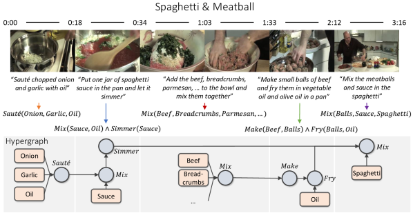
Figure 1: Representing a video instruction of making spaghetti $\&$ meatball with temporal hypergraph.

We summarize our contributions as follows:

• We propose temporal hypergraph, a graph that supports n-ary relations and temporal events with time intervals. We showcase that this is a natural and expressive representation for many applications.

• We propose a backward-chaining ILP method for the temporal hypergraph, which learns to generalize on both temporal and relational data. This is realized with a novel random B-walk algorithm and a time constraint propagation algorithm.

• We showcase our framework by creating two temporal hypergraph datasets from the YouCook2 cooking recipe dataset (Zhou et al., 2018) and nuScenes autonomous driving dataset (Caesar et al., 2020) and demonstrating the effectiveness of the proposed ILP method.

To the best of our knowledge, the temporal inductive logic reasoning (TILR) is the first framework that addresses the ILP problem on hypergraphs with time interval labels.

2 Related Work

ILP methods. Many ILP methods are proposed for inductive logic reasoning on graphs. These methods are categorized into two types. Forward-chaining methods (Galárraga et al., 2015; Evans and Grefenstette, 2018; Payani and Fekri, 2019) learn by searching in the rule space. It supports inferring difficult tasks but suffers from exponential complexity and does not scale to large graphs. On the other hand, backward-chaining methods (Campero et al., 2018; Yang and Song, 2020; Yang et al., 2017) learn rules by searching in the graph space, while the rule is usually limited to a chain-like path in the graph, this leads to better scalability. For temporal hypergraphs, none of the existing ILP methods are readily applicable. In this work, we propose the ILP method for temporal hypergraphs under the backward-chaining paradigm.

Temporal reasoning There are many ways for reasoning on temporal data. Some temporal KGs have events with single time points. And some recent methods such as TLogic (Liu et al., 2022) were proposed for solving ILP on these graphs. However, time point algebra is limited as it cannot represent temporal relations of events with duration. A more expressive representation is proposed in time interval algebra with Allen’s interval algebra (Allen, 1983) being the representative schema. In this work, we show how to incorporate the algebra for learning temporal relations.

3 Temporal Hypergraph and ILP

For an ordinary graph, is can be represented by a set of triples of the form $P(x_{h},x_{t})$, where $P$ is the predicate and $x_{h}$ and $x_{t}$ are the head and tail entities. To represent more complex structures with n-ary relations (i.e., relations that have arity greater than 2) and timestamps. We need to introduce the temporal hypergraph.

A temporal hypergraph consists of the following components: Entities: $x\in{\mathcal{X}}$ is the unique entity in the temporal data. Definitions. Predicate: $P\in{\mathcal{P}}$ is the temporal predicate. Event: an event is defined as ${\mathbf{e}}=P\left({\bm{x}}_{h},{\bm{x}}_{t},{\bm{t}}\right)$, where ${\bm{x}}_{h},{\bm{x}}_{t}$ are the head entities and tail entities, and ${\bm{t}}=\langle t_{s},t_{e}\rangle$ consists of the start and end time of an event. Therefore, a temporal hypergraph is defined as ${\mathcal{G}}=\langle{\mathcal{X}},{\mathcal{P}},{\mathcal{E}}\rangle$, where ${\mathcal{E}}=\{{\mathbf{e}}_{1},...,{\mathbf{e}}_{n}\}$ is a collection of events.

3.1 First-Order Logic

Given a graph, one can express knowledge as first-order logic (FOL) rules. A FOL rule consists of (i) a set of predicates defined in ${\mathcal{P}}$, (ii) a set of logical variables such as $X$ and $Y$, and (iii) logical operations $\{\land,\lor,\neg\}$. For example,

$$\texttt{GrandFatherOf}(X,X^{\prime})\leftarrow \texttt{FatherOf}(X,Y)\land$$ (1)

$$\texttt{MotherOf}(Y,X^{\prime})$$

involves predicates GrandFatherOf, FatherOf and MotherOf. Components such as $\texttt{FatherOf}(X,Y)$ are called atoms which correspond to the predicates that apply to the logical variables. Each atom can be seen as a lambda function with its logical variables as input. This function can be evaluated by instantiating the logical variables such as $X$ into the object in ${\mathcal{X}}$. For example, let ${\mathcal{X}}=\{\text{Amy},\text{Bob},\text{Charlie}\}$, we can evaluate $\texttt{FatherOf}(\text{Bob}/X,\text{Amy}/Y)$ by instantiating $X$ and $Y$ into Bob and Amy respectively. This yields 1 (i.e. True) if “Bob is the father of Amy”. The outputs of all atoms are combined using logical operations $\{\land,\lor,\neg\}$ and the imply operation $p\leftarrow q$ is equivalent to $p\lor\neg q$. Thus, when all variables are instantiated, the rule will produce an output as the specified combinations of those from the atoms. By using the logical variables, the rule encodes the “lifted” knowledge that does not depend on the specific data. Such representation is beneficial because (i) the rules are highly interpretable and can be translated into natural language for human assessment, and (ii) the rules guarantee to generalize to many examples.

3.2 Temporal Inductive Logic Reasoning

The Temporal Inductive Logic Reasoning (TILR) concerns solving the ILP problem for temporal data. Specifically, given a set of positive and negative queries ${\mathcal{Q}}_{+}$ and ${\mathcal{Q}}_{-}$, TILR learns the logic rules that predict (or entail) positive ones and do not predict the negative ones.

For example, one wants to summarize a recipe of making Spaghetti $\&$ Meatball from a set of videos $video_{1},...,video_{n}$ similar to Figure 1. Let ${\mathcal{G}}_{1},...,{\mathcal{G}}_{n}$ be the temporal graphs of the videos, then, this tasks corresponds to learning a logic rule that successfully predict the positive video labels ${\mathcal{Q}}_{+}=\{S\&M(video_{1}),...,S\&M(video_{n})\}$ and does not predict the negative video labels ${\mathcal{Q}}_{-}=\{S\&M(video_{i})|i\neq 1,...,n\}$.

Similarly, one can perform standard deductive reasoning on the graph, that is, link prediction or graph completion. In this case, positive queries consist of a set of events ${\mathcal{Q}}_{+}=\{{\mathbf{e}}_{1},...,{\mathbf{e}}_{n}\}$ (or triples, if ${\mathcal{G}}$ is a traditional KG), and the negative queries consist of another set of events. The task is to learn a set of rules that predict positive events and not negative events.

There are many ways to solve ILP. One can learn a logic program consisting of multiple rules, where by applying them repeatedly to the graph, the positive queries will be entailed (and the opposite for the negative ones). This is referred to as forward-chaining method (Campero et al., 2018; Evans and Grefenstette, 2018). On the other hand, one can solve each query independently, where a logic rule is proposed to predict a given query. This is referred to as backward-chaining method (Yang et al., 2017; Yang and Song, 2020). In other words, one learns a function $f(q;{\mathcal{G}})$ that maps a query $q$ into a logic rule. In this work, we consider the backward-chaining approach.

Definition 3.1 (Temporal Inductive Logic Reasoning)

Given a temporal hypergraph ${\mathcal{G}}$, and a set of positive and negative queries ${\mathcal{Q}}_{+}$ and ${\mathcal{Q}}_{-}$, find a model $f(q;{\mathcal{G}})$ that maps the query $q$ into a logic rule $R$ such that

$$R(q)=\mathds{1}[q\in{\mathcal{Q}}_{+}],\;\text{for}\;q\in{\mathcal{Q}}_{+}\cup{\mathcal{Q}}_{-}.$$

4 Proposed Method

Graph random walk is employed in many backward-chaining methods on traditional KG. Given a triple query $P(x_{h},x_{t})$, one searches a path from $x_{h}$ to $x_{t}$, which can be represented as a chain-like rule

$$P(x_{h},x_{t})\leftarrow P^{(1)}(x_{h},x^{(1)})\land P^{(2)}(x^{(1)},x^{(2)})\land...\land P^{(n)}(x^{(n)},x_{t}).$$

For temporal hypergraph with events $P\left({\bm{x}}_{h},{\bm{x}}_{t},{\bm{t}}\right)$, we need to address two challenges: 1) How to perform random walk on hypergraph?; and 2) How to incorporate the temporal relation while walking on the graph? We discuss these issues in this section.

Init: rule queue $q=\{s\}$, edge counter $\forall e\in{\mathcal{E}},k[e]=0$, probability $\forall x\in{\mathcal{X}},t=1...T,p[x][t]=0$, length $t=0$

while $q$ is not empty do

       $x=q.dequeue()$

      $t+=1$

      Child probabilities $childProb=[]$

      for $e\in UnvisitedEdgeFrom(x)$ do

            

            $k[e].add(x)$

            // visit $e$ if all tail vertices of $e$ are visited

            

            if $k[e]==T(e)$ then

                  

                  Mark $e$ as visited

                  $x^{\prime}=H(e)$ // because it’s B-Graph

                  

                  $p[x^{\prime}][t]+=\frac{1}{OutDegree(T(e))}\min_{x^{\prime\prime}\in T(e)}p[x^{\prime\prime}][t-1]$

                  $q.enqueue(x^{\prime})$

                  $childProb.append(p[x^{\prime}][t])$

             end if

            

       end for

      

end while

Algorithm 1 Multi-start Random B-walk

4.1 Reasoning via multi-start random B-walk

Many random walk techniques have been proposed for hypergraphs. For In (Chitra and Raphael, 2019), a fixed weight RW method is proposed. In (Chitra and Raphael, 2019), an edge-dependent vertex weight RW is proposed. There are also RW with nonlinear operators proposed to preserve properties of the RW on ordinary graphs(Chan et al., 2018; Li et al., 2020). However, none of the existing work is designed for ILP and concerns the important property, that is, the B-connectivity. In this work, we propose a novel RW method namely, the multi-start random B-walk (MRBW).

B-connectivity Consider a n-ary relation in the recipe example in Figure 1, that is, $\texttt{Mix}({\bm{x}}_{h},{\bm{x}}_{t},{\bm{t}})$, where ${\bm{x}}_{h}$ denotes the ingredients and ${\bm{x}}_{t}$ denotes the mixed output (therefore, in this case, $\text{dim}({\bm{x}}_{t})=1$). Let ${\bm{x}}^{(t)}$ be the set of nodes that are reached at $(t)$th step in a walk. Then, it is natural to say that “${\bm{x}}^{(t)}$ is connected to ${\bm{x}}_{t}$ by Mix if and only if ${\bm{x}}_{h}\subseteq{\bm{x}}^{(t)}$”. In other words, the tail nodes cannot be reached until all the head nodes are reached.

This property is referred to as B-connectivity (Gallo et al., 1993). Formally, let $P({\bm{x}}_{h},{\bm{x}}_{t},{\bm{t}})$ be a hyperedge of predicate $P$. Then, a hyperedge is a B-edge if $\text{dim}({\bm{x}}_{h})\geq 1$ and $\text{dim}({\bm{x}}_{t})=1$. In other words, $P$ is a many-to-one relation. And a path is B-connected if all of its B-edges are B-connected. A hypergraph consisting of only B-edges is called a B-graph. In this work, we consider the random walk on B-graphs.

Multi-start Random B-walk. For the traditional random walk, one starts from a node $x_{h}$ and randomly transits to the tail nodes with equal probability. In MRBW, we consider starting from a set of nodes, and random walking on the graph while maintaining the B-connectivity.

Let ${\bm{x}}^{(t-1)}$ be the nodes reached at $(t-1)$th step and ${\mathbf{X}}^{(t-1)}$ be the union of nodes from $(0)$ to $(t-1)$, and $P^{(t)}$ be the type of hyperedge by which transition is performed at $(t)$th step. For $\forall{\bm{x}}_{t}^{(t)}\subseteq{\mathcal{X}}$ that are reachable at $(t)$th step We have

$$p({\bm{x}}_{t}^{(t)})=\sum_{{\bm{x}}_{h}\in{\mathbf{X}}^{(t-1)}}\min_{x_{h}\in{\bm{x}}_{h}}\frac{1}{\text{OutDegree}(x_{h})}p(x_{h}^{(t-1)})$$

4.2 Temporal relations

So far we have been discussing how to address the random walk with n-ary relations. Here, we consider how to integrate the temporal relations introduced in (Allen, 1983) into the random walk, e.g., BEFORE, EQUAL, MEETS and etc. Instead of treating temporal relations as a separate operation from conjunction $\land$. we consider them as composite conjunction of the following form

$$P({\bm{x}}_{h},{\bm{x}}_{t},{\bm{t}})\;\texttt{BIN}\;P^{\prime}({\bm{x}}_{h}^{\prime},{\bm{x}}_{t}^{\prime},{\bm{t}}^{\prime})=\Big{(}P\left({\bm{x}}_{h},{\bm{x}}_{t}\right)\land P^{\prime}\left({\bm{x}}_{h}^{\prime},{\bm{x}}_{t}^{\prime}\right)\Big{)}\land\Big{(}\texttt{BIN}\left({\bm{t}},{\bm{t}}^{\prime}\right)\Big{)},$$

where $\texttt{BIN}\in\{\texttt{BEFORE},\texttt{EQUAL},\texttt{MEETS},...\}$. In order to generalize the temporal relations from the data, one keeps track of the set of applicable temporal relations for each pair of the events in the rule. Whenever a positive query is matched by the rule, one updates the temporal relations to satisfy the time constraints posed in the corresponding subgraph of the query. This is the traditional path-consistency (PC) algorithm introduced in (Allen, 1983). In this work, we incorporate the PC algorithm and propose the modified PC for MRBW. The algorithm is shown Algorithm 2. Here, $ResolveTime$ is the standard PC algorithm. Intuitively, the modified PC algorithm resolves time constraints whenever the two random walk paths merges together. This way, one does not need to update the relations at each step of the random walk, because the events within each path is already ordered.

Init: Path set $P=\{x_{1},x_{2},...\}$, $TimeOP[p_{i}][p_{j}]=0,\forall p_{i},p_{j}\in{\mathcal{G}}$, max search depth $D$

while $maxLen(P)<D$ do

       ${\mathcal{X}}_{heads}=HeadsOf(P)$

      $e\sim UnvisitedEdgeFrom({\mathcal{X}}_{heads})$

      if $e$ is B-connected then

             $P^{\prime}\leftarrow PathsEndWith(HeadsOf(e))$

            for $\{p_{i},p_{j}\}\in P`\times P^{\prime}$ do

                   $TimeOP[p_{i}][p_{j}]=ResolveTime(p_{i},p_{j})$

             end for

            

            for $p_{i}\in P`$ do

                   $TimeOP[e][p_{j}]=ResolveTime(e,p_{j})$

             end for

            

            $p^{*}\leftarrow BuildPath(e,P^{\prime},TimeOP)$

            $P/P`;P\cup\{p^{*}\}$

       end if

      

      return $P$

end while

Algorithm 2 Path-consistency for temporal relation generalization.

5 Learning

By applying the MRBW and the PC algorithm, one can develop many ILP methods that learn temporal logic rules from the data. Here, we propose a simplistic approach that follows the setup introduced in (Lao et al., 2011) that learns a linear model to weigh the paths in answering the query.

Let $R_{1},...,R_{n}$ be the $n$ candidate rules for reasoning. We define a linear model that predicts the score of answering the query $q={\bm{e}}=P({\bm{x}}_{h},{\bm{x}}_{t},{\bm{t}})$, that is

$$f_{\bm{\theta}}({\bm{e}};{\mathcal{G}})=\sum_{i}\theta_{i}R_{i}({\bm{x}}_{h},{\bm{x}}_{t},{\bm{t}}),$$

where $\theta_{1},...,\theta_{n}$ are the learnable parameters. Then the parameters can be learned by optimizing a cross-entropy loss

$$L(\bm{\theta};{\mathcal{G}})=\sum_{j}^{N}y_{i}logf_{\bm{\theta}}({\bm{e}}_{i};{\mathcal{G}})+(1-y_{i})log(1-f_{\bm{\theta}}({\bm{e}}_{i};{\mathcal{G}})),$$

where $N$ is the number of training queries, and $y_{i}\in{0,1}$ is the binary label indicating if the query is positive.

6 Experiment

6.1 Recipe summarization

YouCook2 cooking recipe dataset (Zhou et al., 2018) consists of instructional videos of 89 cooking recipes such as spaghetti $\&$ meatballs. Each recipe has 22 videos and each video is annotated by a sequence of natural language sentences that describe the procedure steps, as shown in Figure 1.

The dataset serves as a challenging benchmark for evaluating the generalizability of both temporal and relational data. To see this, instructions belonging to the same class can have different procedures and varied ingredients. For example, one can make BLT sandwich by first putting the lettuce on the bread and then the ham, or in the reserve order. This requires the ILP method to learn generalized temporal relations for the temporal events. On the other hand, instructions can differ by the actual steps and ingredients used. For example, some instructions of BLT sandwich involve mayonnaise while others do not. This requires the ILP method to learn rules that generalize these patterns.

Table 1: Statistics of the temporal hypergraph benchmark based on the YouCook2 recipe instructions.

Predicate Type		# Predicates	# Facts		Examples
			Per Graph	Total
Relation	Unary	208	58	10426	Cut, fry
	Binary	51	29	5213	Put
	N-ary	1	69	12417	MixInto
Class		1136	257	45881	Oil, Oinon, Noodle

Hypergraph construction. We construct the temporal hypergraph from the instruction sentences. For each clip, we run NLTK tools and extract the nouns and verbs from the sentences. We collect verbs as temporal relations. After pre-processing and grouping synonyms, there are 208 unary relations, 51 binary relations, and 1 n-ary relation. There are many possible n-ary relations in the raw data that describe the similar action, such as “put together” and “stir together”. Given the low frequency of each data, we consider merging them into a single n-ary relation, that is MixInto. Statistics are shown in Table 1.

Additionally, we create another version of the dataset with ordinary graphs and time point labels. This is done by: 1) converting the hypergraph via clique-expansion; 2) dropping the end time of the time intervals and treating the start time as the time point label.

Task. The goal of recipe summarization is to generalize a structured procedure for each distinct recipe from the hypergraph data. Formally, Let $({\mathcal{G}},y)$ be a hypergraph and its recipe type label (e.g. BLT sandwich). Let $y^{*}$ be the target type for which we want to summarize; the background, positive and negative sets of $y^{*}$ are

$${\mathcal{Q}}_{+}=\{({\mathcal{G}},y)|y=y^{*}\}, {\mathcal{Q}}_{-}=\{({\mathcal{G}},y)|y\neq y^{*}\}.$$ (2)

The positive set is essentially the set of positive hypergraphs, as the task is to learn rules from the hypergraph which can entail the positive hypergraphs of recipe $y^{*}$ and do not entail the negative ones. Since the goal is to generate

However, Eq.(2) is not sufficient for generating rules for summarization. Without additional constraints Eq.(2) essentially becomes a graph classification task, and solving it can lead to rules with good accuracy but poor interpretability. For examples, one can learn rules that classify spaghetti $\&$ meatballs easily by solely checking if the Spaghetti and Meatball class labels are present in the graph. To solve this, we put the constraint that the rules must cover most of the time span of the target hypergraphs. In other words, it needs to find rules that generalize to a significant subgraph in the hypergraph. This can be done by keeping track of the earliest and the latest events when a subgraph is matched by a rule. If the duration of the subgraph is less than that of the entire graph then the rule is discarded.

Methods. We evaluate three versions of our ILP method: 1) MRBW: this version performs vanilla MRBW without the path-consistency (PC) algorithm; it proposes the best rule for each recipe by counting the occurrences and picking the most frequent one. 2) MRBW+PC: this version is the same as MRBW but with PC algorithm. 3) MRBW+PC (train): this version performs MRBW and PC algorithm during search and learns rule via the parametric model introduced in section 5.

We also compare with methods of two categories: 1) GNN-GCN (Kipf and Welling, 2016) and GNN-Cheb Defferrard et al. (2016). GNN methods use the clique-expansion graph and ignores the time labels. The goal for including neural models is to provide a reference for score comparison: the neural models treat the task as a graph classification task; they do not produce interpretable results, but they tend to outperform the symbolic and neuro-symbolic counterparts. 2) CTDNE (Nguyen et al., 2018). A graph embedding methods that utilize the time point labels in clique-expansion graph. 3) random walk (RW) and NeuralLP (Yang et al., 2017). These are two ILP methods via counting and differentiable learning respectively. We implement the RW method as a simplistic baseline that performs personalized random walks (that is starting from the given start point) on the clique-expansion graph while ignoring the time labels; it counts the frequency of paths that answer the query. All experiments are done on a PC with i7-8700K and one GTX1080ti. We use the Mean Reciprocal Rank (MRR) and Hits@3 (H@3) and Hits@10 (H@10) as the metrics,

Table 2: MRR and Hits of three MRBW methods on recipe summarization task together with that of three GNN-based methods and two static graph ILP methods.

Method	Clique-Expansion			Hypergraph
	MRR	H@3	H@10	MRR	H@3	H@10
GNN-GCN	0.76	79.2	82.1	-	-	-
GNN-Cheb	0.78	80.7	82.9	-	-	-
CTDNE	0.81	85.3	87.6	-	-	-
RW	0.19	18.8	20.6	-	-	-
NeuralLP	0.36	37.1	39.5	-	-	-
MRBW	0.25	20.4	23.7	0.35	29.4	36.3
MRBW+PC	0.30	27.9	31.1	0.60	55.8	59.1
MRBW+PC (train)	0.42	38.2	42.5	0.72	76.0	79.4

Results. The results are shown in Table 2, For clique-expansion graph, the three GNN-based methods achieved the best performance. By inspecting the data (Appendix B), we found that the class labels in the hypergraph are highly correlated with the recipe types. For example, Lettuce and Ham frequently co-occur with BLT; and Wasabi co-occurs with Salmon Sashimi. This suggests the GNN-based models have learned to rely on this information to classify the graph. On the other hand, for the ILP methods with the constraint that filters out the trivial rules, the scores are lower. The first two versions of MRBW obtain a comparative score with the ILP baselines and the trained MRBW achieves the best performance within the ILP category.

For the temporal hypergraph representation, only MRBW is applicable. And the performance of the three versions of the method improves significantly. This suggests the hypergraph representation retains useful higher-order information and our MRBW is capable of learning it.

6.2 Driving behavior explanation

Table 3: Statistics of the temporal hypergraph benchmark based on the nuScenes autonomous driving datasets.

Predicate Type		# Predicates	# Facts		Examples
			Per Graph	Total
Relation	Unary	13	4631	3473257	ego.throttle
					ego.brake
	Binary	6	1859	1394253	in_front
					behind
	N-ary	1	1692	1269004	Between
Class		23	257	45881	vehicle.car
					human.pedestrian.adult
					ped_crossing

Figure 2: Example driving logs in nuScenes.

The nuScenes autonomous driving dataset (Caesar et al., 2020) consists of 750 driving scenes in the training set (Figure 2). Each scene is a 20s video clip; each frame in the clip is annotated with 2D bounding boxes and class labels. The dataset also provides the lidar and ego information such as absolute position, brake, throttle, and acceleration.

Hypergraph construction. We construct the temporal hypergraph for each driving scene. For class labels, we use the provided 23 object classes, including vehicle.car and human.pedestrian.adult. For the predicate, the ego information together with the object attribute such as vehicle.moving and pedestrian.moving are considered the unary predicates. The original dataset does not provide relations for the objects. Here, we create the relative spatial relations by inferring from the absolute spatial information. This includes In_front, Behind, Between and etc. The statistics are shown in Table 3.

Task. We apply TILR to explain the driving behavior with temporal logic rules. Such explanation is beneficial as it can provide insight of why certain behavior happens, for example, one can explain that in what situation will the driver hit the brake; the evidence is likely to be there is a pedestrian crossing the street. Formally, we consider the positive queries to be the events of ego.brake and ego.throttle and the rest of the events are the negative queries, that is

$${\mathcal{Q}}_{+}=\{P({\bm{x}}_{h},{\bm{x}}_{t},{\bm{t}})|P\in\{\texttt{ego.brake},\texttt{ego.throttle}\}\},$$

$${\mathcal{Q}}_{-}=\{P({\bm{x}}_{h},{\bm{x}}_{t},{\bm{t}})|P\notin\{\texttt{ego.brake},\texttt{ego.throttle}\}\}.$$

Table 4: MRR and Hits of the three versions of MRBW on the nuScenes hypergraph benchmark.

Method	nuScenes Hypergraph
	MRR	H@3	H@10
MRBW	0.19	20.8	31.4
MRBW+PC	0.22	24.1	35.5
MRBW+PC (train)	0.46	45.3	52.7

Similar to the recipe summarization. We evaluate three versions of our ILP method: MRBW, MRBW+PC, and MRBW+PC (train).

Results. The results are shown in Table 4. The results suggest that the gap between the trained and untrained version of the MRBW are more significant in this benchmark. This is because the driving scenes are more diverse and many situations can lead to the target event. This makes it difficult to learn rules by counting and picking the best one. In this case, a learned model that proposes the rule for individual scenes yields a higher score.

7 Conclusion

In this work, we propose temporal inductive logic reasoning (TILR). A novel framework that extends the ILP technique to applications beyond knowledge graphs. We first introduce the temporal hypergraph and show that this is a powerful representation for many applications; we then propose the multi-start random B-walk (MRBW) algorithm that serves as the foundation of developing ILP methods on this hypergraph. Finally, we propose an ILP method based on MRBW and a path-consistency algorithm that generalizes on both the temporal and the relational data. The TILR is evaluated on the YouCook2 and nuScenes datasets and demonstrates strong performance.

Appendix A Temporal KG completion

Table 5: MRR and Hits of MSWR on three temporal KG datasets together with baseline methods of two categories.

Method	ICEWS14			ICEWS18			GDELT
	MRR	H@3	H@10	MRR	H@3	H@10	MRR	H@3	H@10
DistMult	0.19	22.0	36.4	0.22	26.0	42.2	0.19	20.1	32.6
RotatE	0.30	32.9	42.7	0.23	27.6	38.7	0.22	23.9	32.3
TA-DistMult	0.21	22.8	35.3	0.29	31.6	45.0	0.29	31.6	41.4
RE-NET	0.46	49.1	59.1	0.43	45.5	55.8	0.40	43.4	53.7
TLogic	0.43	48.3	61.2	0.30	33.95	48.53	-	-	-
MRBW	0.32	36.1	50.3	0.31	33.1	46.8	0.34	37.5	45.6

The proposed multi-start random B-walk (MRBW) is also applicable to the Temporal KG datasets. We evaluate it on the ICEWS [Boschee et al., 2015] and the GDELT [Leetaru and Schrodt, 2013] datasets.

The temporal KG dataset consists of snapshots of graphs for a series of time points. To apply MRBW, we modify the graph as followings: 1) we change time point labels into time intervals with the same start and end time; and 2) we add edges s $\texttt{IsSameEnt}(x,x^{\prime},{\bm{t}})$ to the graphs. The edge connects the entities of the same IDs in the temporal KGs with start and end time match the time points of the two connected graph snapshots. As the original graphs at different time points are disconnected, these edges essentially create paths that go across different time points. Note that we keep the conversion minimal and avoid introducing additional information into the graph for a fair comparison. The goal of this study is not to propose a state-of-the-art reasoning method for temporal KGs, as the MRBW is not designed for this dataset. Instead, this serves as a sanity check on how the algorithm performs on the common benchmarks.

We evaluate MRBW together with baselines of two categories on the link forecasting task defined in [Liu et al., 2022]. We used the data split provided in [Jin et al., 2019]. The results are shown in Table 5; baseline results are taken from [Liu et al., 2022, Jin et al., 2019]. The results suggest that MRBW has comparable performance with the popular static and temporal graph reasoning models. To improve the performance, one can introduce a parametric model for rule learning just as that in section 5. We leave this investigation in future work.

Appendix B Example hypergraphs

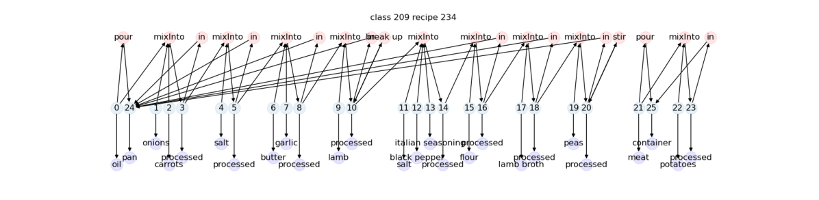
Figure 3: Example temporal hypergraph for recipe Shepherd’s Pie.

References

- Allen [1983] James F Allen. Maintaining knowledge about temporal intervals. Communications of the ACM, 26(11):832–843, 1983.
- Bordes et al. [2013] Antoine Bordes, Nicolas Usunier, Alberto Garcia-Duran, Jason Weston, and Oksana Yakhnenko. Translating embeddings for modeling multi-relational data. In Advances in neural information processing systems, pages 2787–2795, 2013.
- Boschee et al. [2015] Elizabeth Boschee, Jennifer Lautenschlager, Sean O’Brien, Steve Shellman, James Starz, and Michael Ward. ICEWS Coded Event Data, 2015. URL https://doi.org/10.7910/DVN/28075.
- Caesar et al. [2020] Holger Caesar, Varun Bankiti, Alex H. Lang, Sourabh Vora, Venice Erin Liong, Qiang Xu, Anush Krishnan, Yu Pan, Giancarlo Baldan, and Oscar Beijbom. nuscenes: A multimodal dataset for autonomous driving. In CVPR, 2020.
- Campero et al. [2018] Andres Campero, Aldo Pareja, Tim Klinger, Josh Tenenbaum, and Sebastian Riedel. Logical rule induction and theory learning using neural theorem proving. arXiv preprint arXiv:1809.02193, 2018.
- Chan et al. [2018] T-H Hubert Chan, Anand Louis, Zhihao Gavin Tang, and Chenzi Zhang. Spectral properties of hypergraph laplacian and approximation algorithms. Journal of the ACM (JACM), 65(3):1–48, 2018.
- Chitra and Raphael [2019] Uthsav Chitra and Benjamin Raphael. Random walks on hypergraphs with edge-dependent vertex weights. In International Conference on Machine Learning, pages 1172–1181. PMLR, 2019.
- Defferrard et al. [2016] Michaël Defferrard, Xavier Bresson, and Pierre Vandergheynst. Convolutional neural networks on graphs with fast localized spectral filtering. Advances in neural information processing systems, 29, 2016.
- Evans and Grefenstette [2018] Richard Evans and Edward Grefenstette. Learning explanatory rules from noisy data. Journal of Artificial Intelligence Research, 61:1–64, 2018.
- Galárraga et al. [2015] Luis Galárraga, Christina Teflioudi, Katja Hose, and Fabian M Suchanek. Fast rule mining in ontological knowledge bases with amie+. The VLDB Journal—The International Journal on Very Large Data Bases, 24(6):707–730, 2015.
- Gallo et al. [1993] Giorgio Gallo, Giustino Longo, Stefano Pallottino, and Sang Nguyen. Directed hypergraphs and applications. Discrete applied mathematics, 42(2-3):177–201, 1993.
- Jin et al. [2019] Woojeong Jin, Meng Qu, Xisen Jin, and Xiang Ren. Recurrent event network: Autoregressive structure inference over temporal knowledge graphs. arXiv preprint arXiv:1904.05530, 2019.
- Kipf and Welling [2016] Thomas N Kipf and Max Welling. Semi-supervised classification with graph convolutional networks. arXiv preprint arXiv:1609.02907, 2016.
- Lao et al. [2011] Ni Lao, Tom Mitchell, and William Cohen. Random walk inference and learning in a large scale knowledge base. In Proceedings of the 2011 conference on empirical methods in natural language processing, pages 529–539, 2011.
- Leetaru and Schrodt [2013] Kalev Leetaru and Philip A Schrodt. Gdelt: Global data on events, location, and tone, 1979–2012. In ISA annual convention, volume 2, pages 1–49. Citeseer, 2013.
- Li et al. [2020] Pan Li, Niao He, and Olgica Milenkovic. Quadratic decomposable submodular function minimization: Theory and practice. J. Mach. Learn. Res., 21:106–1, 2020.
- Liu et al. [2022] Yushan Liu, Yunpu Ma, Marcel Hildebrandt, Mitchell Joblin, and Volker Tresp. Tlogic: Temporal logical rules for explainable link forecasting on temporal knowledge graphs. arXiv preprint arXiv:2112.08025, 2022.
- Nguyen et al. [2018] Giang Hoang Nguyen, John Boaz Lee, Ryan A Rossi, Nesreen K Ahmed, Eunyee Koh, and Sungchul Kim. Continuous-time dynamic network embeddings. In Companion Proceedings of the The Web Conference 2018, pages 969–976, 2018.
- Payani and Fekri [2019] Ali Payani and Faramarz Fekri. Inductive logic programming via differentiable deep neural logic networks. arXiv preprint arXiv:1906.03523, 2019.
- Toutanova and Chen [2015] Kristina Toutanova and Danqi Chen. Observed versus latent features for knowledge base and text inference. In Proceedings of the 3rd Workshop on Continuous Vector Space Models and their Compositionality, pages 57–66, 2015.
- Yang et al. [2017] Fan Yang, Zhilin Yang, and William W Cohen. Differentiable learning of logical rules for knowledge base reasoning. In Advances in Neural Information Processing Systems, pages 2319–2328, 2017.
- Yang and Song [2020] Yuan Yang and Le Song. Learn to explain efficiently via neural logic inductive learning. In International Conference on Learning Representations, 2020. URL https://openreview.net/forum?id=SJlh8CEYDB.
- Zhou et al. [2018] Luowei Zhou, Chenliang Xu, and Jason J Corso. Towards automatic learning of procedures from web instructional videos. In AAAI Conference on Artificial Intelligence, pages 7590–7598, 2018. URL https://www.aaai.org/ocs/index.php/AAAI/AAAI18/paper/view/17344.