A GPU-Accelerated Light-field Super-resolution Framework Based on Mixed Noise Model and Weighted Regularization

Abstract

Light-field (LF) super-resolution (SR) plays an essential role in alleviating the current technology challenge in the acquisition of a 4D LF, which assembles both high-density angular and spatial information. Due to the algorithm complexity and data-intensive property of LF images, LFSR demands a significant computational effort and results in a long CPU processing time. This paper presents a GPU-accelerated computational framework for reconstructing high resolution (HR) LF images under a mixed Gaussian-Impulse noise condition. The main focus is on developing a high-performance approach considering processing speed and reconstruction quality. From a statistical perspective, we derive a joint $\ell^{1}$-$\ell^{2}$ data fidelity term for penalizing the HR reconstruction error taking into account the mixed noise situation. For regularization, we employ the weighted non-local total variation approach, which allows us to effectively realize LF image prior through a proper weighting scheme. We show that the alternating direction method of multipliers algorithm (ADMM) can be used to simplify the computation complexity and results in a high-performance parallel computation on the GPU Platform. An extensive experiment is conducted on both synthetic 4D LF dataset and natural image dataset to validate the proposed SR model’s robustness and evaluate the accelerated optimizer’s performance. The experimental results show that our approach achieves better reconstruction quality under severe mixed-noise conditions as compared to the state-of-the-art approaches. In addition, the proposed approach overcomes the limitation of the previous work in handling large-scale SR tasks. While fitting within a single off-the-shelf GPU, the proposed accelerator provides an average speedup of 2.46${\mkern-2.0mu\times\mkern-2.0mu}$ and 1.57${\mkern-2.0mu\times\mkern-2.0mu}$ for ${\mkern-2.0mu\times\mkern-2.0mu}2$ and ${\mkern-2.0mu\times\mkern-2.0mu}3$ SR tasks, respectively. In addition, a speedup of $77{\mkern-2.0mu\times\mkern-2.0mu}$ is achieved as compared to CPU execution.

1 Introduction

Light field (LF) refers to the concept of capturing a comprehensive description of light rays. Although a complete parameterization of LF would require a 7D plenoptic function Adelson1992single , practical applications have been successfully made use of its simplified 4D version Levoy1996light . Among four dimensions, two dimensions are for perspective indexing, and the other dimensions assemble the spatial information, see Fig. 1. The rich-content property of LF brings a great advantage to numerous applications such as in autonomous systems Silva2021light , virtual reality Overbeck2018system , 3D television Ni2018360 . However, this benefit also comes with a cost of computational resources. Processing 4D LF images requires more memory bandwidth, computing power and runtime than the conventional 2D image. This problem encourages the use of Graphics Processing Unit (GPU) for offloading LF image processing tasks. There are three main techniques to capture 4D LF data: time-sequential Unger2003capturing , multi-sensors Wilburn2005high , and multiplexing Adelson1992single . These acquisition methods compromise between spatial resolution and angular or temporal resolution, i.e., using a low-resolution imaging sensor to reduce cost while increasing the number of cameras for a higher angular resolution Wilburn2005high ; moving camera with more spatial steps to capture more perspective images but suffering from a long acquisition time Unger2003capturing ; Increasing the number of microlenses for a higher spatial resolution while reducing the angular resolution Adelson1992single . These existing challenges in high-resolution LF acquisition are driving recent research on super LF resolution (LFSR) Cheng2019light .

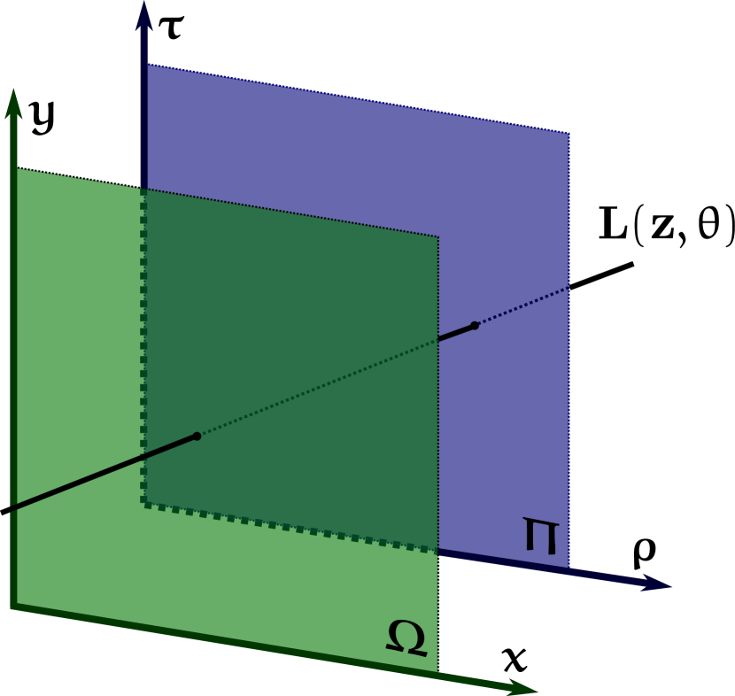
(a)

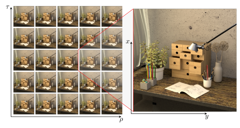
(b)

Figure 1: Light-field representation and acquisition; (a) Two-plane parameterisation; (b) 2D array representation of sub-aperture images (SAIs).

The super-resolution of LF image aims to reconstruct a high-resolution (HR) view, also referred to as sub-aperture image (SAI), from a 2D array of low-resolution (LR) views, see Fig. 1 (b). Many approaches have been proposed for the LFSR, including convolutional neural network (CNN) based approaches Yuan2018light ; Zhang2019residual ; Tran20223dvsr and optimization based approaches Bishop2012light ; Rossi2018geometry ; Alain2018light . Although providing high-quality SR results, these approaches typically comprise multiple processing stages and complex algorithms, leading to high computational demand and a long processing time. For example, multi-stage CNN-based approaches Yuan2018light ; Tran20223dvsr divide LFSR into two steps. The first step employs very deep and large CNNs Kim2016accurate ; Lim2017enhanced for separately up-scaling LR SAIs. Another refinement CNN is trained and applied in the second step for enhancing the quality of HR SAI. Other examples are Rossi2018geometry consisting of time-consuming graph processing tasks and Alain2018light involving computational demanding 5D filtering operator. As far as we know, the literature on GPU accelerated LFSR is very limited despite its importance. While focusing on the quality aspect, previous approaches put aside the run-time constraint and leave the possibility of accelerating SR tasks undiscussed.

This paper presents a GPU accelerated approach for 4D light-field image super-resolution. First, we proposed a computational framework for reconstructing high resolution sub-aperture images from 4D LF data, Sec. 3. The LF super-resolution model derived from the statistical perspective consists of a joint $\ell^{1}$-$\ell^{2}$ data fidelity term and a weighted nonlocal total variation regularization term. While the first term provides a proper treatment to mixed Gaussian-Impulse noise conditions, the second term introduces an effective way to integrate image features for a better regularization effect. A weighting scheme combining bilateral effect, edge and occlusion features is also proposed. Secondly, we show that the proposed optimization problem can be effectively solved with the alternating direction method of multipliers (ADMM), Sec. 4. ADMM resolves the main problem of steepest gradient descent in finding a proper step size while avoiding costly line-search operations. Third, a GPU accelerated architecture is presented for speeding up the iterative solver, Sec. 5. Through the realization of transformation matrices with linear functions, which are effectively realized in the form of GPU kernel execution, the proposed approach alleviates the resource shortage of sparse matrix implementation. As shown in the experimental result, the proposed approach can super-resolve large size images (i.e., up to 5760${\mkern-2.0mu\times\mkern-2.0mu}$5760) within a single GPU as compared to 4 GPUs used in the related work Sun2021fl . In Sec. 7 an extensive experiment is conducted on synthetic 4D LF dataset Honauer2016dataset ; Shi2019framework and natural image dataset DIV8K Gu2019div8k to validate the robustness of the proposed SR model and evaluate the performance of the accelerated computational framework. Through the OpenCL framework, the accelerated solver can be deployed on various GPU platforms bringing up a speed-up of 77${\mkern-2.0mu\times\mkern-2.0mu}$ as compared to CPU execution. The contribution of this work can be summarized as follows:

• Optimization-based approach for spatially SR of LF image under mixed Gaussian-Impulse noise condition assembling a joint $\ell^{1}-\ell^{2}$ data term with weighted nonlocal TV regularization term.

• Application of ADMM for solving the proposed optimization problem. As shown in Sec. 4, by properly rewriting the optimization problem into the form of ADMM, the solving process is simplified and more suitable for parallel implementation on the GPU platform.

• OpenCL-based acceleration of the iterative solving process. As discussed in Sec. 5 and 7, our accelerator not only provides a significant speed-up as compared to CPU but also overcomes the limitation of the previous work in handling large scale SR problems on the GPU platform.

2 Related Works

This section discusses the previous works on the super-resolution of 4D LF images, which are divided into two categories: optimization-based approach and learning-based approach. Among these two, learning-based approaches present state-of-the-art performance.

2.1 Optimization-based Methods

Optimization-based methods generally formulated LF SR as an optimization problem, including a data fidelity term built upon a degradation model and a regularization term based on an assumed prior. Regarding the data term, previous works proposed either penalizing the coherence between LR and HR sub-aperture images  Bishop2012light ; Alain2018light or enforcing the intensity similarity over the angular dimension by warping sub-aperture images Tran2018gpu ; Rossi2018geometry . Regarding the regularization term, the choice is more diverse. Many image priors are proposed to achieve better output quality and with reasonable computational cost, i.e. Markov Random Field (MRF) Bishop2012light , Bilateral TVTran2018gpu , graph-based Rossi2018geometry , sparsity Alain2018light .

In Bishop2012light , Bishop et al. formulated LF imaging process by a set of spatially-variant point spread functions (PSFs). Under Gaussian optic assumptions, these PSFs are derived and applied in a Bayesian SR framework. In Tran2018gpu , LFSR was studied in the context of a multi-image super-resolution problem which considers degradation process as a combination of three operators: warping, blurring and down-scaling. The authors employed a variational framework Tran2017variational to estimate disparity maps used for warping functions, while BTV was selected for regularization. In Rossi2018geometry , Rossi et al. assembled an optimization problem with a graph-based regularizer and two $\ell^{2}$ data terms. They employed block matching for estimating disparity values which was used to build the graph map. A patch-based SR approach was proposed in Alain2018light . The authors made used of a 5D transform filter consisting of 2D shape-adaptive DCT, 2D DCT transform, and 1D haar wavelet. By a proper selection of 5D patches, a high degree of sparsity was expected in the transformed signal. This sparsity property was employed for regularization in combination with a $\ell^{2}$ data term.

2.2 Deep Learning-based Approaches

Deep learning-based methods for LFSR are mainly categorized into two groups. While the first group directly exploits the multi-dimensional structure of LF in learning an end-to-end neural network to synthesize high-resolution view Yeung2018light ; Zhang2019residual , the second group employs a multi-stages processing model for a step-by-step improvement of the reconstruction quality Yuan2018light ; Tran20223dvsr . A 4D convolution method was proposed in Yeung2018light to fully exploit the 4D structure of LF images. The 4D convolution was realized as an angular-spatial separable convolution allowing the acquisition of feature maps from both angular and spatial domains. In Zhang2019residual , a residual CNN-based approach was proposed for the super-resolution of LF images. Their network was provided with stacking images from four different angles and predicted an HR image at the central perspective. Due to the diversity in directional position, six CNNs were needed for completely reconstructing high-resolution LF. Compared to learning a single SR network, the two-stages model provides more flexibility and potentially higher reconstruction quality. This type of approach takes advantage of well-trained single image super-resolution (SISR) networks Kim2016accurate ; Lim2017enhanced to separately reconstruct an HR view of each SAI in the first stage. These HR images are then enhanced in the second stage through a novel CNN which makes use of inter-perspective information across multiple SAIs. In Fan2017two , Fan et al. used VDSR Kim2016accurate in the first stage and applied a patch-based warping strategy to register the pre-scaling images. The registered images were combined with a reference image before feeding to the second-stage CNN for rendering the final HR view. Yuan et al. Yuan2018light employed EDSR Lim2017enhanced as SISR and proposed a refinement CNN which relies on 2D epipolar image for the second stage. Recently, Tran et al. Tran20223dvsr proposed an approach that exploits the 3D EPI structure of LF in a two-stages SR framework. Their method aimed for various LFSR problems, i.e., spatial, angular, and angular-spatial super-resolution. As compared to 2D EPI, which is limited to one spatial dimension, 3D EPI, which assembles two spatial dimensions along with one angular dimension, provides a significant contribution to enhance reconstruction quality. Departed from the usual strategy of employing CNN to directly enhance SR reconstruction quality, Guo et al. Guo2021deep proposed to learn coded aperture from LF data and used it as an implicit LF image prior to a deep learning-based framework for de-noising and reconstructing HR LF. Their approach, however, does not consider Impulse noise and treats de-noising and HR as separate reconstruction problems.

2.3 GPU Accelerated LF Processing

The high demand for computational resources due to the large amount of data provided with 4D LF image encourages the use of GPU as an acceleration platform. Recent works on GPU-based acceleration focus on two main LF processing tasks, disparity estimation Ivan2018light ; Tran2021gvld , and super-resolution Tran2018gpu . For disparity estimation, a GPU acceleration architecture was presented in Ivan2018light for cost-volume based optimization. The authors employed an advanced matching cost from Park2018robust but decided to choose the winner-take-all solution over the global minimum as scarification of accuracy for less complexity and computation. On the contrary, GVLD Tran2021gvld proposed a GPU-accelerated approach based on a variational computation framework. The framework combines the intrinsic sub-pixel precision of variational formulation and the effectiveness of weighted median filtering to produce a highly accurate solution. A fully parallelized and optimized OpenCL implementation was provided for finding the global minimum solution.

For super-resolution, Tran et al. Tran2018gpu proposed to accelerate the optimization problem which assembles an $\ell^{1}$ data fidelity term and a BTV Farsiu2004fast regularization term. Using steepest descent as an iterative solver, which is fully realized with OpenCL kernel execution, the proposed approach provides a significant speed-up as compared to the implementation running on CPU. This paper extends our previous work Tran2018gpu mainly as follows. First, we revisit the super-resolution model from the statistical perspective and propose a mixed noise (Gaussian and Impulse noise) model based on a combination of $\ell^{1}$ and $\ell^{2}$ fidelity terms. Secondly, we propose a nonlocal total variation weighting scheme that combines bilateral filtering with image features to improve the regularization effect. Thirdly, the alternating direction method of multipliers (ADMM) is employed in this work for solving the optimization problem as a replacement to the steepest descent. ADMM address the short-coming of the steepest descent in finding appropriate step-size while avoiding time-consuming line-search. Lastly, we present an accelerated architecture for realizing the computational framework on the GPU platform. The proposed approach is validated and evaluated through an extensive experiment on synthetic 4D LF dataset and high-resolution natural image dataset.

3 Proposed Approach

This section discusses our proposed approach for reconstructing high-resolution LF images under mixed noise conditions. The section starts with a presentation of the degradation model and notation, which form a basis for discussing the proposed optimization model derived from the Bayesian image reconstruction framework. Our selection of data fidelity term and regularization term are consecutively discussed at the end of this section.

3.1 Degradation Model and Notation

Light-field is a 4D parameterization of the plenoptic function Levoy1996light which can be illustrated as a light ray intersecting with two parallel planes,

$$\boldsymbol{L}\colon\Omega{\mkern-2.0mu\times\mkern-2.0mu}\Pi\rightarrow\mathbb{R},\qquad(\mathfrak{\textbf{z}},\boldsymbol{\theta})\rightarrow\boldsymbol{L}(\mathfrak{\textbf{z}},\boldsymbol{\theta}),$$ (3)

with $\boldsymbol{\theta}=[\rho,\tau]^{T}$ and $\mathfrak{\textbf{z}}=[x,y]^{T}$ indicate the coordinates in the directional plane $\Pi\subset\mathbb{R}^{2}$ and the spatial plane $\Omega\subset\mathbb{R}^{2}$, see Fig. 1(a). By fixing the directional coordinate $\boldsymbol{\theta}$ and let spatial coordinate z vary, we obtains the spatial information from one perspective. Such spatial information is referred to as a sub-aperture image (SAI) or a perspective image. Fig. 1(b) shows a $5{\mkern-2.0mu\times\mkern-2.0mu}5$ angular views of LF scene ‘table’ Honauer2016dataset . From this perspective, a 4D LF is a collection of 2D images captured from different viewpoints and the reconstruction of high-resolution SAIs shows a strong connection to the multi-image super-resolution (MISR) problem.

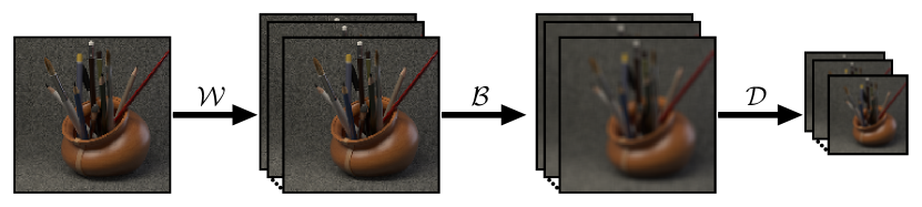
Figure 2: Degradation process

Let us rearrange the 2D angular view of LR SAIs into a 1D set of $s_{k}$ LR observations $Y_{k}\in\mathbb{R}^{s_{y}{\mkern-2.0mu\times\mkern-2.0mu}s_{x}}$, $k\in[1,s_{k}]$. Our goal is to approximate the HR version $X\in\mathbb{R}^{s_{Y}\times s_{X}}$, where $s_{y}\times s_{x}$ and $s_{Y}\times s_{X}$ are the size of LR images and the size of HR image, respectively. In practice, a LR image $Y_{k}$ is considered as a degraded version of the HR image $X$. This degradation can be modelled by the application of three linear operators: warping ($\mathcal{W}_{k}$), blurring ($\mathcal{B}$), and down-sampling ($\mathcal{D}$), as depicted in Fig. 2. The warping operator represents the positioning of the camera. Shifting the camera’s position will result in the corresponding shifts of pixels in the captured image. We define the warping operator as $\mathcal{W}_{k}:\mathbb{R}^{s_{Y}\times s_{X}}\rightarrow\mathbb{R}^{s_{Y}\times s_{X}}$ which transforms a HR image into a new one observed from a different perspective. The blurring operation represents the point spread function (PSF) which describes the response of an imaging system. Depending on the setup of lenses and imaging sensors, PSFs can be very complicated and even spatially variant. However, as shown in the literature Farsiu2004fast ; Sun2020multi , it is sufficient to assume a spatially invariant version of PSF which can be modelled by a linear operator, i.e. $\mathcal{B}:\mathbb{R}^{s_{Y}\times s_{X}}\rightarrow\mathbb{R}^{s_{Y}\times s_{X}}$. The down-sampling operator represents the digital sampling process of an imaging sensor, i.e., $\mathcal{D}:\mathbb{R}^{s_{Y}\times s_{X}}\rightarrow\mathbb{R}^{s_{y}\times s_{x}}$. As a combination of these linear operators, the image foundation process can be described as

$$Y_{k}=\mathcal{D}_{k}\circ\mathcal{B}\circ\mathcal{W}_{k}(X)+\epsilon_{k},\forall k\in[1,s_{k}],$$ (4)

where $\epsilon_{k}$ represents the measurement error or the additive noise which is practically assumed to follow Gaussian distribution or Laplace distribution. For a better presentation, we transform Eq. 4 into vector form,

$$\mathfrak{\textbf{y}}_{k}=DBW_{k}\mathfrak{\textbf{x}}+\boldsymbol{\epsilon}_{k}$$ (5)

where $\mathfrak{\textbf{y}}_{k},\boldsymbol{\epsilon}_{k}\in\mathbb{R}^{s_{x}s_{y}}$ and $\mathfrak{\textbf{x}}\in\mathbb{R}^{s_{X}s_{Y}}$ are the column-vector representations of $Y_{k},\epsilon_{k}$ and $X$. Linear transformation matrices $D$, $B$, and $W_{k}$ respectively replaced the linear operators $\mathcal{D}$, $\mathcal{B}$, and $\mathcal{W}_{k}$. To further simplify the notation, we define $p=s_{X}s_{Y}$, $q=s_{x}s_{y}$, and combine $D,B$ and $W_{k}$ into $A_{k}$, i.e., $A_{k}=DBW_{k}$. It follows that $B,W_{k}\in\mathbb{R}^{p\times p}$, $D\in\mathbb{R}^{q\times p}$, and $A_{k}\in\mathbb{R}^{q\times p}$.

3.2 Bayesian Image Reconstruction Framework

Let us start with the standard Bayesian formulation which poses the SR problem as a maximum a posteriori (MAP) estimation of HR image x given a set of LR samples $\{\mathfrak{\textbf{y}}_{k}\ |\ k=1,..,s_{k}\}$:

$$\tilde{\mathfrak{\textbf{x}}}=\operatorname*{arg\,max}\limits_{\mathfrak{\textbf{x}}}\mathcal{P}(\mathfrak{\textbf{x}}|\mathfrak{\textbf{y}}_{i},...,\mathfrak{\textbf{y}}_{s_{k}}),$$ (6)

where $\mathcal{P}(\mathfrak{\textbf{x}}|\mathfrak{\textbf{y}}_{i},...,\mathfrak{\textbf{y}}_{s_{k}})$ is called posterior and represents the conditional probability density of x given the set of degraded images ($\mathfrak{\textbf{y}}_{k}$). Follow Bayes’ rule, we have

$$\mathcal{P}(\mathfrak{\textbf{x}}|\mathfrak{\textbf{y}}_{1},...,\mathfrak{\textbf{y}}_{s_{k}})=\frac{\mathcal{P}(\mathfrak{\textbf{x}})\prod\limits_{k=1}^{s_{k}}\mathcal{P}(\mathfrak{\textbf{y}}_{k}|\mathfrak{\textbf{x}})}{\prod\limits_{k=1}^{s_{k}}\mathcal{P}(\mathfrak{\textbf{y}}_{k})},$$ (7)

with $\mathcal{P}(\mathfrak{\textbf{y}}_{k}|\mathfrak{\textbf{x}})$ is a likelihood function which encodes the likelihood that the HR image x is due to the LR observation $\mathfrak{\textbf{y}}_{k}$. This function is defined based on the assumption of the noise model of $\boldsymbol{\epsilon}_{k}$. Here, we assume that the noise effecting the observed LR image $\mathfrak{\textbf{y}}_{k}$ is independent. $\mathcal{P}(\mathfrak{\textbf{x}})$ is an image prior describing the properties of the high-resolution image being reconstructed. Since the low-resolution samples are known, $\mathcal{P}(\mathfrak{\textbf{y}}_{k}),k=1,...,s_{k}$, are constants, and the above MAP problem can be transformed into a minimization of negative log-likelihood [0.9] arg max_x P(x—y_1,…,y_s_k) = arg min_x - ln P(x) - ∑_k=1^s_kln P(y_k—x).

The above two logarithmic terms represent the typical setup of an optimization problem consisting of a data fidelity term (i.e., $E(\mathfrak{\textbf{x}}):=-\sum_{k=1}^{s_{k}}ln\mathcal{P}(\mathfrak{\textbf{y}}_{k}|\mathfrak{\textbf{x}})$) and a regularization term (i.e., $R(\mathfrak{\textbf{x}}):=-ln\mathcal{P}(\mathfrak{\textbf{x}})$)

$$\hat{\mathfrak{\textbf{x}}}=\quad\operatorname*{arg\,min}\limits_{\mathfrak{\textbf{x}}}E(\mathfrak{\textbf{x}})+R(\mathfrak{\textbf{x}})$$ (8)

3.3 The Data Fidelity Term

The construction of the data fidelity term depends on the noise models which are practically assumed to follow Gaussian and Laplace distribution Rodriguez2013total . For additive Gaussian noise, $\boldsymbol{\epsilon}_{k}\sim\mathcal{N}(\mu_{k},\sigma_{k}^{2})$ follows a normal distribution with the probability density function given by $\left(1/\sqrt{2\pi\sigma_{k}^{2}}\right)e^{-(\mu_{k}-\boldsymbol{\epsilon}_{k})^{2}/2\sigma_{k}^{2}}$. Assuming a $0$ central distribution (i.e. $\mu_{k}=0$), the likelihood function $\mathcal{P}(\mathfrak{\textbf{y}}_{k}|\mathfrak{\textbf{x}})$ reads

$$\mathcal{P}(\mathfrak{\textbf{y}}_{k}|\mathfrak{\textbf{x}})\propto\texttt{exp}\left(\sum_{k=1}^{s_{k}}\left\lVert A_{k}\mathfrak{\textbf{x}}-\mathfrak{\textbf{y}}_{k}\right\rVert_{2}^{2}\right),$$ (9)

which results in a well-known least square fidelity term. In the case of Laplace noise (i.e., impulse noise), $\boldsymbol{\epsilon}_{k}\sim\mathcal{L}(\mu_{k},b)$ has the probability density function given by $\frac{1}{2b}e^{-\left\lVert\mu_{k}-\boldsymbol{\epsilon}_{k}\right\rVert_{1}/b}$,

$$\mathcal{P}(\mathfrak{\textbf{y}}_{k}|\mathfrak{\textbf{x}})\propto\texttt{exp}\left(\sum_{k=1}^{s_{k}}\left\lVert A_{k}\mathfrak{\textbf{x}}-\mathfrak{\textbf{y}}_{k}\right\rVert_{1}\right).$$ (10)

This results in an $\ell^{1}$ norm data fidelity term, which shows robustness against outliers and superior performance with impulse noise Farsiu2004fast . In order to handle the mixed Gaussian-impulse noise situation, we followed the previous works Jia2016image ; Hakim2020multi to combine $\ell^{1}$ and $\ell^{2}$ norm resulting in a joint $\ell^{1}-\ell^{2}$ data fidelity term,

$$E(\mathfrak{\textbf{x}})=\sum_{l\in\{1,2\}}\lambda_{l}\sum_{k=1}^{s_{k}}\left\lVert A_{k}\mathfrak{\textbf{x}}-\mathfrak{\textbf{y}}_{k}\right\rVert_{l}^{l},$$ (11)

with parameters $\lambda_{1}$ and $\lambda_{2}$ control the contribution of $\ell^{1}$ and $\ell^{2}$ norm respectively.

3.4 Regularization Term

In Bayersian framework, it is generally assumed that x is an Markov random field (MRF) with a strictly positive joint probability density. Therfore, following Hammersly-Clifford theorem, its joint probability density must have the form of a Gibbs distributionGeman1984stochastic :

$$\mathcal{P}(\mathfrak{\textbf{x}})\propto\frac{1}{Z}\texttt{exp}\left(-\frac{1}{T}\sum_{C\in\mathcal{C}}V_{C}(\mathfrak{\textbf{x}})\right),$$ (12)

where $Z$ is a normalizing constant, $T$ stands for temperature and controls the degree of peaking Geman1984stochastic . $V_{C}$ is called potential defined for a local group of pixels or clique $C$. The sum is for a set $\mathcal{C}$ of all possible cliques. The definition of clique set $\mathcal{C}$ and the selection of the potential $V_{C}$ lead to various types of image prior, which share the following form

$$\mathcal{P}(\mathfrak{\textbf{x}})\propto\texttt{exp}\Big{(}\sum\limits_{\mathfrak{\textbf{u}}\in\Omega}\sum\limits_{\mathfrak{\textbf{v}}\in\mathcal{N}(\mathfrak{\textbf{u}})}w(\mathfrak{\textbf{u}},\mathfrak{\textbf{v}})\Phi(\mathfrak{\textbf{x}}_{\mathfrak{\textbf{u}}},\mathfrak{\textbf{x}}_{\mathfrak{\textbf{v}}})\Big{)},$$ (13)

where $\mathfrak{\textbf{u}},\mathfrak{\textbf{v}}\in\Omega$ represents the 2D indices of x. $w:\Omega{\mkern-2.0mu\times\mkern-2.0mu}\Omega\rightarrow\mathbb{R}^{+}$ and $\phi:\mathbb{R}{\mkern-2.0mu\times\mkern-2.0mu}\mathbb{R}\rightarrow\mathbb{R}^{+}$ are respectively weighting function and distance function. The weighting function characterizes the dependency in pixel locations, while the distance function penalizes the difference in pixel intensities. $\mathcal{N}(\mathfrak{\textbf{u}})$ represents a set of indices defined with regarding to the index u. By setting $\Phi$ to the absolute difference, we come to the following weighted regularization term,

$$\mathfrak{\text{R}}(\mathfrak{\textbf{x}})=\sum_{\mathfrak{\textbf{u}}\in\Omega}\sum_{\mathfrak{\textbf{v}}\in\mathcal{N}(\mathfrak{\textbf{u}})}w(\mathfrak{\textbf{u}},\mathfrak{\textbf{v}})|\mathfrak{\textbf{x}}_{\mathfrak{\textbf{u}}}-\mathfrak{\textbf{x}}_{\mathfrak{\textbf{v}}}|,$$ (14)

which can be considered as a generalized version of many total variation based image priors, i.e. TV Rudin1992nonlinear , BTV Farsiu2004fast , NLTV Gilboa2008nonlocal , and BSWTV Sun2021bilateral . In the vector form, Eq. 14 can be rewritten as

$$\mathfrak{\text{R}}(\mathfrak{\textbf{x}})=\sum_{\mathfrak{\textbf{v}}\in\mathcal{N}(\mathfrak{\textbf{u}})}\left\lVert W_{\mathfrak{\textbf{d}}}\odot(S_{\mathfrak{\textbf{d}}}-\text{I})\mathfrak{\textbf{x}}\right\rVert_{1},\quad\mathfrak{\textbf{d}}=\mathfrak{\textbf{u}}-\mathfrak{\textbf{v}},$$ (15)

where $S_{\mathfrak{\textbf{d}}}\in\mathbb{R}^{p\times p}$ denotes the shifting matrix which shift x by d (in 2D coordinate), $\odot$ denotes the Hadamard product. Weighting functions are assembled in weighting matrix $W_{\mathfrak{\textbf{d}}}=\text{diag}(\mathfrak{\textbf{w}}_{\mathfrak{\textbf{d}}})$, with $\mathfrak{\textbf{w}}_{\mathfrak{\textbf{d}}}\in\mathbb{R}^{p}$. The main advantage of this regularization term is the flexibility in defining weighting function to capture unique feature of the SR problem. For example, setting $\mathcal{N}(\mathfrak{\textbf{u}})$ to direct neighborhood and the weighting to a constant gives us TV Rudin1992nonlinear which regularizes the local smoothness between adjacent pixels. Setting weighting to a function of the pixel distance give us BTV Farsiu2004fast , which assumes that the smoothness is spatially dependent. Another weighting scheme based on bilateral spectrum used in  Sun2021bilateral provides a successful regularization for mixed Gaussian-Poisson noise images. Considering the 4D LF data, we proposed a discontinue-aware weighting scheme which assemble three data properties, i.e., spatial distance, edge and occlusion feature,

$$\mathfrak{\textbf{w}}_{\mathfrak{\textbf{d}}}:=w_{d}\mathfrak{\textbf{w}}_{e}\odot\mathfrak{\textbf{w}}_{o},\quad w_{\mathfrak{\textbf{d}}}\in\mathbb{R},\mathfrak{\textbf{w}}_{e},\mathfrak{\textbf{w}}_{o}\in\mathbb{R}^{p},$$ (16)

where the spatial weight $w_{d}:=\texttt{exp}\left(\frac{\left\lVert\mathfrak{\textbf{d}}\right\rVert_{2}^{2}}{\sigma_{s}}\right)$ adjusts the impact of weighting w.r.t. the relative distance d and provide a bilateral filtering effect. The edge weight $\mathfrak{\textbf{w}}_{e}:=\texttt{exp}\left(\frac{\left\lVert\nabla\mathfrak{\textbf{x}}\right\rVert_{2}^{2}}{\sigma_{e}}\right)$ and the occlusion weight $\mathfrak{\textbf{w}}_{o}$ penalize the smoothness at image discontinuing area. We follow the related works Sand2008particle ; Tran2021gvld to define the occlusion weight $\mathfrak{\textbf{w}}_{o}$ as follow,

$$\mathfrak{\textbf{w}}_{o}(\mathfrak{\textbf{z}})=e^{-\frac{b(\mathfrak{\textbf{z}})^{2}}{2\sigma_{o_{1}}^{2}}}e^{-\frac{p(\mathfrak{\textbf{z}})^{2}}{2\sigma_{o_{2}}^{2}}},$$ (17)

where $b(\mathfrak{\textbf{z}})$ and $p(\mathfrak{\textbf{z}})$ are the functions of occlusion boundary and projection error respectively. By an one-side divergence, $b(\mathfrak{\textbf{z}})$ provides weighting to occluding boundary,

$$b(\mathfrak{\textbf{z}})=\left\{\begin{array}[]{ll}\texttt{sum}\{\nabla\boldsymbol{\omega}(\mathfrak{\textbf{z}})\},&\texttt{sum}\{\nabla\boldsymbol{\omega}(\mathfrak{\textbf{z}})\}<0\\ 0,&\text{otherwise}\\ \end{array}\right.,$$ (18)

where $\nabla\boldsymbol{\omega}$ denotes the gradient of a disparity map. The projection error function is computed as the intensity difference between a warped view and the reference view, i.e., $p(\mathfrak{\textbf{z}})=\boldsymbol{L}(\mathfrak{\textbf{z}},\boldsymbol{\theta}_{0})-\boldsymbol{L}(\mathfrak{\textbf{z}}+\boldsymbol{\theta}_{i}\boldsymbol{\omega}(\mathfrak{\textbf{z}}),\boldsymbol{\theta}_{i})$

4 Optimization Approach

Combining the data-fidelity term and regularization term discussed in the previous section, we finalize the minimization problem with the following cost function

$$\begin{split}\mathfrak{\text{J}}(\mathfrak{\textbf{x}})=&\lambda_{1}\sum\limits_{k=1}^{s_{k}}\left\lVert A_{k}\mathfrak{\textbf{x}}-\mathfrak{\textbf{y}}_{k}\right\rVert_{1}+\lambda_{2}\sum\limits_{k=1}^{s_{k}}\left\lVert A_{k}\mathfrak{\textbf{x}}-\mathfrak{\textbf{y}}_{k}\right\rVert_{2}^{2}\\ &\quad+\sum\limits_{d=1}^{s_{d}}\left\lVert W_{d}\odot(S_{d}-\mathfrak{\text{I}})\mathfrak{\textbf{x}}\right\rVert_{1},\end{split}$$ (19)

Although non-smooth, the cost function is convex, and the existence of the global minimized solution is guaranteed. There are many algorithms that can be used to optimize it. One of the traditional approaches to solving this problem is applying a first-order iterative algorithm such as steepest gradient descent. A more recent approach is alternating direction method of multipliers (ADMM) Boyd2011distributed , which breaks a complex optimization problem into smaller sub-problems, each can be solved in a simpler manner. Although ADMM requires more computation for each iterative step as compared to gradient descent, we notice that the overall computation of ADMM is much less considering the similar minimization threshold. We start with rewriting the objective function into a more compact form,

$$\mathfrak{\text{J}}(\mathfrak{\textbf{x}})=\left\lVert A\mathfrak{\textbf{x}}-\mathfrak{\textbf{b}}\right\rVert_{2}^{2}+\left\lVert F\mathfrak{\textbf{x}}-\mathfrak{\textbf{b}}^{\prime}\right\rVert_{1},$$ (20)

the matrices $F$, $A$ and columns vectors b, $\mathfrak{\textbf{b}}^{\prime}$ are defined as in Eq. 20. Notice that $\lambda_{1}$ and $\lambda_{2}$ are absorbed into the matrices and column vectors for simplifying the notation. The sizes of $A$, $F$, b and $\mathfrak{\textbf{b}}^{\prime}$ are respectively $qs_{k}\times p$, $(qs_{k}+ps_{d})\times p$, $qs_{k}\times 1$ and $(qs_{k}+ps_{d})\times 1$. All transformation matrices ($A_{k}$ and $S_{d}$) and weighting matrices ($W_{d}$) are assembled into $A$ and $F$. Low-resolution images $b_{k}$ are stacked into b. $O_{ps_{d}}$ is zero vector with the size of $ps_{d}\times 1$. [0.88] &A := λ_2 [A1A2… Ask], b:= λ_2[y1y2… ysk]
F := [λ1λ2A S ], b’ := [λ1λ2bOpsd], S := [W1⊙(S1-I) W2⊙(S2-I)… Wsd⊙(Ssd-I) ]

Taking the compact representation, we rewrite the optimization problem in Eq. 19 into the form of ADMM problem,

$$\begin{split}&\operatorname*{minimize}_{\mathfrak{\textbf{x}},\mathfrak{\textbf{z}}}\quad\left\lVert A\mathfrak{\textbf{x}}-\mathfrak{\textbf{b}}\right\rVert_{2}^{2}+\left\lVert\mathfrak{\textbf{z}}\right\rVert_{1}\\ &\operatorname*{subject\,to}\quad F\mathfrak{\textbf{x}}-\mathfrak{\textbf{z}}=\mathfrak{\textbf{b}}^{\prime},\end{split}$$ (21)

with the augmented Lagragian reads, [0.95] L_ϑ(x, z, w)& :=∥Ax- b∥_2^2 + ∥z∥_1
+ w^⊺(Fx- z-b’) + ϑ2 ∥Fx- z-b’∥_2^2

The ADMM problem, Eq. 21, is then broken into the following sub-problems for the two unknowns x and z.

$$\mathfrak{\textbf{x}}^{(k+1)}= \operatorname*{arg\,min}_{\mathfrak{\textbf{x}}}\mathcal{L}_{\vartheta}(\mathfrak{\textbf{x}},\mathfrak{\textbf{z}}^{(k)},\mathfrak{\textbf{w}}^{(k)})$$

$$= \operatorname*{arg\,min}_{\mathfrak{\textbf{x}}}\left\lVert A\mathfrak{\textbf{x}}-\mathfrak{\textbf{b}}\right\rVert_{2}^{2}+\frac{\vartheta}{2}\left\lVert F\mathfrak{\textbf{x}}-\mathfrak{\textbf{z}}^{(k)}-\mathfrak{\textbf{b}}^{\prime}+\frac{\mathfrak{\textbf{w}}^{(k)}}{\vartheta}\right\rVert_{2}^{2}$$

$$\mathfrak{\textbf{z}}^{(k+1)}= \operatorname*{arg\,min}_{\mathfrak{\textbf{x}}}\mathcal{L}_{\vartheta}(\mathfrak{\textbf{x}}^{(k+1)},\mathfrak{\textbf{z}},\mathfrak{\textbf{w}}^{(k)})$$

$$= \operatorname*{arg\,min}_{\mathfrak{\textbf{z}}}\left\lVert\mathfrak{\textbf{z}}\right\rVert_{1}+\frac{\vartheta}{2}\left\lVert\mathfrak{\textbf{z}}-\left(F\mathfrak{\textbf{x}}^{(k+1)}-\mathfrak{\textbf{b}}^{\prime}+\frac{\mathfrak{\textbf{w}}^{(k)}}{\vartheta}\right)\right\rVert_{2}^{2}$$

$$\mathfrak{\textbf{w}}^{(k+1)}= \mathfrak{\textbf{w}}^{(k)}+\vartheta\big{(}F\mathfrak{\textbf{x}}^{(k+1)}-\mathfrak{\textbf{z}}^{(k+1)}-\mathfrak{\textbf{b}}^{\prime}\big{)}$$

The sub-problem of z, in Eq. 22b, is actually a proximal operator of $\ell^{1}$ function,

$$\mathfrak{\textbf{z}}^{(k+1)}=\mathfrak{\textbf{prox}}_{\vartheta^{-1}\left\lVert\cdot\right\rVert_{1}}\left(F\mathfrak{\textbf{x}}^{(k+1)}-\mathfrak{\textbf{b}}^{\prime}+\frac{\mathfrak{\textbf{w}}^{(k)}}{\vartheta}\right),$$

which has the following closed form solution

$$\begin{split}\mathfrak{\textbf{z}}^{(k+1)}=&\left[\left\lvert F\mathfrak{\textbf{x}}^{(k+1)}-\mathfrak{\textbf{b}}^{\prime}+\frac{\mathfrak{\textbf{w}}^{(k)}}{\vartheta}\right\rvert-\frac{1}{\vartheta}\right]_{+}\\ &\quad\odot\mathfrak{\textbf{sgn}}\left(F\mathfrak{\textbf{x}}^{(k+1)}-\mathfrak{\textbf{b}}^{\prime}+\frac{\mathfrak{\textbf{w}}^{(k)}}{\vartheta}\right)\end{split}$$ (23)

The sub-problem of x (Eq. 22a) has the form of a least square approximation problem,

$$\begin{split}\tilde{\mathfrak{\textbf{x}}}=\operatorname*{arg\,min}\limits_{\mathfrak{\textbf{x}}}\left\lVert G\mathfrak{\textbf{x}}-\mathfrak{\textbf{c}}\right\rVert_{2}^{2}\end{split},$$ (24)

with $G=\begin{bmatrix}A\\ \sqrt{\vartheta/2}F\end{bmatrix}$ , and $\mathfrak{\textbf{c}}=\begin{bmatrix}\mathfrak{\textbf{b}}\\ \sqrt{\vartheta/2}\left(\mathfrak{\textbf{z}}^{(k)}+\mathfrak{\textbf{b}}^{\prime}-\mathfrak{\textbf{w}}^{(k)}/\vartheta\right)\end{bmatrix}$ . Equation 24 can be effectively solved with a conjugate gradient approach on normal equation Boyd2004convex .

4.1 Treatment of Linear Operators

All computations are eventually broken down to matrix multiplication for which the largest computational efforts are on $A_{k},S_{d},\quad k\in[1,s_{k}],d\in[1,s_{d}]$, and their adjoint versions $A_{k}^{\intercal},S_{d}^{\intercal}$. These matrixes are very large and sparse. For example, given a pair of low-resolution and high-resolution: $s_{x}\times s_{y}:=128\times 128$ and $s_{X}\times s_{Y}=512\times 512$ (i.e., $4\times$ super-resolution). Assuming $s_{k}=16$ and $s_{d}=8$, the size of $A$ is $2^{18}\times 2^{18}$ and the size of $S$ is $2^{21}\times 2^{18}$. Direct computation of these matrixes is infeasible. Therefore, we decided to implement these matrices in the form of linear functions of 2D variables instead of sparse matrix and vectorized inputs.

Figure 3: Implementation of downsampling operator

For downsampling operator $\mathcal{D}$, a simple resampling scheme is employed as depicted in Fig. 3. For each block of $\contour[1]{black}{$\zeta$}_{x}\times\contour[1]{black}{$\zeta$}_{y}$ pixels, one pixel at the top-left location is picked and put into the low-resolution grid. The adjoint operator $\mathcal{D}^{*}$ is therefore simply putting back the corresponding pixel to this location. The bluring operator $\mathcal{B}$ is modelled by a simple Gaussian kernel with a standard deviation of $\sigma=\frac{1}{4}\sqrt{\contour[1]{black}{$\zeta$}^{2}-1}$ and a size of $3\sigma$ as suggested in Unger2010convex . The warping operator $\mathcal{W}_{k}$ and its adjoint operator $\mathcal{W}_{k}^{*}$ are implemented as forward-warping and backward-warping functions. These functions are associated with a set of disparity maps at each of the perspectives employed for super-resolution. Assumes that a set of $s_{k}$ low-resolution sub-aperture images each with its perspective index is in $P=\{\boldsymbol{\theta}_{1},\boldsymbol{\theta}_{2},...,\boldsymbol{\theta}_{s_{k}}\}$ are inputs to estimate an super-resoltion image at $\boldsymbol{\theta}_{0}\in P$. For each perspective $\boldsymbol{\theta}_{k}$, we need to find the disparity map $\boldsymbol{\omega}_{k}$. The forward warping function $\mathcal{W}_{k}$ will warp the SAI from perspective $\boldsymbol{\theta}_{0}$ to $\boldsymbol{\theta}_{k}$ using $\boldsymbol{\omega}_{k}$, i.e., $\contour[1]{black}{$\widehat{L}$}(\mathfrak{\textbf{z}},\boldsymbol{\theta}_{k})=\boldsymbol{L}(\mathfrak{\textbf{z}}+\boldsymbol{\theta}_{k}\boldsymbol{\omega}_{k},\boldsymbol{\theta}_{k})$, while the backward warping function $\mathcal{W}_{k}^{*}$ will warp the input SAI from perspective $\boldsymbol{\theta}_{k}$ to $\boldsymbol{\theta}_{0}$ using $\boldsymbol{\omega}_{0}$, i.e., $\contour[1]{black}{$\widehat{L}$}(\mathfrak{\textbf{z}},\boldsymbol{\theta}_{0})=\boldsymbol{L}(\mathfrak{\textbf{z}}+\boldsymbol{\theta}_{0}\boldsymbol{\omega}_{0},\boldsymbol{\theta}_{0})$.

The transformation matrix $S$ can be implemented in the form of weighted directional gradient ($\nabla^{U,V}$) computed for a direction set $U=\{\mathfrak{\textbf{d}}_{i}|\mathfrak{\textbf{d}}_{i}\in\mathbb{N}^{2},i=1,..,s_{d}\}$ and a weight set $V=\{V_{i}|V_{i}\in\mathbb{R}^{s_{X}{\mkern-2.0mu\times\mkern-2.0mu}s_{Y}},i=1,..,s_{d}\}$. Let $I$ be the SAI at perspective $\boldsymbol{\theta}_{0}$, $I(\mathfrak{\textbf{z}})=\boldsymbol{L}(\mathfrak{\textbf{z}},\boldsymbol{\theta}_{0})$, we computed $\nabla^{U,V}I$ as follow,

$$\boldsymbol{G}=\nabla^{U,V}I=\left(\frac{\partial}{\partial\mathfrak{\textbf{d}}_{1}},\frac{\partial}{\partial\mathfrak{\textbf{d}}_{2}},..,\frac{\partial}{\partial\mathfrak{\textbf{d}}_{s_{d}}}\right)I,$$ (25)

with the weighted directional derivative $\partial/\partial\mathfrak{\textbf{d}}_{i}$ approximated by finite differences,

$$\boldsymbol{G}_{d_{i}}(\mathfrak{\textbf{z}})=\frac{\partial}{\partial\mathfrak{\textbf{d}}_{i}}I(\mathfrak{\textbf{z}})=V_{i}(\mathfrak{\textbf{z}})\left(I(\mathfrak{\textbf{z}})-I(\mathfrak{\textbf{z}}+\mathfrak{\textbf{d}}_{i})\right).$$ (26)

The adjoint matrix $S^{\intercal}$ is then computed in the form of weighted directional divergence,

$$\texttt{div}^{U,V}\boldsymbol{G}=\nabla^{U,V}\cdot\boldsymbol{G}=\sum_{i=1}^{s_{d}}\frac{\partial\boldsymbol{G}_{\mathfrak{\textbf{d}}_{i}}}{\partial\mathfrak{\textbf{d}}_{i}}.$$ (27)

5 GPU-Accelerated Architecture

This section presents the accelerated architecture for 4D LFSR. Acceleration is achieved by parallel computation on graphics processing units. Due to the multi-platform compatibility, we select OpenCL over CUDA for the implementation of the proposed approach. To solve the cost function optimization problem of Eq. 19, we follow the iterative solving process discussed in Sec. 4. As will be discussed later in the experimental results (Sec. 7.1), the ADMM solver provides better performance in optimizing the cost function as compared to the gradient descent approach.

Input: $\vartheta,\mathfrak{\textbf{x}}_{0},N$

Output: x

1 $\mathfrak{\textbf{x}}^{(0)}:=\mathfrak{\textbf{x}}_{0}$

2 $\mathfrak{\textbf{w}}^{(0)}:=0$

3 for $n$ in $1,2,..N$ do

4       $\mathfrak{\textbf{a}}:=A\mathfrak{\textbf{x}}^{(n-1)}-\mathfrak{\textbf{b}}$

5       $\mathfrak{\textbf{u}}:=F\mathfrak{\textbf{x}}^{(n-1)}-\mathfrak{\textbf{b}}^{\prime}+\mathfrak{\textbf{w}}^{(n-1)}$

       $\mathfrak{\textbf{z}}^{(n)}:=\mathfrak{\textbf{prox}}_{\rho^{-1}\left\lVert\cdot\right\rVert_{1}}(\mathfrak{\textbf{u}})$

        $\triangleright$ Solving Eq. 22b

       $\mathfrak{\textbf{w}}^{(n)}:=\mathfrak{\textbf{u}}-\mathfrak{\textbf{z}}^{(n)}$

        $\triangleright$ Computing Eq. 22c

6       $\mathfrak{\textbf{f}}:=2\mathfrak{\textbf{w}}^{(n)}-\mathfrak{\textbf{w}}^{(n-1)}$

7       $\mathfrak{\textbf{v}}:=A^{\intercal}\mathfrak{\textbf{a}}+\frac{\vartheta}{2}F^{\intercal}\mathfrak{\textbf{f}}$

       $\mathfrak{\textbf{x}}^{(n)}:=\texttt{xstep}(\mathfrak{\textbf{v}},\mathfrak{\textbf{x}}^{(n-1)})$

        $\triangleright$ Solving Eq. 22a

8      

9 end for

10return $\mathfrak{\textbf{x}}^{(n)}$

Algorithm 1 Minimization of the cost function in Eq. 19 with ADMM iterative solver.

For a better handling of the computation flow, we did the following modifications to ADMM iteration in Eq. 22. First, the order of sub-problems is rearranged such that x-step comes after z-step and w-step. This way allows us to make use of the computation of $F\mathfrak{\textbf{x}}$ for all sub-problems. Secondly, the parameter $\vartheta$ is absorbed into w (i.e., w instead of $\mathfrak{\textbf{w}}/\vartheta$) to save unnecessary scalar multiplications. $\vartheta$ only takes part in the computation of proximal operator ($z$-step) and solving of the least square problem ($x$-step). Fig. 4 illustrates the modified computations of ADMM solver which is also listed in Algorithm 1.

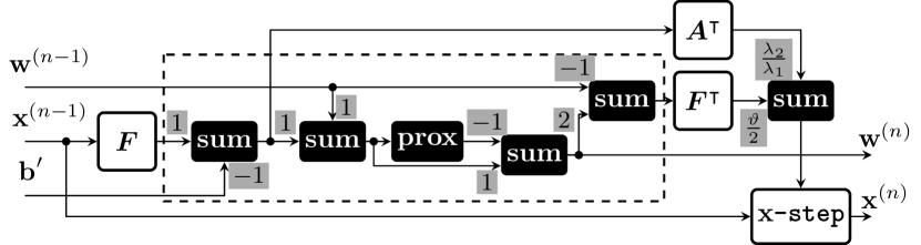
Figure 4: Computation flow of one ADMM iteration.

The ADMM solver takes in three arguments, the parameter $\vartheta$, an initial guess ($\mathfrak{\textbf{x}}_{0}$) and the number of iterations ($N$), as in Algorithm 1. Before the iteration, we initialized x with $\mathfrak{\textbf{x}}_{0}$, a bi-cubic up-sampling of the low-resolution image, and w with zeros, line $1,2$. Each iteration starts with the computation of $A\mathfrak{\textbf{x}}$ and $F\mathfrak{\textbf{x}}$ which are associated to $\ell^{2}$ and $\ell^{1}$ terms of the objective function, Eq. 20. While $A\mathfrak{\textbf{x}}$ is subtracted by b, line $4$, $F\mathfrak{\textbf{x}}$ is subtracted by $\mathfrak{\textbf{b}}^{\prime}$ and summed with w, line $5$. Since $F$ is a stack of $A$ and $S$ and $\mathfrak{\textbf{b}}^{\prime}$ includes b, Eq. 20, we avoid the re-computation of $A\mathfrak{\textbf{x}}-\mathfrak{\textbf{b}}$ by extracting it from $F\mathfrak{\textbf{x}}-\mathfrak{\textbf{b}}^{\prime}$ as depicted in Fig. 4. The sum and subtract operations in line $5$ are realized by two-arguments sum kernels (i.e., sum in Fig. 4). The gray box attached to each input to the sum kernel denotes the scalar scaling of the input. On line $6$, we conduct a z-step by computing the proximal operator of u. This proximal operator is realized by an OpenCL kernel prox, as in Fig. 4, followed by a sum kernel which realizes w-step, line $7$ Algorithm 1.

After the computation of z and w, the next step is preparing the residual input for the conjugate gradient descent solver in x-step, $\mathfrak{\textbf{v}}=G^{\intercal}(G\mathfrak{\textbf{x}}-\mathfrak{\textbf{c}})$. From Eq. 24, we have [0.9] v=& [Aϑ/2F]^T [Ax-bϑ/2(Fx- z(n)-b’+w(n))]
= A^⊺(Ax-b) + ϑ/2 F^⊺(Fx-z^(n)-b’+w^(n))
= A^⊺a+ ϑ2 F^Tf

With the computation of f, Algorithm 1 line $8$, as $\mathfrak{\textbf{f}}=2\mathfrak{\textbf{w}}^{(n)}-\mathfrak{\textbf{w}}^{(n-1)}=\mathfrak{\textbf{u}}-\mathfrak{\textbf{z}}-\mathfrak{\textbf{w}}^{(n-1)}+\mathfrak{\textbf{w}}^{(n)}=F\mathfrak{\textbf{x}}^{(n-1)}-\mathfrak{\textbf{z}}-\mathfrak{\textbf{b}}^{\prime}+\mathfrak{\textbf{w}}^{(n)}$. The computations of f and v are realized by two sum kernels directly before and after $F^{T}$ as in Fig. 4. Notice that we made a scaling of $A^{T}\mathfrak{\textbf{a}}$ by $\frac{\lambda_{2}}{\lambda_{1}}$ since a is extracted from $F\mathfrak{\textbf{x}}-\mathfrak{\textbf{b}}^{\prime}$ which has a different scalar scaling of matrix $A$ and column vector b. Another note from the implementation of Fig. 4 is that the group of OpenCL kernels marked by dashed rectangle would be combined into a single kernel, since these kernels share element-wise operators.

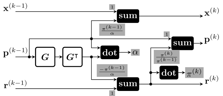
Figure 5: Computation flow of xstep.

As discussed in the previous section, conjugate gradient descent on normal equation is employed to solve $\ell^{2}$ optimization problem of x-step. Fig. 5 depicts the computation flow of x-step, while its pseudo code is listed in Algorithm 2. There are two inputs, i.e. v, $\mathfrak{\textbf{x}}^{(n-1)}$, and two scalar parameters, i.e., $\tau$, $K$. The computed HR image from the previous ADMM iteration $\mathfrak{\textbf{x}}^{(n-1)}$ is used as the initial guess for the conjugate gradient descent solver, while the residual v is used to initialize $\mathfrak{\textbf{r}}^{(0)}$, $\mathfrak{\textbf{p}}^{0}$ and compute the initial error $\pi^{(0)}$. The two parameters $\tau$ and $K$ specify the error threshold and the maximum number of conjugate gradient iterations, respectively. The stop condition is that either the residual r is sufficiently small or the maximum number of iterations is reached, Algorithm 2 line $4$,$5$. All computations in Algorithm 2 can be effectively broken down into GPU kernel implementation. Beside the forward and backward transform ($G,G^{\intercal}$), there are two kernels sum and dot, as in Fig. 5, which represents element-wise sum and dot product respectively.

From the Eq. 20 and Eq. 24, we can derive the computation of $G^{T}G$ in the form of $A$ and $S$ as

$$\small\begin{split}G^{T}G=A^{T}A+\frac{\vartheta}{2}F^{\intercal}F=\left(1+\frac{\vartheta}{2}\frac{\alpha_{1}^{2}}{\alpha_{2}}\right)A^{T}A+\frac{\vartheta}{2}S^{T}S,\end{split}$$ (28)

with the kernel realization of $A$,$S$ and its adjoint version $A^{\intercal}$, $S^{\intercal}$ shown in Fig. 6. The figure illustrates the change in the size of the column vector after each kernel execution. Regarding Fig. 6, fwarp, bwarp, blur, up, and down denote the forward warp, backward warp, blur, up-sampling and down-sampling kernel respectively. wdg kernel realizes the weighted directional gradient (i.e., $\nabla^{U,V}$), while the weighted directional divergence (i.e., $\texttt{div}^{U,V}$) is implemented by wdd kernel.

Input: $\mathfrak{\textbf{v}},\mathfrak{\textbf{x}}^{(n-1)},\tau,K$

Output: x

1 $\mathfrak{\textbf{x}}^{(0)}:=\mathfrak{\textbf{x}}^{(n-1)}$

2 $\mathfrak{\textbf{p}}^{(0)}:=\mathfrak{\textbf{r}}^{(0)}:=\mathfrak{\textbf{v}}$

$\pi^{(0)}:=<\mathfrak{\textbf{r}}^{(0)},\mathfrak{\textbf{r}}^{(0)}>$

  $\triangleright$ dot product

3 for $k$ in $1,2,..K$ do

4       if $\pi^{(k-1)}<\tau$ then

5             $\mathfrak{\textbf{v}}:=G^{{\intercal}}G\mathfrak{\textbf{p}}^{(k-1)}$

6             $\alpha:=<\mathfrak{\textbf{v}},\mathfrak{\textbf{p}}^{(k-1)}>$

7             $\mathfrak{\textbf{r}}^{(k)}:=\mathfrak{\textbf{r}}^{(k-1)}-\frac{\pi^{(k-1)}}{\alpha}\mathfrak{\textbf{v}}^{(k-1)}$

8             $\pi^{(k)}:=<\mathfrak{\textbf{r}}^{(k)},\mathfrak{\textbf{r}}^{(k)}>$

9             $\mathfrak{\textbf{p}}^{(k)}:=\mathfrak{\textbf{p}}^{(k-1)}+\frac{\pi^{(k)}}{\pi^{(k-1)}}\mathfrak{\textbf{r}}^{(k-1)}$

10             $\mathfrak{\textbf{x}}^{(k)}:=\mathfrak{\textbf{x}}^{(k-1)}+\frac{\pi^{(k-1)}}{\alpha}\mathfrak{\textbf{p}}^{(k-1)}$

11            

12       end if

13      

14 end for

15return $\mathfrak{\textbf{x}}^{(k)}$

Algorithm 2 Solving x-step

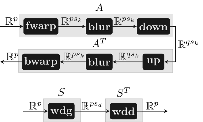
Figure 6: Kernel realization of $A,A^{\intercal},S,S^{\intercal}$

6 Limitation and Discussion

Although the strategy to realize the degradation process with linear functions has the advantage of saving computational resources and simplifying the GPU implementation, it presents a drawback in dealing with a more challenging blurring process, i.e., space-variant PSFs. In this work, we assume that the PSF is space-invariant and can be approximated by a single Gaussian blur kernel. However, depending on the optical setup, the blurring process may involve a set of space-variant PSFs. This means that each blur kernel may only be applied to a group of pixels, and different regions of an image would require different blur kernels. In such a case, sparse matrix realization of blurring operator would be a reasonable option to avoid the complication of maintaining and applying region-specific blur kernel.

Beside Gaussian and Impulse noise, there is another challenging noise originating from the discrete nature of the electric charge, namely photon noise or shot noise Hasinoff2014photon . Different from additive Gaussian noise, which is pixel independent, the photon noise is pixel dependent and follows the Poisson distribution. Taking the notation from Sec. 3.1, the degradation model considering Poisson noise and additive Gaussian noise reads

$$\mathfrak{\textbf{y}}_{k}=\mathfrak{\textbf{z}}_{k}+\boldsymbol{\epsilon},$$ (29)

where $\mathfrak{\textbf{z}}_{k}\sim\mathcal{P}(A_{k}\mathfrak{\textbf{x}})$ and $\boldsymbol{\epsilon}\sim\mathcal{N}(0,\sigma^{2})$ represent the Poisson distribution and a zero-mean Gaussian distribution, respectively. Following the work in Sun2020multi , we can rewrite our data fidelity term as [0.9] E(x) = ∑_k=1^s_k∥A_kx-y_k∥_W_k^2 + ¡log(A_kx+ σ^2),1¿, where $log(\cdot)$ is computed element-wise and diagonal weight matrix $W_{i}$ is computed as

$$W_{k}=diag\left(\frac{1}{[A_{k}\mathfrak{\textbf{x}}]_{i}+[\sigma]_{i}^{2}}\right),$$ (30)

with $[\mathfrak{\textbf{x}}]_{i}$ denotes the $i^{th}$ element of column vector x. As discussed in Sun2020multi , although $\ell 1$/$\ell 2$ data terms can also be applied to input data with Poisson noise, their reconstruction quality is about 1dB worse as compared to applying Eq. 29. Due to the $log$ function, the above data term will lead to a non-convex optimization problem in which a global minimum is not guaranteed. For solving this new problem, a new decomposing strategy with ADMM needs to be developed. This task, together with the acceleration of the new solving process, is listed in our plan for future work.

7 Experimental Results

This section discusses the results of our experiments, in which the robustness of the proposed SR model is validated through numerous testing scenarios. Comparisons to the state-of-the-art approaches under severe mixed noise conditions and previous GPU acceleration approaches are presented. In addition, the performance of the accelerated computational framework is also analyzed and discussed.

7.1 Evaluation of LFSR Computational Framework

Light-field scenes from 4D synthetic dataset Honauer2016dataset are employed to evaluate the robustness of the SR model and analyze the converge of iterative solvers. This dataset is selected since it includes plenty of scenery and provides accurate disparity maps. We follow the degradation model discussed in Sec. 3.1 to prepare the input data with two test scaling factors, i.e., ${\mkern-2.0mu\times\mkern-2.0mu}2$, ${\mkern-2.0mu\times\mkern-2.0mu}4$. The observation noises are parameterized by $\sigma$ and $\nu$, which respectively denotes the standard deviation of Gaussian noise (i.e., $\mathcal{N}(\mu,\sigma)$) and the percentage of impulse noise (i.e., salt and pepper). In order to match the practical use cases in which the high-resolution disparity maps are not available, the provided disparity maps are down-scaled by the same factor as of the test case (i.e., ${\mkern-2.0mu\times\mkern-2.0mu}2$, ${\mkern-2.0mu\times\mkern-2.0mu}4$) and then are interpolated back to the original size and used in the warping functions. For handling color input data, we follows the strategy proposed in Tran2018gpu to solve the cost function for $Y$ color channel while applying bi-cubic interpolation for $Cb$ and $Cr$ channel.

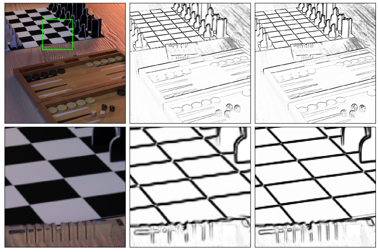
(a)                     (b)                     (c)

Figure 7: Regularization weights calculation for LF scene ‘boardgames’; top row: full size image and weights; bottom row: zoom-in of region marked by green rectangle; (a) Ground-truth image; (b) weights at the $1^{st}$ iteration; (c) weights after the $10^{th}$ iteration.

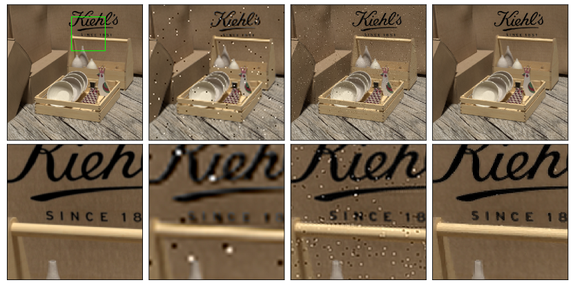
(a)                 (b)                 (c)                 (d)

Figure 8: $\times 4$ super-resolution of LF scene ‘dishes’ ($\sigma=1$, $\nu=1\%$); top row: full size image; bottom row: zoom-in of region marked by green rectangle; (a) Ground-truth image; (b) bi-cubic up-sampling (21.72 dB); (c) 1st iteration (24.96 dB) (d) 5th iteration (29.53 dB)

The regularization weights computed for the scene ‘boardgames’ are shown Fig. 7. It is expected that a strong weighting is applied to the region where high-frequency information occupied (i.e., texture edges, occlusions). As discussed in Sec. 3.4, the regularization weight is a combination of spatial weight ($w_{d}$), edge weight ($\mathfrak{\textbf{w}}_{e}$), and occlusion weight ($\mathfrak{\textbf{w}}_{o}$). To strengthen the regularizing effect, the weights are recomputed for each ADMM iteration using the current computed super-resolution image x. When the optimization starts, x is initialized to a bi-cubic up-sampling of the low-resolution image. This explains the blur edges of regularization weights at iteration 1, as shown in Fig. 7 (b). However, it could be observed after each ADMM iteration that the qualities of x and regularization weight are gradually improved. As shown in Fig. 7 (c), the regularization weight after 10 ADMM iterations capture well the high-resolution structure of the reconstructed scene.

Fig. 8 visualizes the SR result for the ${\mkern-2.0mu\times\mkern-2.0mu}4$ test case of LF scene ‘dishes’. We employed 17 LR sub-aperture images as inputs to calculate the cost function in Eq. 19 which is then solved by ADMM iterative solver. The SAIs are picked up from $5{\mkern-2.0mu\times\mkern-2.0mu}5$ angular views in a star-like structure. As compared to the bi-cubic up-sampling image used as an initial solution (Fig. 8 (b)), the reconstructed HR image after the first ADMM iteration (Fig. 8 (c)) demonstrates an obvious improvement in visibility. Although the noise effect from the combination of multiple SAIs is still visible, it is possible to observe the texture content (i.e., small characters in the middle of the zoom-in region). After 5 ADMM iterations, the noise effect is removed, resulting in a significant enhancement in visual quality with 4.6dB and 7.8dB improvement as compared to the 1st iteration’s solution and the initial solution, respectively.

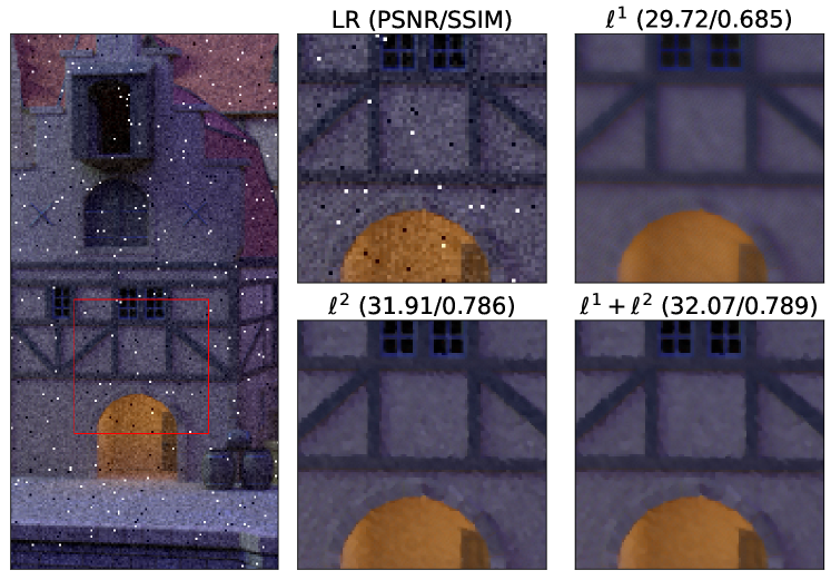
Figure 9: $\times 2$ super-resolution of LF scene ‘medieval2’ ($\sigma=10,\nu=1\%$); left : a cropped noisy LR input; right: four zoom-in of the marked region from an LR input and three different configurations of data fidelity term.

(a)                   (b)                   (c)                   (d)                   (e)                   (f)                   (g)

Figure 10: Super-resolution $\times 4$ results of LF scene ‘vinyl’ under different number of inputs. top full size HR image; bottom zoom-in of marked region; (a) Ground-truth image; (b) bi-cubic upsampling (24.04dB); (c) 3 SAIs (27.55dB); (d) 5 SAIs (29.33dB); (e) 9 SAIs (30.54dB); (f) 25 SAIs (31.65dB); (g) 49 SAIs (32.09dB).

To evaluate the contribution of $\ell^{1}$ and $\ell^{2}$ data terms in reconstructing HR perspective image under mix-noise condition, we prepare a test case in which LR Light-field is severely damaged by noise effects, see Fig. 9. While keeping the regularization part unchanged, we tuned data fidelity parameters ($\lambda_{1}$, $\lambda_{2}$) to find a solution with the highest PSNR score for each model (i.e., $\ell^{1}$, $\ell^{2}$, $\ell^{1}+\ell^{2}$). We observed that using only $\ell^{2}$ data fidelity tends to oversmooth the solution due to the effect of the $\ell^{2}$ norm. Although $\ell^{1}$ data fidelity well preserves the sharp edge structure, it also carries the effect of the noisy pixels into the solution. The proposed mix-noise data term combines the impacts of both $\ell^{2}$ norm and $\ell^{1}$ norm and provides a better reconstruction quality.

The number of input LR images play an important role in the quality of reconstructed HR image. Although demanding higher computation resources, we observed that more input SAIs tend to provide higher reconstruction qualities. Fig. 10 reports the $\times 4$ super-resolution results of LF scene ‘vinyl’ where different numbers of LR sub-aperture images are used. As can be seen from the figure, giving more input images to the computational problem (Eq. 19) results in the better visual quality of HR solutions, which is also evident from the reported PSNR scores. Specifically, an improvement of 3.5dB as compared to bi-cubic up-sampling can be achieved with three input images. When increasing the number of LR images to 5, 9, 25, and 49, we observed the incremental gains of 1.8dB, 1.2 dB, 1.1 dB and 0.44 dB, respectively.

In order to compare the convergence of the iterative solvers, we employ the matrix transform functions (i.e.,$A$,$S$) and their adjoint versions (i.e., $A^{\intercal}$, $S^{\intercal}$) as computation units (CU). As derived in Sec. 4, these transforms are the most dominant computation tasks and exist in every iterative step. Each CU is either a combination of $A$ and $S$ as for computing the cost function J or $A^{\intercal}$ and $S^{\intercal}$ as for computing the gradient $\nabla\mathfrak{\text{J}}$. In this experiment, we built a cost function for $\times 2$ SR problem of LF scene ‘vinyl’ and applied four different configurations of the iterative solvers to optimize it. The first two are gradient descent solver (GD) without and with line search denoted as gd and gd-ls respectively. The last two are ADMM solvers in which we configure the maximum number of conjugate gradient steps to 5 (admm-5) and 10 (admm-10). Fig. 11 presents the plot of the loss function against the accumulated CU. Providing a good step size, GD without line search can make a rapid reduction in the cost function for the first few iterations. However, due to fixed step size, the GD cannot optimize the loss function further after 80 CUs. In contrast, gd-ls seems slow at the beginning due to the search for an appropriate step size but is able to surpass gd at around 100 CUs and approach the global minimum after around 300 CUs. Avoiding the costly line-search tasks, both configurations of the ADMM solver demonstrate a superior convergence rate as compared to GD. We also observed that setting the maximum number of conjugate descent steps to 5 does shorten the computation effort for the first few iterations. However, at later iterations when the early stop condition is satisfied, i.e., Algorithm 2 line 5, both settings result in a similar performance.

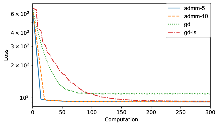
Figure 11: Optimization results of different solvers.

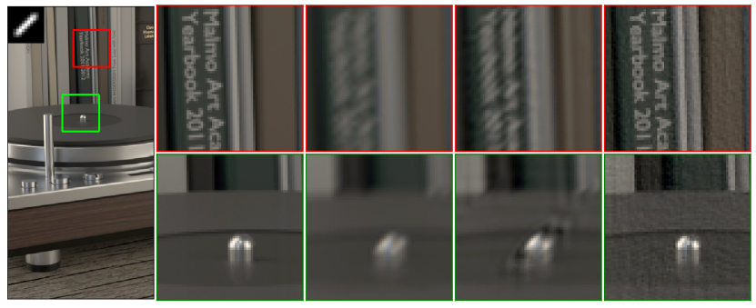
(a)             (b)             (c)             (d)             (e)

Figure 12: ${\mkern-2.0mu\times\mkern-2.0mu}2$ super-resolution result of LF scene ‘vinyl’ degraded by motion blur. (a) a cropped of ground truth with two marked region and motion blur kernel shown at top left corner; (b) zoom-in of ground truth image; (c) bi-cubic initial image (26.86dB); (d) after $1^{st}$ ADMM iteration (30.27dB); (e) after $10^{th}$ ADMM iteration (35.43dB).

The proposed computation framework can also be applied to a more challenging image condition such as motion blur. In such a case, the motion blur can be modelled by a convolutional kernel as a realization of the linear operator $\mathcal{B}$ (see Fig. 2). Fig. 12 shows our ${\mkern-2.0mu\times\mkern-2.0mu}2$ SR result for low-resolution LF input degraded by a 45 degree motion blur. The blur kernel is shown on the top left corner of Fig. 12(a) and two zoom-in regions of the bi-cubic upsampling of degraded low-resolution SAI are shown in Fig. 12(c). Taking 25 SAIs as inputs to our reconstruction algorithm, we can achieve more than a 3 dB improvement in PSNR score after one ADMM iteration. The high-resolution LF image is well reconstructed after $10^{th}$ ADMM iterations with clear texture information and motion trace.

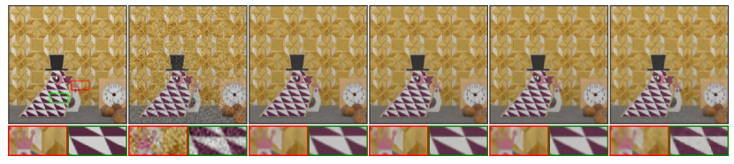
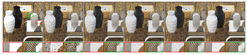
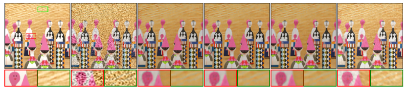
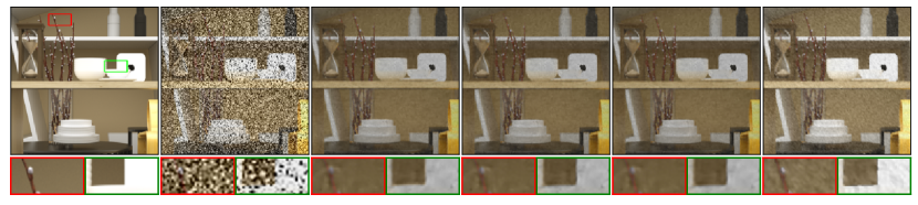
Ground Truth         Input SAI             De-resLF             De-3DVSR              DRLF                  Ours

Figure 13: Visual comparisons of LFSR approaches under various mixed noise settings. From top to bottom (‘scene’ - $\sigma$/$\nu$): ‘Rooster-clock’ - 20/0; ‘Coffee-beans-vases’ - 20/5; ‘Smiling-crowd’ - 50/0; ‘Dishes’ - 50/20.

7.2 Comparison to LFSR Approaches

In this section, we evaluate the performance of the proposed method under severe mixed noise conditions and compare it to state-of-the-art approaches (i.e., resLF Zhang2019residual , DRLF Guo2021deep , and 3DVSR Tran20223dvsr ). These approaches currently provide state-of-the-art performance in reconstructing high-resolution LF images. To the best of our knowledge, only DRLF Guo2021deep supports LFSR with noisy input. For the evaluation, we randomly select five scenes from the Inria LF dataset Shi2019framework . For each scene we generate low resolution LF (${\mkern-2.0mu\times\mkern-2.0mu}2$) and insert noises with four configurations, ($\sigma\texttt{=}20,\nu\texttt{=}0\%$), ($\sigma\texttt{=}20,\nu\texttt{=}5\%$), ($\sigma\texttt{=}50$, $\nu\texttt{=}0\%$), ($\sigma\texttt{=}50,\nu\texttt{=}20\%$). These Gaussian noise settings are selected due to the pre-trained weights published by DRLF. DRLF needs different trainings for dealing with different noise conditions, and there are only three pre-trained weights published for three Gaussian noise configurations $\sigma\texttt{=}10$, $\sigma\texttt{=}20$, and $\sigma\texttt{=}50$. In addition, DRLF does not directly process noisy LR inputs. It provides separate networks for de-nosing and super-resolution. Therefore, we applied first their de-noising network to noisy LR inputs and then applied their SR network to the de-noised LR outputs. In this way, we are able to evaluate the performance of the other two state-of-the-art LFSR approaches (i.e., resLF Zhang2019residual , 3DVSR Tran20223dvsr ) using the de-noised LR output from DRLF.

Table 1: Quantitative comparison of LFSR approaches under various mixed noise settings.

Noise	Scenes	BIC	resLF	De+resLF	3DVSR	De+3DVSR	DRLF	Ours
($\sigma/\nu$)		(psnr/ssim)	(psnr/ssim)	(psnr/ssim)	(psnr/ssim)	(psnr/ssim)	(psnr/ssim)	(psnr/ssim)
20/0	Dishes	22.63/0.378	21.20/0.316	28.80/0.886	19.32/0.252	28.74/0.891	28.71/0.888	30.47/0.846
	Rooster-clock	22.81/0.375	21.24/0.304	30.73/0.864	19.36/0.241	31.15/0.879	30.84/0.881	31.48/0.798
	Coffee-beans-vases	21.55/0.507	20.41/0.453	25.24/0.801	18.86/0.389	25.51/0.812	25.62/0.818	26.31/0.801
	Smiling-crowd	21.81/0.493	20.56/0.428	25.93/0.836	18.84/0.359	26.11/0.853	25.97/0.851	29.27/0.832
	Electro-devices	22.67/0.322	21.17/0.260	28.41/0.824	19.28/0.201	28.67/0.836	28.26/0.823	30.74/0.793
2-92.0	mean	22.29/0.415	20.91/0.352	27.82/0.842	19.13/0.288	28.04/0.854	27.88/0.852	29.66/0.814
20/5	Dishes	18.89/0.283	17.51/0.234	26.15/0.671	15.31/0.177	25.31/0.629	26.18/0.663	30.36/0.843
	Rooster-clock	19.19/0.267	17.69/0.212	27.91/0.710	15.42/0.158	27.18/0.680	27.80/0.720	31.39/0.794
	Coffee-beans-vases	18.25/0.394	16.99/0.342	23.56/0.646	14.96/0.274	23.13/0.625	23.81/0.652	26.22/0.797
	Smiling-crowd	18.14/0.383	16.86/0.329	23.97/0.693	14.53/0.249	23.17/0.658	23.86/0.695	29.12/0.829
	Electro-devices	18.93/0.231	17.51/0.184	26.00/0.631	15.30/0.135	25.29/0.595	25.76/0.621	30.65/0.789
2-92.0	mean	18.68/0.312	17.31/0.260	25.52/0.670	15.10/0.199	24.82/0.638	25.48/0.670	29.55/0.810
50/0	Dishes	16.11/0.162	14.56/0.129	20.81/0.819	11.81/0.086	20.51/0.818	20.62/0.821	27.74/0.715
	Rooster-clock	15.90/0.133	14.28/0.101	21.62/0.787	11.43/0.065	21.36/0.789	21.28/0.793	28.55/0.669
	Coffee-beans-vases	15.92/0.246	14.44/0.196	19.85/0.693	11.83/0.138	19.69/0.694	19.71/0.709	24.26/0.672
	Smiling-crowd	16.28/0.247	14.80/0.203	19.02/0.686	12.13/0.146	18.88/0.695	18.91/0.692	26.40/0.717
	Electro-devices	15.99/0.120	14.41/0.093	21.10/0.743	11.60/0.062	20.92/0.745	20.81/0.732	28.20/0.662
2-92.0	mean	16.04/0.182	14.50/0.145	20.48/0.746	11.76/0.100	20.27/0.748	20.27/0.749	27.03/0.687
50/20	Dishes	13.00/0.094	11.78/0.075	18.87/0.743	9.50/0.047	18.66/0.736	18.85/0.745	26.89/0.704
	Rooster-clock	13.23/0.080	11.91/0.061	19.76/0.721	9.48/0.038	19.56/0.714	19.40/0.721	27.80/0.675
	Coffee-beans-vases	12.78/0.145	11.61/0.115	17.82/0.622	9.45/0.077	17.69/0.618	17.60/0.635	23.78/0.674
	Smiling-crowd	12.66/0.148	11.52/0.121	16.44/0.621	9.44/0.083	16.33/0.622	16.39/0.625	25.54/0.721
	Electro-devices	13.05/0.068	11.78/0.053	19.40/0.690	9.45/0.033	19.25/0.684	19.09/0.677	27.44/0.656
2-92.0	mean	12.94/0.107	11.72/0.085	18.46/0.680	9.46/0.056	18.30/0.675	18.26/0.681	26.29/0.686

The experimental results are reported in Table 1 and visualized in Fig. 13. For the two approaches, resLF and 3DVSR, which do not support noisy LF input, we generate de-noised LF with DRLF and use it as an input to resLF and 3DVSR. These results are denoted as De+resLF and De+3DVSR respectively. For all noise settings, our approach provides the best reconstruction quality in terms of PSNR. For mixed noise settings, the proposed method achieves an averagely highest SSIM score as compared to the other approaches. These high scores pay tribute to the robustness of the proposed model in which de-noising and super-resolution are jointly resolved. Without de-nosing resLF and 3DVSR completely fails to reconstruct a good quality HR image. In practice, they up-scale not only the texture but also the existing noise. Their scores are, therefore, even worse as compared to bi-cubic upsampling approach in which noise are blurred out. From Fig. 13, it is evident that the reconstructed HR image from the other approaches is over-smoothed while our approach preserves well the texture content and high-frequency information, e.g., and object edges in Dishes scene, background pattern in Smiling-crowd scene. Since DRLF supports only Gaussian noise, it fails to recognize impulse noise in the LR input. The impulse noise is either ignored, i.e., when Gaussian noise level is low, or mistreated, i.e., in a severe Gaussian noise setting. Consequently, the reconstructed HR images are presented with noisy traces, i.e., Coffee-beans-vases scene or losing texture detail, i.e., the flower bud in Dishes scene.

7.3 Comparison to GPU-Accelerated Approach

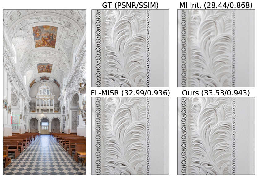
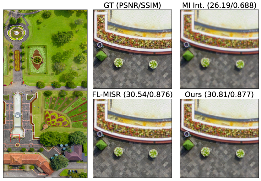
Figure 14: HR reconstruction results of DIV8K dataset Gu2019div8k . top ${\mkern-2.0mu\times\mkern-2.0mu}2$ results of image 0002; bottom ${\mkern-2.0mu\times\mkern-2.0mu}3$ results of image 0084.

As discussed in Sec. 3.1, the proposed framework shares a similar setup as a multi-frame super-resolution problem and indeed can be applied as well for this kind of problem. To evaluate the performance of our accelerated framework, we conducted an experiment on the natural image dataset DIV8K Gu2019div8k and compared to recent related work on the field (FL-MISR Sun2021fl ). We follow the experimental setup described in Sun2021fl to prepare the low-resolution images and perform the HR image reconstruction with our accelerated solver. Particularly, we pick up seven images from DIV8K dataset and generate, for each of them, four LR images for ${\mkern-2.0mu\times\mkern-2.0mu}2$ SR and nine LR images for ${\mkern-2.0mu\times\mkern-2.0mu}3$ SR. The shifting of ${\mkern-2.0mu\times\mkern-2.0mu}2$ and ${\mkern-2.0mu\times\mkern-2.0mu}3$ image sets are respectively $\frac{1}{2}$px and $\frac{1}{3}$px. The Gaussian noise is configured with $\sigma=1$. Since FL-MISR use $\ell^{1}$ data fidelity and BTV regularization in their model, we turn off our $\ell^{2}$ term and configure nonlocal weighting (i.e. $W_{\mathfrak{\textbf{d}}}$) to match BTV condition. The accelerated ADMM iterative solver is then executed to minimize the cost function in Eq. 19. For a fair comparison, we stop our iterative solver as soon as the quality of the reconstructed image is comparable to FL-MISR and measure the execution time. Quantitative evaluation results are listed in Table 2, while visual comparison is given in Fig. 14 From the table, it is obvious that our GPU accelerated solver outperforms FL-MISR in processing speed for all test cases while providing a better reconstruction quality. As compared to FL-MISR, our GPU-based solver achieves an average speed-up of 2.46${\mkern-2.0mu\times\mkern-2.0mu}$ and 1.57${\mkern-2.0mu\times\mkern-2.0mu}$ for up-scaling ${\mkern-2.0mu\times\mkern-2.0mu}2$ and up-scaling ${\mkern-2.0mu\times\mkern-2.0mu}3$ respectively. This performance boost tributes to the effectiveness of ADMM solver and the realization strategy of transformation matrices ($A_{k},S_{\mathfrak{\textbf{d}}}$). In contrast to FL-MISR, which chooses to implement $A_{k},S_{\mathfrak{\textbf{d}}}$ with sparse matrices, our approach takes advantage of linear functions (i.e., $\mathcal{W},\mathcal{B},\mathcal{D}$) to optimize GPU memory and computation resource. Therefore, our GPU-based solver can fit well within a single GTX 1080Ti GPU, while FL-MISR needs four of them to solve the same problem.

Table 2: Evaluation of parallel computing approach for MISR problem on 8-bit natural images in DIV8K dataset. MI Int.: Multi-image interpolation (56 cores Intel Xeon Gold 5120), FL-MISR Sun2021fl (4 GTX 1080Ti), ours (1 GTX 1080Ti).

Image Index		0001	0002	0007	0027	0055	0066	0084
Resolution of GT		5376$\times$5760	5568$\times$5760	1920$\times$2880	2112$\times$2880	5760$\times$5760	1920$\times$2880	5760$\times$3840
Upscaling 2$\times$
MI Int.	PSNR/SSIM	30.49/0.9215	28.44/0.8677	33.68/0.8810	28.37/0.8988	33.80/0.9018	35.21/0.9296	29.11/0.8277
	Runtime ($s$)	0.51	0.52	0.11	0.20	0.53	0.11	0.36
FL-MISR	PSNR/SSIM	37.11/0.9620	32.99/0.9360	35.09/0.9111	33.21/0.9417	38.03/0.9564	37.12/0.9452	34.13/0.9410
	Runtime ($s$)	1.50	1.29	0.69	0.71	1.3	0.66	1.21
Ours	PSNR/SSIM	37.24/0.9713	33.53/0.9430	35.42/0.9220	33.73/0.9497	38.13/0.9616	37.51/0.9539	34.60/0.9454
	Runtime ($s$)	0.92	1.14	0.15	0.24	0.72	0.18	0.83
Upscaling 3$\times$
MI Int.	PSNR/SSIM	26.74/0.8460	25.65/0.7749	32.03/0.8395	25.15/0.8212	30.79/0.8153	32.65/0.8968	26.19/0.6883
	Runtime ($s$)	1.00	0.99	0.11	0.13	0.55	0.11	0.38
FL-MISR	PSNR/SSIM	33.24/0.9446	29.43/0.8941	33.99/0.8941	30.17/0.9139	35.90/0.9379	36.06/0.9398	30.54/0.8764
	Runtime ($s$)	1.78	1.73	0.32	0.38	1.93	0.35	1.65
Ours	PSNR/SSIM	33.39/0.9517	30.04/0.9017	34.50/0.8984	30.57/0.9293	36.22/0.9402	36.35/0.9447	30.81/0.8774
	Runtime ($s$)	1.13	1.17	0.23	0.25	1.22	0.23	0.84

7.4 Performance Analysis of OpenCL-based Solvers

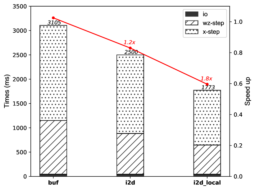
Figure 15: Cumulative execution time and speed-up of three realization strategies.

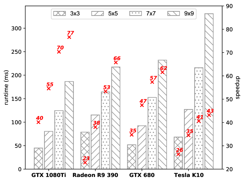
Figure 16: Execution of GPU-based solver under different number of inputs on various OpenCL platforms.

For analyzing the performance improvement of the proposed GPU accelerated approach, we perform an evaluation of three realization strategies of ADMM iterative solvers. Fig. 15 reports the cumulative execution time of the three GPU implementations. The initial GPU implementation (i.e., buf) is considered as a baseline, in which a 1D buffer object is used for holding variable and input data in GPU global memory. In the second implementation, denoted as $i2d$, 1D buffer objects are replaced by Image2D objects. This allows us to make use of the texture cache provided in GPU architecture for speeding up the access to image-like data. The third implementation, denoted as $i2d\_local$ takes advantage of local memory for buffering and sharing data within a work-group. Since local memory is close to the computing unit, this provides a high-speed data pool for kernel tasks which frequently require access to multiple neighbor pixels (i.e. blurring, warping). For this experiment, we use $5{\mkern-2.0mu\times\mkern-2.0mu}5$ angular views as input for ${\mkern-2.0mu\times\mkern-2.0mu}4$ SR to a spatial resolution of $512{\mkern-2.0mu\times\mkern-2.0mu}512$. The number of ADMM iterations and CG iterations is set to 10 and 5, respectively. The execution time of the ADMM solver can be divided into three parts. The $io$ part covers the time for transferring input data from CPU memory into GPU global memory and reading back the reconstructed HR image from GPU to GPU memory. The $wz-step$ part represents the computation time of updating w and z in an ADMM iteration, while $x-step$ part measures the time to solve for x by applying conjugate gradient descent technique, see Fig. 4. As could be seen from Fig. 15, the IO time only accounts for a small amount of overall execution time, while most of the time is spent on $x-step$ and $wz-step$. As compared to the $buf$ version, the texture cache provided by Image2D object $i2d$ does shorten the computation time of ADMM solver by a factor of 1.2$\times$. The local memory sharing technique further speeds up the computation time by a factor of 1.8$\times$.

The advantage of using the OpenCL framework is that the accelerated solver can be executed on various platforms. Fig. 16 shows the execution time of $i2d\_local$ on various GPU platforms. In this test, we vary the number of input LR images: 9, 25, 49, and 81, which are denoted as $3\times 3$,$5\times 5$,$7\times 7$, and $9\times 9$, respectively. The regularization window size is configured to $5{\mkern-2.0mu\times\mkern-2.0mu}5$, and the number of conjugate gradient steps is set to 5. For each case, we measure the execution time of a single ADMM iteration and compare it to the CPU implementation, executed on i7-5820K 3.30GHz. In general, we observed a higher speed up as compared to CPU execution when more input images are provided. The speedup ranges from 23$\times$ to 40$\times$ in the case of $3\times 3$ inputs and from 43$\times$ to 77$\times$ in the case of $9\times 9$ inputs.

8 Conclusion

This paper presents a GPU-accelerated computational framework for reconstructing high-resolution SAI from 4D LF data under mixed Gaussian-Impulse noise conditions. The proposed SR model derived from a statistical perspective takes advantage of a joint $\ell^{1}-\ell^{2}$ data fidelity term for dealing with mixed noise conditions and weighted non-local total variation for enforcing LF image prior. Our approach combines the de-noising effect and SR reconstruction into a single optimization problem which, as shown in the experimental results, allows us to surpass the current state-of-the-art approaches in which de-noise and SR problems are resolved separately. The non-smooth convex optimization problem resulting from the proposed SR model is effectively solved by ADMM algorithm. By transforming the minimization of $\ell^{1}-\ell^{2}-\ell^{1}$ mixture cost function into least square approximation and proximal operator problems, ADMM overcomes the main problem of gradient descent technique in finding a suitable step-size. We showed that GPU acceleration is well-suited to speeding up the iteratively solving process. To verify the robustness of the proposed SR model and evaluate the performance of the accelerated optimizer, an extensive experiment is conducted on 4D synthetic LF dataset and high-resolution natural image dataset. The experimental results show that the proposed approach outperforms the previous work in accelerating the super-resolution task and optimizing GPU resources. While providing a better reconstruction quality, our accelerated framework provides an average speed up of 2.46${\mkern-2.0mu\times\mkern-2.0mu}$ and $1.57{\mkern-2.0mu\times\mkern-2.0mu}$ for ${\mkern-2.0mu\times\mkern-2.0mu}2$ and ${\mkern-2.0mu\times\mkern-2.0mu}3$ SR tasks, respectively. The accelerated solver achieves a speedup of 77${\mkern-2.0mu\times\mkern-2.0mu}$ as compared to CPU implementation.

The proposed approach encourages further research directions on both algorithmic and computing architecture levels. In the first direction, we would extend the SR model to handle a more challenging noise setting, i.e., photon noise, which follows the Poisson distribution. Solving such a problem would require a new ADMM decomposing strategy for the non-convex non-smooth optimization problem. In the second direction, the iterative solving process could be realized on a field-programmable gate array (FPGA) platform on which we could achieve much higher processing speed and much lower energy consumption as compared to GPU. For this task, the main challenges lie in the realization of the warping function and the access of 4D-LF data on hardware.

References

- (1) E. H. Adelson, J. Y. A. Wang, Single lens stereo with a plenoptic camera, IEEE Trans. Pattern Anal. Mach. Intell. (2) (1992) 99–106.
- (2) M. Levoy, P. Hanrahan, Light field rendering, in: ACM Proc. 23rd Annu. Conf. Comput. Graph. Interact. Tech., 1996, pp. 31–42.
- (3) J. C. Silva, M. Saadi, L. Wuttisittikulkij, D. R. Militani, R. L. Rosa, D. Z. Rodríguez, S. Al Otaibi, Light-field imaging reconstruction using deep learning enabling intelligent autonomous transportation system, IEEE Transactions on Intelligent Transportation Systems (2021).
- (4) R. S. Overbeck, D. Erickson, D. Evangelakos, M. Pharr, P. Debevec, A system for acquiring, processing, and rendering panoramic light field stills for virtual reality, ACM Transactions on Graphics (TOG) 37 (6) (2018) 1–15.
- (5) L. Ni, Z. Li, H. Li, X. Liu, 360-degree large-scale multiprojection light-field 3d display system, Applied optics 57 (8) (2018) 1817–1823.
- (6) J. Unger, A. Wenger, T. Hawkins, A. Gardner, P. Debevec, Capturing and rendering with incident light fields, Tech. rep., Inst. Creative Tech., Univ. Southern California (2003).
- (7) B. Wilburn, N. Joshi, V. Vaish, E.-V. Talvala, E. Antunez, A. Barth, A. Adams, M. Horowitz, M. Levoy, High performance imaging using large camera arrays, in: ACM Trans. Graph., Vol. 24, ACM, 2005, pp. 765–776.
- (8) Z. Cheng, Z. Xiong, C. Chen, D. Liu, Light field super-resolution : A benchmark, in: CVPR Work., 2019.
- (9) Y. Yuan, Z. Cao, L. Su, Light-field image superresolution using a combined deep cnn based on epi, IEEE Signal Process. Lett. 25 (9) (2018) 1359–1363.
- (10) S. Zhang, Y. Lin, H. Sheng, Residual networks for light field image super-resolution, IEEE Conf. Comput. Vis. Pattern Recognit. (2019) 11046–11055.
- (11) T.-H. Tran, J. Berberich, S. Simon, 3dvsr: 3d epi volume-based approach for angular and spatial light field image super-resolution, Signal Processing 192 (2022) 108373.
- (12) T. E. Bishop, P. Favaro, The light field camera: Extended depth of field, aliasing, and superresolution, IEEE Transactions on Pattern Analysis and Machine Intelligence 34 (5) (2012) 972–986.
- (13) M. Rossi, P. Frossard, Geometry-consistent light field super-resolution via graph-based regularization, IEEE Transactions on Image Processing 27 (9) (2018) 4207–4218.
- (14) M. Alain, A. Smolic, Light field super-resolution via lfbm5d sparse coding, in: 2018 25th IEEE International Conference on Image Processing (ICIP), 2018, pp. 2501–2505.
- (15) J. Kim, J. K. Lee, K. M. Lee, Accurate image super-resolution using very deep convolutional networks, in: 2016 IEEE Conf. Comput. Vis. Pattern Recognit., IEEE, 2016, pp. 1646–1654.
- (16) B. Lim, S. Son, H. Kim, S. Nah, K. M. Lee, Enhanced deep residual networks for single image super-resolution, in: IEEE Conf. Comput. Vis. Pattern Recognit. Work., 2017.
- (17) K. Sun, T.-H. Tran, J. Guhathakurta, S. Simon, Fl-misr: fast large-scale multi-image super-resolution for computed tomography based on multi-gpu acceleration, Journal of Real-Time Image Processing (2021) 1–14.
- (18) K. Honauer, O. Johannsen, D. Kondermann, B. Goldluecke, A dataset and evaluation methodology for depth estimation on 4d light fields, in: Asian Conf. Comput. Vis., Springer, 2016, pp. 19–34.
- (19) J. Shi, X. Jiang, C. Guillemot, A framework for learning depth from a flexible subset of dense and sparse light field views, IEEE Transactions on Image Processing (2019) 5867–5880.
- (20) S. Gu, A. Lugmayr, M. Danelljan, M. Fritsche, J. Lamour, R. Timofte, Div8k: Diverse 8k resolution image dataset, in: Int. Conf. on Comp. Vis. Work., 2019, pp. 3512–3516.
- (21) T. H. Tran, G. Mammadov, K. Sun, S. Simon, Gpu-accelerated light-field image super-resolution, in: Proc. - 2018 Int. Conf. Adv. Comput. Appl. ACOMP 2018, IEEE, 2018, pp. 7–13.
- (22) T.-H. Tran, Z. Wang, S. Simon, Variational disparity estimation framework for plenoptic images, in: IEEE Int. Conf. Multimed. Expo, 2017, pp. 1189–1194.
- (23) H. W. F. Yeung, J. Hou, X. Chen, J. Chen, Z. Chen, Y. Y. Chung, Light field spatial super-resolution using deep efficient spatial-angular separable convolution, IEEE Transactions on Image Processing 28 (5) (2018) 2319–2330.
- (24) H. Fan, D. Liu, Z. Xiong, F. Wu, Two-stage convolutional neural network for light field super-resolution, in: Int. Conf. Image Process., IEEE, 2017, pp. 1167–1171.
- (25) M. Guo, J. Hou, J. Jin, J. Chen, L.-P. Chau, Deep spatial-angular regularization for light field imaging, denoising, and super-resolution, IEEE Transactions on Pattern Analysis & Machine Intelligence (01) (2021) 1–1.
- (26) A. Ivan, I. Kyu Park, Others, Light field depth estimation on off-the-shelf mobile gpu, in: IEEE Conf. Comput. Vis. Pattern Recognit. Work., 2018, pp. 634–643.
- (27) T.-H. Tran, G. Mammadov, S. Simon, Gvld: A fast and accurate gpu-based variational light-field disparity estimation approach, IEEE Transactions on Circuits and Systems for Video Technology 31 (7) (2021) 2562–2574.
- (28) I. K. Park, K. M. Lee, Others, Robust light field depth estimation using occlusion-noise aware data costs, Trans. Pattern Anal. Mach. Intell. 40 (10) (2018) 2484–2497.
- (29) S. Farsiu, M. D. Robinson, M. Elad, P. Milanfar, Fast and robust multiframe super resolution, IEEE Transactions on Image Processing 13 (10) (2004) 1327–1344.
- (30) K. Sun, T.-H. Tran, R. Krawtschenko, S. Simon, Multi-frame super-resolution reconstruction based on mixed poisson–gaussian noise, Signal Processing: Image Communication 82 (2020) 115736.
- (31) P. Rodríguez, Total variation regularization algorithms for images corrupted with different noise models: A review, J. Electr. Comput. Eng. 2013 (1) (2013).
- (32) T. Jia, Y. Shi, Y. Zhu, L. Wang, An image restoration model combining mixed l1/l2 fidelity terms, J. Vis. Commun. Image Represent. 38 (2016) 461–473.
- (33) M. Hakim, A. Ghazdali, A. Laghrib, A multi-frame super-resolution based on new variational data fidelity term, Applied Mathematical Modelling 87 (2020) 446–467.
- (34) S. Geman, D. Geman, Stochastic Relaxation, Gibbs Distributions, and the Bayesian Restoration of Images, IEEE Transactions on Pattern Analysis and Machine Intelligence PAMI-6 (6) (1984) 721–741.
- (35) L. I. Rudin, S. Osher, E. Fatemi, Nonlinear total variation based noise removal algorithms, Physica D: nonlinear phenomena 60 (1-4) (1992) 259–268.
- (36) G. Gilboa, S. Osher, Nonlocal operators with applications to image processing, Multiscale Modeling and Simulation 7 (3) (2008) 1005–1028. doi:10.1137/070698592.
- (37) K. Sun, S. Simon, Bilateral spectrum weighted total variation for noisy-image super-resolution and image denoising, IEEE Trans. Signal Process. 69 (2021) 6329–6341.
- (38) P. Sand, S. Teller, Particle video: Long-range motion estimation using point trajectories, Int. J. Comput. Vis. 80 (1) (2008) 72.
- (39) S. Boyd, N. Parikh, E. Chu, Distributed optimization and statistical learning via the alternating direction method of multipliers, Now Publishers Inc, 2011.
- (40) S. Boyd, L. Vandenberghe, Convex Optimization, Cambridge University Press, 2004.
- (41) M. Unger, T. Pock, M. Werlberger, H. Bischof, A convex approach for variational super-resolution, in: Joint pattern recognition symposium, Springer, 2010, pp. 313–322.
- (42) S. W. Hasinoff, Photon, Poisson Noise, Springer US, Boston, MA, 2014, pp. 608–610.