Positional Label for Self-Supervised Vision Transformer

Abstract

Positional encoding is important for vision transformer (ViT) to capture the spatial structure of the input image. General effectiveness has been proven in ViT. In our work we propose to train ViT to recognize the positional label of patches of the input image, this apparently simple task actually yields a meaningful self-supervisory task. Based on previous work on ViT positional encoding, we propose two positional labels dedicated to 2D images including absolute position and relative position. Our positional labels can be easily plugged into various current ViT variants. It can work in two ways: (a) As an auxiliary training target for vanilla ViT (e.g., ViT-B Dosovitskiy et al. (2020) and Swin-B Liu et al. (2021)) for better performance. (b) Combine the self-supervised ViT (e.g., MAE He et al. (2021)) to provide a more powerful self-supervised signal for semantic feature learning. Experiments demonstrate that with the proposed self-supervised methods, ViT-B and Swin-B gain improvements of 1.20% (top-1 Acc) and 0.74% (top-1 Acc) on ImageNet, respectively, and 6.15% and 1.14% improvement on Mini-ImageNet.

1 Introduction

Vision transformers (ViT) Dosovitskiy et al. (2020); Zhao et al. (2020) have recently emerged as an alternative to convolutional neural networks (CNNs) in computer vision. The design of ViT is inspired by the transformer of natural language processing (NLP), split an image into patches and provide the sequence of linear embeddings of these patches as an input to a Transformer Touvron et al. (2021). Image patches are treated the same way as tokens (words) in NLP. The core of transformer is self-attention Vaswani et al. (2017), which is able to model long-range dependencies in the data. However, self-attention is fully symmetric, it cannot capture the ordering of input tokens, which is undesirable for modeling structured data. Therefore, incorporating positional encoding is especially important for ViT.

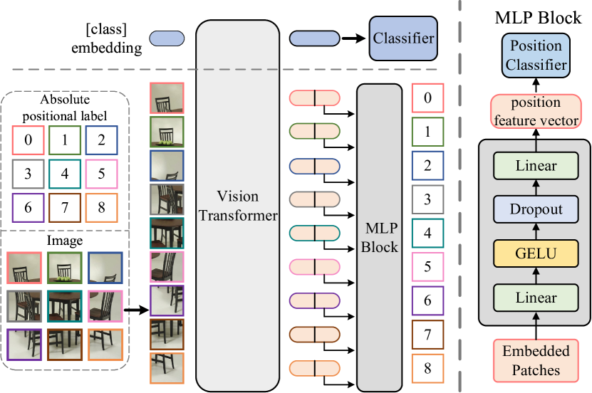
Figure 1: Our absolute positional label combined with ViT-B. We split an image into fixed-size patches, each corresponding to an absolute position, and feed the sequence of image patches to a standard ViT encoder. The full set of encoded patches output (intercept half) by the ViT is processed by a lightweight MLP block that outputs the positional feature vector corresponding to each image patch, which is finally fed into a positional classifier for training, the same as for vanilla classification. After training, the MLP block is discarded.

There are mainly two classes of methods to add positional information for ViT. One is absolute and the other is relative. Absolute positional encoding Gehring et al. (2017); Li et al. (2018): each absolute position of the input token sequence from 1 to maximum sequence length has a separate encoding vector. The encoding vector is then combined with the input tokens, usually element-wise add, to incorporate positional information into the ViT’s input tokens. On the other hand, relative positional encoding Dai et al. (2019); Shaw et al. (2018) calculates the relative position between tokens based on the absolute position of each input token, and establishes a look-up table. Each relative position corresponds to a learnable parameter of the table to learn the pairwise relations of tokens. The parameters in the table interact with the self-attention weights. Relative positional encoding has been verified to be effective in ViT Wu et al. (2021). Different from the previous explicit incorporation of positional information, we use the positional information as a supervision signal for ViT self-supervised training, making each encoded patch implicitly contains its positional information, as shown in Figure 1.

In this paper, we seek to expand the applicability of positional information to serve as a supervised signal for self-supervised training of ViT. Based on the positional information, we propose a new ViT self-supervised loss function, namely position loss, which allows each token to implicitly contain its positional information. Specifically, we split an image into fixed-size patches and feed the sequence of image patches to a standard ViT. The full set of encoded patches output by the ViT is processed by a lightweight MLP block that outputs the positional label corresponding to each image patch. Based on previous research on ViT positional encoding, we propose two positional labels for ViT: absolute and relative positional labels. Section 3 illustrates how to apply these two positional labels to ViT and their differences.

Our position loss can work in two ways: (a) Combined with vanilla ViT (e.g., ViT-B Dosovitskiy et al. (2020) and swin transformer Liu et al. (2021)), as an auxiliary training task for the model. The ViT is trained under the joint supervision of the softmax loss and position loss, with a hyperparameter to balance the two supervision signals. We find that with joint supervision, the classification performance of ViT is significantly improved. (b) Combined with self-supervised ViT, e.g., MAE He et al. (2021). MAE masks random patches from the input image and reconstructs the missing patches in the pixel space. Our position loss combined with MAE, allowing the model to not only reconstructs the pixels of the missing patches, but also outputs the positional information of the patches, providing a more powerful self-supervised signal for semantic feature learning. Our contributions can be summarized as:

• We propose two positional labels, absolute and relative positional labels, for ViT self-supervised learning. We also introduce efficient implementations of these two positional labels that can be easily plugged into self-attention layers.

• Our proposed positional label can be used as an alternative for positional encoding, which implicitly adds positional information to each image patch through ViT self-supervised training.

• The proposed positional labels can be combined with vanilla ViT and self-supervised ViT. Experiments show that, without adjusting any hyperparameters and settings, ViT-B and Swin-B obtained improvements of 1.20% (top-1 Acc) and 0.74% (top-1 Acc) on ImageNet, respectively. More improvements on the small dataset, ViT-B and Swin-B obtained improvements of 6.15% (top-1 Acc) and 1.14% (top-1 Acc) on Mini-ImageNet, respectively.

2 Related Work

2.1 Self-Supervised ViT

In pioneering works Chen et al. (2020); He et al. (2021), training self-supervised Transformers for vision problems in general follows the masked auto-encoding paradigm in NLP Devlin et al. (2018); Wang et al. (2019). iGPT Chen et al. (2020) masks and reconstructs pixels. MAE He et al. (2021) masks a high proportion of the input image patches and reconstruct the missing patches. DINO Caron et al. (2021) studies the importance of momentum encoder, multi-crop training Caron et al. (2020), and the use of small patches with ViTs, to design a simple self-supervised approach that can be interpreted as a form of knowledge distillation with no labels. Chen et al. (2021) focuses on training Transformers in the contrastive/Siamese paradigm, in which the loss is not defined for reconstructing the inputs. DILEMMA Sameni et al. (2022) proposes a pseudo-task to train a ViT to detect which input token has been combined with an incorrect positional embedding to boost both shape and texture discriminability in models trained via self-supervised learning. In this work, we propose a novel self-supervised learning signal for ViT, named positional labels.

2.2 Positional Encoding

(a) Absolute Positional Encoding. Since transformer contains no recurrence and no convolution, in order for the model to make use of the order of the sequence, we need to inject some information about the position of the tokens. The original self-attention considers the absolute position, and add the absolute positional encodings to the input token embedding by element-wise addition Vaswani et al. (2017). There are several choices of absolute positional encodings, such as Sinusoidal position Vaswani et al. (2017) fixed encoding using sine and cosine functions sampling at different frequencies and Gehring et al. (2017) the learnable encoding via training parameters.

(b) Relative Positional Encoding. Relative positional encoding is proposed firstly by Shaw et al. (2018), extending the self-attention mechanism to efficiently consider representations of the relative positions, where relative positional encodings are added into the self-attention weight calculation. Dai et al. (2019) proposed a novel positional encoding scheme with the prior of the sinusoid matrix and more learnable parameters, which not only enables capturing longer-term dependency, but also resolves the context fragmentation problem. Wu et al. (2021) proposes new relative positional encoding methods dedicated to 2D images, called image RPE (iRPE). iRPE considers directional relative distance modeling as well as the interactions between queries and relative positional embeddings in self-attention mechanism. Ramachandran et al. (2019) proposed 2D relative positional encoding that computes and concatenates separate encodings of each dimension. Srinivas et al. (2021) proposes to incorporate the positional information in the convolutional feature map into ViT by concatenating the convolutional feature map with a set of feature maps produced via the self-attentive mechanism.

Unlike the previous explicit combination of positional information, we use the positional information as a supervised signal for ViT self-supervised training, such that each encoded patch implicitly contains its positional information. Section 4.2 discusses the relationship between our positional label and conventional positional encoding and demonstrates that they can be used jointly.

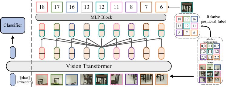
Figure 2: Our relative positional label combined with ViT-B. For the brevity of the image, here we take the relative positional label of the central image patch of the input image as an example, and the rest of the image patches are calculated in the same way. We combine the center encoded patch with other encoded patches pairwise, input a lightweight MLP block, and output the relative positional labels between the center image patch and other image patches. We use the method in Swin-ViT to convert 2D absolute positional labels to 1D relative positional labels

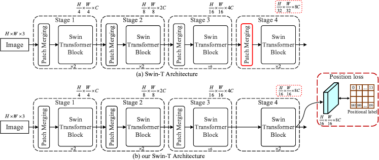
Figure 3: (a) The architecture of the original Swin Transformer (Swin-T); (b) The architecture of our modified Swin-T. This illustration was inspired by Swin-ViT figure 3(a).

3 Method

3.1 Absolute Positional Label

Here we take ViT-B Dosovitskiy et al. (2020) as an example, other ViT variants (e.g., Swin-B Liu et al. (2021)) are calculated in the same way. An overview of the absolute position as an auxiliary training task for classification is depicted in Figure 1.

We split an image $\mathsf{x}\in{{\mathbb{R}}^{H\times W\times C}}$ into fixed-size patches ${{\mathsf{x}}_{m}}\in{{\mathbb{R}}^{N\times({{m}^{2}}\cdot C)}}$, where $\left(H,W\right)$ is the resolution of the original image, $C$ is the number of channels, $\left(m,m\right)$ is the resolution of each image patch, and $N=HW/{{m}^{2}}$ is the number of generated patches. ${{\mathsf{x}}_{class}}$ is the classification token, whose state at the output of the $\mathsf{ViT}$ serves as the image representation ${{\mathsf{z}}_{class}}$ (Eq.2). In ViT-B, as an alternative to raw image patches, the input sequence can be formed from feature maps of a CNN He et al. (2016), the patch embedding projection $\mathsf{E}\in{{\mathbb{R}}^{({{m}^{2}}\cdot C)\times D}}$ is applied to patches extracted from a CNN feature map. The linear projection $\mathsf{E}$ maps $\mathsf{x}$ to $D$ dimensions. We refer to the output $\mathsf{y}$ of this projection as the patch embeddings:

$$\left[{{\mathsf{y}}_{class}};{{\mathsf{y}}_{1}}\mathsf{;}{{\mathsf{y}}_{2}};\cdots;{{\mathsf{y}}_{N}}\right]=\left[{{\mathsf{x}}_{class}};\mathsf{x}_{m}^{1}\mathsf{E;x}_{m}^{2}\mathsf{E;}\cdots\mathsf{;x}_{m}^{N}\mathsf{E}\right]$$ (1)

Feed the sequence of patch embeddings to a standard $\mathsf{ViT}$ encoder:

$$\left[{{\mathsf{z}}_{class}};{{\mathsf{z}}_{1}};{{\mathsf{z}}_{2}};\cdots{{\mathsf{z}}_{N}}\right]=\underset{\theta}{\mathop{\mathsf{ViT}}}\,\left(\left[{{\mathsf{y}}_{class}};{{\mathsf{y}}_{1}}\mathsf{;}{{\mathsf{y}}_{2}};\cdots;{{\mathsf{y}}_{N}}\right]\right)$$ (2)

where ${{\mathsf{z}}_{class}}$ is the image representation, which is input to the classifier to calculate the classification loss. $\theta$ denotes the trainable parameters of $\mathsf{ViT}$. ${{\mathsf{z}}_{i}}=\left({{\mathsf{z}}_{1}},\cdots,{{\mathsf{z}}_{N}}\right)$ is the representation of the image patch $\mathsf{x}_{m}^{i}=\left(\mathsf{x}_{m}^{1},\cdots,\mathsf{x}_{m}^{N}\right)$. We intercept half of ${{\mathsf{z}}_{i}}$, named $\frac{1}{2}{{\mathsf{z}}_{i}}$. Then use a trainable lightweight $\mathsf{MLP}$ block (shown in Figure 1) to project $\frac{1}{2}{{\mathsf{z}}_{i}}=\left(\frac{1}{2}{{\mathsf{z}}_{1}},\cdots,\frac{1}{2}{{\mathsf{z}}_{N}}\right)$ as the $d$-dimensional positional feature vector:

$$\left[{{\mathsf{p}}_{1}};{{\mathsf{p}}_{2}};\cdots;{{\mathsf{p}}_{N}}\right]=\mathsf{MLP}\left(\left[\frac{1}{2}{{\mathsf{z}}_{1}};\frac{1}{2}{{\mathsf{z}}_{2}};\cdots;\frac{1}{2}{{\mathsf{z}}_{N}}\right]\right)$$ (3)

The probability that ${{\mathsf{p}}_{i}}$ belongs to ${{{y}}_{i}}$ by SoftMax is:

$${{P}_{{{\mathsf{p}}_{i}},{{y}_{i}}}}=\frac{\exp(w_{{{y}_{i}}}^{\mathsf{T}}{{\mathsf{p}}_{i}})}{\sum\limits_{j=1}^{c}{\exp(w_{j}^{\mathsf{T}}{{\mathsf{p}}_{i}})}}$$ (4)

where $[{{\boldsymbol{w}}_{1}},\cdots,{{\boldsymbol{w}}_{c}}]\in{{R}^{d\times c}}$ is the weights in the positional classifier, $c$ denotes the number of classes (In ViT-B, $c=196$), and $d$ denotes the dimension of the feature. Each $\mathsf{x}_{m}^{i}$ corresponds to an absolute positional label ${{{y}}_{i}}=\left({{{y}}_{1}},\cdots,{{{y}}_{N}}\right)$, as shown in Figure 1 (${{{y}}_{1}}=\left(0\right),\cdots,{{{y}}_{9}}=\left(8\right)$). Absolute positional label trains the model by minimizing cross-entropy:

$${{L}_{p}}=-\frac{1}{n}\sum\limits_{i=1}^{n}{\log\left({{P}_{{{\mathsf{p}}_{i}},{{y}_{i}}}}\right)}$$ (5)

In the conventional classification task, we adopt the joint supervision of softmax loss and position loss to train the ViTs for discriminative feature learning. The formulation is given in Eq.6.

$$L={{L}_{s}}+\lambda{{L}_{p}}$$ (6)

where the scalar $\lambda$ is used for balancing the two loss functions.

3.2 Relative Positional Label

Besides the absolute position of each input image patch, we also consider the relative positional relationship between patches. Relative position methods encode the relative distance between input patches and learn the pairwise relationships of patches. We encode the relative position between the input image patches $\mathsf{x}_{m}^{i}$ and $\mathsf{x}_{m}^{j}$ into a vector $\mathsf{p}_{ij}^{r}$. To establish the pairwise positional relationship between the output image patch embeddings, we intercept half of ${{\mathsf{z}}_{i}}$, and combine them in pairs, as shown in Figure 2:

$${{\mathsf{z}}_{ij}}=concat\left(\frac{1}{2}{{\mathsf{z}}_{i}},\frac{1}{2}{{\mathsf{z}}_{j}}\right)$$ (7)

where the concat operation concatenates the two embeddings. Same as the absolute positional label, feed ${{\mathsf{z}}_{ij}}$ to a lightweight MLP block:

$$\mathsf{p}_{ij}^{r}=\mathsf{MLP}\left({{\mathsf{z}}_{ij}}\right)$$ (8)

where $\mathsf{p}_{ij}^{r}$ denotes the relative positional feature vector between $\mathsf{x}_{m}^{i}$ and $\mathsf{x}_{m}^{j}$ output by the model. We use the method in Swin-ViT Liu et al. (2021) to convert 2D absolute positional labels to 1D relative position labels ${{y}_{ij}}$. Similar to Eq.4 and 5, the optimization goal of the relative positional label is:

$$L_{p}^{r}=-\frac{1}{{{n}^{2}}}\sum\limits_{i=1}^{n}{\sum\limits_{j=1}^{n}{\log\left({{P}_{\mathsf{p}_{ij}^{r},{{y}_{ij}}}}\right)}}$$ (9)

In the conventional classification task, the relative position loss is trained in the same way as Eq.6.

3.3 Coupling Positional Label and MAE

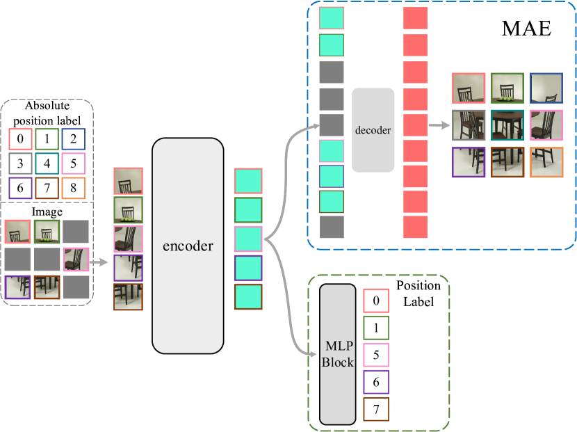
Figure 4: Our absolute positional label is combined with MAE. The output of the encoder is not only input to the decoder for MAE reconstruction of the image, but also to our positional label self-supervised MLP to output the absolute position of visible patches. This illustration was inspired by MAE.

The above two positional labels can not only be used as auxiliary supervision signals for classification tasks, but also can be used for self-supervised training of ViT, which can be combined with various current ViT self-supervised methods to obtain more powerful self-supervised signals, e.g., MAE He et al. (2021).

MAE masks a large random subset of image patches (e.g., 75%). A small subset of visible patches is then fed into the encoder. Mask tokens are introduced after the encoder, and the full set of encoded patches and mask tokens is processed by a small decoder that reconstructs the original image in pixels. This section illustrates our positional label combined with MAE, as shown in Figure 4. The output of the encoder is not only input to the decoder for MAE reconstruction of the image, but also to our positional label self-supervised MLP to output the absolute position of visible patches. Different from the original MAE, we do not add the encoder’s positional encoding during pre-training, and only use our positional labels for self-supervised training to fuse the positional information. Add the encoder’s positional encoding and use the proposed positional label, when fine-tuning the model.

3.4 Coupling Positional Label and Hierarchical ViT

Hierarchical ViT (e.g., Swin-ViT) to produce a hierarchical representation, the number of tokens is reduced by patch merging layers as the network gets deeper. The ”Stage 3” and ”Stage 4” of the original Swin-T, with output resolutions of $\frac{H}{16}\times\frac{W}{16}$ and $\frac{H}{32}\times\frac{W}{32}$, respectively, as shown in Figure 3(a). Taking the input image resolution of $224\times 224$ as an example, the sequence length of the encoded patches output by the original Swin-T is $\frac{224}{32}\times\frac{224}{32}=49$, which means that the number of classes of the positional label classification task $c=49$, much smaller than the number of classes of ViT-B ($c=196$), which we found experimentally that this affects the performance of positional label. In order to adapt to the positional label, we slightly modified the architecture of Swin-ViT and removed the last patch merging layer, so that the output resolution of Swin-T’s ”Stage 4” is $\frac{H}{16}\times\frac{W}{16}$, keeping the number of classes of the positional label classification task $c=196$, as shown in Figure 3(b). We found that this will not affect the performance of Swin-ViT, but it will increase the amount of calculation, which is also the limitation of the positional label in hierarchical ViT, and we will explore the solution to this problem in the next work. To efficiently incorporate positional labels, we use conditional positional encoding Chu et al. (2021) instead of the original relative positional bias. In the following experiments, we use the modified architecture for hierarchical ViT.

4 Experiments

We conduct experiments on ImageNet-1K Deng et al. (2009) image classification, Caltech-256 Griffin et al. (2007) and Mini-ImageNet Krizhevsky et al. (2012) small datasets image classification. In the following, we first conduct ablation experiments to demonstrate that positional encoding can be combined with the proposed positional labels, and then combine the proposed positional labels with the latest ViT architecture to demonstrate the effectiveness of the positional labels. Finally, we combine the proposed positional labels with MAE to demonstrate the potential of positional labels in self-supervised ViT training.

4.1 Experiment Settings

Dataset. For image classification, we benchmark the proposed positional label on the ImageNet-1K, which contains 1.28M training images and 50K validation images from 1,000 classes. To explore the performance of positional label on small datasets, we also conducted experiments on Caltech-256 and Mini-ImageNet. Caltech-256 has 257 classes with more than 80 images in each class. Mini-ImageNet contains a total of 60,000 images from 100 classes.

Implementation details. This setting mostly follows Liu et al. (2021). We use the PyTorch toolbox Paszke et al. (2019) to implement all our experiments. We employ an AdamW Kingma and Ba (2014) optimizer for 300 epochs using a cosine decay learning rate scheduler and 20 epochs of linear warm-up. A batch size of 256, an initial learning rate of 0.001, and a weight decay of 0.05 are used. ViT-B/16 uses an image size 384 and others use 224. We include most of the augmentation and regularization strategies of Liu et al. (2021) in training.

4.2 Ablation Studies

Table 1: Top-1 and Top-5 accuracies (%) for ViT-B model, on the ImageNet dataset. PE: positional encoding term of ViT; APL: the proposed absolute positional label; RPL: the proposed relative positional label.

Method	Top-1 acc.	Top-5 acc.
ViT-B + PE (Baseline)	77.91	92.48
ViT-B	76.34	90.83
ViT-B + APL	78.19	92.87
ViT-B + RPL	78.00	92.40
ViT-B + PE + RPL	79.07	93.67
ViT-B + PE + APL	79.11	93.73

Table 2: Top-1 and Top-5 accuracies (%) for Swin-T model, on the ImageNet dataset.

Method	Top-1 acc.	Top-5 acc.
Swin-T + PE (Baseline)	81.32	95.64
Swin-T	80.14	94.93
Swin-T + APL	80.89	95.17
Swin-T + RPL	81.15	95.30
Swin-T + PE + RPL	81.93	95.67
Swin-T + PE + APL	81.51	95.83

Positional encoding. Incorporating explicit representations of positional information is known to be especially important for Transformers, since the model is otherwise entirely invariant to sequence ordering, which is undesirable for modeling structured data. Experiments show that our proposed positional label can completely replace positional encoding to add positional information to the ViT model. Surprisingly, we found that the proposed positional label can be used in combination with conventional positional encoding, the model does not learn an identity and can achieve the best performance gain. We experiment on ViT-B and Swin-T, as shown in Table 1 and Table 2.

Figure 5: Illustration of position loss with different $\lambda$, using the ViT-B architecture.

Hyperparameter $\lambda$. The hyperparameter $\lambda$ balances the classification loss and position loss. It is essential to our model. So we conduct an experiment to investigate the sensitiveness of this parameter. In our experiments, we vary $\lambda$ from 0 to 1.25 to learn different models. The Top-1 accuracies of these models on the ImageNet-1K dataset are shown in Figure 5. Properly choosing the value of $\lambda$ can improve the accuracy of the models. We also observe that the performance of the models remains largely stable across a wide range of $\lambda$. All experiments in this paper set $\lambda=0.5$.

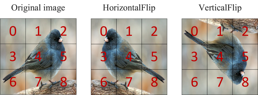
Figure 6: Data augmentation. Our positional label works with different image augmentations.

Data augmentation. Because the data augmentation affects our positional labels, as shown in Figure 6, the image uses different data augmentations, and the bird head corresponds to different positional labels. Left: positional label is 2. Middle: positional label is 0. Right: positional label is 8. Table 3 studies the influence of data augmentation on our positional label. Using random horizontal flipping for our positional label improves the performance, but combining random horizontal flipping and random vertical flipping has little effect on the results, suggesting that positional label does not require large augmentation to regularize training.

Table 3: Data augmentation. Our positional label works with minimal augmentation, using the ViT-B architecture. crop: random resized crop; RHF: random horizontal flipping; RVF: random vertical flipping.

Method	Top-1 acc.	Top-5 acc.
crop + RHF (Baseline)	77.91	92.48
crop + APL	78.54	93.13
crop + RPL	78.26	92.95
crop + RHF + APL	79.11	93.73
crop + RHF + RPL	79.07	93.67
crop + RHF + RVF + APL	79.09	93.69
crop + RHF + RVF + RPL	79.10	92.87

4.3 Image Classification on the ImageNet-1K

Table 4: Top-1 and Top-5 accuracies (%) of different ViT backbones, on the ImageNet dataset. Each ViT variant follows the approach of adding positional encoding in its paper.

Method	Top-1 acc.	Top-5 acc.
ViT-B Dosovitskiy et al. (2020)	77.91	92.48
DeiT-B Touvron et al. (2021)	81.87	93.92
Swin-B Liu et al. (2021)	83.35	96.38
NesT-B Zhang et al. (2022)	83.67	96.16
ViT-B + APL	79.11	93.73
DeiT-B + APL	82.49	94.34
Swin-B + APL	83.76	96.83
NesT-B + APL	84.13	96.85
ViT-B + RPL	79.07	93.67
DeiT-B + RPL	82.85	94.21
Swin-B + RPL	84.09	96.77
NesT-B + RPL	83.93	96.81

We combine absolute and relative positional labels with various ViT variants, each ViT variant follows the approach of adding positional encoding in its paper. The experimental results show that the proposed positional label can significantly improve the performance of ViT, as shown in Table 4: +1.20% for ViT-B with the absolute positional label (79.11%) over ViT-B (77.91%), and +0.74% for Swin-B with the relative positional label (84.09%) over Swin-B (83.35%). The experimental results show that the performance improvement of positional labels for the full-attention transformer (e.g., ViT-B) is higher than that of the local-attention transformer (e.g., Swin-B), which also indicates that the local-attention transformer can process limited data more efficiently.

In the classification task, we use a classification loss function combined with our positional labels for joint training. We observe the classification loss changing curve of ViT and find an interesting phenomenon that the classification loss of ViT with positional labels is smaller (as shown in Figure 7), which indicates that our positional labels can benefit the convergence of ViT.

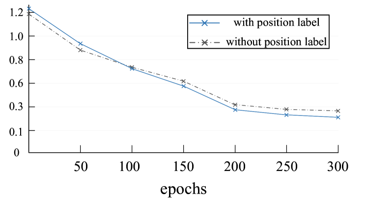
Figure 7: During training, the classification loss of ViT-B with the positional label and ViT-B without the positional label.

Table 5: Top-1 and Top-5 accuracies (%) of various ViT variants, on the Mini-ImageNet dataset.

Method	Top-1 acc.	Top-5 acc.
ViT-B Dosovitskiy et al. (2020)	58.28	79.57
DeiT-B Touvron et al. (2021)	63.67	83.92
Swin-B Liu et al. (2021)	67.39	86.88
NesT-B Zhang et al. (2022)	67.43	86.75
ViT-B + APL	64.43	83.73
DeiT-B + APL	66.49	85.34
Swin-B + APL	68.91	87.83
NesT-B + APL	68.73	87.95
ViT-B + RPL	63.97	83.06
DeiT-B + RPL	66.85	85.21
Swin-B + RPL	69.11	88.02
NesT-B + RPL	69.56	88.67

4.4 Image Classification on Caltech-256 and Mini-ImageNet

We show the performance of ViT on small datasets in Table 5 and Table 6. It is known that ViTs usually perform poorly on such tasks as they typically require large datasets to be trained on. The models that perform well on large-scale ImageNet do not necessary work perform on small-scale Mini-ImageNet and Caltech-256, e.g., ViT-B has top-1 accuracy of 58.28% and Swin-B has top-1 accuracy of 67.39% on the Mini-ImageNet, which suggests that ViTs are more challenging to train with less data. Our proposed positional label can accelerate the convergence of ViT and significantly improve the performance of ViT on small datasets like Mini-ImageNet and Caltech-256. On Mini-ImageNet, the top-1 accuracy of ViT-B and Swin-B are improved by 6.15% and 1.72%, respectively. On Caltech-256, the top-1 accuracy of ViT-B and Swin-B are improved by 3.16% and 2.24%, respectively.

Table 6: Top-1 and Top-5 accuracies (%) of various ViT variants, on Caltech-256 dataset.

Method	Top-1 acc.	Top-5 acc.
ViT-B Dosovitskiy et al. (2020)	37.57	56.83
DeiT-B Touvron et al. (2021)	40.56	61.24
Swin-B Liu et al. (2021)	46.67	67.22
NesT-B Zhang et al. (2022)	45.54	66.35
ViT-B + APL	40.73	60.63
DeiT-B + APL	41.79	62.86
Swin-B + APL	48.91	68.33
NesT-B + APL	49.77	68.84
ViT-B + RPL	40.51	61.07
DeiT-B + RPL	41.28	61.56
Swin-B + RPL	48.80	68.09
NesT-B + RPL	48.97	67.99

4.5 Coupling Positional Label and MAE

Table 7: Experimental results of positional label combined with MAE on the ImageNet-1K. Pre-trained for 400 epochs.

Method	Top-1 acc.
ViT-B Dosovitskiy et al. (2020)	77.91
ViT-B + MAE He et al. (2021)	79.54
ViT-B + MAE + APL	80.40
ViT-B + MAE + RPL	80.21

We do self-supervised pre-training on the ImageNet-1K training set. Then we do supervised training to evaluate the representations with end-to-end fine-tuning. We report top-1 validation accuracy. This experiment uses ViT-B as the backbone, and the experimental setting follows the default setting of MAE He et al. (2021). Table 7 is a comparison between ViT-B trained from scratch vs. fine-tuned from MAE with our positional label.

MAE finds that masking a high proportion of the input image, e.g., 75%, yields a nontrivial and meaningful self-supervisory task. Random sampling with a high masking ratio largely eliminates redundancy, thus creating a task that cannot be easily solved by extrapolation from visible neighboring patches. We find that this also applies to our proposed positional label, where the encoder uses a small subset of visible patches to reconstruct the overall positional information of the image, yielding a more powerful self-supervised signal. As shown in Figure 8, the training difficulty of the model increases as the masking ratio increases.

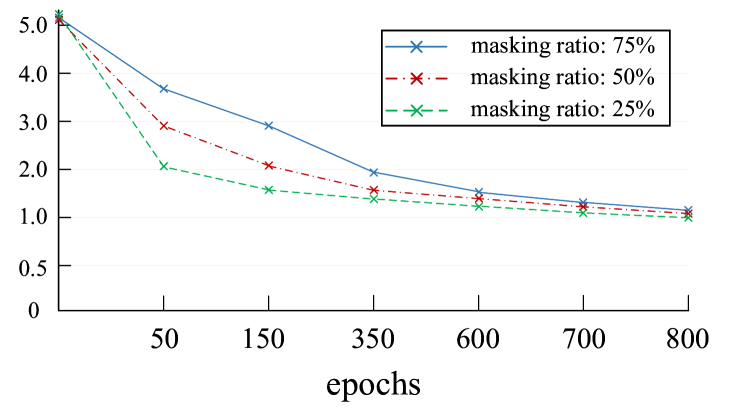
Figure 8: The position loss with different masking ratios.

Under this design, MAE and our positional label can achieve a win-win scenario: MAE reconstructs clear masked patch pixels that help the positional loss capture the overall positional information of the image, while the positional loss also incorporates the positional information into the MAE reconstruction, allowing the model to consider the overall structure of the image during the reconstruction process.

5 Conclusions

In this paper, we propose two positional labels for self-supervised training of ViT. The extensive experiments show that our method can be combined with various ViT variants, bringing significant improvements on classification tasks. Our methods could be easily plugged into self-attention layers. In addition, our positional labels can also be used for ViT fully self-supervised methods to provide a powerful self-supervised signal.

References

- Caron et al. [2020] Mathilde Caron, Ishan Misra, Julien Mairal, Priya Goyal, Piotr Bojanowski, and Armand Joulin. Unsupervised learning of visual features by contrasting cluster assignments. In H. Larochelle, M. Ranzato, R. Hadsell, M.F. Balcan, and H. Lin, editors, Advances in Neural Information Processing Systems, volume 33, pages 9912–9924. Curran Associates, Inc., 2020.
- Caron et al. [2021] Mathilde Caron, Hugo Touvron, Ishan Misra, Hervé Jégou, Julien Mairal, Piotr Bojanowski, and Armand Joulin. Emerging properties in self-supervised vision transformers. In Proceedings of the IEEE/CVF International Conference on Computer Vision (ICCV), pages 9650–9660, October 2021.
- Chen et al. [2020] Mark Chen, Alec Radford, Rewon Child, Jeffrey Wu, Heewoo Jun, David Luan, and Ilya Sutskever. Generative pretraining from pixels. In Hal Daumé III and Aarti Singh, editors, Proceedings of the 37th International Conference on Machine Learning, volume 119 of Proceedings of Machine Learning Research, pages 1691–1703. PMLR, 13–18 Jul 2020.
- Chen et al. [2021] Xinlei Chen, Saining Xie, and Kaiming He. An empirical study of training self-supervised vision transformers. In Proceedings of the IEEE/CVF International Conference on Computer Vision (ICCV), pages 9640–9649, October 2021.
- Chu et al. [2021] Xiangxiang Chu, Bo Zhang, Zhi Tian, Xiaolin Wei, and Huaxia Xia. Do we really need explicit position encodings for vision transformers? CoRR, abs/2102.10882, 2021.
- Dai et al. [2019] Zihang Dai, Zhilin Yang, Yiming Yang, Jaime G. Carbonell, Quoc V. Le, and Ruslan Salakhutdinov. Transformer-xl: Attentive language models beyond a fixed-length context. CoRR, abs/1901.02860, 2019.
- Deng et al. [2009] Jia Deng, Wei Dong, Richard Socher, Li-Jia Li, Kai Li, and Li Fei-Fei. Imagenet: A large-scale hierarchical image database. In 2009 IEEE Conference on Computer Vision and Pattern Recognition, pages 248–255, 2009.
- Devlin et al. [2018] Jacob Devlin, Ming-Wei Chang, Kenton Lee, and Kristina Toutanova. BERT: pre-training of deep bidirectional transformers for language understanding. CoRR, abs/1810.04805, 2018.
- Dosovitskiy et al. [2020] Alexey Dosovitskiy, Lucas Beyer, Alexander Kolesnikov, Dirk Weissenborn, Xiaohua Zhai, Thomas Unterthiner, Mostafa Dehghani, Matthias Minderer, Georg Heigold, Sylvain Gelly, Jakob Uszkoreit, and Neil Houlsby. An image is worth 16x16 words: Transformers for image recognition at scale. CoRR, abs/2010.11929, 2020.
- Gehring et al. [2017] Jonas Gehring, Michael Auli, David Grangier, Denis Yarats, and Yann N. Dauphin. Convolutional sequence to sequence learning. In Doina Precup and Yee Whye Teh, editors, Proceedings of the 34th International Conference on Machine Learning, volume 70 of Proceedings of Machine Learning Research, pages 1243–1252. PMLR, 06–11 Aug 2017.
- Griffin et al. [2007] Gregory Griffin, Alex Holub, and Pietro Perona. Caltech-256 object category dataset. 2007.
- He et al. [2016] Kaiming He, Xiangyu Zhang, Shaoqing Ren, and Jian Sun. Deep residual learning for image recognition. In Proceedings of the IEEE Conference on Computer Vision and Pattern Recognition (CVPR), June 2016.
- He et al. [2021] Kaiming He, Xinlei Chen, Saining Xie, Yanghao Li, Piotr Dollár, and Ross B. Girshick. Masked autoencoders are scalable vision learners. CoRR, abs/2111.06377, 2021.
- Kingma and Ba [2014] Diederik P Kingma and Jimmy Ba. Adam: A method for stochastic optimization. arXiv preprint arXiv:1412.6980, 2014.
- Krizhevsky et al. [2012] Alex Krizhevsky, Ilya Sutskever, and Geoffrey E Hinton. Imagenet classification with deep convolutional neural networks. Advances in neural information processing systems, 25:1097–1105, 2012.
- Li et al. [2018] Chen Li, Zhen Zhang, Wee Sun Lee, and Gim Hee Lee. Convolutional sequence to sequence model for human dynamics. In Proceedings of the IEEE Conference on Computer Vision and Pattern Recognition (CVPR), June 2018.
- Liu et al. [2021] Ze Liu, Yutong Lin, Yue Cao, Han Hu, Yixuan Wei, Zheng Zhang, Stephen Lin, and Baining Guo. Swin transformer: Hierarchical vision transformer using shifted windows. In Proceedings of the IEEE/CVF International Conference on Computer Vision (ICCV), pages 10012–10022, October 2021.
- Paszke et al. [2019] Adam Paszke, Sam Gross, Francisco Massa, Adam Lerer, James Bradbury, Gregory Chanan, Trevor Killeen, Zeming Lin, Natalia Gimelshein, Luca Antiga, et al. Pytorch: An imperative style, high-performance deep learning library. Advances in neural information processing systems, 32:8026–8037, 2019.
- Ramachandran et al. [2019] Prajit Ramachandran, Niki Parmar, Ashish Vaswani, Irwan Bello, Anselm Levskaya, and Jon Shlens. Stand-alone self-attention in vision models. In H. Wallach, H. Larochelle, A. Beygelzimer, F. d'Alché-Buc, E. Fox, and R. Garnett, editors, Advances in Neural Information Processing Systems, volume 32. Curran Associates, Inc., 2019.
- Sameni et al. [2022] Sepehr Sameni, Simon Jenni, and Paolo Favaro. Dilemma: Self-supervised shape and texture learning with transformers. arXiv preprint arXiv:2204.04788, 2022.
- Shaw et al. [2018] Peter Shaw, Jakob Uszkoreit, and Ashish Vaswani. Self-attention with relative position representations. CoRR, abs/1803.02155, 2018.
- Srinivas et al. [2021] Aravind Srinivas, Tsung-Yi Lin, Niki Parmar, Jonathon Shlens, Pieter Abbeel, and Ashish Vaswani. Bottleneck transformers for visual recognition. In Proceedings of the IEEE/CVF Conference on Computer Vision and Pattern Recognition (CVPR), pages 16519–16529, June 2021.
- Touvron et al. [2021] Hugo Touvron, Matthieu Cord, Matthijs Douze, Francisco Massa, Alexandre Sablayrolles, and Herve Jegou. Training data-efficient image transformers-amp; distillation through attention. In Marina Meila and Tong Zhang, editors, Proceedings of the 38th International Conference on Machine Learning, volume 139 of Proceedings of Machine Learning Research, pages 10347–10357. PMLR, 18–24 Jul 2021.
- Vaswani et al. [2017] Ashish Vaswani, Noam Shazeer, Niki Parmar, Jakob Uszkoreit, Llion Jones, Aidan N Gomez, Ł ukasz Kaiser, and Illia Polosukhin. Attention is all you need. In I. Guyon, U. Von Luxburg, S. Bengio, H. Wallach, R. Fergus, S. Vishwanathan, and R. Garnett, editors, Advances in Neural Information Processing Systems, volume 30. Curran Associates, Inc., 2017.
- Wang et al. [2019] Alex Wang, Yada Pruksachatkun, Nikita Nangia, Amanpreet Singh, Julian Michael, Felix Hill, Omer Levy, and Samuel Bowman. Superglue: A stickier benchmark for general-purpose language understanding systems. In H. Wallach, H. Larochelle, A. Beygelzimer, F. d'Alché-Buc, E. Fox, and R. Garnett, editors, Advances in Neural Information Processing Systems, volume 32. Curran Associates, Inc., 2019.
- Wu et al. [2021] Kan Wu, Houwen Peng, Minghao Chen, Jianlong Fu, and Hongyang Chao. Rethinking and improving relative position encoding for vision transformer. In Proceedings of the IEEE/CVF International Conference on Computer Vision (ICCV), pages 10033–10041, October 2021.
- Zhang et al. [2022] Zizhao Zhang, Han Zhang, Long Zhao, Ting Chen, Sercan O Arik, and Tomas Pfister. Nested hierarchical transformer: Towards accurate, data-efficient and interpretable visual understanding. In AAAI Conference on Artificial Intelligence (AAAI), volume 2022, 2022.
- Zhao et al. [2020] Hengshuang Zhao, Jiaya Jia, and Vladlen Koltun. Exploring self-attention for image recognition. In Proceedings of the IEEE/CVF Conference on Computer Vision and Pattern Recognition (CVPR), June 2020.