Convolutional layers are equivariant to discrete shifts
but not continuous translations
Abstract
The purpose of this short and simple note is to clarify a common misconception about convolutional neural networks (CNNs). CNNs are made up of convolutional layers which are shift equivariant due to weight sharing. However, convolutional layers are not translation equivariant, even when boundary effects are ignored and when pooling and subsampling are absent. This is because shift equivariance is a discrete symmetry while translation equivariance is a continuous symmetry. This fact is well known among researchers in equivariant machine learning, but is usually overlooked among non-experts. To minimize confusion, we suggest using the term ‘shift equivariance’ to refer to discrete shifts in pixels and ‘translation equivariance’ to refer to continuous translations.
1 Continuous vs discrete equivariance
A convolution is a linear operator of two functions and . In one dimension, is
| (1) |
An operator is equivariant to a transformation if (Cohen & Welling, 2016)
| (2) |
is equivariant to the transformation ; this is called translation equivariance.
Convolutional layers are the building blocks of convolutional neural networks (CNNs) (Zhang et al., 1990; LeCun et al., 1989). Convolutional layers perform a discrete convolution followed by a nonlinearity (LeCun et al., 1995). We denote discrete operators and functions with the superscript and indices with a subscript. A discrete convolution in 1D can be written as
| (3) |
A discrete convolution is equivariant to the transformation ; this is called shift equivariance (Fukushima & Miyake, 1982; Bronstein et al., 2021; Cohen & Welling, 2016). If the nonlinearity is also shift equivariant, then the convolutional layer will be shift equivariant, ignoring boundary effects (Azulay & Weiss, 2018; Kayhan & Gemert, 2020; Zhang, 2019; Chaman & Dokmanic, 2021).
We now show that these layers are not translation equivariant. The essence of the argument is that translation equivariance is a property of continuous systems, while convolutional layers operate on discrete models that do not have a continuous symmetry.
The data from the real-world system is a continuous function. To map from the continuous system to the discrete model, we introduce a discretization operator , where . In general, it is not possible to map from the discrete model back to the continuous system. Applying a convolutional layer to the continuous data can thus be written as where is the nonlinearity and is the convolutional kernel. By the definition of equivariance in eq. 2, the convolutional layer is translation equivariant if
| (4) |
where is the transformation for . The left hand side of eq. 4 is well-defined; it involves translating by , discretizing , then performing the convolution and nonlinearity. However, the right hand side of eq. 4 is not well-defined; it requires translating a discrete quantity by a continuous amount. Therefore, eq. 4 cannot possibly be true, meaning that convolutional layers are not translation equivariant.
Strictly speaking, it is possible to define a discrete translation which translates discrete data by a non-integer number of pixels. A discrete translation could be defined, for example, by interpolating the discrete data between gridpoints, translating the interpolated data, then discretizing the result. Nevertheless, it is is impossible to design discrete systems that have an exact continuous translation equivariance, i.e.,
| (5) |
because information about the continuous function is lost in the discretization process. It is possible to design discrete convolutions that do not change significantly (i.e., are Lipschitz continuous) to perturbations of the input (Bruna & Mallat, 2013).
2 Intuition
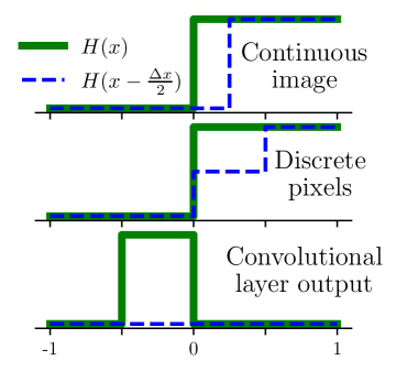
We consider a simple example of an image in 1D. Suppose our image domain is and our 1D image is the Heaviside step function where
Now suppose we discretize (i.e., ‘take a picture of’) our image using a discretization operator which computes the average value of the image inside the th pixel for . This means that , where are the pixel boundaries and . The image has pixels. Suppose also that our convolutional layer performs a convolution with kernel and bias followed by a ReLU nonlinearity; this layer is designed to detect edges in the image.
Now, let us compare the output of the convolutional layer between the image and a translated image . The original image pixels are , while the translated image pixels are . As illustrated in fig. 1, the output of the convolutional layer on the original image is while the output of the convolutional layer on the translated image is . The convolutonal layer detects an edge in the first image, but does not detect an edge in the translated image. This example demonstrates intuitively the point of this paper: that convolutional layers are equivariant to discrete shifts in pixels, but not equivariant to continuous translations in images.
References
- Azulay & Weiss (2018) Aharon Azulay and Yair Weiss. Why do deep convolutional networks generalize so poorly to small image transformations? arXiv preprint arXiv:1805.12177, 2018.
- Bronstein et al. (2021) Michael M Bronstein, Joan Bruna, Taco Cohen, and Petar Veličković. Geometric deep learning: Grids, groups, graphs, geodesics, and gauges. arXiv preprint arXiv:2104.13478, 2021.
- Bruna & Mallat (2013) Joan Bruna and Stéphane Mallat. Invariant scattering convolution networks. IEEE transactions on pattern analysis and machine intelligence, 35(8):1872–1886, 2013.
- Chaman & Dokmanic (2021) Anadi Chaman and Ivan Dokmanic. Truly shift-invariant convolutional neural networks. In Proceedings of the IEEE/CVF Conference on Computer Vision and Pattern Recognition, pp. 3773–3783, 2021.
- Cohen & Welling (2016) Taco Cohen and Max Welling. Group equivariant convolutional networks. In International conference on machine learning, pp. 2990–2999. PMLR, 2016.
- Fukushima & Miyake (1982) Kunihiko Fukushima and Sei Miyake. Neocognitron: A self-organizing neural network model for a mechanism of visual pattern recognition. In Competition and cooperation in neural nets, pp. 267–285. Springer, 1982.
- Kayhan & Gemert (2020) Osman Semih Kayhan and Jan C van Gemert. On translation invariance in cnns: Convolutional layers can exploit absolute spatial location. In Proceedings of the IEEE/CVF Conference on Computer Vision and Pattern Recognition, pp. 14274–14285, 2020.
- LeCun et al. (1989) Yann LeCun, Bernhard Boser, John S Denker, Donnie Henderson, Richard E Howard, Wayne Hubbard, and Lawrence D Jackel. Backpropagation applied to handwritten zip code recognition. Neural computation, 1(4):541–551, 1989.
- LeCun et al. (1995) Yann LeCun, Yoshua Bengio, et al. Convolutional networks for images, speech, and time series. The handbook of brain theory and neural networks, 3361(10):1995, 1995.
- Zhang (2019) Richard Zhang. Making convolutional networks shift-invariant again. In International conference on machine learning, pp. 7324–7334. PMLR, 2019.
- Zhang et al. (1990) Wei Zhang, Kazuyoshi Itoh, Jun Tanida, and Yoshiki Ichioka. Parallel distributed processing model with local space-invariant interconnections and its optical architecture. Applied optics, 29(32):4790–4797, 1990.