Refining neural network predictions using background knowledge

Abstract

Recent work has shown logical background knowledge can be used in learning systems to compensate for a lack of labeled training data. Many methods work by creating a loss function that encodes this knowledge. However, often the logic is discarded after training, even if it is still useful at test time. Instead, we ensure neural network predictions satisfy the knowledge by refining the predictions with an extra computation step. We introduce differentiable refinement functions that find a corrected prediction close to the original prediction. We study how to effectively and efficiently compute these refinement functions. Using a new algorithm called Iterative Local Refinement (ILR), we combine refinement functions to find refined predictions for logical formulas of any complexity. ILR finds refinements on complex SAT formulas in significantly fewer iterations and frequently finds solutions where gradient descent can not. Finally, ILR produces competitive results in the MNIST addition task.

1 Introduction

Recent years have shown promising examples of using symbolic background knowledge in learning systems: From training classifiers with weak supervision signals Manhaeve et al. (2018), generalizing learned classifiers to new tasks Roychowdhury et al. (2021), compensating for a lack of good supervised data Diligenti et al. (2017); Donadello et al. (2017), to enforcing the structure of outputs through a logical specification Xu et al. (2018). The main idea underlying these integrations of learning and reasoning, often called neuro-symbolic integration, is that background knowledge can complement the neural network when one lacks high-quality labeled data Giunchiglia et al. (2022b). Although pure deep learning approaches excel when learning over vast quantities of data with gigantic amounts of compute Chowdhery et al. (2022); Ramesh et al. (2022), most tasks are not afforded this luxury.

Many neuro-symbolic methods work by creating a differentiable loss function that encodes the background knowledge (Figure 1a). However, often the logic is discarded after training, even though this background knowledge could still be helpful at test time Roychowdhury et al. (2021); Giunchiglia et al. (2022a). Instead, we ensure we constrain the neural network with the background knowledge, both during train time and test time, by correcting its output such that it will satisfy the background knowledge (Figure 1b). In particular, we consider how to make such corrections while being as close as possible to the original predictions of the neural network.

We study how to effectively and efficiently correct the neural network by ensuring its predictions satisfy the symbolic background knowledge. In particular, we consider fuzzy logics formed using functions called t-norms Klement et al. (2013); Ross (2010). Prior work has shown how to use a gradient ascent-based optimization procedure to find a prediction that satisfies this fuzzy background knowledge Diligenti et al. (2017); Roychowdhury et al. (2021). However, a recent model called KENN Daniele and Serafini (2019) shows how to compute the correction analytically for a fragment of the Gödel logic.

To extend this line of work, we introduce the concept of refinement functions, and derive refinement functions for many fuzzy logic operators. Refinement functions are functions that find a prediction that satisfies the background knowledge while staying close to the neural network’s original prediction. Using a new algorithm called Iterative Local Refinement (ILR), we can combine refinement functions for different fuzzy logic operators to efficiently find refinements for logical formulas of any complexity. Since refinement functions are differentiable, we can easily integrate them as a neural network layer. In our experiments, we compare ILR with an approach using gradient ascent. We find that ILR finds optimal refinements in significantly fewer iterations. Moreover, ILR often produces results that stay closer to the original predictions or better satisfy the background knowledge. Finally, we evaluated ILR on the MNIST Addition task Manhaeve et al. (2018) and show that ILR can be combined with neural networks to solve common neuro-symbolic tasks.

In summary, our contributions are:

1. We formalize the concept of minimal refinement functions in Section 4.

2. We introduce the ILR algorithm in Section 5, which uses the minimal refinement functions for individual fuzzy operators to find refinements for general logical formulas.

3. We discuss how to use ILR for neuro-symbolic AI in Section 6, where we exploit the fact that ILR is a differentiable algorithm.

4. We analytically derive minimal refinement functions for individual fuzzy operators constructed from the Gödel, Łukasiewicz, and product t-norms in Section 7.2.

5. We discuss a large class of t-norms for which we can analytically derive minimal refinement functions in Section 7.

6. We compare ILR to gradient descent approaches and show it finds refinements on complex SAT formulas in significantly fewer iterations and frequently finds solutions where gradient descent can not.

7. We apply ILR to the MNIST Addition task Manhaeve et al. (2018) to test how ILR behaves when injecting knowledge into neural network models.

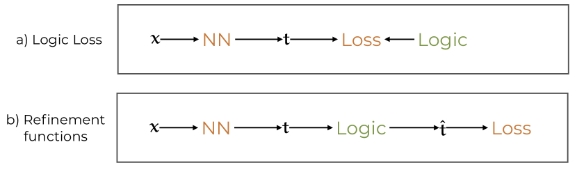
Figure 1: Comparing different approaches for constraining neural networks with background knowledge. Loss-based approaches include LTN, SBR, and Semantic Loss, while KENN, C-HMCNN(h), and SBR-CC are representatives for refinement functions.

2 Related work

ILR falls into a larger body of work that attempts to integrate background knowledge expressed as logical formulas into neural networks. For an overview, see Giunchiglia et al. (2022b). As shown in Figure 1, methods can be categorized by whether they only use background knowledge during training in the form of a loss function Badreddine et al. (2022); Xu et al. (2018); Diligenti et al. (2017); Fischer et al. ; Yang et al. ; van Krieken et al. (2022) or whether the background knowledge is part of the model and therefore enforces the knowledge also at test time Daniele and Serafini (2019); Wang et al. (2019); Giunchiglia and Lukasiewicz (2021); Ahmed et al. (2022); Hoernle et al. (2022); Dragone et al. . ILR is a method in the second category. We note that these approaches can be combined Giunchiglia et al. (2022a); Roychowdhury et al. (2021).

First, we discuss approaches that construct loss functions from the logical formulas (Figure 1a). These loss functions measure when the deep learning model violates the background knowledge, such that minimizing the loss function amounts to “correcting” such violations van Krieken et al. (2022). While these methods show significant empirical improvement, they do not guarantee that the neural network will satisfy the formulas outside the training data. LTN and SBR Badreddine et al. (2022); Diligenti et al. (2017) use fuzzy logic to provide compatibility with neural network learning, while Semantic Loss Xu et al. (2018) uses probabilistic logics. The formalization of refinement functions can be extended to probabilistic logics by defining a suitable notion of minimality, like the KL-divergence between the original and refined distributions over ground atoms.

Among the methods where knowledge is part of the model, KENN inspired ILR Daniele and Serafini (2019, 2022). KENN is a framework that injects knowledge into neural networks by iteratively refining its predictions. It uses a relaxed version of the Gödel t-conorm obtained through a relaxation of the argmax function, which it applies in logit space. Closely related to both ILR and KENN is C-HMCNN(h) Giunchiglia and Lukasiewicz (2021), which we see as computing the minimal refinement function for stratified normal logic programs under Gödel t-norm semantics. We discuss this connection in more detail in Section 7.2.1.

The loss-function based method SBR also introduces a procedure for using the logical formulas at test time in the context of collective classification Diligenti et al. (2017); Roychowdhury et al. (2021). Unlike KENN Daniele and Serafini (2019), these approaches do not enforce the background knowledge during training but only use it as a test time procedure. In particular, Roychowdhury et al. (2021) shows that doing these corrections at test time improves upon just using the loss-function approach. Unlike our analytic approach to refinement functions, SBR finds new predictions using a gradient descent procedure very similar to the algorithm we discuss in Section 9.1.2. We show it is much slower to compute than ILR.

Another method closely related to ILR is the neural network layer SATNet Wang et al. (2019), which has a setup closely related to ours. However, SATNet does not have a notion like minimality and uses a different underlying logic constructed from a semidefinite relaxation. DeepProbLog Manhaeve et al. (2018) also is a probabilistic logic, but unlike Semantic Loss is used to derive new statements through proofs and cannot directly be used to correct the neural network on predictions that do not satisfy the background knowledge. Instead, ILR can be used both for injecting constraints on the output of a neural network, as well as for proving new statements starting from the neural network predictions.

Finally, some methods are limited to equality and inequality constraints rather than general symbolic background knowledge Fischer et al. ; Hoernle et al. (2022). DL2 Fischer et al. combines these constraints into a real-valued loss function, while MultiplexNet Hoernle et al. (2022) adds the knowledge as part of the model. However, MultiplexNet requires expressing the logical formulas as a DNF formula, which is hard to scale.

3 Fuzzy Operators

We will first provide the necessary background knowledge for defining and analyzing minimal refinement functions. In particular, we will consider fuzzy operators, which generalize the connectives of classical boolean logic. For formal treatments of the study of such operators, we refer the reader to Klement et al. (2013), which discusses t-norms and t-conorms, to Jayaram and Baczynski (2008) for fuzzy implications, to Calvo et al. (2002) for aggregation functions, and to van Krieken et al. (2022) for an analysis of the derivatives of these operators.

Name	T-norm
Minimum	${T_{G}}({\bm{t}})=\min_{i=1}^{n}t_{i}$
Product	${T_{P}}({\bm{t}})=\prod_{i=1}^{n}t_{i}$
Łukasiewicz	${T_{L}}({\bm{t}})=\max(\sum_{i=1}^{n}t_{i}-(n-1),0)$

Table 1: Some common t-norms extended to any-arity aggregation operators.

Definition 1.

A function $T:[0,1]^{2}\rightarrow[0,1]$ is a t-norm (triangular norm) if it is commutative, associative, increasing in both arguments, and if for all $t\in[0,1]$, $T(1,t)=t$.

Similarly, a function $S:[0,1]^{2}\rightarrow[0,1]$ is a t-conorm if the last condition instead is that for all $t\in[0,1]$, $S(0,t)=t$.

Dual t-conorms are formed from a t-norm $T$ using $S(t_{1},t_{2})=1-T(1-t_{1},1-t_{2})$. We list any-arity extensions, constructed using $T({\bm{t}})=T(t_{1},T({\bm{t}}_{2:n}))$, $T(t_{i})=t_{i}$ of five basic t-norms in Table 1. Here ${\bm{t}}=[t_{1},...,t_{n}]^{\top}\in[0,1]^{n}$ is a vector of fuzzy truth values, which we will often refer to as (truth) vectors. These any-arity extensions are examples of fuzzy aggregation operators Calvo et al. (2002).

Definition 2.

A t-norm $T$ is Archimedean if for all $x,y\in(0,1)$, there is an $n$ such that $T(\underbrace{x,\dots,x}_{n\times})<y$.

A continuous t-norm $T$ is strict if, in addition, for all $x\in(0,1)$, $0<T(x,x)<x$.

Definition 3.

A function $I:[0,1]^{2}\rightarrow[0,1]$ is a fuzzy implication if for all $t_{1},t_{2}\in[0,1]$, $I(\cdot,t_{2})$ is decreasing, $I(t_{1},\cdot)$ is increasing and if $I(0,0)=1$, $I(1,1)=1$ and $I(1,0)=0$.

Note that fuzzy implications do not have $n$-ary extensions as they are not associative. The so-called S-implications are formed from the t-conorm by generalizing the material implication using $I(a,c)=S(1-a,c)$. Furthermore, every t-norm induces a unique residuum or R-implication Jayaram and Baczynski (2008) $R_{T}(a,c)=\sup\{z|T(z,a)\leq c\}$.

Logical formulas $\varphi$ can be evaluated using compositions of fuzzy operators. We assume $\varphi$ is a propositional logic formula, but note this evaluation procedure can be extended to grounded first-order logical formulas on finite domains. For instance, Daniele and Serafini (2022) introduced a technique for propositionalizing universally quantified formulas of predicate logic in the context of KENN. Moreover, this technique can be extended to existential quantification by treating it as a disjunction. We assume a set of propositions ${\mathcal{P}}=\{P_{1},...,P_{n}\}$ and constants ${\mathcal{C}}=\{C_{1},...,C_{m}\}$, where each constant has a fixed value $C_{i}\in[0,1]$.

Definition 4.

If $T$ is a t-norm, $S$ a t-conorm and $I$ a fuzzy implication, then the fuzzy evaluation operator $f_{\varphi}:[0,1]^{n}\rightarrow[0,1]$ of the formula $\varphi$ with propositions ${\mathcal{P}}$ and constants ${\mathcal{C}}$ is a function of truth vectors ${\bm{t}}$ and given as

$$f_{P_{i}}({\bm{t}}) =t_{i}$$ (1)

$$f_{C_{j}}({\bm{t}}) =C_{j}$$ (2)

$$f_{\neg\phi}({\bm{t}}) =1-f_{\phi}({\bm{t}})$$ (3)

$$f_{\bigwedge_{j=1}^{m}\phi_{j}}({\bm{t}}) =T(f_{\phi_{1}}({\bm{t}}),...,f_{\phi_{m}}({\bm{t}}))$$ (4)

$$f_{\bigvee_{j=1}^{m}\phi_{j}}({\bm{t}}) =S(f_{\phi_{1}}({\bm{t}}),...,f_{\phi_{m}}({\bm{t}}))$$ (5)

$$f_{\phi\rightarrow\psi}({\bm{t}}) =I(f_{\phi}({\bm{t}}),f_{\psi}({\bm{t}})).$$ (6)

where we match on the structure of the formula $\varphi$ in the subscript $f_{\varphi}$.

4 Minimal Fuzzy Refinement Functions

We will next define (fuzzy) refinement functions, which consider how to change the input arguments of fuzzy operators such that the output of the operators is a given truth value. We prefer changes to the input arguments that are as small as possible. We will introduce several definitions to facilitate studying this concept. The first is an optimality criterion.

Definition 5 (Fuzzy refinement function).

Let $f_{\varphi}:[0,1]^{n}\rightarrow[0,1]$ be a fuzzy evaluation operator. Then ${\hat{{\bm{t}}}}:[0,1]^{n}$ is called a refined (truth) vector for the refinement value ${\hat{t}_{\varphi}}\in[0,1]$ if $f_{\varphi}({\hat{{\bm{t}}}})={\hat{t}_{\varphi}}$.

Furthermore, let ${\min_{\varphi}}=\min_{{\hat{{\bm{t}}}}\in[0,1]^{n}}f_{\varphi}({\hat{{\bm{t}}}})$ and ${\max_{\varphi}}=\max_{{\hat{{\bm{t}}}}\in[0,1]^{n}}f_{\varphi}({\hat{{\bm{t}}}})$. Then $\rho:[0,1]^{n}\times[0,1]\rightarrow[0,1]^{n}$ is a (fuzzy) refinement function for $f_{\varphi}$ if for all ${\bm{t}}\in[0,1]^{n}$,

1. for all ${\hat{t}_{\varphi}}\in[{\min_{\varphi}},{\max_{\varphi}}]$, $\rho({\bm{t}},{\hat{t}_{\varphi}})$ is a refined vector for ${\hat{t}_{\varphi}}$;

2. for all ${\hat{t}_{\varphi}}<{\min_{\varphi}}$, $\rho({\bm{t}},{\hat{t}_{\varphi}})=\rho({\bm{t}},{\min_{\varphi}})$;

3. for all ${\hat{t}_{\varphi}}>{\max_{\varphi}}$, $\rho({\bm{t}},{\hat{t}_{\varphi}})=\rho({\bm{t}},{\max_{\varphi}})$.

A refinement function for $f_{\varphi}$ changes the input truth vector in such a way that the new output of $f_{\varphi}$ will be ${\hat{t}_{\varphi}}$. Whenever ${\hat{t}_{\varphi}}$ is high, we want the refined vector to satisfy the formula $\varphi$, while if ${\hat{t}_{\varphi}}$ is low, we want it to satisfy its negation. When ${\hat{t}_{\varphi}}=1$, the constraint created by the formula is a hard constraint, while if it is in $(0,1)$, this constraint is soft. We require bounding the set of possible ${\hat{t}_{\varphi}}$ by ${\min_{\varphi}}$ and ${\max_{\varphi}}$, since if there are constants $C_{i}$, or if $\varphi$ has no satisfying (discrete) solutions, there can be formulas such that there can be no refined vectors ${\hat{{\bm{t}}}}$ for which $f_{\varphi}({\hat{{\bm{t}}}})$ equals 1.

Next, we introduce a notion of minimality of refinement functions. The intuition behind this concept is that we prefer the new output, the refined vector ${\hat{{\bm{t}}}}$, to stay as close as possible to the original truth vector ${\bm{t}}$. Therefore, we assume we want to find a truth vector near the neural network’s output that satisfies the background knowledge.

Definition 6 (Minimal refinement function).

Let $\rho^{*}$ be a refinement function for operator $f_{\varphi}$. $\rho^{*}$ is a minimal refinement function with respect to some norm $\|\cdot\|$ if for each ${\bm{t}}\in[0,1]^{n}$ and ${\hat{t}_{\varphi}}\in[{\min_{\varphi}},{\max_{\varphi}}]$, there is no refined vector ${\hat{{\bm{t}}}}^{\prime}$ for ${\hat{t}_{\varphi}}$ such that $\|\rho^{*}({\bm{t}},{\hat{t}_{\varphi}})-{\bm{t}}\|>\|{\hat{{\bm{t}}}}^{\prime}-{\bm{t}}\|$.

For a particular fuzzy evaluation operator $f_{\varphi}$, finding the minimal refinement function corresponds to solving the following optimization problem:

For all $${\bm{t}}\in[0,1]^{n},{\hat{t}_{\varphi}}\in[{\min_{\varphi}},{\max_{\varphi}}]$$ (7)

$$\min_{{\hat{{\bm{t}}}}} \|{\hat{{\bm{t}}}}-{\bm{t}}\|$$

such that $$f_{\varphi}({\hat{{\bm{t}}}})={\hat{t}_{\varphi}},$$

$$0\leq{\hat{t}}_{i}\leq 1$$

For some $f_{\varphi}$ we can solve this problem analytically using the Karush-Kuhn-Tucker (KKT) conditions. However, while $\|\cdot\|$ is convex, $f_{\varphi}$ (usually) is not. Therefore, we can not rely on efficient convex solvers. Furthermore, for strict t-norms, finding exact solutions to this problem is equivalent to solving PMaxSAT when ${\hat{t}_{\varphi}}=1$ Diligenti et al. (2017); Giunchiglia et al. (2022a), hence this problem is NP-complete. In Sections 7 and 8, we will analytically derive minimal refinement functions for a large amount of individual fuzzy operators. These results are the theoretical contribution of this paper. We first discuss in Section 5 a method called ILR for finding general solutions to the problem of finding minimal refinement functions. ILR uses the analytical minimal refinement functions of individual fuzzy operators in a forward-backward algorithm. Then, in Section 6, we discuss how to use this algorithm for neuro-symbolic AI.

5 Iterative Local Refinement

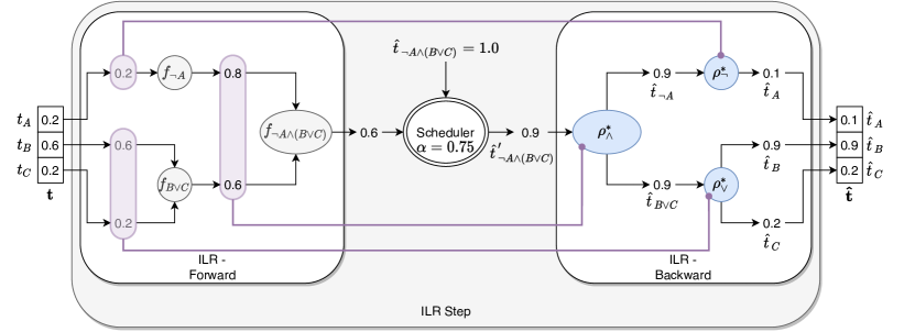
Figure 2: Visualization of one step of ILR for the Gödel logic and formula $\phi=\lnot A\land(B\lor C)$. In the forward pass (left), ILR computes the truth value of $\phi$. In the backward pass (right), ILR traverses the computational graph of the forward step in reverse to calculate the refined vector ${\hat{{\bm{t}}}}$. ILR substitutes each fuzzy operator of the forward pass with the corresponding refinement function. Each refinement function receives as input the initial truth values used by the fuzzy operator in the forward step (purple lines) and the target value for the corresponding subformula. The scheduler calculates the target value $\hat{t}^{\prime}_{\lnot A\land(B\lor C)}$ for the entire formula, which ILR calls between the forward and backward steps.

We introduce a fast, iterative, differentiable but approximate algorithm called Iterative Local Refinement (ILR) that finds minimal refinement functions for general formulas. ILR is a forward-backward algorithm acting on the computation graph of formulas. First, it traverses the graph from its leaves to its root to compute the current truth values of subformulas. Then, it traverses the graph back from its root to the leaves to compute new truth values for the subformulas. ILR makes use of analytical minimal refinement functions to perform this backward pass. ILR is a differentiable algorithm if the fuzzy operators and their corresponding minimal refinement functions are differentiable as it computes compositions of these functions. An example of one step of the ILR algorithm is presented in Figure 2, while Algorithm 1 contains the entire pseudocode.

First, ILR computes the truth value of the formula in the forward pass (left side of Figure 2), where the truth vectors of intermediate subformulas are saved (in Algorithm 1: ${\bm{t}}_{\mathsf{sub}}$. In Figure 2: numbers inside colored boxes). Then, ILR computes a backward pass (right side of Figure 2). ILR uses previously computed truth vectors of subformulas to compute the minimal refined vectors for the components of that subformula. We use the results from Sections 7.2 to compute these for the Gödel, Łukasiewicz and product fuzzy operators.

In lines 14 to 20, ILR computes the minimal refined vector for a conjunction of subformulas. We retrieve the truth values of the subformulas from the forward pass and call the minimal refinement function $\rho^{*}_{T}$ for the chosen t-norm. This procedure gives us a refined vector, where each value corresponds to the refined value of a subformula. ILR then goes in recursion on the subformulas. Note that the pseudocode for disjunction and implication is analogous.

One choice in ILR is how to combine the results from different subformulas. When a proposition appears in multiple subformulas, it can be assigned multiple different refined values. We found the heuristic in line 19 generally works well, which takes the ${\hat{t}}_{j}$ with the largest absolute value. We also explored averaging the different refined values, but this took significantly longer to converge. Another choice is the convergence criterion. A simple option is to stop running the algorithm whenever it has stopped getting closer to the refined value for a couple of iterations. In our experiments, we observed that ILR monotonically decreases the distance to the refined value, after which it gets stuck either on a single local optimum or oscillates between two local minima.

Moreover, we experimented with a scheduling mechanism to smooth the behavior of ILR. We implement this in line 7. The scheduling mechanism works by choosing a different refined value at each iteration: The difference between the current truth value and the refined value is multiplied by a scheduling parameter $\alpha$, which we choose to be either 0.1 or 1 (no scheduling). While usually not necessary, for some formulas, the scheduling mechanism allowed for finding better solutions.

ILR is not guaranteed to find a refined vector ${\hat{{\bm{t}}}}$ such that $f_{\varphi}({\hat{{\bm{t}}}})={\hat{t}_{\varphi}}$. This is easy to see theoretically because, for many fuzzy logics like the product and Gödel logics, ${\hat{t}_{\varphi}}=1$ corresponds to the PMaxSAT problem, which is NP-complete Diligenti et al. (2017); Giunchiglia et al. (2022a), while ILR has linear time complexity. However, this is traded off by 1) being highly efficient, usually requiring only a couple of iterations for convergence, and 2) not having any hyperparameters to tune, except arguably for the combination function. Furthermore, ILR usually converges quickly in neuro-symbolic settings since background knowledge is very structured, and the solution space is relatively dense. These settings are unlike the randomly generated SAT problems we study in Section 9.1.3. These contain little structure the ILR algorithm can exploit.

Algorithm 1 Iterative Local Refinement

1:$\varphi,{\hat{t}_{\varphi}},{\bm{t}}$, $\alpha\in(0,1]$

2:${\bm{t}}^{\prime}\leftarrow{\bm{t}}$

3:while not converged do

4:     ${\bm{t}}_{\mathsf{sub}}\leftarrow\{\}$

5:     for subformula $\phi$ of $\varphi$ do

6:         ${\bm{t}}_{\mathsf{sub}}[\phi]\leftarrow f_{\phi}({\bm{t}}^{\prime})$ $\ignorespaces\triangleright$ Forward pass using Definition 4      

7:     ${\hat{t}_{\varphi}}^{\prime}\leftarrow f_{\varphi}({\bm{t}})+({\hat{t}_{\varphi}}-f_{\varphi}({\bm{t}}))\alpha$

8:     ${\bm{t}}^{\prime}\leftarrow$ Backward($\varphi$, ${\hat{t}_{\varphi}}^{\prime}$, ${\bm{t}}_{\mathsf{sub}}$)

9:return ${\bm{t}}^{\prime}$

10:function Backward($P_{i}$, ${\hat{t}_{P_{i}}}$, ${\bm{t}}_{\mathsf{sub}}$)

11:     return $[t_{1},\dots,{\hat{t}_{P_{i}}},\dots,t_{n}]^{\top}$ $\ignorespaces\triangleright$ ${\bm{t}}$ except at position $i$.

12:function Backward($\neg\phi$, ${\hat{t}_{\neg\phi}}$, ${\bm{t}}_{\mathsf{sub}}$)

13:     return Backward($\phi$, $1-{\hat{t}_{\neg\phi}}$, ${\bm{t}}_{\mathsf{sub}}$)

14:function Backward($\bigwedge_{i=1}^{m}\phi_{i}$, ${\hat{t}_{\varphi}}$, ${\bm{t}}_{\mathsf{sub}}$)

15:     ${\hat{{\bm{t}}}}_{\wedge}\leftarrow\rho^{*}_{T}(\left[{\bm{t}}_{\mathsf{sub}}[\phi_{1}],...,{\bm{t}}_{\mathsf{sub}}[\phi_{m}]\right]^{\top},{\hat{t}_{\varphi}})$ $\ignorespaces\triangleright$ Minimal refinement function

16:     ${\hat{{\bm{t}}}}\leftarrow\bm{0}$

17:     for $i\leftarrow 1$ to $m$ do

18:         ${\hat{{\bm{t}}}}^{\prime}\leftarrow$ Backward($\phi_{i}$, ${\hat{t}}_{\wedge,i}$, ${\bm{t}}_{\mathsf{sub}}$)

19:         ${\hat{t}}_{j}\leftarrow$ if $|{\hat{t}}_{j}|>|{\hat{t}}^{\prime}_{j}|$ then ${\hat{t}}_{j}$ else ${\hat{t}}^{\prime}_{j}$ for all $j\in\{1,...,n\}$      

20:     return ${\hat{{\bm{t}}}}$

6 Neuro-Symbolic AI using ILR

The ILR algorithm can be added as a module after a neural network $g$ to create a neuro-symbolic AI model. The neural network predicts (possibly some of) the initial truth values ${\bm{t}}$. Since both the forward and backward passes of ILR are differentiable computations, we can treat ILR as a constrained output layer Giunchiglia et al. (2022b). For instance, in Figure 2, the input ${\bm{t}}$ could be generated by the neural network, and we provide supervision directly on the predictions ${\hat{{\bm{t}}}}$. ILR ensures the predictions, i.e., the refined vector ${\hat{{\bm{t}}}}$, satisfy the background knowledge while staying close to the original predictions made by the neural network. Loss functions like cross-entropy can use ${\hat{{\bm{t}}}}$ as the prediction. We train the neural network $g$ by minimizing the loss function with gradient descent and backpropagating through the ILR layer.

One strength of ILR is the flexibility of the refinement values ${\hat{t}_{\varphi_{i}}}$ for each formula $\varphi_{i}$. These can be set to 1 to treat $\varphi_{i}$ as a hard constraint that always needs to be satisfied. Alternatively, refinement values can be trained as part of a larger deep learning model. Since ILR is a differentiable layer, we can compute gradients of the refinement values. This procedure allows ILR to learn what formulas are useful for prediction. For instance, in Figure 2, ${\hat{t}_{\lnot A\land(B\lor C)}}$ can either be given or act as a parameter of the model that is learned together with the neural network parameters.

We give an example of the integration of ILR with a neural network in Figure 3, where we use ILR for the MNIST Addition task proposed by Manhaeve et al. (2018). In this task, we have access to a training set composed of triplets $(x,y,z)$, where $x$ and $y$ are images of MNIST LeCun and Cortes (2010) handwritten digits, and $z$ is a label representing an integer in the range $\{0,...,18\}$, corresponding to the sum of the digits represented by $x$ and $y$. The task consists of learning the addition function and a classifier for the MNIST digits, with supervision only on the sums. To achieve this, knowledge consisting of the rules of addition is given. For instance, the rule $Is(x,3)\land Is(y,2)\to Is(x+y,5)$ states that the sum of 3 and 2 is 5.

The architecture of Figure 3 consists of a neural network (a CNN) that performs digit recognition on the inputs $x$ and $y$. After this step, ILR predicts a truth value for each possible sum. Notice that we define the CNN outputs $\bm{C}_{x},\bm{C}_{y}\in[0,1]^{10}$ as constants, i.e., ILR does not change the predictions of the digits. Moreover, the initial prediction for the truth vector of possible sums ${\bm{t}}_{x+y}\in[0,1]^{19}$ is the zero vector. This allows ILR to act as a proof-based method. Indeed, similarly to DeepProbLog Manhaeve et al. (2018), the architecture proposed in Figure 3 uses the knowledge in combination with the predictions of the neural network to derive truth values for new statements (the sum of the two digits). We apply the loss function to the final predictions $\hat{{\bm{t}}}_{x+y}$. During learning, the error is back-propagated through the entire model, reaching the CNN, which learns to classify the MNIST images from indirect supervision.

We present the results obtained by ILR in Section 9.2, and compare its performance with other neuro-symbolic AI frameworks.

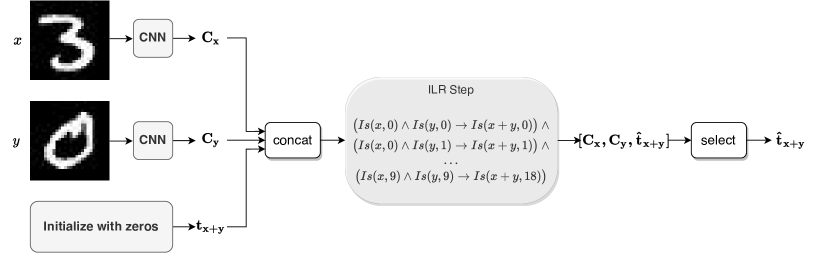
Figure 3: Neuro-symbolic architecture based on ILR for the MNIST Addition task. A CNN takes in input two images of MNIST digits, returning their classification. The predictions of the CNN are concatenated together with a vector of zeros, representing the initial prediction for the Addition task. We perform an ILR step to update the sum of the two numbers, which is the final output of the model.

7 Analytical minimal refinement functions

Having introduced the ILR algorithm, we next study the problem of finding minimal refinement functions for individual fuzzy operators. We need these in closed form to compute the ILR algorithm, as ILR uses them during the backward pass. This section first discusses several transformations of minimal refinement functions and gives the minimal refinement functions of the basic t-norms Gödel, Łukasiewicz  and product. In Section 7 we investigate a large class of t-norms for which we have closed-form formulas for the minimal refinement functions.

7.1 General results

We first provide several basic results on minimal refinement functions for fuzzy operators. In particular, we will consider formulas such as $\varphi=\bigwedge_{i=1}^{n}P_{i}\bigwedge_{i=1}^{m}C_{i}$, that is, conjunctions of propositions and constants. As abuse of notation, from here on, we will refer to ${\min_{\varphi}}$ and ${\max_{\varphi}}$ when evaluated by the t-norm $T$ as ${\min_{T}}$ and ${\max_{T}}$ and will do so also for other fuzzy operators. We find using Definition 1 that for some t-norm $T$, ${\min_{T}}=0$ and ${\max_{T}}=T({\bm{c}})$, where ${\bm{c}}$ is the values of the constants $C_{1},...,C_{m}$ as a truth vector, while for some t-conorm $S$, ${\min_{S}}=S({\bm{c}})$ and ${\max_{S}}=1$. Note that for $m=0$, ${\max_{T}}=1$ and ${\min_{S}}=0$. Next, we find some useful transformations of minimal refinement functions to derive new results:

Proposition 1.

Consider the formulas $\phi=\bigwedge_{i=1}^{n}P_{i}\bigwedge_{i=1}^{m}C_{i}$ and $\psi=\neg(\bigvee_{i=1}^{n}P_{i}\bigvee_{i=1}^{m}C_{i})$. Assume $\rho^{*}_{\phi}$ is a minimal refinement function for $f_{\phi}$ evaluated using t-norm $T$. Consider $f_{\psi}({\bm{t}})$ evaluated using dual t-conorm $S$ of $T$. Then $\rho^{*}_{\psi}({\bm{t}},{\hat{t}_{\psi}})=\bm{1}-\rho^{*}_{\phi}(\bm{1}-{\bm{t}},{\hat{t}_{\psi}})$ is a minimal refinement function for $f_{\psi}$.

Proof: First, note $f_{\psi}({\bm{t}})=1-S({\bm{t}},{\bm{c}})=1-(1-T(\bm{1}-{\bm{t}},\bm{1}-{\bm{c}}))=T(\bm{1}-{\bm{t}},\bm{1}-{\bm{c}})$. Consider ${\bm{t}}^{\prime}=\bm{1}-{\bm{t}}$. By the assumption of the proposition, $\rho^{*}_{\phi}({\bm{t}}^{\prime},{\hat{t}_{\phi}})$ is a minimal refinement function for $T({\bm{t}}^{\prime},\bm{1}-{\bm{c}})=T(\bm{1}-{\bm{t}},\bm{1}-{\bm{c}})=f_{\psi}({\bm{t}})$. Furthermore, note that

$$f_{\psi}(\rho^{*}_{\psi}({\bm{t}},{\hat{t}_{\psi}}))=T(\bm{1}-\rho^{*}_{\psi}({\bm{t}},{\hat{t}_{\psi}}),\bm{1}-{\bm{c}})=T(\rho^{*}_{\phi}({\bm{t}}^{\prime},{\hat{t}_{\psi}}),\bm{1}-{\bm{c}})={\hat{t}_{\psi}}$$

An analogous argument can be made for $\phi^{\prime}=\bigvee_{i=1}^{n}P_{i}\bigvee_{i=1}^{m}C_{i}$ and $\psi=\neg(\bigwedge_{i=1}^{n}P_{i}\bigwedge_{i=1}^{m}C_{i})$ to show that, given minimal refinement function $\rho^{*}_{\phi^{\prime}}$ of dual t-conorm $S$, the minimal refinement function for $f_{\psi}({\bm{t}})$ is $\rho^{*}_{\psi}({\bm{t}},{\hat{t}_{\psi}})=\bm{1}-\rho^{*}_{\phi}(\bm{1}-{\bm{t}},{\hat{t}_{\psi}})$.

We will use this result to simplify the process of finding minimal refinement functions for the t-norms and dual t-conorms. For example, assume we have a minimal refinement function $\rho^{*}_{T}$ for ${\hat{t}_{T}}\in[T({\bm{t}}),{\max_{T}}]$. Let $S$ be the corresponding dual t-conorm. Then, we can change the constraint $S({\hat{{\bm{t}}}},{\bm{c}})={\hat{t}_{S}}$ in Equation 7 to the equivalent constraint $\bm{1}-S({\hat{{\bm{t}}}},{\bm{c}})=\bm{1}-{\hat{t}_{S}}$. We then use Proposition 1 to find the minimal refined vector for ${\hat{t}_{S}}\in[{\min_{S}},S({\bm{t}})]$ as $\bm{1}-\rho^{*}_{T}(\bm{1}-{\bm{t}},1-{\hat{t}_{S}})$.

Proposition 2.

Consider the formulas $\phi=P_{1}\vee P_{2}$ and $\psi=\neg P_{1}\vee P_{2}$. Assume $\rho^{*}_{\phi}$ is a minimal refinement function for $f_{\phi}$ evaluated using the t-conorm $S$, and define ${\bm{t}}^{\prime}=[1-t_{1},t_{2}]$. Then $\rho^{*}_{\psi}({\bm{t}},{\hat{t}_{\psi}})=\left[1-\rho^{*}_{\phi}({\bm{t}}^{\prime},{\hat{t}_{\psi}})_{1},\rho^{*}_{\phi}({\bm{t}}^{\prime},{\hat{t}_{\psi}})_{2}\right]^{\top}$ is a minimal refinement function for $f_{\psi}$.

Proof: First, note $f_{\psi}({\bm{t}})=S(1-{\bm{t}}_{1},{\bm{t}}_{2})$. By the assumption of the proposition, $\rho^{*}_{\phi}({\bm{t}}^{\prime},{\hat{t}_{\psi}})$ is a minimal refinement function for $S({\bm{t}}^{\prime})=f_{\psi}({\bm{t}})$. Furthermore, note that

$$f_{\psi}(\rho^{*}_{\psi}({\bm{t}},{\hat{t}_{\psi}})) =S(1-\rho^{*}_{\psi}({\bm{t}}^{\prime},{\hat{t}_{\psi}})_{1},\rho^{*}_{\psi}({\bm{t}}^{\prime},{\hat{t}_{\psi}})_{2})$$

$$=S(1-(1-\rho^{*}_{\phi}({\bm{t}}^{\prime},{\hat{t}_{\psi}})_{1}),\rho^{*}_{\phi}({\bm{t}}^{\prime},{\hat{t}_{\psi}})_{2})=S(\rho^{*}_{\phi}({\bm{t}}^{\prime},{\hat{t}_{\psi}}))={\hat{t}_{\psi}}.$$

Similar to the previous proposition, this proposition gives us a simple procedure for finding the minimal refinement functions for the S-implication of some t-conorm.

7.2 Basic T-norms

In this section, we introduce the minimal refinement functions for the t-norms and t-conorms of the three main fuzzy logics (Gödel, Łukasiewicz, and Product). In particular, we consider when these t-norms and t-conorms can act on both propositions and constants, that is, $\varphi=\bigwedge_{i=1}^{n}t_{i}\bigwedge_{i=1}^{m}C_{i}$, which is evaluated with $T({\bm{t}},{\bm{c}})$. We present the main results with simple examples.

7.2.1 Gödel t-norm

In this section, we derive minimal refinement functions for the Gödel t-norm and t-conorm for the family of $p$-norms.

Proposition 3.

The minimal refinement function of the Gödel t-norm for ${\hat{t}_{T_{G}}}\in[0,\min_{i=1}^{m}C_{i}]$ is

$$\rho^{*}_{T_{G}}({\bm{t}},{\hat{t}_{T_{G}}})_{i}=\begin{cases}{\hat{t}_{T_{G}}}&\text{if }{\hat{t}_{T_{G}}}\geq T_{G}({\bm{t}})\text{ and }t_{i}<{\hat{t}_{T_{G}}},\\ {\hat{t}_{T_{G}}}&\text{if }{\hat{t}_{T_{G}}}<T_{G}({\bm{t}})\text{ and }i=\arg\min_{j=1}^{n}t_{j},\\ t_{i}&\text{otherwise,}\end{cases}$$ (8)

The minimal refinement function of the Gödel t-conorm and ${\hat{t}_{S_{G}}}\in[\max_{i=1}^{m}C_{i},1]$ is

$$\rho^{*}_{S_{G}}({\bm{t}},{\hat{t}_{S_{G}}})_{i}=\begin{cases}{\hat{t}_{S_{G}}}&\text{if }{\hat{t}_{S_{G}}}\geq S_{G}({\bm{t}})\text{ and }i=\arg\max_{j=1}^{m}t_{j},\\ {\hat{t}_{S_{G}}}&\text{if }{\hat{t}_{S_{G}}}<S_{G}({\bm{t}})\text{ and }t_{i}>{\hat{t}_{S_{G}}},\\ 0&\text{otherwise.}\end{cases}$$ (9)

Proof: Follows from Propositions 1, 10 and 11, see Appendix A.1.1 and A.1.2.

Proposition 4.

A minimal refinement function of the Gödel implication $R_{G}(t_{1},t_{2})=\begin{cases}t_{2}&\text{if }t_{1}>t_{2},\\ 1&\text{otherwise.}\end{cases}$ for ${\hat{t}_{R_{G}}}\in[{\min_{R_{G}}},{\max_{R_{G}}}]$ is

$$\rho^{*}_{R_{G}}(t_{1},t_{2},{\hat{t}_{R_{G}}})=\begin{cases}[\max({\hat{t}_{R_{G}}}+\epsilon,t_{1}),{\hat{t}_{R_{G}}}]^{\top}&\text{if }{\hat{t}_{R_{G}}}<1\\ [t_{1},\max(t_{1},t_{2})]^{\top}&\text{otherwise.}\end{cases}$$ (10)

where $\epsilon$ is an arbitrarily small positive number.

The proof is in Appendix 4.

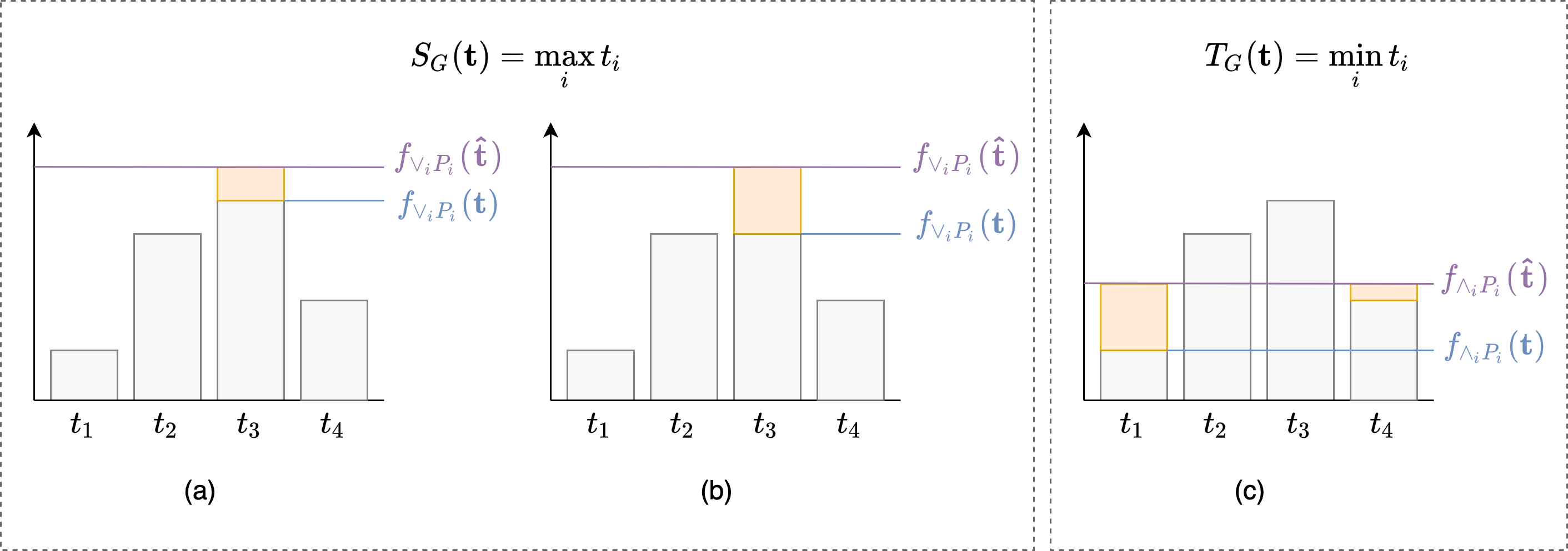
Figure 4: Gödel minimal refinement functions. The grey bars represent the initial truth vectors ${\bm{t}}$; the light blue and purple lines indicate the initial truth value of the formula and the revision value ${\hat{t}_{\varphi}}$, and the orange bars are the corresponding minimal refined vectors. (a) t-conorm; (b) t-conorm with two literals with same truth value; (c) t-norm.

The bar plot in Figure 4(a) shows an example for the Gödel t-conorm with four literals. The minimal refined vector is represented with the orange boxes, while the initial and refinement values of the entire formula are represented as a blue and purple line respectively. Here, our goal is to increase the value of the t-conorm, i.e., the maximum value. Increasing other literals up to ${\hat{t}_{\varphi}}$ would require longer orange bars and bigger values for the L_p norm. Figure 4(b) represents when multiple literals have the largest truth value. Here, only one should be increased. Finally, Figure 4(c) shows the refined vector for the Gödel t-norm. Since the smallest truth value should be at least ${\hat{t}_{\varphi}}$, we simply ensure all truth values are at least ${\hat{t}_{\varphi}}$.

Our results are closely related to that of Giunchiglia and Lukasiewicz (2021), which considers hard constraints, i.e., ${\hat{t}_{\varphi}}=1$. In the hierarchical multi-label classification setting, the authors introduce an output layer that ensures predictions satisfy a set of hierarchy constraints. This layer corresponds to applications of the minimal refinement function for the Gödel implication with ${\hat{t}_{R_{G}}}=1$. Furthermore, Giunchiglia and Lukasiewicz (2021) introduces C-HMCNN(h). This method considers an output layer that ensures predictions satisfy background knowledge expressed in a stratified normal logic program. The authors introduce an iterative algorithm that computes the minimal solution for such programs. This algorithm is related to that of ILR in Section 5. However, their formalization differs somewhat from ours, and future work could study whether these results also hold for our formalization of minimal refinement functions and if they can be extended to any value of ${\hat{t}_{\varphi}}$. Finally, Giunchiglia and Lukasiewicz (2021) introduces a loss function that compensates for gradient bias introduced by the constrained output layer.

7.2.2 Łukasiewicz t-norm

In this section, we derive minimal refinement functions for the Łukasiewicz t-norm and t-conorm, for the family of $p$-norms. We will start using the following notation here: ${\bm{t}}^{\uparrow}$ refers to the truth values $t_{i}$ sorted in ascending order, while ${\bm{t}}^{\downarrow}$ refers to the truth values sorted in descending order.

Proposition 5.

Let ${\hat{t}_{T_{L}}}\in[0,\max(\|{\bm{c}}\|_{1}-(m-1),0)]$ and define $\lambda_{K}=\frac{{\hat{t}_{T_{L}}}+m+K-1-\|{\bm{c}}\|_{1}-\sum_{i=1}^{K}t^{\uparrow}_{i}}{K}$. Let $K^{*}$ be the largest integer $1\leq K\leq n$ such that $\lambda_{K}<1-t^{\uparrow}_{K}$. Then the minimal refinement vector of the Łukasiewicz t-norm is

$$\rho^{*}_{T_{L}}({\bm{t}},{\hat{t}_{T_{L}}})_{i}=\begin{cases}t_{i}+\lambda_{K^{*}}&\text{if }{\hat{t}_{T_{L}}}>T_{L}({\bm{t}})\text{ and }t_{i}\leq t^{\uparrow}_{K^{*}},\\ 1&\text{if }{\hat{t}_{T_{L}}}>T_{L}({\bm{t}})\text{ and }t_{i}>t^{\uparrow}_{K^{*}},\\ t_{i}-\frac{\max(\|{\bm{t}}\|_{1}+\|{\bm{c}}\|_{1}+1-n-{\hat{t}_{T_{L}}},0)}{n}&\text{otherwise.}\end{cases}$$ (11)

Let ${\hat{t}_{S_{L}}}\in[\min(\|{\bm{c}}\|_{1},1),1]$ and define $\lambda_{K}=\frac{\|{\bm{t}}\|_{1}+\|{\bm{c}}\|_{1}-{\hat{t}_{S_{L}}}}{K}$. Let $K^{*}$ be the largest integer $1\leq K\leq n$ such that $\lambda_{K}<t^{\downarrow}_{K}$. Then the minimal refinement function of the Łukasiewicz t-conorm is

$$\rho^{*}_{S_{L}}({\bm{t}},{\hat{t}_{S_{L}}})_{i}=\begin{cases}t_{i}+\frac{\max({\hat{t}_{S_{L}}}-\|{\bm{t}}\|_{1}-\|{\bm{c}}\|_{1},0)}{n}&\text{if }{\hat{t}_{S_{L}}}>S_{L}({\bm{t}}),\\ t_{i}-\lambda_{K^{*}}&\text{if }{\hat{t}_{S_{L}}}<S_{L}({\bm{t}})\text{ and }t_{i}\geq t^{\downarrow}_{K^{*}},\\ 0&\text{otherwise.}\end{cases}$$ (12)

Proof: This follows from Propositions 1, 12 and 13, see Appendix A.2.1 and A.2.2.

Although slightly obfuscated, these refinement functions simply increase each of the literals equally, while properly dealing with constraints on the truth values. We explain this using Figure 5, where the optimal solution corresponds to a vector that, from the original truth values ${\bm{t}}$, is perpendicular to the contour line of the operator at the value ${\hat{t}_{\varphi}}$. Moreover, the figure also provides some intuition for our proofs. The stationary points of the Lagrangian correspond to the points where the constraint function (blue circumference) tangentially touches the contour line of the refined value (orange line).

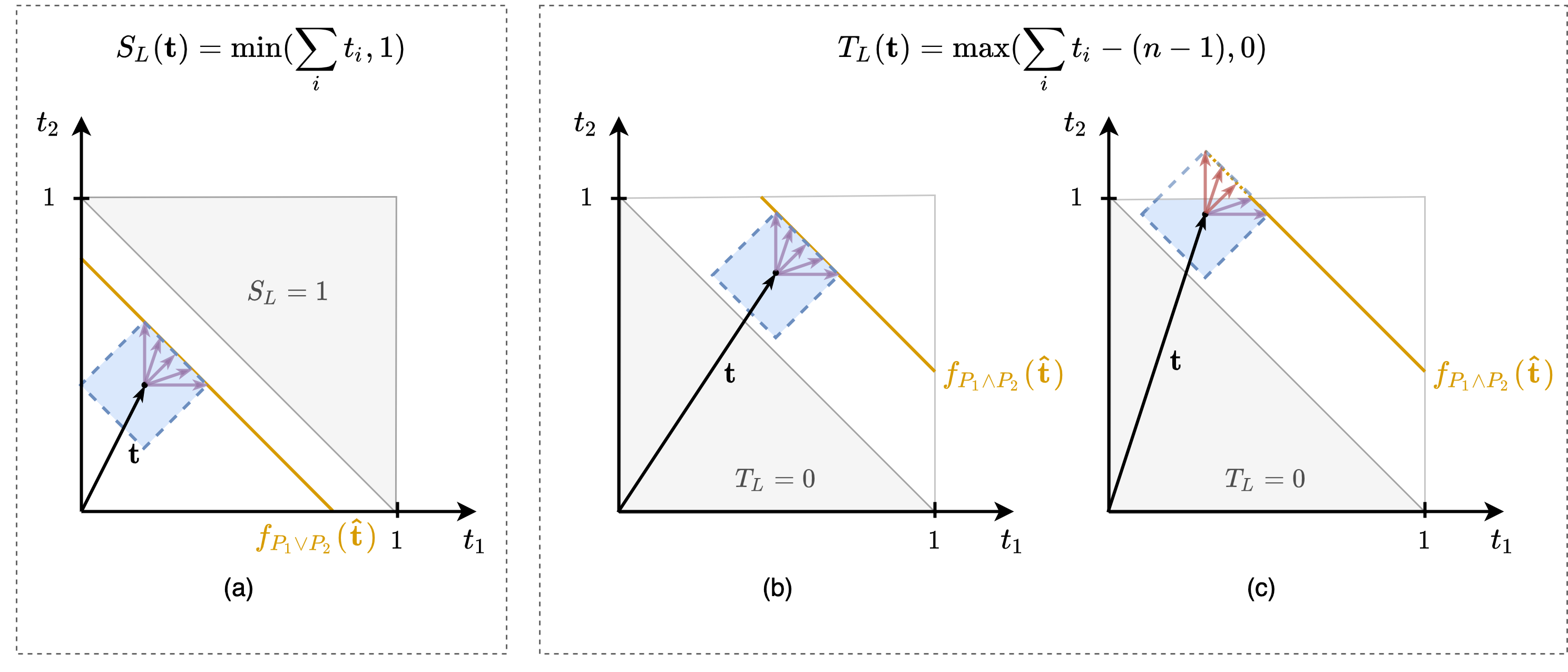
Figure 5: Łukasiewicz minimal refinement functions. The orange line corresponds to the contour line of the $S_{L}$ and $T_{L}$ at the value ${\hat{t}_{\varphi}}$. Dotted blue circumference corresponds to a set of points at an equal distance from ${\bm{t}}$. (a) t-conorm; (b) t-norm; (c) t-norm in the limit case.

The change applied by the refinement function is proportional to the refinement value ${\hat{t}}$. Computing these refinement functions requires finding $K^{*}$, which can be done efficiently in log-linear time using a sort on the input truth values and a binary search.

The residuum of the Łukasiewicz t-norm is equal to its S-implication formed using $S_{L}(1-a,c)$, and so its minimal refinement function can be found using Proposition 2.

The Łukasiewicz logic is unique in containing large convex and concave fragments Giannini et al. (2019). In particular, any CNF formula interpreted using the weak conjunction (Godel t-norm) and Łukasiewicz t-conorm is concave, allowing for efficient maximization using a quadratic program of a slightly relaxed variant of the problem in Equation 7. Giannini et al. (2019) studies this property in a setting similar to ours in the context of collective classification. Future work could study using this convex fragment to find minimal refinement functions for more complex formulas.

7.2.3 Product t-norm

To present the three basic t-norms together, we give the closed-form refinement function for the product t-norm with the L1 norm. Our proof is a special case of the general results on a large class of t-norms we will discuss in Section 7. In particular, the product t-norm is a strict, Schur-concave t-norm with an additive generator. It is an example of a t-norm for which we can find a closed-form refinement function for the L1 norm using Propositions 15 and 1. First, we show the minimal refinement function for the product t-norm.

$$\rho^{*}_{T_{P}}({\bm{t}},{\hat{t}_{T_{P}}})_{i}=\begin{cases}\sqrt[n-K^{*}]{\frac{{\hat{t}_{T_{P}}}}{\prod_{j=1}^{K^{*}}t_{j}^{\downarrow}\prod_{j=1}^{m}C_{j}}}&\text{if }T_{P}({\bm{t}},{\bm{c}})>{\hat{t}_{T_{P}}}\text{ and }t_{i}\leq t^{\downarrow}_{K^{*}+1},\\ \sqrt{\frac{{\hat{t}_{T_{P}}}}{\prod_{j\neq i}t_{i}^{\downarrow}\prod_{i=1}^{m}C_{i}}}&\text{if }T_{P}({\bm{t}},{\bm{c}})<{\hat{t}_{T_{P}}}\text{ and }i=\arg\min_{j=1}^{n}t_{j},\\ t_{i}&\text{otherwise.}\end{cases}$$ (13)

Next, we present the result for the product t-conorm:

$$\rho^{*}_{S_{P}}({\bm{t}},{\hat{t}_{S_{P}}})_{i}=\begin{cases}1-\sqrt{\frac{1-{\hat{t}_{S_{P}}}}{\prod_{j\neq i}1-t_{i}^{\downarrow}\prod_{i=1}^{m}1-C_{i}}}&\text{if }S_{P}({\bm{t}},{\bm{c}})<{\hat{t}_{S_{P}}}\text{ and }i=\arg\min_{j=1}^{n}t_{j},\\ 1-\sqrt[n-K^{*}]{\frac{1-{\hat{t}_{S_{P}}}}{\prod_{j=1}^{K^{*}}1-t_{j}^{\downarrow}\prod_{j=1}^{m}1-C_{j}}}&\text{if }S_{P}({\bm{t}},{\bm{c}})>{\hat{t}_{S_{P}}}\text{ and }t_{i}\leq t^{\downarrow}_{K^{*}+1},\\ t_{i}&\text{otherwise.}\end{cases}$$ (14)

This refined function increases all the literals smaller than a certain threshold up to the threshold itself, where we assume ${\hat{t}_{T_{P}}}$ is greater than the initial truth value. In fact, like the other t-norms in the class discussed in Section 7, it is similar to the Gödel t-norm in that it increases all literals above some threshold to the same value. Similarly, the refinement function for the t-conorm increases the highest literal. Figure 6 gives an intuition behind this behaviour.

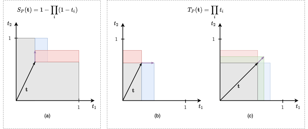
Figure 6: Product minimal refinement functions. The grey areas represent the truth value of the operator associated with the initial vector ${\bm{t}}$. Red and blue areas represent the refined values when increasing a single literal. (a) t-conorm; (b) t-norm; (c) t-norm when multiple literals have same truth value. The green area represents the improvement obtained by increasing both literals equally.

Finally, the residuum minimal refinement function can be found with $\rho^{*}_{I_{P}}(t_{1},t_{2},{\hat{t}_{I_{P}}})=[t_{1},\frac{{\hat{t}_{I_{P}}}}{t_{1}}]^{\top}$.

We also studied the minimal refinement function for the L2 norm, but concluded that the result is a $2n$th degree polynomial with no simple closed-form solutions. For details, see Appendix D.

8 A general class of t-norms with analytical minimal refinement functions

In this section, we will introduce and discuss a general class of t-norms that have analytic solutions to the problem in Equation 7 in order to find their corresponding minimal refinement functions. We can find those for the t-norm, t-conorm, and the residuum.

8.1 Background on t-norms

To be able to properly discuss this class of t-norms, we first have to provide some more background on the theory of t-norms.

8.1.1 Additive generators

The study of t-norms frequently involves the study of their additive generator Klement et al. (2013, 2004), which are univariate functions that can be used to construct t-norms, t-conorms and residuums.

Definition 7.

A function $g:[0,1]\rightarrow[0,\infty]$ such that $g(1)=0$ is an additive generator if it is strictly decreasing, right-continuous at 0, and if for all $t_{1},t_{2}\in[0,1]$, $g(t_{1})+g(t_{2})$ is either in the range of $g$ or in $[g(0^{+}),\infty]$.

Theorem 1.

If $g$ is an additive generator, then the function $T:[0,1]^{n}\rightarrow[0,1]$ defined as

$$T({\bm{t}})=g^{-1}(\min(g(0^{+}),\sum_{i=1}^{n}g(t_{i})))$$ (15)

is a t-norm.

Using Equation 15, the function $g$ acts like an invertible function. It transforms truth values into a new space that can be seen as measuring ‘untruthfulness’. $\sum_{i=1}^{n}g(t_{i})$ can be seen as a measure of ‘untruth’ of the conjunction. T-norms constructed in this way are necessarily Archimedean, and each continuous Archimedean t-norm has an additive generator. $T_{P}$, $T_{L}$ and $T_{D}$ have an additive generator, but $T_{G}$ and $T_{N}$ do not. Furthermore, if $g(0^{+})=\infty$, $T$ is strict and we find $T({\bm{t}})=g^{-1}(\sum_{i=1}^{n}g(t_{i}))$. The residuum constructed from continuous t-norms with an additive generator can be computed using $g^{-1}(\max(g(c)-g(a),0))$ Jayaram and Baczynski (2008).

8.1.2 Schur-concave t-norms

We will frequently consider the class of Schur-concave t-norms, with their dual t-conorms and residuums formed from these Schur-concave t-norms. We denote with ${\bm{t}}^{\downarrow}$ the truth vector ${\bm{t}}$ sorted in descending order, and with ${\bm{t}}^{\uparrow}$ as ${\bm{t}}$ sorted in ascending order.

Definition 8.

A vector ${\bm{t}}\in\mathbb{R}^{n}$ is said to majorize another vector ${\bm{u}}\in\mathbb{R}^{n}$, denoted ${\bm{t}}\succ{\bm{u}}$, if $\sum_{i=1}^{n}t_{i}=\sum_{i=1}^{n}{u_{i}}$ and if for each $i\in\{1,...,n\}$ it holds that $\sum_{j=1}^{i}t_{j}^{\downarrow}\geq\sum_{j=1}^{i}u_{j}^{\downarrow}$.

Definition 9.

A function $[0,1]^{n}\rightarrow[0,1]$ is called Schur-convex if for all ${\bm{t}},{\bm{u}}\in[0,1]^{n}$, ${\bm{t}}\succ{\bm{u}}$ implies that $f({\bm{t}})\geq f({\bm{u}})$. Similarly, a Schur-concave function has that ${\bm{t}}\succ{\bm{u}}$ implies that $f({\bm{t}})\leq f({\bm{u}})$.

The dual t-conorm of a Schur-concave t-norm is Schur-convex. The three basic and continuous t-norms $T_{G}$, $T_{P}$ and $T_{L}$ are Schur-concave. There are also non-continuous Schur-concave t-norms, such as the Nilpotent minimum Takači (2005); van Krieken et al. (2022). The drastic t-norm is an example of a t-norm that is not Schur-concave Takači (2005). This class includes all quasiconcave t-norms since all symmetric quasiconcave functions are also Schur-concave (Marshall et al., 2011, p98 C.3). Therefore, this class constitutes a significant class of relevant t-norms. For a more precise characterization of Schur-concave t-norms, see Takači (2005); Alsina (1984).

8.2 Minimal refinement functions for Schur-concave t-norms

We now have the background to discuss several useful and interesting results on Schur-concave t-norms. First, we present two results that characterize Schur-concave minimal refinement functions. We use the notion of “strictly cone-increasing” functions here that is discussed in Appendix B.1.

Theorem 2.

Let $T$ be a Schur-concave t-norm that is strictly cone-increasing at ${\hat{t}_{T}}$ and let $\|\cdot\|$ be a strict norm. Then there is a minimal refined vector ${{\bm{t}}^{*}}$ for ${\bm{t}}$ and ${\hat{t}_{T}}$ such that whenever $t_{i}>t_{j}$, then ${t^{*}}_{i}-t_{i}\leq{t^{*}}_{j}-t_{j}$.

For proof, see Appendix C.1. We note that we can make this argument in the other direction to show that any Schur-convex t-conorm will have a minimal refined vector such that $t_{i}>t_{j}$ implies ${t^{*}}_{i}\geq{t^{*}}_{j}$. Furthermore, if we know that a t-norm has a unique minimal refinement function, we can use this theorem to infer a useful ordering on how it changes the truth values.

Next, we will consider the L1 norm $\sum_{i=1}^{n}|{\hat{t}}_{i}-t_{i}|$, for which we can find general solutions for the t-norm, t-conorm and R-implication when the t-norm is Schur-concave.

Proposition 6.

Let ${\bm{t}}\in[0,1]^{n}$ and let $T$ be a Schur-concave t-norm that is strictly cone-increasing at ${\hat{t}_{T}}\in[T({\bm{t}},{\bm{c}}),{\max_{T}}]$. Then there is a value $\lambda\in[0,1]$ such that the vector ${{\bm{t}}^{*}}$,

$${t^{*}}_{i}=\begin{cases}\lambda,&\text{if }t_{i}<\lambda,\\ t_{i},&\text{otherwise,}\end{cases}$$ (16)

is a minimal refined vector for $T$ and the L1 norm at ${\bm{t}}$ and ${\hat{t}_{T}}$.

For proof, see Appendix C.2. We found this result rather surprising: It is optimal for a large class of t-norms and the L1 norm to increase the lower truth values to some value $\lambda$. In this sense, these solutions are very similar to that of the Gödel refinement functions. The value of $\lambda$ depends on the choice of t-norm and $T({{\bm{t}}^{*}},{\bm{c}})$ is a non-decreasing function of $\lambda$. We show in Section 8.3 how to compute these.

We have a similar result, proof in the end of Appendix C.2, for the refinement functions of Schur-convex t-conorms. This proposition shows that, under the L1 norm, it is optimal to increase only the largest literal, just like with the Gödel t-norm.

Proposition 7.

Let ${\bm{t}}\in[0,1]^{n}$ and let $S$ be a Schur-convex t-conorm that is strictly cone-increasing at ${\hat{t}_{S}}\in[S({\bm{t}},{\bm{c}}),1]$. Then there is a value $\lambda\in[0,1]$ such that the vector ${{\bm{t}}^{*}}$,

$${t^{*}}_{i}=\begin{cases}\lambda&\text{if }i={\arg\max}_{i\in D}t_{i},\\ t_{i},&\text{otherwise,}\end{cases}$$ (17)

is a minimal refined vector for $S$ and the L1 norm at ${\bm{t}}$ and ${\hat{t}_{S}}$.

8.3 Closed forms using Additive Generators

Where the previous section gives general results on the form or “shape” of minimal refinement functions for t-norms and t-conorms under the L1 norm, we still need to figure out what the value of $\lambda$ is for a particular ${\hat{t}_{\varphi}}$. Luckily, additive generators will do the job here.

Proposition 8.

Let $T$ be a Schur-concave t-norm with additive generator $g$ and let $0<{\hat{t}_{T}}\in[T({\bm{t}},{\bm{c}}),{\max_{T}}]$. Let $K\in\{0,...,n-1\}$ denote the number of truth values such that ${t^{*}}_{i}=t_{i}$ in Equation 28. Then using

$$\lambda_{K}=g^{-1}\left(\frac{1}{n-K}\left(g({\hat{t}_{T}})-\sum_{i=1}^{K}g(t^{\downarrow}_{i})-\sum_{i=1}^{m}g(C_{i})\right)\right)$$ (18)

in Equation 28 gives $T({{\bm{t}}^{*}},{\bm{c}})={\hat{t}_{T}}$ if ${{\bm{t}}^{*}}\in[0,1]^{n}$.

See Appendix C.2 for a proof. $g({\hat{t}_{T}})$ can be seen as the ‘untruth’-value in $g$-space that ${{\bm{t}}^{*}}$ should attain. Since we have $n-K$ truth values that we can move freely, we need to make sure that their ‘untruth’-value in $g$-space is $g({\hat{t}_{T}})/(n-K)$. However, we also need to handle the truth values we cannot change freely, which is why those are subtracted from $g({\hat{t}_{T}})$.

We should note that this does not yet give a procedure for computing the correct $K\in\{0,...,n-1\}$. The intuition here is that we should find an $K$ such that $t_{i}\geq\lambda_{K}$ for the $K$ largest values, and $t_{i}<\lambda_{K}$ for the remaining $n-K$. Like with computing the $K^{*}$ for the refinement function for the Łukasiewicz t-norm (Section 7.2.2), we can do this in logarithmic time after sorting ${\bm{t}}$, but we choose to compute $\lambda_{K}$ for each $K\in\{0,n-1\}$ in parallel.

We can similarly find a closed form for the t-conorms:

$$\lambda =1-g^{-1}\left(g(1-{\hat{t}_{S}})-\sum_{i\neq j}g(1-t_{i})-\sum_{i=1}^{m}g(1-C_{i})\right)$$ (19)

Proposition 9.

Let $t_{1},t_{2}\in[0,1]$ and let $T$ be a strict Schur-concave t-norm with additive generator $g$. Consider its residuum $R(t_{1},t_{2})=\sup\{z|T(t_{1},z)\leq t_{2}\}$ that is strictly cone-increasing at $0<{\hat{t}_{R}}\in[R(t_{1},t_{2}),{\max_{R}}]$. Then there is a value $\lambda\in[0,1]$ such that ${{\bm{t}}^{*}}=[t_{1},g^{-1}(g({\hat{t}_{R}})+g(t_{1}))]^{\top}$ is a minimal refined vector for $R$ and the L1 norm at ${\bm{t}}$ and $t$.

Here, we find that for this class of residuums, increasing the consequent (the second argument of the implication) is minimal for the L1 norm. This update reflects modus ponens reasoning: When the antecedent is true, increase the consequent. As we have argued in van Krieken et al. (2022), this could cause issues in many machine learning setups: Consider the modus tollens correction instead decreases the antecedent. For common-sense knowledge, this is more likely to reflect the true state of the world.

9 Experiments

We performed experiments on two tasks. The first one does not involve learning. Instead, we aim to solve SAT problems. This experiment allows assessing whether ILR can enforce complex and unstructured knowledge. The second experiment is on the MNIST Addition task Manhaeve et al. (2018) to test ILR in a neuro-symbolic setting and assess its ability to learn from data.

9.1 Experiments on 3SAT problems

With this experiments, our goal is to find out how quickly ILR finds a refined vector and how minimal this vector is. We test this on formulas of varying complexity to analyze for what problems each algorithm performs well.

9.1.1 Setup

We perform experiments on SATLIB Hoos (2000), a library of randomly generated 3SAT problems. 3SAT problems are formulas in the form $\bigwedge_{i=1}^{c}\bigvee_{j=1}^{3}l_{ij}$, where $l_{ij}$ is a literal that is either $P_{k}$ or $\neg P_{k}$ and where $P_{k}\in\{P_{1},...,P_{n}\}$ is an input proposition. In particular, we consider uf20-91 of satisfiable 3SAT problems with $n=20$ propositions and $c=91$ disjunctive clauses. For this, we select the refined value ${\hat{t}_{\varphi}}$ to be 1. We also experiment with ${\hat{t}_{\varphi}}\in\{0.3,0.5\}$ in Appendix E. We uniformly generate initial truth values for the propositions ${\bm{t}}\in[0,1]^{d}$ . To allow experimenting with formulas of varying complexity, we introduce a simplified version of the task which uses only the first 20 clauses.

We compare ILR with a gradient descent baseline described in Section 9.1.2 using three metrics. The first is speed: How many iterations does it take for each algorithm to converge? Since both algorithms have similar computational complexities, we will use the number of iterations for this. The second is satisfaction: Is the algorithm able to find a solution with truth value ${\hat{t}_{\varphi}}$? Finally, we consider minimality: How close to the original prediction is the refined vector ${\hat{{\bm{t}}}}$? Note that the refinement function for the product logic is only optimal for the L1 norm, while for Gödel and Łukasiewicz, the refinement function is optimal for all L_p norms, including L1. Moreover, the results of L1 and L2 are very similar. Therefore, we use the L1 as a metric for minimality for each t-norm.

9.1.2 Gradient descent baseline

We compare ILR to gradient descent with the following loss function

$$\mathcal{L}(\hat{\mathbf{z}},{\bm{t}},{\hat{t}_{\varphi}})=\|f_{\varphi}(\sigma(\hat{\mathbf{z}}))-{\hat{t}_{\varphi}}\|_{2}+\alpha\|\sigma(\hat{\mathbf{z}})-{\bm{t}}\|_{p}.$$ (20)

Here ${\hat{{\bm{t}}}}=\sigma(\hat{\mathbf{z}})$ is a real-valued vector $\hat{\mathbf{z}}\in\mathbb{R}^{n}$ transformed to ${\hat{{\bm{t}}}}\in[0,1]^{n}$ using the sigmoid function $\sigma$ to ensure the values of ${\hat{{\bm{t}}}}$ remain in $[0,1]^{n}$ during gradient descent. The first term minimizes the distance between the current truth value of the formula $\varphi$ and the refinement value, while the second term is a regularization term that minimizes the distance between the refined vector and the original truth value ${\bm{t}}$ in the L$p$ norm. $\alpha$ is a hyperparameter that trades off the importance of this regularization term.

This method for finding refined vectors is very similar to the collective classification method introduced in SBR Diligenti et al. (2017); Roychowdhury et al. (2021). The main difference is in the L$p$ norms chosen, as we use squared error for the first term instead of the L1 norm. Gradient descent is a steepest descent method that take steps minimizing the L2 norm. Therefore, it can also be seen as a method for finding minimal refinement functions given the L2 norm. The corresponding steepest descent method for the L1 norm is the coordinate descent algorithm. Future work could compare how coordinate descent performs for finding minimal refinement functions for the L1 norm. We suspect it will be much slower than gradient descent-based methods as it can only change a single truth value each iteration.

We found that ADAM Kingma and Ba (2017) significantly outperformed standard gradient descent in all metrics, and we chose to use it throughout our experiments. Furthermore, inspired by the analysis of the derivatives of aggregation operators in van Krieken et al. (2022), we slightly change the formulation of the loss function for the Łukasiewicz t-norm and product t-norm. The Łukasiewicz t-norm will have precisely zero gradients for most of its domain. Therefore, we remove the $\max$ operator when evaluating the $\bigwedge$ in the SAT formula so it has nonzero gradients. For the product t-norm, the gradient will also approach 0 because of the large set of numbers between $[0,1]$ that it multplies. As suggested by van Krieken et al. (2022), we instead optimize the logarithm of the product t-norm:

$$\mathcal{L}_{P}(\hat{\mathbf{z}},{\bm{t}},{\hat{t}_{\varphi}})=\|\sum_{i=1}^{c}\log f_{\bigvee_{j=1}^{3}}(\sigma({\bm{t}}))-\log{\hat{t}_{\varphi}}\|_{2}+\alpha\|\sigma(\hat{\mathbf{z}})-{\bm{t}}\|_{1}.$$

9.1.3 Results

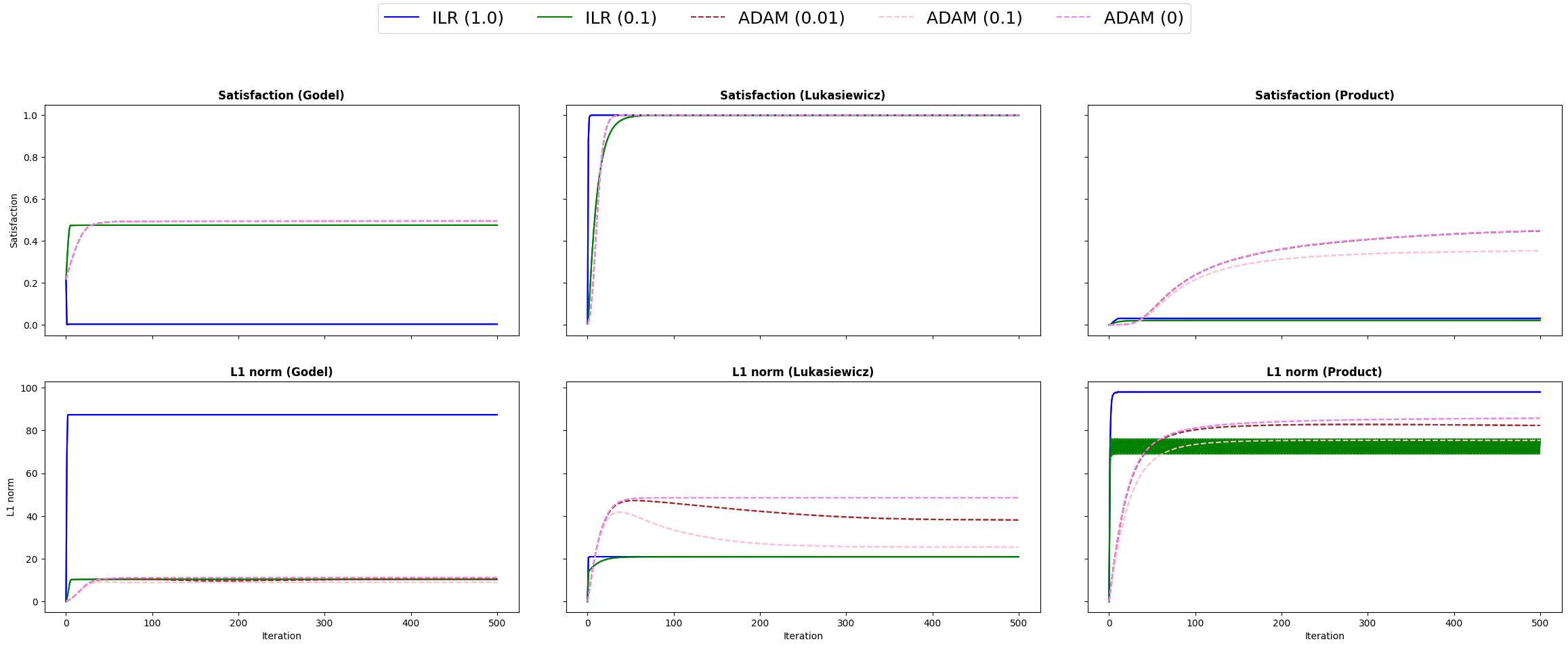
Figure 7: Comparison of ILR with ADAM on uf20-91 in SATLIB. Refined value 1.0.. The x axis corresponds to the number of iterations, while the y axis is the value of ${\hat{t}_{\varphi}}$ in the first row of the grid, and the L1 norm in the second row.

In Figure 7 we show the results obtained by ILR and ADAM on the three t-norms (one for each column of the grid). We observe that ILR with schedule parameter $\alpha=0.1$ has a smoother plot compared to ILR with $\alpha=1.0$, which converges faster: In our experiments, the number of steps until convergence was always between 2 and 5. For both values of the scheduling parameters, ILR outperforms ADAM in terms of convergence speed.

When comparing satisfaction and minimality, the behavior differs based on the t-norm used. In the case of Łukasiewicz, all methods find feasible solutions to the optimization problem. Furthermore, in terms of minimality (i.e., L1 norm), ILR finds better solutions than ADAM.

For the Gödel logic no method is capable of reaching a feasible solution. Here, ILR with schedule parameter $\alpha=1$ performs very poorly, obtaining worse solutions than the original truth values. On the other hand, with $\alpha=0.1$, it performs as well as ADAM for both metrics but with faster convergence.

Finally, for the product logic, ILR fails to increase the satisfaction of the formula to the refined value. However, ADAM can find much better solutions, getting the average truth value to around 0.5. Still, it is far from reaching a feasible solution. Nonetheless, we recommend using ADAM for complicated formulas in the product logic.

However, we argue that in the context of Neural-Symbolic Integration, the provided knowledge is usually relatively easy to satisfy. With 91 clauses, there are few satisfying solutions in this space of $2^{21}$ possible binary solutions. However, background knowledge usually does not constrain the space of possible solutions as heavily as this. For this reason, we propose a simplified formula, where we only use 20 out of 91 clauses. Figure 8 shows the results for this setting. We see that ILR with no scheduling ($\alpha=1$) finds feasible solutions for all t-norms. ILR finds solutions for the Gödel t-norm where ADAM cannot find any, while for Łukasiewicz and product, it finds solutions in much fewer iterations and with a lower L1 norm. Hence, we argue that for knowledge bases that are less constraining, ILR without scheduling is the best choice.

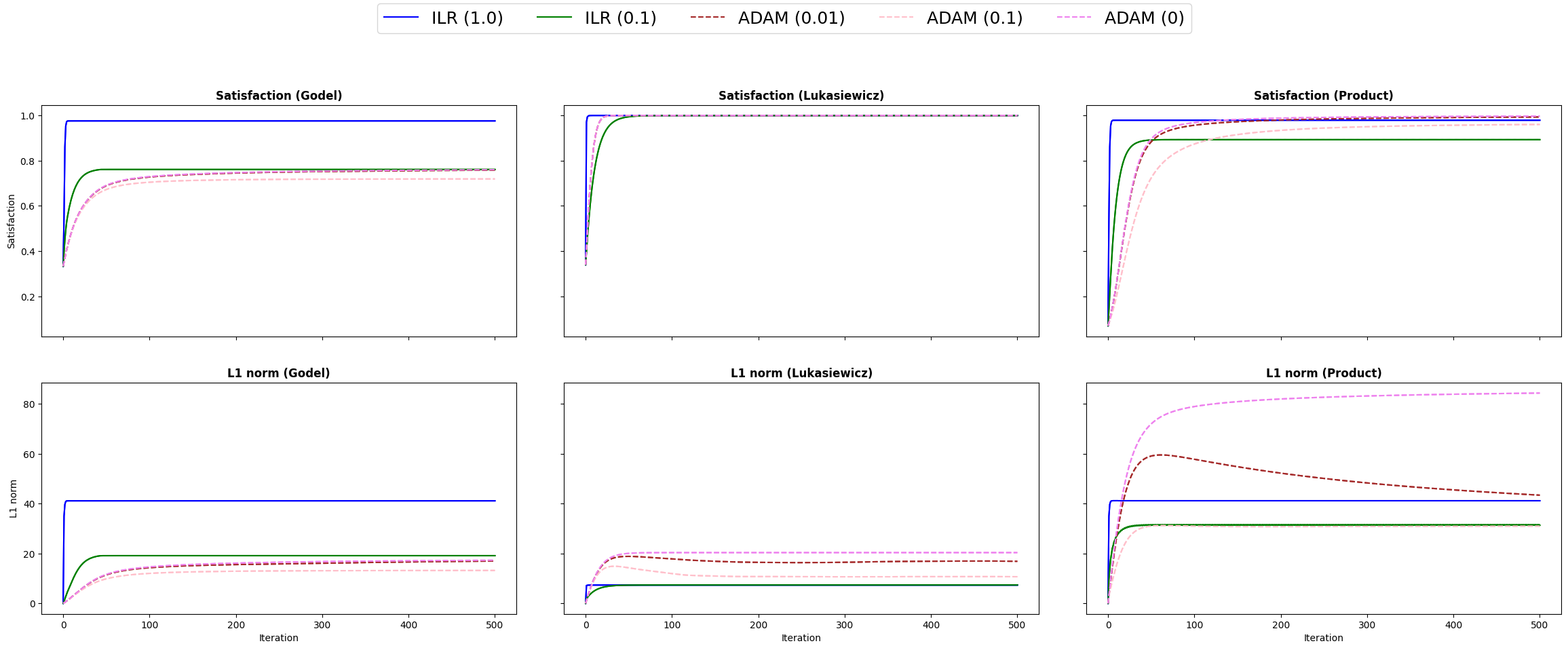
Figure 8: Comparison of ILR with ADAM on the uf20-91 with 20 clauses. Target value 1.0.

9.2 Experiments on MNIST Addition

The experiments on the SATLIB benchmark show how well ILR can enforce knowledge in highly constrained settings. However, as already mentioned, in neuro-symbolic AI, the background knowledge is typically much simpler. SAT benchmarks often only have a few solutions, heavily limiting what predictions the neural network can make. Moreover, previous experiments only tested ILR where initial truth vectors are random, and we did not have any neural networks or learning.

To evaluate the performance of ILR in neuro-symbolic settings, we implemented the architecture of Figure 3. Here, the task is to learn a classifier for handwritten digits while only receiving supervision on the sums of pairs of digits.

9.2.1 Setup

We follow the architecture of Figure 3. We use the neural network proposed by Manhaeve et al. (2018), which is a network composed of two convolutional layers, followed by a MaxPool layer, followed by a fully connected layer with ReLU activation function and a fully connected layer with softmax activation. We use the Gödel t-norm and corresponding minimal refinement functions. Note that Gödel implication can only increase the consequent and can never decrease the antecedents. For this reason, ILR converges in a single step.

We set both $\alpha$ and target value $\hat{t}$ to one, meaning that we ask ILR to make the entire formula completely satisfied in one step. We use the ADAM optimizer and a learning rate of 0.01, with the cross-entropy loss function. However, since the outputs of the ILR step do not sum to one, we cannot directly apply it to the refined vector ILR computes. To overcome this issue, we add a logarithm followed by a softmax as the last layers of the model. If the sum of the refined vector is one, the composition of the logarithm and softmax functions corresponds to the identity function. Moreover, these two layers are monotonic increasing functions and preserve the order of the refined vector.

We use the dataset defined in Manhaeve et al. (2018) with 30000 samples, and also run the experiment using only 10% of the dataset (3000 samples). We run ILR for 5 epochs on the complete dataset, and 30 epochs on the small one. We repeat this experiment 10 times. We are interested in the accuracy obtained in the test set for the addition task. We ran the experiments on a MacBook Pro (2016) with a 3,3 GHz Dual-Core Intel Core i7.

9.2.2 Results

	30000	3000
DeepProblog Manhaeve et al. (2018)	97.20 $\pm$ 0.45	92.18 $\pm$ 1.57
LTN Badreddine et al. (2022)	96.78 $\pm$ 0.5	92.15 $\pm$ 0.75
ILR	96.67 $\pm$ 0.45	93.38 $\pm$ 1.70

Table 2: Results on the MNIST addition task. We report the accuracy of predicting the sum (in %) on the test set with 30000 and 3000 samples. DeepProbLog results are taken from Badreddine et al. (2022). LTN results have been obtained by replicating the experiments of Badreddine et al. (2022).

ILR can efficiently learn to predict the sum, reaching results similar to the state of the art, requiring on average 30 seconds per epoch. However, sometimes ILR got stuck in a local minimum during training, where the accuracy reached was close to 50%. It is worth noticing that LTN suffers from the same problem Badreddine et al. (2022), with results strongly dependent on the initialization of the parameters. To better understand this local minimum, we analyzed the confusion matrix.

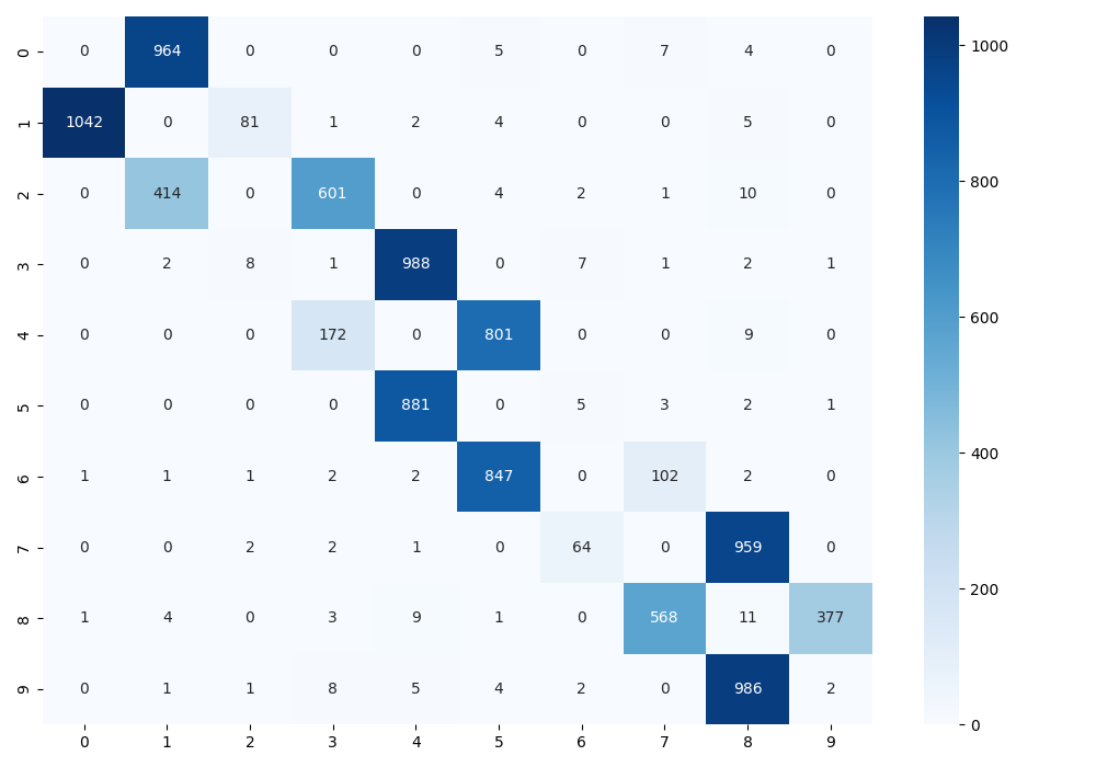
Figure 9: Confusion matrix on the MNIST classification for a local minimum

Figure 9 shows one of the confusion matrices for a model stuck in the local minimum: the CNN recognizes each digit either as the correct digit minus one or plus one. Then, our model obtains the correct prediction in close to 50% of the cases. For example, suppose the digits are a 3 and a 5. The 3 is classified either as either a 2 or a 4, while the 5 is classified as a 4 or a 6. If the model predicts 2 and 6 or 4 and 4, it returns the correct sum (8), otherwise, it does not. We believe that in these local minima there is no way for the model to change the digit predictions without increasing the loss, and the model remains stuck in the local minimum.

Table 2 shows the results in terms of accuracy of ILR, LTN Badreddine et al. (2022) and DeepProblog Manhaeve et al. (2018). To calculate the accuracy, we follow Badreddine et al. (2022) and select only the models that do not stop in the local minimum. Notice that this problem is very rare for ILR (once every 30 runs) and happens more frequently with LTN (once every 5 runs).

10 Conclusion and Future Work

We analytically studied a large class of minimal fuzzy refinement functions. We used refinement functions to construct ILR, an efficient algorithm for general formulas. Another benefit of these analytical results is to get a good intuition into what kind of corrections are done by each t-norm. In our experimental evaluation of this algorithm, we found that our algorithm converges much faster and often finds better solutions than the baseline ADAM, especially for problems that are less constraining. However, for complicated formulas and the product logic, we conclude ADAM finds better results. Finally, we assess ILR on the MNIST Addition task and show it can be combined with a neural network, providing results similar to two of the most prominent methods for neuro-symbolic AI.

There is a lot of opportunity for future work on refinement functions. We will study how the refinement functions induced by different t-norms perform in practical neuro-symbolic integration settings. On the theoretical side, possible future work could be considering analytical refinement functions for certain classes of complex formulas. Furthermore, there are many classes of t-norms and norms for which finding analytical refinement functions is an open problem. Another promising avenue for research is designing specialized loss functions that handle biases in the gradients arising from combining constrained output layers with cross-entropy loss functions Giunchiglia and Lukasiewicz (2021). We also want to highlight the possibility of extending the work on fuzzy refinement functions to probabilistic refinement functions, using a notion of minimality such as the KL-divergence.

Appendix A Basic T-norms (Proofs)

A.1 Gödel t-norm minimal refined function proofs

A.1.1 Gödel t-norm

Proposition 10.

The minimal refinement function of the Gödel t-norm for ${\hat{t}_{T_{G}}}\in[T_{G}({\bm{t}},{\bm{c}}),\min_{i=1}^{m}C_{i}]$ is

$$\rho^{*}_{T_{G}}({\bm{t}},{\hat{t}_{T_{G}}})_{i}=\begin{cases}{\hat{t}_{T_{G}}}&\text{if }t_{i}<{\hat{t}_{T_{G}}},\\ t_{i}&\text{otherwise}\end{cases}$$ (21)

Proof: Assume otherwise. Then there is a refined vector ${\hat{{\bm{t}}}}$ for $T_{G}$, ${\bm{t}}\in[0,1]^{n}$ and ${\hat{t}_{T_{G}}}\in[T_{G}({\bm{t}}),\min_{i=1}^{m}]$ such that ${\hat{{\bm{t}}}}\neq{{\bm{t}}^{*}}$ while $\|{\hat{{\bm{t}}}}-{\bm{t}}\|_{p}<\|{{\bm{t}}^{*}}-{\bm{t}}\|_{p}$, where ${{\bm{t}}^{*}}=\rho^{*}_{T_{G}}({\bm{t}},{\hat{t}_{T_{G}}})$. Since $T_{G}({\hat{{\bm{t}}}})={\hat{t}_{T_{G}}}$, for all $i\in\{1,...,n\}$, ${\hat{t}}_{i}\geq{\hat{t}_{T_{G}}}$ and so necessarily for all $i$ such that $t_{i}<{\hat{t}_{T_{G}}}$, ${\hat{t}}_{i}\geq{\hat{t}_{T_{G}}}$. Since there is some $i$ such that ${\hat{t}}_{i}\neq{t^{*}}_{i}$, either $t_{i}<{\hat{t}_{T_{G}}}$ and then necessarily ${\hat{t}}_{i}>{t^{*}}_{i}$, or ${\hat{t}}_{i}\geq{\hat{t}_{T_{G}}}$ but ${\hat{t}}_{i}\neq{t^{*}}_{i}=t_{i}$. In either case, since $\|\cdot\|_{p}$ is strictly convex in each argument with minimum at ${\bm{t}}$, $\|{\hat{{\bm{t}}}}-{\bm{t}}\|_{p}>\|{{\bm{t}}^{*}}-{\bm{t}}\|_{p}$, hence ${\hat{{\bm{t}}}}$ could not have smaller norm.

A.1.2 Gödel t-conorm

A derivation for increasing the Gödel t-conorm was first presented in Daniele and Serafini [2019] and is adapted to our notation here:

Proposition 11.

The minimal refinement function of the Gödel t-conorm for ${\hat{t}_{S_{G}}}\in[S_{G}({\bm{t}},{\bm{c}}),1]$ is

$$\rho^{*}_{S_{G}}({\bm{t}},{\hat{t}_{S_{G}}})_{i}=\begin{cases}{\hat{t}_{S_{G}}}&\text{if }i=\arg\max_{j=1}^{n}t_{j}\\ t_{i}&\text{otherwise.}\end{cases}$$ (22)

A.1.3 Gödel Implication

We next present a proof for Proposition 4.

Proof: First, assume ${\hat{t}_{R_{G}}}<1$. To ensure $R_{G}(t_{1},t_{2})={\hat{t}_{R_{G}}}$, we require $t_{2}={\hat{t}_{R_{G}}}$ as is clear from the definition. However, we also require $t_{1}>{\hat{t}_{R_{G}}}$. If $t_{1}$ is already larger, we can leave it to ensure minimality. Otherwise, we require it to be at least infinitesimally bigger, that is ${\hat{t}_{R_{G}}}+\epsilon$.

Next, assume ${\hat{t}_{R_{G}}}=1$. If $t_{1}\leq t_{2}$, then the implication is already 1 and we do not need to revise anything. Otherwise, setting it equal to any value between $t_{2}$ and $t_{1}$ is minimal.

A.2 Łukasiewicz t-norm minimal refined function proofs

A.2.1 Łukasiewicz t-norm

Proposition 12.

Let ${\hat{t}_{T_{L}}}\in[T_{L}({\bm{t}},{\bm{c}}),\max(\|{\bm{c}}\|_{1}-(m-1),0)]$ and define $\lambda_{K}=\frac{{\hat{t}_{T_{L}}}+m+K-1-\|{\bm{c}}\|_{1}-\sum_{i=1}^{K}t^{\uparrow}_{i}}{K}$. Let $K^{*}$ be the largest integer $1\leq K\leq|D|$ such that $\lambda_{K}<1-t^{\uparrow}_{K}$. Then the minimal refinement vector of the Łukasiewicz t-norm is

$$\rho^{*}_{T_{L}}({\bm{t}},{\hat{t}_{T_{L}}})_{i}=\begin{cases}t_{i}+\lambda_{K^{*}}&\text{if }t_{i}\leq t^{\uparrow}_{K},\\ 1&\text{otherwise}\end{cases}$$ (23)

Proof: We will prove this using the KKT conditions, which are both necessary and sufficient for minimality for the Łukasiewicz t-norm since it is affine when the max constraint is not active. We drop the $p$-root in the norm since it is a strictly monotonically increasing function. The Lagrangian and corresponding derivative is

$$\ell =\sum_{i=1}^{n}|{\hat{t}}_{i}-t_{i}|^{p}+\lambda(\max(\|{\hat{{\bm{t}}}}\|_{1}+\|{\bm{c}}\|_{1}-(m+n-1),0)-{\hat{t}_{T_{L}}})+\sum_{i=1}^{n}\gamma_{i}({\hat{t}}_{i}-1)$$

$$\frac{\partial\ell}{\partial{\hat{t}}_{i}} =p({\hat{t}}_{i}-t_{i})^{p-1}+\lambda\frac{\partial}{\partial{\hat{t}}_{i}}\max(\|{\hat{{\bm{t}}}}\|_{1}+\|{\bm{c}}\|_{1}-(m+n-1),0)+\gamma_{i}=0.$$

We note that we drop the absolute signs since $T_{L}$ is strictly monotonically increasing function and ${\hat{t}_{T_{L}}}\geq T_{L}({\bm{t}},{\bm{c}})$. Assuming ${\hat{t}_{T_{L}}}>0$, $T_{L}({\hat{{\bm{t}}}},{\bm{c}})={\hat{t}_{T_{L}}}$ can only be true if the first argument of $\max$ is chosen. Then for all $i,j\in\{1,...,n\}$, $p({\hat{t}}_{i}-t_{i})^{p-1}+\gamma_{i}=p({\hat{t}}_{j}-t_{j})^{p-1}+\gamma_{j}$. Define $I$ as the set of $K^{*}$ smallest $t_{i}$.

• Primal feasibility: For all $i\in I$, $\rho^{*}_{T_{L}}({\bm{t}},{\hat{t}_{T_{L}}})_{i}=\lambda_{K^{*}}\leq 1$ by definition. For all $i\in\{1,...,n\}\setminus I$, $\rho^{*}_{T_{L}}({\bm{t}},{\hat{t}_{T_{L}}})_{i}=1-t_{i}$. Furthermore,

  $$T_{L}(\rho^{*}_{T_{L}}({\bm{t}},{\hat{t}_{T_{L}}}),{\bm{c}}) =\max(\sum_{i=1}^{K^{*}}(t^{\uparrow}_{i}+\lambda_{K^{*}})+\sum_{i=K^{*}+1}^{n}1+\|{\bm{c}}\|_{1}-n-m+1,0)$$

  $$=\max(\sum_{i=1}^{K^{*}}t^{\uparrow}_{i}+K^{*}\lambda_{K^{*}}+n-K^{*}+\|{\bm{c}}\|_{1}-n-m+1,0)$$

  $$=\max(\sum_{i=1}^{K^{*}}t_{i}^{\uparrow}+{\hat{t}_{T_{L}}}+m+K^{*}-1-\|{\bm{c}}\|_{1}-\sum_{i=1}^{K^{*}}t^{\uparrow}_{i}$$

  $$-K^{*}+\|{\bm{c}}\|_{1}-m+1,0)={\hat{t}_{T_{L}}}$$

• Complementary Slackness: Clearly, for all $i\in I$, we require $\gamma_{i}=0$. For all $i\in\{1,...,n\}\setminus I$, $\rho^{*}_{T_{L}}({\bm{t}},{\hat{t}_{T_{L}}}t)_{i}-1=1-1=0$.

• Dual feasibility: For all $i\in I$, $\gamma_{i}=0$. For $i\in\{1,...,n\}\setminus I$, consider some $j\in I$ and note that $p({\hat{t}}_{i}-t_{i})^{p-1}+\gamma_{i}=p({\hat{t}}_{j}-t_{j})^{p-1}+\gamma_{j}$. Filling in ${\hat{{\bm{t}}}}$, we find $\gamma_{i}=p\lambda_{K^{*}}^{p-1}-p(1-t_{i})^{p-1}$. This is nonnegative if $\lambda_{K^{*}}\geq 1-t_{i}$. First, we show $\lambda_{K^{*}}\geq\lambda_{K^{*}+1}$. Write out their definitions, multiply by $K^{*}(K^{*}+1)$ and remove common terms. Then,

  $${\hat{t}_{T_{L}}}+m-1-\|{\bm{c}}\|_{1}-\sum_{i=1}^{K^{*}}t_{i}^{\uparrow} \geq-K^{*}t^{\uparrow}_{K^{*}+1}$$

  $${\hat{t}_{T_{L}}}+m+K^{*}+1-\|{\bm{c}}\|_{1}-\sum_{i=1}^{K^{*}+1}t_{i}^{\uparrow} \geq(K^{*}+1)(1-t_{K^{*}+1}^{\uparrow})$$

  $$\lambda_{K^{*}+1} \geq 1-t_{K^{*}+1}^{\uparrow}.$$

  $\lambda_{K^{*}+1}\geq 1-t_{K^{*}+1}^{\uparrow}$ is true by the construction in the proposition. Therefore,

  $$\lambda_{K^{*}}\geq\lambda_{K^{*}+1}\geq 1-t^{\uparrow}_{K^{*}+1}\geq 1-t_{i},$$

  proving dual feasibility.

A.2.2 Łukasiewicz t-conorm

Proposition 13.

The minimal refinement function of the Łukasiewicz t-conorm for ${\hat{t}_{S_{L}}}\in[S_{L}({\bm{t}},{\bm{c}}),{\hat{t}_{S_{L}}}]$ is

$$\rho^{*}_{S_{L}}({\bm{t}},{\hat{t}_{S_{L}}})_{i}=t_{i}+\frac{\max({\hat{t}_{S_{L}}}-\|{\bm{t}}\|_{1}-\|{\bm{c}}\|_{1},0)}{n}$$ (24)

Proof: We do not add multipliers for the constraints on ${\hat{t}}_{i}$, and show critical points adhere to these constraints. The Lagrangian is

$$\ell=\sum_{i=1}^{n}({\hat{t}}_{i}-t_{i})^{p}+\lambda(\min(\|{\hat{{\bm{t}}}}\|_{1}+\|{\bm{c}}\|_{1},1)-{\hat{t}_{S_{L}}})$$ (25)

Note that ${\max_{S_{L}}}=1$. Taking the derivative to ${\hat{t}}_{i}$, we find

$$\frac{\partial\ell}{\partial{\hat{t}}_{i}}=p\cdot({\hat{t}}_{i}-t_{i})^{p-1}+\lambda\frac{\partial}{\partial{\hat{t}}_{i}}\min(\min(\|{\hat{{\bm{t}}}}\|_{1}+\|{\bm{c}}\|_{1},1)=0$$

Assume ${\hat{t}_{S_{L}}}\neq S_{L}({\bm{t}})$, this gives three cases for all $i\in\{1,...,n\}$:

1. If $\|{\bm{t}}\|_{1}+\|{\bm{c}}\|\geq 1$ and ${\hat{t}_{S_{L}}}=1$, then since ${\hat{t}}_{i}\geq t_{i}$, $\frac{\partial}{\partial{\hat{t}}_{i}}\min(\|{\hat{{\bm{t}}}}\|_{1}+\|{\bm{c}}\|_{1},1)=\frac{\partial}{\partial{\hat{t}}_{i}}1=0$, and so ${\hat{t}}_{i}=t_{i}$.

2. If $\|{\bm{t}}\|_{1}+\|{\bm{c}}\|\geq 1$, then ${\min_{S_{L}}}={\max_{S_{L}}}=1$, and again ${\hat{t}}_{i}=t_{i}$.

3. Otherwise, it must be that $\|{\hat{{\bm{t}}}}\|_{1}+\|{\bm{c}}\|_{1}\leq 1$ and so $\frac{\partial}{\partial{\hat{t}}_{i}}\min(\|{\hat{{\bm{t}}}}\|_{1}+\|{\bm{c}}\|_{1},1)=\frac{\partial}{\partial{\hat{t}}_{i}}\|{\hat{{\bm{t}}}}\|_{1}=1$, and therefore $p\cdot({\hat{t}}_{i}-t_{i})^{p-1}=-\lambda$. Since the equality holds for all $i\in\{1,...,n\}$, we find $p\cdot({\hat{t}}_{i}-t_{i})^{p-1}=p\cdot({\hat{t}}_{j}-t_{j})^{p-1}$ for all $i,j\in\{1,...,n\}$. As we are only interested in real nonnegative solutions, we find that ${\hat{t}}_{i}-t_{i}={\hat{t}}_{j}-t_{j}=\delta$. Since $\|{\hat{{\bm{t}}}}\|_{1}+\|{\bm{c}}\|_{1}=\|{\bm{t}}\|_{1}+\|{\bm{c}}\|_{1}+n\delta={\hat{t}_{S_{L}}}$, we find

   $$\delta=\frac{{\hat{t}_{S_{L}}}-\|{\bm{t}}\|_{1}-\|{\bm{c}}\|_{1}}{n},\quad{\hat{t}}_{i}=t_{i}+\delta.$$

   Note that ${\hat{t}}_{i}\geq t_{i}$, since by assumption ${\hat{t}_{S_{L}}}\geq S_{L}({\bm{t}},{\bm{c}})$, and ${\hat{t}}_{i}\leq 1$ since by ${\hat{t}_{S_{L}}}\leq{\max_{S_{L}}}\leq 1$, $\delta=\frac{{\hat{t}_{S_{L}}}-\|{\bm{t}}\|_{1}-\|{\bm{c}}\|_{1}}{n}\leq\frac{1-\|{\bm{t}}\|_{1}-\|{\bm{c}}\|_{1}}{n}\leq\frac{1-t_{i}}{n}\leq 1-t_{i}$, that is, the constraints of Equation 7 are satisfied.

Appendix B Dual Problem

This section introduces a dual problem to Equation 7. This is used extensively in several proofs.

B.1 Strict cone monotonicity

Definition 10.

A set $K\subset[0,1]^{n}$ is a (convex) cone if for every $s>0$ and ${\bm{t}}\in K$ such that $s{\bm{t}}\in[0,1]^{n}$, also $s{\bm{t}}\in K$.

A fuzzy evaluation operator $f_{\varphi}$ is strictly cone-increasing at ${\bm{t}}\in[0,1]^{n}$ if there is a nonempty cone $K({\bm{t}})$ such that ${\bm{t}}^{\prime}-{\bm{t}}\in K$ implies $f_{\varphi}({\bm{t}})<f_{\varphi}({\bm{t}}^{\prime})$.

Strict cone-monotonicity is a weak notion of monotonicity in the sense that all t-norms that are strictly increasing in each argument are strictly cone-increasing, but the reverse need not be true.

Proposition 14.

If $f_{\varphi}$ is non-decreasing and strictly cone-increasing at ${\bm{t}}\in[0,1]^{n}$, there exist a nonempty cone $K^{\prime}({\bm{t}})\subseteq K({\bm{t}})$ such that ${\bm{t}}^{\prime}-{\bm{t}}\in K^{\prime}({\bm{t}})$ implies ${\bm{t}}^{\prime}_{i}\geq t_{i}$ for all $i\in\{0,...,n\}$.

Proof: Assume otherwise. Consider some ${\bm{t}}^{\prime}$ such that $s({\bm{t}}^{\prime}-{\bm{t}})\in K({\bm{t}})$ for $s>0$. By assumption, there is some $i\in\{0,...,n\}$ such that ${\bm{t}}^{\prime}_{i}<t_{i}$. Consider $\hat{{\bm{t}}}$ equal to ${\bm{t}}^{\prime}$ except that $\hat{{\bm{t}}}_{i}=t_{i}$ for such $i$. Since $f_{\varphi}$ is non-decreasing in each argument, $f_{\varphi}(\hat{{\bm{t}}})\geq f_{\varphi}({\bm{t}}^{\prime})>f_{\varphi}({\bm{t}})$, then clearly $s(\hat{{\bm{t}}}-{\bm{t}})$ for $s>0$ forms the cone $K^{\prime}({\bm{t}})$.

B.2 Dual problem

Next, we will investigate a dual problem for the problem in Equation 7 that will allow us to prove multiple useful theorems:

For all $${\bm{t}}\in[0,1]^{n},u\in[0,\infty):$$ (26)

$$\max_{{\hat{{\bm{t}}}}} f_{\varphi}({\hat{{\bm{t}}}})$$

such that $$\|{\hat{{\bm{t}}}}-{\bm{t}}\|=u,$$

$$0\leq{\hat{t}}_{i}\leq 1.$$

That is, instead of finding the ${\hat{{\bm{t}}}}$ closest to ${\bm{t}}$ with refinement value ${\hat{t}_{\varphi}}$, we find the largest refined value attainable with a fixed budget $u$. We need to be precise when solutions of this dual problem coincide with the problem in Equation 7. We consider strict cone-monotonicity Van Dyke et al. [2013], Clarke et al. [1993], which is a weak notion of strict monotonicity for higher dimensions. This intuitively means that there is always some direction we can move in to increase the value of the t-norm. Since t-norms are already non-decreasing in each argument, this implies there is no point where the t-norm is “flat” in all directions. The precise definition is given in Definition 10.

Theorem 3.

A solution ${{\bm{t}}^{*}}$ for some $f_{\varphi}$, ${\bm{t}}$ and $u\geq 0$ of Equation 26 is also a solution to Equation 7 for ${\bm{t}}$ and ${\hat{t}_{\varphi}}=f_{\varphi}({{\bm{t}}^{*}})\geq f_{\varphi}({\bm{t}})$ if $f_{\varphi}$ is non-decreasing in all arguments and strictly cone-increasing at each ${\bm{t}}^{\prime}\in[0,1]^{n}$ such that $f_{\varphi}({\bm{t}}^{\prime})={\hat{t}_{\varphi}}$, and if $\|\cdot\|$ is strictly increasing in all arguments.

Proof: Assume otherwise, and suppose a solution ${\hat{{\bm{t}}}}$ for Equation 7 exists such that $f_{\varphi}({\hat{{\bm{t}}}})={\hat{t}_{\varphi}}$ while $\|{\hat{{\bm{t}}}}-{\bm{t}}\|<\|{{\bm{t}}^{*}}-{\bm{t}}\|=u$. Since $f_{\varphi}$ is non-decreasing in all arguments and ${\hat{t}_{\varphi}}\geq f_{\varphi}({\bm{t}})$, ${\hat{{\bm{t}}}}-{\bm{t}}$ and ${{\bm{t}}^{*}}-{\bm{t}}$ are nonnegative. By Proposition 14 there is some cone $K({\hat{{\bm{t}}}})$ that contains a line segment $\bm{\epsilon}(s)=s({\bm{t}}^{\prime}-{\hat{{\bm{t}}}})$ such that for all $s>0$, $f_{\varphi}({\hat{{\bm{t}}}})<f_{\varphi}({\hat{{\bm{t}}}}+\mathbf{\epsilon}(s))$ and for all $i\in\{0,...,n\}$, $0\leq\bm{\epsilon}(s)_{i}$. Therefore, necessarily there is some $i$ such that $0<\bm{\epsilon}(s)_{i}$. Since $\|\cdot\|$ is strictly increasing on nonnegative vectors and continuous (since it is a norm), necessarily there is some $s>0$ such that $\|{\hat{{\bm{t}}}}+\bm{\epsilon}(s)\|=u$. However, this is in contradiction with the premise that ${{\bm{t}}^{*}}$ is a solution of Equation 26, as $f_{\varphi}({\hat{{\bm{t}}}}+\epsilon(s))>f_{\varphi}({{\bm{t}}^{*}})$.

Since $f_{\varphi}\in[0,1]^{n}\rightarrow[0,1]$, $f_{\varphi}$ cannot satisfy the conditions of Theorem 3 when ${\hat{t}_{\varphi}}=1$. For all ${\hat{t}_{\varphi}}\in[0,1)$ however, both the Gödel and product t-norms and t-conorms are strictly cone-increasing. The Łukasiewicz t-norm satisfies the conditions for ${\hat{t}_{\varphi}}\in(0,1)$, since it has flat regions for ${\hat{t}_{\varphi}}=0$. The same reasoning can be made for the nilpotent minimum and drastic t-norms, see van Krieken et al. [2022]. Furthermore, all t-norms with an additive generator are strictly cone-increasing on ${\hat{t}_{\varphi}}\in(0,1)$, as are all strict t-norms.

Appendix C Schur-concave t-norms (Proofs)

C.1 Minimal refinement function for t-norms

Theorem 4.

Let $T$ be a Schur-concave t-norm that is strictly cone-increasing at ${\hat{t}_{T}}$ and let $\|\cdot\|$ be a strict norm. Then there is a minimal refined vector ${{\bm{t}}^{*}}$ for ${\bm{t}}$ and ${\hat{t}_{T}}$ such that whenever $t_{i}>t_{j}$, then ${t^{*}}_{i}-t_{i}\leq{t^{*}}_{j}-t_{j}$.

Proof: Assume there is a minimal refined vector ${\hat{{\bm{t}}}}\neq{{\bm{t}}^{*}}$ which has some ${\hat{t}}_{i}-t_{i}>{\hat{t}}_{j}-t_{j}$ while $t_{i}>t_{j}$. Consider ${\hat{{\bm{t}}}}^{\prime}$ equal to ${\hat{{\bm{t}}}}$ except that ${\hat{t}}^{\prime}_{i}={\hat{t}}_{j}-t_{j}+t_{i}$ and ${\hat{t}}^{\prime}_{j}={\hat{t}}_{i}-t_{i}+t_{j}$ such that by symmetry $\|{\hat{{\bm{t}}}}-{\bm{t}}\|=\|{\hat{{\bm{t}}}}^{\prime}-{\bm{t}}\|$. Define ${\hat{t}}_{\max}^{\prime}=\max({\hat{t}}_{i}^{\prime},{\hat{t}}_{j}^{\prime})$ and ${\hat{t}}_{\min}^{\prime}=\min({\hat{t}}_{i}^{\prime},{\hat{t}}_{j}^{\prime})$. Clearly, ${\hat{t}}_{i}>{\hat{t}}_{\max}^{\prime}\geq{\hat{t}}_{\min}^{\prime}>{\hat{t}}_{j}$. We will show ${\hat{{\bm{t}}}}$ majorizes ${\hat{{\bm{t}}}}^{\prime}$ by checking the condition of Definition 8 for any $k\in\{1,...,n\}$.

1. If ${\hat{t}}^{\downarrow}_{k}>{\hat{t}}_{i}$, then all elements are equal and $\sum_{l=1}^{k}{\hat{t}}^{\downarrow}_{l}=\sum_{l=1}^{k}{\hat{t}}^{\prime\downarrow}_{l}$.

2. If ${\hat{t}}_{i}\geq{\hat{t}}^{\downarrow}_{k}>{\hat{t}}_{\max}^{\prime}$, then $\sum_{l=1}^{k}{\hat{t}}^{\downarrow}_{l}=\sum_{l=1}^{k-1}{\hat{t}}^{\prime\downarrow}_{l}+{\hat{t}}_{i}\geq\sum_{l=1}^{k}{\hat{t}}^{\prime\downarrow}_{l}$.

3. If ${\hat{t}}_{\max}^{\prime}\geq{\hat{t}}^{\downarrow}_{k}>{\hat{t}}_{\min}^{\prime}$, then $\sum_{l=1}^{k}{\hat{t}}^{\downarrow}_{l}>\sum_{l=1}^{k}{\hat{t}}^{\prime\downarrow}_{l}$, since by removing common terms we get ${\hat{t}}_{i}>{\hat{t}}_{\max}^{\prime}$.

4. If ${\hat{t}}_{\min}^{\prime}\geq{\hat{t}}^{\downarrow}_{k}>{\hat{t}}_{j}$, then removing all common terms in the sums, we are left with ${\hat{t}}_{i}+{\hat{t}}^{\downarrow}_{k}>{\hat{t}}_{\min}^{\prime}+{\hat{t}}_{\max}^{\prime}$. Note ${\hat{t}}_{\min}^{\prime}+{\hat{t}}_{\max}^{\prime}={\hat{t}}_{j}+t_{i}-t_{j}+{\hat{t}}_{i}+t_{j}-t_{i}={\hat{t}}_{i}+{\hat{t}}_{j}$. Subtracting ${\hat{t}}_{i}$ from both sides, we are left with ${\hat{t}}^{\downarrow}_{k}>{\hat{t}}_{j}$, which is true by assumption.

5. If ${\hat{t}}_{\min}\geq{\hat{t}}^{\downarrow}_{k}$, then removing common terms, we are left with ${\hat{t}}_{\max}+{\hat{t}}_{\min}={\hat{t}}_{i}+{\hat{t}}_{j}$.

Therefore, ${\hat{{\bm{t}}}}$ majorizes ${\hat{{\bm{t}}}}^{\prime}$, and so by Schur concavity, $T({\hat{{\bm{t}}}},{\bm{c}})\leq T({\hat{{\bm{t}}}}^{\prime},{\bm{c}})$, noting that the additional truth vector ${\bm{c}}$ will not influence the majorization result since it is applied at both sides. By Theorem 3, either 1) $T({\hat{{\bm{t}}}},{\bm{c}})<T({\hat{{\bm{t}}}}^{\prime},{\bm{c}})$, so ${\hat{{\bm{t}}}}$ could not have been minimal, leading to a contradiction, or 2) $T({\hat{{\bm{t}}}},{\bm{c}})=T({\hat{{\bm{t}}}}^{\prime},{\bm{c}})$ and both ${\hat{{\bm{t}}}}$ and ${\hat{{\bm{t}}}}^{\prime}$ are minimal.

C.2 Closed-form refinement function using additive generators

Proposition 15.

Let $T$ be a Schur-concave t-norm with additive generator $g$ and let $0<{\hat{t}_{T}}\in[T({\bm{t}},{\bm{c}}),{\max_{T}}]$. Let $K\in\{0,...,n-1\}$ denote the number of truth values such that ${t^{*}}_{i}=t_{i}$ in Equation 28. Then using

$$\lambda_{K}=g^{-1}\left(\frac{1}{n-K}\left(g({\hat{t}_{T}})-\sum_{i=1}^{K}g(t^{\downarrow}_{i})-\sum_{i=1}^{m}g(C_{i})\right)\right)$$ (27)

in Equation 28 gives $T({{\bm{t}}^{*}},{\bm{c}})={\hat{t}_{T}}$ if ${{\bm{t}}^{*}}\in[0,1]^{n}$.

Proof: Using Equations 15 and 28, we find that

$$T({{\bm{t}}^{*}},{\bm{c}})=g^{-1}\left(\min\left(g(0^{+}),\sum_{i=1}^{K}g(t^{\downarrow}_{i})+\sum_{i=K+1}^{n}g(\lambda_{K})+\sum_{i=1}^{m}g(C_{i})\right)\right)={\hat{t}_{T}}$$

Since ${\hat{t}_{T}}>0$, we can remove the $\min$, since ${\hat{t}_{T}}>0$ will require that $\sum_{i=1}^{K}g(t^{\downarrow}_{i})+(n-K)g(\lambda_{K})+\sum_{i=1}^{m}g(C_{i})>g(0^{+})$. We apply $g$ to both sides of the equation, which is allowed since $g$ is a bijection. Thus

$$g({\hat{t}_{T}}) =\sum_{i=1}^{K}g(t^{\downarrow}_{i})+(n-K)g(\lambda_{K})+\sum_{i=1}^{m}g(C_{i})$$

$$g(\lambda_{K}) =\frac{1}{n-K}\left(g({\hat{t}_{T}})-\sum_{i=1}^{K}g(t^{\downarrow}_{i})-\sum_{i=1}^{m}g(C_{i})\right)$$

$$\lambda_{K} =g^{-1}\left(\frac{1}{n-K}\left(g({\hat{t}_{T}})-\sum_{i=1}^{K}g(t^{\downarrow}_{i})-\sum_{i=1}^{m}g(C_{i})\right)\right),$$

where in the last step we apply $g^{-1}$. In a similar manner we can find the $\lambda$ for the t-conorm. Let $j={\arg\max}_{i=1}^{n}t_{i}$.

$$S({{\bm{t}}^{*}})=1-g^{-1}(\min(g(0^{+}),\sum_{i=1}^{n}g(1-{t^{*}}_{i})+\sum_{i=1}^{m}g(1-C_{i}))) ={\hat{t}_{S}}$$

$$\min(g(0^{+}),g(1-\lambda)+\sum_{i\neq j}g(1-t_{i})+\sum_{i=1}^{m}g(1-C_{i})) =g(1-{\hat{t}_{S}})$$

If ${\hat{t}_{S}}<1$, or if $g(0)$ is well defined, then we can ignore the $\min$:

$$g(1-\lambda) =g(1-{\hat{t}_{S}})-\sum_{i\neq j}g(1-t_{i}))-\sum_{i=1}^{m}g(1-C_{i})$$

$$\lambda =1-g^{-1}\left(g(1-{\hat{t}_{S}})-\sum_{i\neq j}g(1-t_{i})-\sum_{i=1}^{m}g(1-C_{i})\right)$$

C.3 L1 minimal refinement function for t-norms

Proposition 16.

Let ${\bm{t}}\in[0,1]^{n}$ and let $T$ be a Schur-concave t-norm that is strictly cone-increasing at ${\hat{t}_{T}}\in[T({\bm{t}},{\bm{c}}),{\max_{T}}]$. Then there is a value $\lambda\in[0,1]$ such that the vector ${{\bm{t}}^{*}}$,

$${t^{*}}_{i}=\begin{cases}\lambda,&\text{if }t_{i}<\lambda,\\ t_{i},&\text{otherwise,}\end{cases}$$ (28)

is a minimal refined vector for $T$ and the L1 norm at ${\bm{t}}$ and ${\hat{t}_{T}}$.

Proof: Assume otherwise. Then, using Theorem 3, there must be a refined vector ${\hat{{\bm{t}}}}$ such that $\|{\hat{{\bm{t}}}}-{\bm{t}}\|_{1}=\|{{\bm{t}}^{*}}-{\bm{t}}\|_{1}$ but $T({\hat{{\bm{t}}}},{\bm{c}})>T({{\bm{t}}^{*}},{\bm{c}})$. Since ${\hat{t}_{T}}\in[T({\bm{t}},{\bm{c}}),{\max_{T}}]$, we can assume ${\hat{t}}_{i}\geq t_{i}$. We define $\pi^{*}(i)$ as the permutation in descending order of ${{\bm{t}}^{*}}$. Furthermore, let $k$ be the smallest $j$ such that $t^{\downarrow}_{j}<\lambda$.

Since $\|{\hat{{\bm{t}}}}\|_{1}=\|{{\bm{t}}^{*}}\|_{1}$, by assumption of equal L1 norms of ${\hat{{\bm{t}}}}$ and ${{\bm{t}}^{*}}$, we will prove for all $i\in\{1,...,n\}$ that ${\hat{{\bm{t}}}}$ majorizes ${{\bm{t}}^{*}}$.

• If $i<k$, then $\sum_{j=1}^{i}{\hat{t}}^{\downarrow}_{j}\geq\sum_{j=1}^{i}{\hat{t}}_{\pi^{*}(j)}\geq\sum_{j=1}^{i}t_{\pi^{*}(j)}=\sum_{j=1}^{i}{t^{*}}^{\downarrow}_{j}$. The first inequality follows from the fact that there is no ordering of ${\hat{{\bm{t}}}}$ that will have a higher sum than in descending order.

• If $i\geq k$, then clearly ${t^{*}}^{\downarrow}_{i}=\lambda$. Furthermore, $\sum_{j=1}^{i}{t^{*}}^{\downarrow}_{j}=\sum_{j=1}^{k}t^{\downarrow}_{j}+(i-k)\lambda$. We will distinguish two cases:

  1. ${\hat{t}}^{\downarrow}_{i}\geq\lambda$. Then for all $j\in\{k,...,i\}$, ${\hat{t}}^{\downarrow}_{j}\geq\lambda$. Furthermore, from the previous result, $\sum_{j=1}^{k-1}{\hat{t}}^{\downarrow}_{j}\geq\sum_{j=1}^{k-1}{t^{*}}^{\downarrow}_{j}$ and so clearly $\sum_{j=1}^{i}{\hat{t}}^{\downarrow}_{j}\geq\sum_{j=1}^{i}{t^{*}}^{\downarrow}_{i}$.

  2. ${\hat{t}}^{\downarrow}_{i}<\lambda$. Then for all $j>i$, ${\hat{t}}^{\downarrow}_{j}\leq{\hat{t}}^{\downarrow}_{i}<\lambda$, and so $\sum_{j=i+1}^{n}{\hat{t}}^{\downarrow}_{j}\leq\sum_{j=i+1}^{n}{\hat{t}}^{\downarrow}_{i}=(n-i){\hat{t}}^{\downarrow}_{i}<(n-i)\lambda$. Using this, we note that

     $$\|{{\bm{t}}^{*}}\|_{1}=\sum_{j=1}^{k}t^{\downarrow}_{j}+(n-k)\lambda=\|{\hat{{\bm{t}}}}\|_{1}=\sum_{j=1}^{i}{\hat{t}}^{\downarrow}_{j}+\sum_{j=i+1}^{n}{\hat{t}}^{\downarrow}_{j}<\sum_{j=1}^{i}{\hat{t}}^{\downarrow}_{j}+(n-i)\lambda.$$

     Then, subtracting $(n-i)\lambda$ from the inequality, we find

     $$\sum_{j=1}^{i}{\hat{t}}^{\downarrow}_{j}>\sum_{j=1}^{k}t^{\downarrow}_{j}+(n-k)\lambda-(n-i)\lambda=\sum_{j=1}^{k}t^{\downarrow}_{j}+(i-k)\lambda=\sum_{j=1}^{i}{t^{*}}^{\downarrow}_{j}$$

And so, ${\hat{{\bm{t}}}}$ majorizes ${{\bm{t}}^{*}}$, and by Schur concavity of $T$, $T({\hat{{\bm{t}}}},{\bm{c}})\leq T({{\bm{t}}^{*}},{\bm{c}})$ leading to a contradiction.

C.4 L1 minimal refinement function for t-conorms

Proposition 17.

Let ${\bm{t}}\in[0,1]^{n}$ and let $S$ be a Schur-convex t-conorm that is strictly cone-increasing at ${\hat{t}_{S}}\in[S({\bm{t}},{\bm{c}}),1]$. Then there is a value $\lambda\in[0,1]$ such that the vector ${{\bm{t}}^{*}}$,

$${t^{*}}_{i}=\begin{cases}\lambda&\text{if }i={\arg\max}_{i\in D}t_{i},\\ t_{i},&\text{otherwise,}\end{cases}$$ (29)

is a minimal refined vector for $S$ and the L1 norm at ${\bm{t}}$ and ${\hat{t}_{S}}$.

Proposition 18.

Let ${\bm{t}}\in[0,1]^{n}$ and let $S$ be a Schur-convex t-conorm that is strictly cone-increasing at ${\hat{t}_{S}}\in[S({\bm{t}},{\bm{c}}),1]$. Then there is a value $\lambda\in[0,1]$ such that the vector ${{\bm{t}}^{*}}$ with $i\in D$,

$${t^{*}}_{i}=\begin{cases}\lambda&\text{if }i={\arg\max}_{i\in D}t_{i},\\ t_{i},&\text{otherwise,}\end{cases}$$ (30)

is a minimal refined vector for $S$ and the L1 norm at ${\bm{t}}$ and ${\hat{t}_{S}}$.

Proof: Assume otherwise. Then, using Theorem 3, there must be a refined vector ${\hat{{\bm{t}}}}\neq{{\bm{t}}^{*}}$ such that $\|{\hat{{\bm{t}}}}-{\bm{t}}\|_{1}=\|{{\bm{t}}^{*}}-{\bm{t}}\|_{1}=\lambda-{\bm{t}}^{\downarrow}_{1}$ but $S({\hat{{\bm{t}}}},{\bm{c}})>S({{\bm{t}}^{*}},{\bm{c}})$. Let $\pi(i)$ be the permutation in descending order of ${\hat{{\bm{t}}}}$.

Consider any $k\in\{1,...,n\}$. Then $\sum_{i=1}^{k}{t^{*}}^{\downarrow}_{i}=\sum_{i=1}^{k}t^{\downarrow}_{i}+(\lambda-t^{\downarrow}_{1})$, while $\sum_{i=1}^{k}{\hat{t}}^{\downarrow}_{j}=\sum_{i=1}^{k}t_{\pi(i)}+\sum_{i=1}^{k}({\hat{t}}_{i}-t_{\pi(i)})$. There is no permutation with higher sum than in descending order, so $\sum_{i=1}^{k}t_{\pi(i)}\leq\sum_{i=1}^{k}t^{\downarrow}_{i}$. Furthermore, since $\|{\hat{{\bm{t}}}}-{\bm{t}}\|_{1}=\lambda-t^{\downarrow}_{1}$, $\sum_{i=1}^{k}({\hat{t}}_{i}-t_{\pi(i)})\leq\lambda-t^{\downarrow}_{1}$. Therefore, $\sum_{i=1}^{k}{\hat{t}}^{\downarrow}_{i}\leq\sum_{i=1}^{k}{t^{*}}^{\downarrow}_{i}$, that is, ${{\bm{t}}^{*}}$ majorizes ${\hat{{\bm{t}}}}$, and by Schur convexity of $S$, $S({{\bm{t}}^{*}},{\bm{c}})\geq S({\hat{{\bm{t}}}},{\bm{c}})$.

C.5 L1 minimal refinement function for residuums

Proposition 19.

Let $t_{1},t_{2}\in[0,1]$ and let $T$ be a strict Schur-concave t-norm with additive generator $g$. Consider its residuum $R(t_{1},t_{2})=\sup\{z|T(t_{1},z)\leq t_{2}\}$ that is strictly cone-increasing at $0<{\hat{t}_{R}}\in[R(t_{1},t_{2}),{\max_{R}}]$. Then there is a value $\lambda\in[0,1]$ such that ${{\bm{t}}^{*}}=[t_{1},\lambda]^{\top}$ is a minimal refined vector for $R$ and the L1 norm at ${\bm{t}}$ and $t$.

Proof: We will assume $t_{1}>t_{2}$, as otherwise $R(t_{1},t_{2})=1$ for any residuum, which necessarily means ${\hat{t}_{R}}=1$ and so ${{\bm{t}}^{*}}={\bm{t}}$. Assume ${{\bm{t}}^{*}}$ is not minimal. Since $R$ is strictly cone increasing at ${\hat{t}_{R}}$, by Theorem 3 there must be some ${\hat{{\bm{t}}}}$ such that $\|{\hat{{\bm{t}}}}-{\bm{t}}\|=\|{{\bm{t}}^{*}}-{\bm{t}}\|=\lambda-t_{2}$ but $R({\hat{t}}_{1},{\hat{t}}_{2})>R({t^{*}}_{1},{t^{*}}_{2})$. Since $R$ is non-decreasing in the first argument and non-increasing in the second, we consider ${\hat{{\bm{t}}}}=[t_{1}-\epsilon,\lambda-\epsilon]^{\top}$ for $\epsilon>0$.

The residuum constructed from continuous t-norms with an additive generator can be computed as $R(t_{1},t_{2})=g^{-1}(\max(g(t_{2})-g(t_{1}),0))$. Since we assumed $R({t^{*}}_{1},{t^{*}}_{2})<R({\hat{t}}_{1},{\hat{t}}_{2})$, applying $g$ to both sides,

$$\max(g(\lambda)-g(t_{1}),0) >\max(g(\lambda-\epsilon)-g(t_{1}-\epsilon),0)$$

$$g^{-1}(g(\lambda)+g(t_{1}-\epsilon)) <g^{-1}(g(\lambda-\epsilon)+g(t_{1}))$$

$$T(\lambda,t_{1}-\epsilon) <T(\lambda-\epsilon,t_{1})$$

where in the second step we assume $\lambda\leq t_{1}$, that is, we are not setting new consequent larger than the antecedent, as otherwise we could find a smaller refined vector by setting it to exactly $t_{1}$. In the last step we use that $T$ is strict, as then $T(t_{1},t_{2})=g^{-1}(g(t_{1})+t_{2}))$. We now use the majorization as $\lambda+t_{1}-\epsilon=\lambda-\epsilon+{\bm{t}}$.

Since $\lambda\leq t_{1}$, surely $t_{1}>\lambda-\epsilon$. Then there are two cases:

1. $\lambda\geq t_{1}-\epsilon$. Then $t_{1}\geq\lambda$ as assumed.

2. $t_{1}-\epsilon\geq\lambda$. Then clearly ${\bm{t}}\geq t_{1}-\epsilon$ as $\epsilon>0$.

Therefore $[\lambda-\epsilon,t_{1}]^{\top}$ majorizes $[\lambda,{\bm{t}}-\epsilon]^{\top}$, and by Schur concavity $T(\lambda,{\bm{t}}-\epsilon)\geq T(\lambda-\epsilon,t_{1})$ which is a contradiction.

Appendix D Product t-norm with L2 norm

In this appendix, we consider the refinement functions for the product t-norm under the L2-norm. We find that there is no simple closed-form parameterization in terms of ${\hat{t}_{\varphi}}$, but we can find approximations in linear time. These are satisfactory to reliably find the minimal refinement function.

In the following, we wil ignore constants and consider formulas $\bigwedge_{i=1}^{n}P_{i}$, and consider the problem in Equation 7. We consider the logarithm of the product as its optimum coincides.

For all $${\bm{t}}\in[0,1]^{n},{\hat{t}_{T_{P}}}\in[T_{P}({\bm{t}}),1]$$ (31)

$$\min_{{\hat{{\bm{t}}}}} \sum_{i=1}^{n}({\hat{t}}_{i}-t_{i})^{2}$$

such that $$\sum_{i=1}^{n}\log{\hat{t}}_{i}=\log{\hat{t}_{T_{P}}}$$

$${\hat{t}}_{i}-1\leq 0$$

With Lagrangian $L=\sum_{i}({\hat{t}}_{i}-t_{i})^{2}+\lambda(\sum_{i}\log{\hat{t}}_{i}-\log{\hat{t}_{T_{P}}})-\gamma_{i}({\hat{t}}_{i}-1)$, and so

$$\frac{\partial L}{\partial{\hat{t}}_{i}} =2({\hat{t}}_{i}-t_{i})-\gamma_{i}+\frac{\lambda}{{\hat{t}}_{i}}=0$$

$$\lambda =(\gamma+2t_{i}-2{\hat{t}}_{i}){\hat{t}}_{i}$$

Since this holds for all $i$, we find that for all $i$, $j$, $(\gamma+2t_{i}-2{\hat{t}}_{i}){\hat{t}}_{i}=(\gamma+2t_{j}-2{\hat{t}}_{j}){\hat{t}}_{j}=\lambda$. We partition $\{1,...,n\}$ into sets $I$ and $M$, where $I$ contains all $i$ such that ${\hat{t}}_{i}<1$, and $M$ those where ${\hat{t}}_{i}=1$. For $i\in I$, by noting that using the complementary slackness condition $\gamma_{i}=0$, this induces a quadratic equation in ${\hat{t}}_{i}$ with solutions

$${\hat{t}}_{i}=\frac{1}{2}(t_{i}\pm\sqrt{t_{i}^{2}-2\lambda}).$$ (32)

Since we assume ${\hat{t}}_{i}\geq t_{i}$, we have to take the solution that adds the root of the determinant, that is, ${\hat{t}}_{i}=\frac{1}{2}(\sqrt{t_{i}^{2}-2\lambda}+t_{i})$. Furthermore, since we constrain for $i\in I$ that ${\hat{t}}_{i}<1$, we find that

$$1 >\frac{1}{2}(t_{i}+\sqrt{t_{i}^{2}-2\lambda})$$

$$2-t_{i} >\sqrt{t_{i}^{2}-2\lambda}$$

$$\lambda >2t_{i}-2.$$

Therefore, given some chosen value of $c$, we require for all $i\in I$ that $\lambda>2t_{i}-2$, and so,

$$\min_{i\in I}2t_{i}-2>\lambda$$

Unfortunately, finding the exact value of $\lambda$ such that $T_{P}({\hat{{\bm{t}}}})={\hat{t}_{T_{P}}}$ is a challenge. Filling in ${\hat{t}}_{i}$, we find

$$T_{P}({\hat{{\bm{t}}}})=\prod_{i=1}^{n}({\hat{t}}_{i})=\prod_{i\in I}\frac{1}{2}(t_{i}+\sqrt{t_{i}^{2}-2\lambda})={\hat{t}_{T_{P}}}.$$ (33)

This is a $2n$-th degree polynomial in $\lambda$, and we were not able to find an obvious, general closed form solution to it. Mathematica Inc. [2019] finds a complicated closed form formula for $n=2$, but cannot find closed form formulas for $n>2$.

We also still need to figure out how to partition $i=\{1,...,n\}$ into $I$ and $M$. Since ${\hat{t}}_{i}$ as computed by Equation 32 is a strictly decreasing function in $\lambda$ for all $i\in I$, we have the following unproven proposition. It supports the result given in Theorem 4 .

Proposition 20.

For all $\lambda\in[\min_{i=1}^{n}2t_{i}-2,0]$, the function

$$\rho^{*}_{T_{P}}({\bm{t}},\lambda)_{i}=\begin{cases}\frac{1}{2}(t_{i}+\sqrt{t_{i}^{2}-2\lambda})&\text{if }2t_{i}-2>\lambda,\\ 1-t_{i}&\text{otherwise.}\end{cases}$$ (34)

has the following properties:

1. $\rho^{*}_{T_{P}}({\bm{t}},\lambda)$ is a minimal refinement vector for the product t-norm, the L2 norm and ${\hat{t}_{T_{P}}}=T_{P}(\rho^{*}_{T_{P}}({\bm{t}},\lambda))$;

2. ${\hat{t}_{T_{P}}}=T_{P}(\rho^{*}_{T_{P}}({\bm{t}},\lambda))$ is a strictly decreasing function in $c$ on $(\min_{i=1}^{n}2t_{i}-2,0]$, and so there is a bijection between $\lambda$ and $t\in[T_{P}({\bm{t}}),1]$ on this interval.

The second property is easy to see by noting the derivative of $\rho^{*}_{T_{P}}({\bm{t}},\lambda)$ is negative on $\lambda\in(\min_{i=1}^{n}2t_{i}-2]$, but for the first we do not have a direct proof as of yet and leave this for future work.

Although $\rho^{*}_{T_{P}}({\bm{t}},\lambda)$ is not parameterized in terms of ${\hat{t}_{T_{P}}}$, it can still be used in practical scenarios where $\lambda$ can be seen as the negative “confidence” in the clause. A practical implementation could learn a weight for the clause between 0 and 1, and then transform it to the domain of $\lambda$ by dividing by $\min_{i=1}^{n}2t_{i}-2$. Alternatively, $\|T_{P}({\bm{t}}+\rho^{*}_{T_{P}}({\bm{t}},\lambda))-{\hat{t}_{T_{P}}}\|_{2}$ can be minimized with respect to $\lambda$ using mathematical optimization methods like gradient descent or Newton’s method to find answers in terms of ${\hat{t}_{T_{P}}}$.

Appendix E Additional experiments

In this Appendix we present additional experiments when ${\hat{t}_{\varphi}}$ is not 1.

E.1 Results - Refined value 0.3

The figures in this section present the results when the refined value ${\hat{t}_{\varphi}}=0.3$.

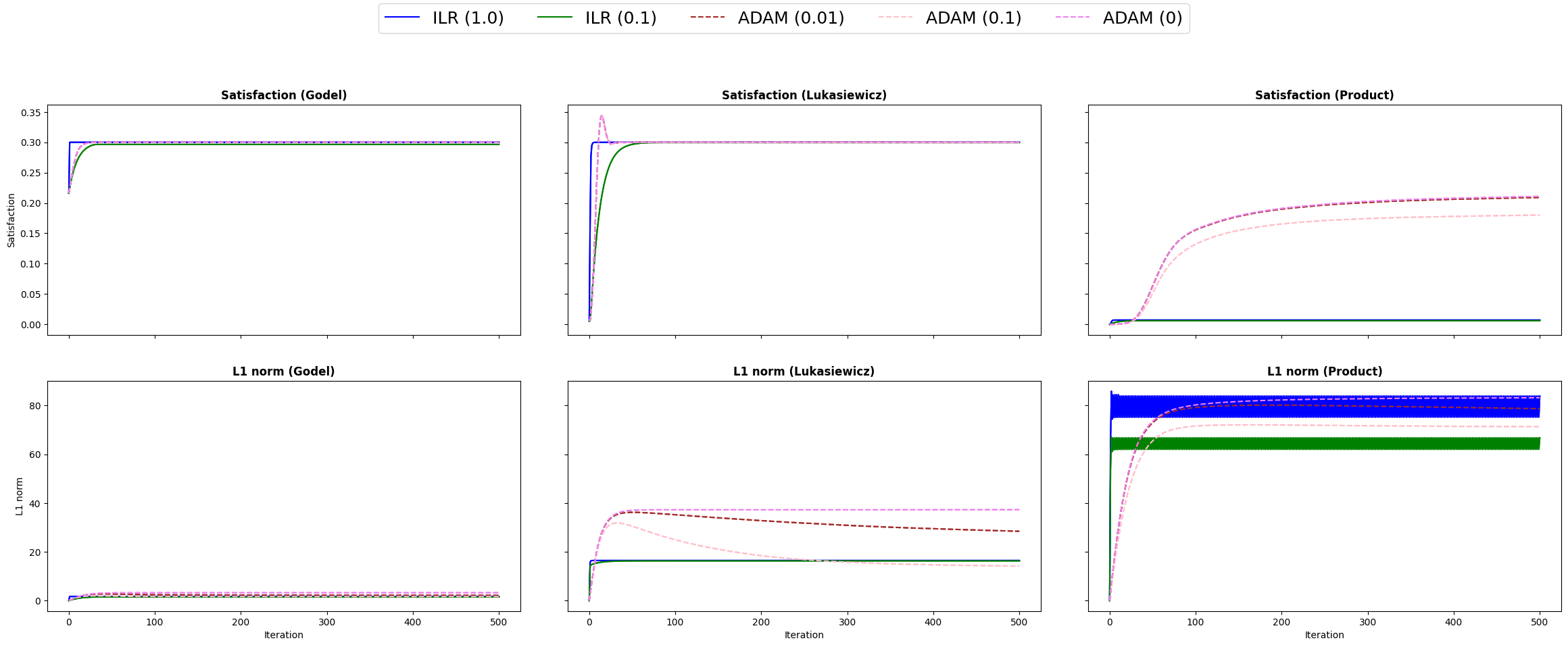
Figure 10: Comparison of ILR with ADAM on uf20-91 of SATLIB. Refined value 0.3. The x axis corresponds to the number of iterations, while the y axis is the value of ${\hat{t}_{\varphi}}$ in the first row of the grid, and the L1 norm in the second row.

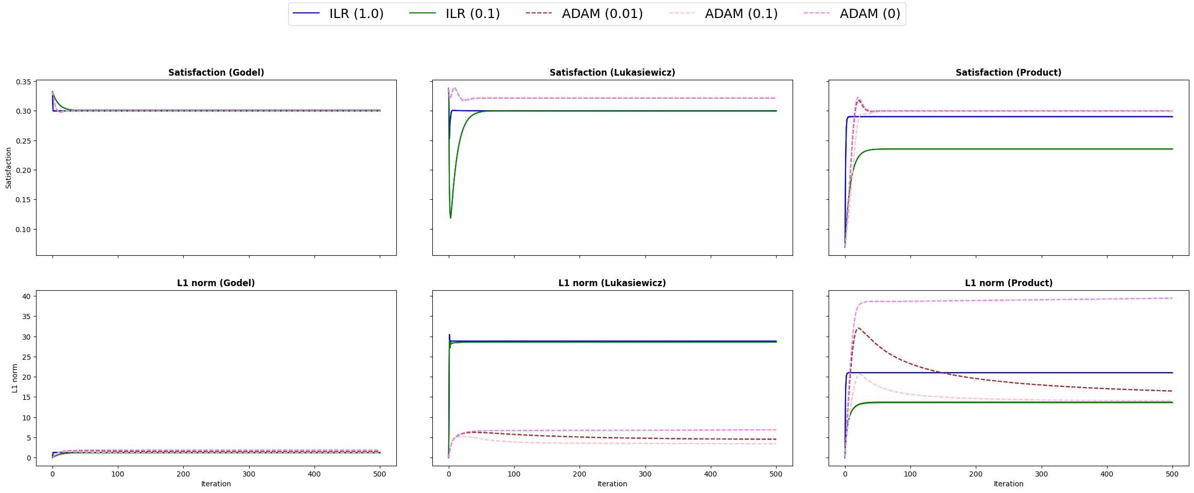
Figure 11: Comparison of ILR with ADAM on the uf20-91 with 20 clauses. Refined value 0.3.

E.2 Results - Refined value 0.5

The figures in this section present the results when the refined value ${\hat{t}_{\varphi}}=0.5$. We note that the satisfaction for ADAM in Łukasiewicz converges above 0.5 in Figure 13. This means the final truth value is too high, and it has not found a proper solution here.

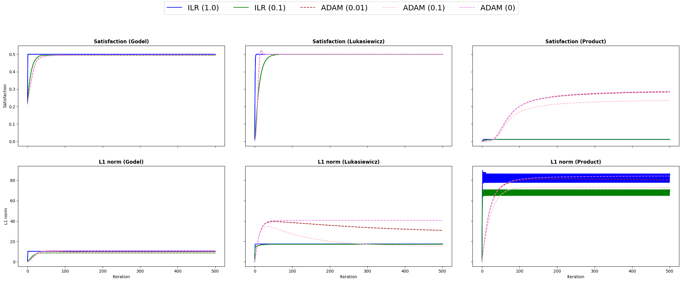
Figure 12: Comparison of ILR with ADAM on the uf20-91 of SATLIB. Refined value 0.5.

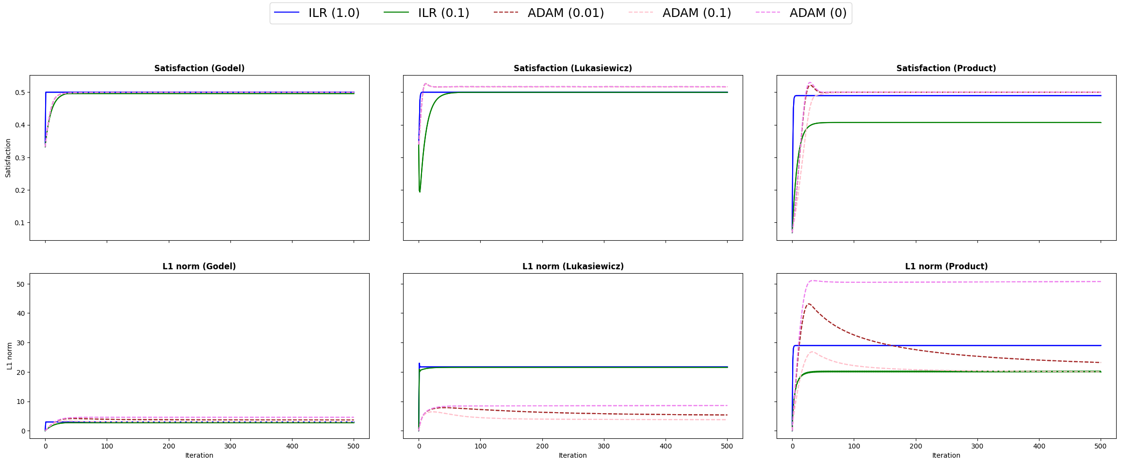
Figure 13: Comparison of ILR with ADAM on the uf20-91 with 20 clauses. Refined value 0.5.

References

- Ahmed et al. [2022] K. Ahmed, S. Teso, K.-W. Chang, G. V. den Broeck, and A. Vergari. Semantic Probabilistic Layers for Neuro-Symbolic Learning. In The 5th Workshop on Tractable Probabilistic Modeling, July 2022.
- Alsina [1984] C. Alsina. On Schur-Concave t-Norms and Triangle Functions. In W. Walter, editor, General Inequalities 4: In Memoriam Edwin F. Beckenbach 4th International Conference on General Inequalities, Oberwolfach, May 8–14, 1983, pages 241–248. Birkhäuser, Basel, 1984. ISBN 978-3-0348-6259-2. 10.1007/978-3-0348-6259-2_22.
- Badreddine et al. [2022] S. Badreddine, A. d’Avila Garcez, L. Serafini, and M. Spranger. Logic Tensor Networks. Artificial Intelligence, 303:103649, Feb. 2022. ISSN 0004-3702. 10.1016/j.artint.2021.103649.
- Calvo et al. [2002] T. Calvo, A. Kolesárová, M. Komorníková, and R. Mesiar. Aggregation operators: Properties, classes and construction methods. In T. Calvo, G. Mayor, and R. Mesiar, editors, Aggregation Operators: New Trends and Applications, pages 3–104. Physica-Verlag HD, Heidelberg, 2002. ISBN 978-3-7908-1787-4.
- Chowdhery et al. [2022] A. Chowdhery, S. Narang, J. Devlin, M. Bosma, G. Mishra, A. Roberts, P. Barham, H. W. Chung, C. Sutton, S. Gehrmann, P. Schuh, K. Shi, S. Tsvyashchenko, J. Maynez, A. Rao, P. Barnes, Y. Tay, N. Shazeer, V. Prabhakaran, E. Reif, N. Du, B. Hutchinson, R. Pope, J. Bradbury, J. Austin, M. Isard, G. Gur-Ari, P. Yin, T. Duke, A. Levskaya, S. Ghemawat, S. Dev, H. Michalewski, X. Garcia, V. Misra, K. Robinson, L. Fedus, D. Zhou, D. Ippolito, D. Luan, H. Lim, B. Zoph, A. Spiridonov, R. Sepassi, D. Dohan, S. Agrawal, M. Omernick, A. M. Dai, T. S. Pillai, M. Pellat, A. Lewkowycz, E. Moreira, R. Child, O. Polozov, K. Lee, Z. Zhou, X. Wang, B. Saeta, M. Diaz, O. Firat, M. Catasta, J. Wei, K. Meier-Hellstern, D. Eck, J. Dean, S. Petrov, and N. Fiedel. PaLM: Scaling Language Modeling with Pathways. arXiv:2204.02311 [cs], Apr. 2022.
- Clarke et al. [1993] F. H. Clarke, R. J. Stern, and P. R. Wolenski. Subgradient Criteria for Monotonicity, The Lipschitz Condition, and Convexity. Canadian Journal of Mathematics, 45(6):1167–1183, Dec. 1993. ISSN 0008-414X, 1496-4279. 10.4153/CJM-1993-065-x.
- Daniele and Serafini [2019] A. Daniele and L. Serafini. Knowledge enhanced neural networks. In A. C. Nayak and A. Sharma, editors, PRICAI 2019: Trends in Artificial Intelligence, pages 542–554, Cham, 2019. Springer International Publishing. ISBN 978-3-030-29908-8.
- Daniele and Serafini [2022] A. Daniele and L. Serafini. Knowledge enhanced neural networks for relational domains. arXiv preprint arXiv:2205.15762, 2022.
- Diligenti et al. [2017] M. Diligenti, M. Gori, and C. Sacca. Semantic-based regularization for learning and inference. Artificial Intelligence, 244:143–165, 2017.
- Donadello et al. [2017] I. Donadello, L. Serafini, and A. d’Avila Garcez. Logic tensor networks for semantic image interpretation. In IJCAI International Joint Conference on Artificial Intelligence, pages 1596—1602, 2017.
- [11] P. Dragone, S. Teso, and A. Passerini. Neuro-Symbolic Constraint Programming for Structured Prediction. page 9.
- [12] M. Fischer, M. Balunovic, D. Drachsler-Cohen, T. Gehr, C. Zhang, and M. Vechev. DL2: Training and Querying Neural Networks with Logic. page 11.
- Giannini et al. [2019] F. Giannini, M. Diligenti, M. Gori, and M. Maggini. On a Convex Logic Fragment for Learning and Reasoning. IEEE Transactions on Fuzzy Systems, 27(7):1407–1416, July 2019. ISSN 1063-6706, 1941-0034. 10.1109/TFUZZ.2018.2879627. Comment: Accepted in IEEE Transactions on Fuzzy Systems.
- Giunchiglia and Lukasiewicz [2021] E. Giunchiglia and T. Lukasiewicz. Multi-Label Classification Neural Networks with Hard Logical Constraints, Mar. 2021. Comment: arXiv admin note: text overlap with arXiv:2010.10151.
- Giunchiglia et al. [2022a] E. Giunchiglia, M. Stoian, S. Khan, F. Cuzzolin, and T. Lukasiewicz. ROAD-R: The Autonomous Driving Dataset with Logical Requirements. June 2022a.
- Giunchiglia et al. [2022b] E. Giunchiglia, M. C. Stoian, and T. Lukasiewicz. Deep Learning with Logical Constraints, May 2022b. Comment: Survey paper. IJCAI 2022.
- Hoernle et al. [2022] N. Hoernle, R. M. Karampatsis, V. Belle, and K. Gal. MultiplexNet: Towards Fully Satisfied Logical Constraints in Neural Networks. Proceedings of the AAAI Conference on Artificial Intelligence, 36(5):5700–5709, June 2022. ISSN 2374-3468, 2159-5399. 10.1609/aaai.v36i5.20512.
- Hoos [2000] H. H. Hoos. SATLIB : An online resource for research on SAT. pages 1–12, 2000.
- Inc. [2019] W. R. Inc. Mathematica, Version 12.0. 2019. Champaign, IL, 2019.
- Jayaram and Baczynski [2008] B. Jayaram and M. Baczynski. Fuzzy Implications, volume 231. Springer, Berlin, Heidelberg, 2008. ISBN 978-3-540-69080-1. 10.1007/978-3-540-69082-5.
- Kingma and Ba [2017] D. P. Kingma and J. Ba. Adam: A Method for Stochastic Optimization. arXiv:1412.6980 [cs], Jan. 2017. Comment: Published as a conference paper at the 3rd International Conference for Learning Representations, San Diego, 2015.
- Klement et al. [2004] E. P. Klement, R. Mesiar, and E. Pap. Triangular norms. Position paper II: General constructions and parameterized families. Fuzzy Sets and Systems, 145(3):411–438, Aug. 2004. ISSN 01650114. 10.1016/S0165-0114(03)00327-0.
- Klement et al. [2013] E. P. Klement, R. Mesiar, and E. Pap. Triangular Norms, volume 8. Springer Science & Business Media, 2013.
- LeCun and Cortes [2010] Y. LeCun and C. Cortes. MNIST handwritten digit database. 2010.
- Manhaeve et al. [2018] R. Manhaeve, S. Dumančić, A. Kimmig, T. Demeester, and L. De Raedt. DeepProbLog: Neural probabilistic logic programming. In S. Bengio, H. M. Wallach, H. Larochelle, K. Grauman, N. Cesa-Bianchi, and R. Garnett, editors, Advances in Neural Information Processing Systems 31: Annual Conference on Neural Information Processing Systems 2018, NeurIPS 2018, 3-8 December 2018, Montréal, Canada, 2018.
- Marshall et al. [2011] A. W. Marshall, I. Olkin, and B. C. Arnold. Schur-Convex Functions. In A. W. Marshall, I. Olkin, and B. C. Arnold, editors, Inequalities: Theory of Majorization and Its Applications, pages 79–154. Springer, New York, NY, 2011. ISBN 978-0-387-68276-1. 10.1007/978-0-387-68276-1_3.
- Ramesh et al. [2022] A. Ramesh, P. Dhariwal, A. Nichol, C. Chu, and M. Chen. Hierarchical Text-Conditional Image Generation with CLIP Latents. arXiv:2204.06125 [cs], Apr. 2022.
- Ross [2010] T. J. U. o. N. M. Ross. Fuzzy Logic with Engineering Applications. 2010. ISBN 978-0-470-74376-8. 10.1002/9781119994374.
- Roychowdhury et al. [2021] S. Roychowdhury, M. Diligenti, and M. Gori. Regularizing deep networks with prior knowledge: A constraint-based approach. Knowledge-Based Systems, 222:106989, June 2021. ISSN 0950-7051. 10.1016/j.knosys.2021.106989.
- Takači [2005] A. Takači. Schur-concave triangular norms: Characterization and application in pFCSP. Fuzzy Sets and Systems. An International Journal in Information Science and Engineering, 155(1):50–64, 2005.
- Van Dyke et al. [2013] H. A. Van Dyke, K. R. Vixie, and T. J. Asaki. Cone Monotonicity: Structure Theorem, Properties, and Comparisons to Other Notions of Monotonicity. Abstract and Applied Analysis, 2013:1–8, 2013. ISSN 1085-3375, 1687-0409. 10.1155/2013/134751.
- van Krieken et al. [2022] E. van Krieken, E. Acar, and F. van Harmelen. Analyzing differentiable fuzzy logic operators. Artificial Intelligence, 302:103602, 2022. ISSN 0004-3702. 10.1016/j.artint.2021.103602.
- Wang et al. [2019] P.-W. Wang, P. L. Donti, B. Wilder, and Z. Kolter. SATNet: Bridging deep learning and logical reasoning using a differentiable satisfiability solver. arXiv:1905.12149 [cs, stat], May 2019. Comment: Accepted at ICML’19. The code can be found at https://github.com/locuslab/satnet.
- Xu et al. [2018] J. Xu, Z. Zhang, T. Friedman, Y. Liang, and G. den Broeck. A semantic loss function for deep learning with symbolic knowledge. In J. Dy and A. Krause, editors, Proceedings of the 35th International Conference on Machine Learning, volume 80, pages 5502–5511, Stockholmsmässan, Stockholm Sweden, 2018. PMLR.
- [35] Z. Yang, J. Lee, and C. Park. Injecting Logical Constraints into Neural Networks via Straight-Through Estimators. page 27.