Threshold condensation to singular support
for a Riesz equilibrium problem

Abstract.

We compute the equilibrium measure in dimension $d=s+4$ associated to a Riesz $s$-kernel interaction with an external field given by a power of the Euclidean norm. Our study reveals that the equilibrium measure can be a mixture of a continuous part and a singular part. Depending on the value of the power, a threshold phenomenon occurs and consists of a dimension reduction or condensation on the singular part. In particular, in the logarithmic case $s=0$ ($d=4$), there is condensation on a sphere of special radius when the power of the external field becomes quadratic. This contrasts with the case $d=s+3$ studied previously, which showed that the equilibrium measure is fully dimensional and supported on a ball. Our approach makes use, among other tools, of the Frostman or Euler – Lagrange variational characterization, the Funk – Hecke formula, the Gegenbauer orthogonal polynomials, and hypergeometric special functions.

1. Introduction and main results

In the present work, we determine the equilibrium measure in $\mathbb{R}^{d}$ associated with a Riesz $s$-kernel interaction with $s=d-4$, and an external field given by a power of the Euclidean norm, namely $\gamma\left|\cdot\right|^{\alpha}$, $\alpha>0$, $\gamma>0$. The covered cases are $(d,s)\in\{(3,-1),(4,0),(5,1),\ldots\}$.

Unlike the Coulomb case $s=d-2$, our main result (Theorem 1.2 below) reveals that the equilibrium measure can be a mixture of a continuous part and a singular part. Furthermore, as the power $\alpha$ in the external field increases to $2$, a transition occurs where the support of the equilibrium measure reduces from a full $d$-dimensional ball to a $d-1$ dimensional sphere. Moreover, for powers $\alpha$ larger than $2$, the equilibrium measure continues to be the uniform distribution on a $d-1$ dimensional sphere with an explicit special radius. In particular, this holds for the logarithmic case $s=0$, $d=4$ and contrasts with the cases $s=d-2$ and $s=d-3$ (studied in [12]) and for which the equilibrium measures are fully dimensional and supported on a ball for $\alpha=2$.

It is known that a condensation phenomenon may occur for an equilibrium measure when the Riesz parameter $s$ passes through a critical value. For example, the equilibrium problem for the Riesz $s$-kernel on a disc in $\mathbb{R}^{2}$ with no external field has support which transitions from the full disc for $2>s>0$ to the boundary circle for $0\geq s>-2$, see for instance [6, 7, 22]. In the present work, we exhibit a new condensation phenomenon that occurs for a fixed Riesz $s$ parameter, when the external field power passes through a critical value. Our model is relatively simple, multivariate but radial. For further discussion of equilibrium problems with external fields, see for instance [3, 5, 9, 10, 17, 18].

1.1. Riesz $s$-energy with an external field in $\mathbb{R}^{d}$

For all $d\in\{1,2,\ldots\}$, and $x\in\mathbb{R}^{d}$, we write $\left|x\right|:=(x_{1}^{2}+\cdots+x_{d}^{2})^{1/2}$. We take $s\in(-2,+\infty)$ and for all $x\in\mathbb{R}^{d}$, $x\neq 0$, we define the “kernel”

$$K_{s}(x):=\begin{cases}\mathrm{sign}(s)\left|x\right|^{-s}&\text{if $-2<s<0$ or $s>0$}\\ -\log\left|x\right|&\text{if $s=0$}\end{cases},$$ (1.1)

known as the “Riesz $s$-kernel”, and as the Coulomb or Newton kernel when $s=d-2$. It is well known that for all integers $d\geq 1$, the Coulomb kernel $K_{d-2}$ is the fundamental solution of the Laplace or Poisson equation in $\mathbb{R}^{d}$; in other words, in the sense of Schwartz distributions in $\mathbb{R}^{d}$, we have $-\Delta K_{d-2}=c_{d}\delta_{0}$, where $\Delta:=\sum_{i=1}^{d}\partial_{i}^{2}=\mathrm{Trace}(\mathrm{Hessian})$ is the Laplacian and where $\delta_{0}$ is the Dirac unit point mass at the origin. The constant is known explicitly, namely

$$c_{2}=2\pi\quad\text{while}\quad c_{d}=\displaystyle(d-2)|\mathbb{S}^{d-1}|=(d-2)\frac{2\pi^{\frac{d}{2}}}{\Gamma\bigr{(}\frac{d}{2}\bigr{)}}\quad\text{if $d\neq 2$}.$$ (1.2)

Let $V:\mathbb{R}^{d}\to(-\infty,+\infty]$ be lower semi-continuous and such that

$$\inf_{x\neq y}(K_{s}(x-y)+V(x)+V(y))>-\infty.$$ (1.3)

In this work, we focus on

$$V=\gamma\left|\cdot\right|^{\alpha},\qquad\gamma>0,\quad\alpha>0,$$ (1.4)

and we note that (1.3) is satisfied for $s\geq 0$ and when $|s|<\alpha$ for $s<0$.

Let $\mathcal{M}_{1}(\mathbb{R}^{d})$ be the set of probability measures on $\mathbb{R}^{d}$. For all $\mu\in\mathcal{M}_{1}(\mathbb{R}^{d})$, we define

$$\mathrm{I}(\mu)=\mathrm{I}_{s,V}(\mu):=\iint_{\mathbb{R}^{d}\times\mathbb{R}^{d}}(K_{s}(x-y)+V(x)+V(y))\mu(\mathrm{d}x)\mu(\mathrm{d}y),$$ (1.5)

the “energy with external field $V$” of $\mu$. Thanks to (1.3), the integrand is bounded below and thus the double integral is well defined but possibly infinite.

The function $\mathrm{I}$ is strictly convex on $\mathcal{M}_{1}(\mathbb{R}^{d})$, see [11, Lem. 3.1] and [7, Th. 4.4.5] for $0<s<d$ and [7, Th. 4.4.8] for $-2<s\leq 0$. Moreover, if we equip $\mathcal{M}_{1}(\mathbb{R}^{d})$ with the topology of weak convergence with respect to continuous and bounded test functions (weak-$*$ convergence), then $\mathrm{I}$ is lower semi continuous with compact level sets. In particular, it has a unique global minimizer $\mu_{\mathrm{eq}}=\mu_{s,V}\in\mathcal{M}_{1}(\mathbb{R}^{d})$, called the “equilibrium measure”:

$$\mathrm{I}(\mu_{\mathrm{eq}})=\min_{\mu\in\mathcal{M}_{1}(\mathbb{R}^{d})}\mathrm{I}(\mu)>-\infty\quad\text{and}\quad\mathrm{I}(\mu)>\mathrm{I}(\mu_{\mathrm{eq}})\quad\text{for all $\mu\neq\mu_{\mathrm{eq}}$.}$$ (1.6)

The condition $s>-2$ ensures conditional strict positivity of the kernel, giving strict convexity of $\mathrm{I}$ and uniqueness of $\mu_{\mathrm{eq}}$, see [6], [7, Sec. 4.4], and [22, Ch. VI, p. 363–]. Note that when $s<0$, then $K_{s}$ is not singular, and as a consequence we could have $\mathrm{I}(\mu)<\infty$ for a probability measure $\mu$ with Dirac masses; in particular $\mu_{\mathrm{eq}}$ may have Dirac masses. In contrast, when $s\geq 0$ then $K_{s}$ is singular, and $\mathrm{I}(\mu)=+\infty$ if $\mu$ has Dirac masses; in particular $\mu_{\mathrm{eq}}$ does not have Dirac masses.

We consider hereafter only measures $\mu\in\mathcal{M}_{1}(\mathbb{R}^{d})$ such that $\int_{|x|>1}|K_{s}(x)|\mu(\mathrm{d}x)<\infty$. Then the potential of $\mu$ is

$$U^{\mu}(x):=U^{\mu}_{s}(x):=\int K_{s}(x-y)\mu(\mathrm{d}y)=(K_{s}*\mu)(x)\in(-\infty,+\infty],$$ (1.7)

which is finite almost everywhere in $\mathbb{R}^{d}$, see [22, Section I.3]. The equilibrium measure $\mu_{\mathrm{eq}}$ has an Euler – Lagrange variational characterization known as the Frostman conditions: it is the unique probability measure for which there exists a constant $c$ such that the modified potential

$$U^{\mu_{\mathrm{eq}}}+V\begin{cases}=c&\text{ q.e. on $\mathrm{supp}(\mu_{\mathrm{eq}})$}\\ \geq c&\text{ q.e. on $\mathbb{R}^{d}$}.\end{cases}$$ (1.8)

Here “q.e.” denotes “quasi–everywhere” which means except on a set for which every probability measure supported on it has infinite energy. These conditions hold everywhere when $V$ is continuous.

Remark 1.1 (Degenerate or special cases).

Let $-2<s<0$, $d\geq 1$ and $V=\gamma\left|\cdot\right|^{\alpha}$, $\gamma>0$, $\alpha>0$.

• If $\alpha=-s$ and $\gamma\geq 1$, then $\mu_{\mathrm{eq}}=\delta_{0}$ (this holds in particular when $\alpha=-s=\gamma=1$).

• If $\alpha=-s$ and $\gamma<1$ or if $\alpha<-s$, then $\mu_{\mathrm{eq}}$ does not exist (and (1.3) is not satisfied).

• If $\alpha>-s$, then $\mu_{\mathrm{eq}}\neq\delta_{0}$ (and (1.3) is satisfied).

Let us give a brief proof of these statements. We first observe that, for $x\in\mathbb{R}^{d}$, the modified potential is $U^{\delta_{0}}(x)+V(x)=-|x|^{-s}+\gamma|x|^{\alpha}$, which for $\lambda:=|x|$ becomes $\varphi(\lambda):=-\lambda^{-s}+\gamma\lambda^{\alpha}$. We now use the Frostman conditions (1.8) to treat, in turn, the bullet points above. If $\alpha=-s$ then, $\varphi(\lambda)=(\gamma-1)\lambda^{\alpha}$ and the Frostman conditions (1.8) hold when $\gamma\geq 1$. If $\alpha=-s$ and $\gamma<1$ or if $\alpha<-s$, then $\lim_{\lambda\to\infty}\varphi(\lambda)=-\infty$ and the Frostman conditions (1.8) cannot hold. Finally, when $\alpha>-s$, $\varphi(0)=0$, and $\varphi^{\prime}(\lambda)=0$ has the unique solution $\lambda_{*}=(\frac{-s}{\gamma\alpha})^{\frac{1}{\alpha+s}}>0$. Now $\varphi(\lambda)<0$ if and only if $\lambda<(\frac{1}{\gamma})^{\frac{1}{\alpha+s}}$, so $\varphi(\lambda_{*})<0$, which contradicts the Frostman conditions (1.8); hence $\mu_{\mathrm{eq}}\neq\delta_{0}$.

1.2. Threshold phenomena for $s=d-4$

Our main result below reveals threshold phenomena, when $d=s+4$, at $\alpha=2$, $\alpha=1$, and $\gamma=1$. We use the following notation:

• $\mathbb{S}^{d-1}_{R}:=\{x\in\mathbb{R}^{d}:|x|=R\}$, sphere of radius $R$ in $\mathbb{R}^{d}$ centered at the origin, and $\mathbb{S}^{d-1}:=\mathbb{S}^{d-1}_{1}$;

• $\sigma_{R}$ : uniform probability measure on $\mathbb{S}^{d-1}_{R}$;

• $m_{d}$ : Lebesgue measure on $\mathbb{R}^{d}$.

Theorem 1.2 (Main result).

Let $V=\gamma\left|\cdot\right|^{\alpha}$ where $\gamma>0$ and $\alpha>0$.

1. Suppose that $d\geq 4$ and $s=d-4\geq 0$.

   1. If $0<\alpha<2$, then

      $$\mu_{\mathrm{eq}}=\beta fm_{d}+(1-\beta)\sigma_{R},$$ (1.9)

      where

      $$\beta:=\frac{2-\alpha}{s+2},\quad f(x):=\frac{\alpha+s}{R^{\alpha+s}|\mathbb{S}^{d-1}|}|x|^{\alpha-4}\mathbf{1}_{|x|\leq R}$$ (1.10)

      and

      $$R:=\begin{cases}\left(\frac{2|s|}{(\alpha+s+2)\gamma\alpha}\right)^{\frac{1}{\alpha+s}}&\text{if $s\neq 0$}\\ \left(\frac{2}{(\alpha+2)\gamma\alpha}\right)^{\frac{1}{\alpha}}&\text{if $s=0$}\end{cases}.$$ (1.11)

   2. If $\alpha\geq 2$, then $\mu_{\mathrm{eq}}=\sigma_{R}$ where

      $$R:=\begin{cases}\left(\frac{2|s|}{(s+4)\gamma\alpha}\right)^{\frac{1}{\alpha+s}}&\text{if $s\neq 0$}\\ \left(\frac{1}{2\gamma\alpha}\right)^{\frac{1}{\alpha}}&\text{if $s=0$}\end{cases}.$$ (1.12)

      Moreover, when $s=0$ this remains the equilibrium measure for all $d\geq 4$.

2. Suppose that $d=3$ and $s=d-4=-1$.

   1. If $\alpha=1$, and $\gamma\geq 1$, then $\mu_{\mathrm{eq}}=\delta_{0}$ (this holds in particular when $\alpha=\gamma=1$).

   2. If $1<\alpha<2$, then $\mu_{\mathrm{eq}}$ is the mixture given by (1.9), (1.10) and (1.11).

   3. If $\alpha\geq 2$, then $\mu_{\mathrm{eq}}=\sigma_{R}$ with $R$ given by (1.12).

Theorem 1.2 is proved in Section 3.

Let us give some observations about Theorem 1.2:

1. If $d=3$, $s=-1$, $\alpha=1$ and $0<\gamma<1$ or $0<\alpha<1$, then $\mu_{\mathrm{eq}}$ does not exist and (1.3) fails.

2. The critical radius in the case $\alpha\geq 2$ is also the critical radius for the equilibrium problem restricted to spheres, see Lemma 3.2.

3. A convex combination of probability measures as in (1.9) is known as a “mixture”. More precisely (1.9) is a mixture of the absolutely continuous probability measure $fm_{d}$ and the singular probability measure $\sigma_{R}$. Note that $fm_{d}$ is itself a mixture, since it is the law of the product $VU$ where $U$ and $V$ are independent random variables with $U$ uniform on the unit sphere of $\mathbb{R}^{d}$ and $V$ supported in $[0,R]$ with density $r\mapsto\frac{(\alpha+s)}{R^{\alpha+s}}r^{\alpha+s-1}$.

4. If $s\to 0$, we do not recover the case $s=0$, and $R$ is discontinuous at $s=0$. This is due to our choice of normalization with respect to $s$ of $K_{s}$, see Footnote 2.

5. Theorem 1.2 is in accordance with the numerical experiments depicted in Figure 1. Note that the case $d=4$, $s=0$, the range $0<\alpha<1$ is less reliable numerically than the range $\alpha\geq 1$, since in this case the radial density provided in item iii becomes singular at the origin.

6. When $d=3$ and $s=-1$, the interaction is not singular at the origin, but is singular at infinity, producing long range interactions in the energy.

7. If $d=3=3+0$, $s=0$, and $\alpha\geq 2$, then $\mu_{\mathrm{eq}}$ is no longer supported on a sphere, but rather on a $3$-dimensional ball, see [12].

Remark 1.3 (Behavior of $\mu_{\mathrm{eq}}$ with respect to $\alpha$ in Theorem 1.2).

The equilibrium measure $\mu_{\mathrm{eq}}$ in Theorem 1.2 is “continuous” with respect to $\alpha$ in the following sense (see Figures 1 and 2):

• If $\alpha\to\infty$, then from (1.12), $R\to 1^{-}$.

• If $\alpha\to 2^{-}$, then the continuous part $\beta fm_{d}$, where $\beta=(2-\alpha)/(s+2)$, of $\mu_{\mathrm{eq}}$ in (1.9) vanishes and we recover the formula for $\alpha=2$.

• If $\alpha\to 1^{+}$ and $\gamma\geq 1$, then $R\to 0$ and we recover the fact that $\mu_{\mathrm{eq}}=\delta_{0}$ when $\alpha=1$ and $\gamma\geq 1$.

• If $\alpha\to 1^{+}$ and if $0<\gamma<1$, then $R\to\infty$ and we recover the fact that $\mu_{\mathrm{eq}}$ does not exist when $\alpha=1$ and $0<\gamma<1$.

• As $\alpha\to 0^{+}$, then from (1.11), $R\to\infty$.

We remark that in the case $-2<s<0$ ($K_{s}$ is not singular) and $\alpha=2$, the equilibrium problem

$$\arg\min_{\mu}\Bigr{\{}-\iint|x-y|^{|s|}\mu(\mathrm{d}x)\mu(\mathrm{d}y)+2\int\left|x\right|^{2}\mu(\mathrm{d}x)\Bigr{\}}$$

arises in steepest descent for halftoning functionals, see [20], and there are explicit formulas for $\mu_{\mathrm{eq}}$.

1.3. Numerical experiments for discrete energy

It is natural to approximate a probability measure $\mu$ on $\mathbb{R}^{d}$ by an empirical measure $\mu_{x_{1},\ldots,x_{N}}:=\frac{1}{N}\sum_{i=1}^{N}\delta_{x_{i}}$, for a well chosen configuration $x_{1},\ldots,x_{N}$ of $N$ points in $\mathbb{R}^{d}$, and its energy $\mathrm{I}(\mu)$ by

$$E(\mu_{x_{1},\ldots,x_{N}}) :=\sum_{i=1}^{N}\sum_{\begin{subarray}{c}j=1\\ j\neq i\end{subarray}}^{N}\left(K_{s}(x_{i}-x_{j})+V(x_{i})+V(x_{j})\right)$$ (1.13)

$$=2\Bigr{(}\sum_{i=1}^{N}\sum_{j=i+1}^{N}K_{s}(x_{i}-x_{j})+(N-1)\sum_{i=1}^{N}V(x_{i})\Bigr{)}.$$ (1.14)

The removal of the diagonal ensures that (1.13) is finite as soon as $x_{1},\ldots,x_{N}$ are distinct, despite the singularity at the origin of $K_{s}$ when $s\geq 0$. Actually for $s<0$, we do not have to remove the diagonal and we can sum over all $i,j$, with no contributions from the kernel for $i=j$ and $2N\sum_{i=1}^{N}V(x_{i})$ for the external field.

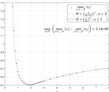
Figure 1. Support radius $R$ of $\mu_{\mathrm{eq}}$ and $\displaystyle\max_{j=1,\ldots,N}|x_{j}|$ for empirical measure with $N=10^{4}$ points, when $d=4$, $s=d-4=0$, and $V=\gamma\left|\cdot\right|^{\alpha}$ with $\gamma=1$ and $\alpha>0$.

A local minimum of a smooth unconstrained function can be found efficiently by a variety of gradient based descent methods, see [25] for example. Here

$$\nabla_{x_{k}}E(\mu_{x_{1},\ldots,x_{N}})=\sum_{\begin{subarray}{c}j=1\\ j\neq k\end{subarray}}^{N}\nabla_{x_{k}}K_{s}(x_{k}-x_{j})+2(N-1)\nabla_{x_{k}}V(x_{k})$$ (1.15)

with $\nabla_{x_{k}}V(x_{k})=\alpha\gamma|x_{k}|^{\alpha-2}\;x_{k}$, and for $k\neq j$,

$$\nabla_{x_{k}}K_{s}(x_{k}-x_{j})=\begin{cases}|s|^{2}\frac{x_{k}-x_{j}}{|x_{k}-x_{j}|^{s+2}}&\text{if $-2<s<0$ or $s>0$}\\ -\frac{x_{k}-x_{j}}{|x_{k}-x_{j}|^{2}}&\text{if $s=0$}\end{cases}.$$ (1.16)

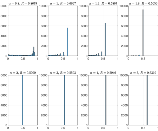
Figure 2. Histograms of point norms $|x_{j}|,j=1,\ldots,N=10^{4}$ of empirical equilibrium measure for $d=4$, $s=d-4=0$, and $V=\gamma\left|\cdot\right|^{\alpha}$ with $\gamma=1$ and selected $\alpha>0$.

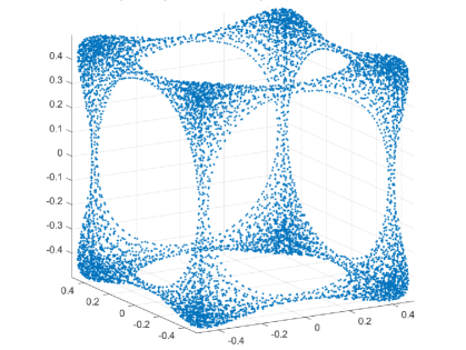
Figure 3. Projection on $x_{1}=0$ of a discrete numerical approximation of the equilibrium measure $\mu_{\mathrm{eq}}$ with $N=10^{4}$ in the case where $s=0$, $d=4$, and $V=\left|\cdot\right|_{4}^{4}$.

The number of optimization variables is $n=dN$ for $N$ points in $\mathbb{R}^{d}$, for example $n=40,000$ for the experiments in Figures 1 and 3, so a limited-memory BFGS method [8] can avoid computations with an $n$ by $n$ Hessian approximation. Gradient information is essential due to the highly nonlinear interactions from the Riesz kernels. For each fixed $N$, there can be many local minima to the discrete optimization problem, thus many different initial points were used to try to identify the global minimum. Furthermore, the external field $V=\gamma\left|\cdot\right|_{p}^{\alpha}$ has a derivative discontinuity at the origin for $p=2$, $\alpha<2$, making discrete optimization for densities with a mass at the origin much more difficult. Also for $p=1$, the external field has derivative discontinuities whenever a component of one of the points is zero.

We further remark that as $N\to\infty$ the sequence of empirical measures $\mu_{N}^{*}:=\mu_{x_{1}^{*},\ldots,x_{N}^{*}}$ for minimizers $\omega_{N}^{*}=(x_{1}^{*},\ldots,x_{N}^{*})$ of the discrete energy in (1.13) converges in the weak-star topology to the corresponding equilibrium measure $\mu_{\mathrm{eq}}$ of Theorem 1.2. Indeed, it is easy to show that thanks to the growth of $V(x)$ at infinity, the empirical measures are all supported on a compact set independent of $N$ and so a standard argument (see for instance Theorem 4.2.2 of [7]) going back to Choquet [13] and Fekete [16] shows that any limit measure of the sequence $\mu_{N}^{*}$ is necessarily an equilibrium (minimizing) measure of the continuous problem in (1.6). Moreover, under the assumptions of Theorem 1.2, this equilibrium measure is unique.

Figures 1 and 2 illustrate the results of some numerical experiments minimizing the modified potential (1.13) using $N=10^{4}$ discrete points $x_{j},j=1,\ldots,N$ for $d=4$, $s=0$, $V=\gamma\left|\cdot\right|^{\alpha}$, $\gamma=1$ and various values for $\alpha$. Figure 1 shows the strong agreement between the empirical support radius $\max_{j=1,\ldots,N}|x_{j}|$ of the discrete measure and the theoretical results in Theorem 1.2. Figure 1 also illustrates the continuity of the support radius at $\alpha=2$, as discussed in Remark 1.3. Figure 2 gives histograms of the discrete measure for various $\alpha$, illustrating the change from $\alpha<2$ when the equilibrium measure is the mixture (1.9) to $\alpha\geq 2$ when the equilibrium measure is the uniform probability density on a sphere of radius $R$ given by (1.12).

2. Remarks and conjectures for general $s$ and $d$

2.1. More general values of $s$ and $d$

We could ask about $\mu_{\mathrm{eq}}$ for more general values of $s$ and $d$. Here are some remarks about a few other cases, beyond the case $d=s+4$ of Theorem 1.2 and the case $d=s+3$ and $\alpha=2$ of [12].

2.1.1. Case $s=d-1$

To the best of our knowledge, little is known when $s=d-1$. However, if $d=1$, $s=d-1=0$ , $V=\left|\cdot\right|^{\alpha}$, $\alpha>0$, and following [26, Th. IV.5.1] (see [21, Pro. 5.3.4] for relation to free probability), then the equilibrium measure $\mu_{\mathrm{eq}}$ is the Ullman distribution on $\mathbb{R}$ with density

$$x\in\mathbb{R}\mapsto\frac{\alpha}{\pi R^{\alpha}}\Bigr{(}\int_{|x|}^{R}\frac{t^{\alpha-1}}{\sqrt{t^{2}-x^{2}}}\mathrm{d}t\Bigr{)}\mathbf{1}_{x\in[-R,R]}\quad\text{where}\quad R:=\left(\frac{\sqrt{\pi}}{\alpha}\frac{\Gamma\bigr{(}\frac{\alpha+2}{2}\bigr{)}}{\Gamma\bigr{(}\frac{\alpha+1}{2}\bigr{)}}\right)^{\frac{1}{\alpha}}.$$ (2.1)

When $\alpha=2$ we recover a semicircle distribution with density $\frac{2}{\pi}\sqrt{1-x^{2}}\mathbf{1}_{x\in[-1,1]}$. Note also that the formula for the radius above has a form similar to the critical radius in the case $s=d-3$ in [12].

When $d-2<s<d$, so that the maximum principle holds, then, one can minimize the Riesz analogue of the Mhaskar – Saff functional (see [26, Chap. IV, eq. (1.1)])

$$\mathcal{F}_{s}(A):=\iint K_{s}(x-y)\mu_{A}(\mathrm{d}x)\mu_{A}(\mathrm{d}y)+\int V(x)\mu_{A}(\mathrm{d}x),$$

where $A$ is a compact set of positive capacity and $\mu_{A}$ is the equilibrium measure for the Riesz minimum $s$-energy problem for $A$ with no external field. Assuming that the support $A$ of $\mu_{\mathrm{eq}}$ is a ball $B_{R}$, for which $\mu_{B_{R}}$ is known, then minimizing $\mathcal{F}_{s}(B_{R})$ leads to the following formula for the radius of the ball

$$R=\left(\frac{|s|\Gamma\bigr{(}\frac{d-s}{2}\bigr{)}\Gamma\bigr{(}\frac{\alpha+2+s}{2}\bigr{)}}{\alpha\Gamma\bigr{(}\frac{\alpha+d}{2}\bigr{)}}\right)^{\frac{1}{\alpha+s}},\,\,\,\,\alpha+s>0.$$ (2.2)

To verify this formula one can use the Frostman conditions (1.8). For $s=d-1$, $d\geq 2$ and $\alpha=2$ the radially symmetric semicircle distribution on the ball $B_{R}$ is, with $y=rR\hat{y}$, $r\in[0,1]$, $\hat{y}\in\mathbb{S}^{d-1}$,

$$\mu_{R}(\mathrm{d}y)=M\sqrt{R^{2}-|y|^{2}}\ \mathbf{1}_{|y|\leq R}\;\mathrm{d}y=MR^{d+1}\sqrt{1-r^{2}}\;r^{d-1}\mathbf{1}_{r\in[0,1]}\,\mathrm{d}r\,\sigma_{1}(\mathrm{d}\hat{y}),$$

where the normalization constant $M$ satisfies

$$M^{-1}=R^{d+1}\int_{0}^{1}\sqrt{1-r^{2}}\,r^{d-1}\mathrm{d}r=R^{d+1}\frac{\sqrt{\pi}}{4}\frac{\Gamma\left(\frac{d}{2}\right)}{\Gamma\left(\frac{d+3}{2}\right)}=\frac{d-1}{d}\frac{\pi}{4}.$$

Also using the parametrization $x=\lambda R\hat{x}$, $\lambda\geq 0$, $\hat{x}\in\mathbb{S}^{d-1}$, and the Funk – Hecke formula of Lemma A.2 for the integral of the Riesz kernel over $\mathbb{S}^{d-1}$, gives

$$U^{\mu_{R}}(x) = \int_{B_{R}}K_{s}(|x-y|)\mu_{R}(\mathrm{d}y)=R^{d-s+1}M\int_{0}^{1}\int_{\mathbb{S}^{d-1}}|\lambda\hat{x}-r\hat{y}|^{-s}\,r^{d-1}\sqrt{1-r^{2}}\;\sigma_{1}(\mathrm{d}\hat{y})\,\mathrm{d}r$$

$$= \frac{R^{2}4d}{(d-1)\pi}\int_{0}^{1}(\lambda+r)^{1-d}{}_{2}F_{1}\left(\frac{d-1}{2},\frac{d-1}{2};d-1;\frac{4\lambda r}{(\lambda+r)^{2}}\right)\,r^{d-1}\sqrt{1-r^{2}}\,\mathrm{d}r.$$

The Frostman conditions for $\mu_{R}$ to be the equilibrium measure are that the modified potential $\varphi(\lambda):=U^{\mu_{R}}(\lambda R\hat{x})+(\lambda R)^{2}$ satisfies $\varphi(\lambda)=c$ for $\lambda\in[0,1]$ and $\varphi(\lambda)>c$ for $\lambda>1$. Here $c=R^{2}\frac{d}{d-1}$ and $\varphi(\lambda)=c$ is equivalent to, for $\lambda\in[0,1]$,

$$\int_{0}^{1}(\lambda+r)^{1-d}{}_{2}F_{1}\left(\frac{d-1}{2},\frac{d-1}{2};d-1;\frac{4\lambda r}{(\lambda+r)^{2}}\right)r^{d-1}\sqrt{1-r^{2}}\;\mathrm{d}r=\frac{\pi}{4}\left(1-\frac{d-1}{d}\lambda^{2}\right),$$ (2.3)

which is [17, Lem. 2.4 with $\alpha=1-d$ and $\ell=1$] divided by $R^{2}|\mathbb{S}^{d-1}|$. Moreover, numerical experiments suggest that the inequality in the Frostman conditions (1.8) holds when $\lambda>1$. It is worth noting that when $d=2$, then (2.3) boils down to the following formula in the same spirit of those in [12]:

$$\int_{0}^{1}K\left(\frac{4\lambda r}{(\lambda+r)^{2}}\right)\frac{r\sqrt{1-r^{2}}}{\lambda+r}\;\mathrm{d}r=\frac{\pi^{2}}{16}\left(2-\lambda^{2}\right),$$ (2.4)

where $K(z)=\dfrac{\pi}{2}\,{}_{2}F_{1}(1/2,1/2;1;z)$ is the complete Elliptic integral of the first kind, (cf. [12, Eq. (1.20)]).

2.1.2. Case $s=d-2$ (Coulomb)

Let us consider the Coulomb case $s=d-2$. From

$$\Delta K_{d-2}=-c_{d}\delta_{0}$$ (2.5)

we get the inversion formula, in the sense of distributions,

$$\Delta U^{\mu}=-c_{d}\mu.$$ (2.6)

When $V$ is locally integrable it can be viewed as a distribution and we get, by combining (1.8) and (2.6), that $\mu_{\mathrm{eq}}$ is equal on the interior of its support, in the sense of distributions, to the distribution

$$\frac{\Delta V}{c_{d}}.$$ (2.7)

Beware that $\mu_{\mathrm{eq}}$ is not necessarily absolutely continuous and may have a singular part outside the interior of its support. In particular, when $V$ is $\mathcal{C}^{2}$ then the interior of the support of $\mu_{\mathrm{eq}}$ does not intersect the set $\{\Delta V<0\}$.

From [23, Prop. 2.13], when $d\geq 3$, $V=\left|\cdot\right|^{\alpha}$, $\alpha>0$ (so $\gamma=1$) the support of the equilibrium measure $\mu_{\mathrm{eq}}$ is a ball of radius $R$, where

$$R=\left(\frac{d-2}{\alpha}\right)^{\frac{1}{d+\alpha-2}}$$ (2.8)

and

$$\mathrm{d}\mu_{\mathrm{eq}}(r\hat{x})=\frac{\alpha(d+\alpha-2)}{d-2}\;r^{d+\alpha-3}\;\mathbf{1}_{0\leq r\leq R}\;\mathrm{d}r\;\sigma_{1}(\mathrm{d}\hat{x}).$$ (2.9)

When $d=2$, so $s=0$, [26, Thm. IV.6.1] shows that

$$R=\left(\frac{1}{\alpha}\right)^{\frac{1}{\alpha}}$$ (2.10)

and

$$\mathrm{d}\mu_{\mathrm{eq}}(r\hat{x})=\alpha^{2}r^{\alpha-1}\;\mathbf{1}_{0\leq r\leq R}\;\mathrm{d}r\;\sigma_{1}(\mathrm{d}\hat{x}).$$ (2.11)

Note that when $\alpha=2$, $\mu_{\mathrm{eq}}$ is uniform on the ball in $\mathbb{R}^{d}$ with volume $c_{d}/(2d)$, which has radius $R$.

2.1.3. Case $s=d-3$

It is proved in [12] that when $d=s+3$ and $V=\gamma\left|\cdot\right|^{2}$, $\gamma>0$, then $\mu_{\mathrm{eq}}$ has a radial arcsine distribution supported on a ball. It is also mentioned in [12] that an explicit computation of $\mu_{\mathrm{eq}}$ is still possible when $V$ belongs to a special class of radial polynomials or hypergeometric functions. On the other hand, when $d=3$, $s=0$, $V=\gamma\left|\cdot\right|^{\alpha}$, $\gamma>0$, it is easily proved that for no value of $\alpha>0$ is the support of $\mu_{\mathrm{eq}}$ a single centered sphere; indeed, it is easy to show that this would violate the Frostman conditions. It is tempting to conjecture that for $d=s+3$, $s\geq 0$, and for any $\alpha>0$, the support of $\mu_{\mathrm{eq}}$ has full dimension. Numerical experiments suggest that when $d=s+3$ then the support of $\mu_{\mathrm{eq}}$ could be a ball when $\alpha\leq 2$ and a shell (region between two concentric spheres) when $\alpha>2$.

2.1.4. Case $s=d-2n$, $n\in\{1,2,3,\ldots\}$, iterated Coulomb

We have the following proposition:

Proposition 2.1 (Iterated Coulomb).

Suppose that $V$ is locally integrable and is such that $\mu_{\mathrm{eq}}$ exists and is characterized by the Frostman conditions (1.8). Then, for $s=d-2n$, the equilibrium measure $\mu_{\mathrm{eq}}$ is equal, on the interior of its support, in the sense of distributions, to the distribution

$$\frac{\Delta^{n}V}{c_{d}C_{d,n}}$$ (2.12)

where $c_{d}$ is defined in (1.2),

$$C_{d,n}:=(-1)^{n-1}\frac{(d-4)!!(2n-2)!!}{(d-2n-2)!!},$$ (2.13)

and $z!!:=\prod_{k=0}^{\lceil\frac{z}{2}\rceil-1}(z-2k)$ is the double factorial (with $z!!:=1$ if $z\leq 0$).
In particular, if $V$ is $\mathcal{C}^{2n}$ on an open set $O\subset\mathbb{R}^{d}$, then

• $O\cap\mathrm{int}(\mathrm{supp}(\mu_{\mathrm{eq}}))\cap\{\Delta^{n}V<0\}=\varnothing$ when $n$ is odd (since then $C_{d,n}>0$);

• $O\cap\mathrm{int}(\mathrm{supp}(\mu_{\mathrm{eq}}))\cap\{\Delta^{n}V>0\}=\varnothing$ when $n$ is even (since then $C_{d,n}<0$).

Before we give a proof of Proposition 2.1, we make the following observations:

• $2n=d-s\leq d+1$ since $s>-2$

• Proposition 2.1 with $n=1$ is the Coulomb case $s=d-2$ of Section 2.1.2

• $\Delta\left|\cdot\right|^{\alpha}=\alpha(\alpha+d-2)\left|\cdot\right|^{\alpha-2}$ which has the same sign as $d+\alpha-2$ (critical value is $\alpha=2-d$)

• Beware that $\mu_{\mathrm{eq}}$ is not necessarily absolutely continuous and can have a singular part supported outside the interior of its support, as shown in Theorem 1.2. Indeed, let us consider the case $d=s+4=s+2n\geq 4$, $n=2$, and $V=\gamma\left|\cdot\right|^{\alpha}$, $\gamma>0$. If $0<\alpha<2,$ then Theorem 1.2 states that $\mu_{\mathrm{eq}}$ is equal, in the sense of distribution, on the interior of its support, to

  $$\beta f=\frac{2-\alpha}{d-2}\frac{\alpha+d-4}{|\mathbb{S}^{d-1}|}\left|\cdot\right|^{\alpha-4}\gamma\frac{\alpha(\alpha+d-2)}{2}\begin{cases}\frac{1}{d-4}&\text{if $d\neq 4$}\\ 1&\text{if $d=4$}\end{cases}.$$

  Alternatively, for $d\geq 3$, $n=2$ (noting that $C_{4,2}=-2,C_{3,2}=2$)

  $$\frac{\Delta^{n}V}{c_{d}C_{d,n}}=\gamma\frac{\Delta^{2}\left|\cdot\right|^{\alpha}}{c_{d}C_{d,2}}=-\gamma\frac{\alpha(\alpha+d-2)(\alpha-2)(\alpha+d-4)}{2(d-2)|\mathbb{S}^{d-1}|}\left|\cdot\right|^{\alpha-4}\begin{cases}\frac{1}{d-4}&\text{if $d\neq 4$}\\ 1&\text{if $d=4$}\end{cases}$$

  which matches the formula for $\beta f$ (including the case $d=3$, $s=-1$ for $1<\alpha<2$)!

  In contrast, if $\alpha\geq 2,$ then

  $$\Delta^{2}V=\gamma\alpha(\alpha+d-2)(\alpha-2)(\alpha+d-4)\left|\cdot\right|^{\alpha-4}>0,$$

  and since $C_{d,2}<0$ we get $\{\Delta^{2}V\geq 0\}=\varnothing$ therefore $\mathrm{int}(\mathrm{supp}(\mu_{\mathrm{eq}}))=\varnothing$, which implies that $\mu_{\mathrm{eq}}$ is singular. Indeed Theorem 1.2 gives in that case $\mu_{\mathrm{eq}}=\sigma_{R}$.

Proof of Proposition 2.1.

For $u>-2$ with $u\neq d-2$, in the sense of distributions,

$$\Delta K_{u}=-c_{d,u}K_{u+2},\quad\text{where}\quad c_{d,u}=\begin{cases}|u|(d-2-u)&\text{if $u\neq 0$}\\ d-2&\text{if $u=0$}\end{cases}.$$ (2.14)

The idea is to apply $\Delta$ repeatedly, $n-1$ times, to pass, via (2.14), by $+2$ steps, from $K_{s}$ to $K_{d-2}$, and then to use (2.5). We know that $\mu_{\mathrm{eq}}$ exists and is unique and satisfies the Euler – Lagrange equations (1.8). Applying $\Delta^{n}$ to both sides of (1.8) gives (see [12, Lemma A.1 (iii)])

$$\Delta^{n}K_{s}*\mu_{\mathrm{eq}}=-\Delta^{n}V\quad\text{on $\mathrm{supp}(\mu_{\mathrm{eq}})$.}$$ (2.15)

If $n>1$, iterating (2.14) and using (2.5) we get, with $C_{d,n}=(-1)^{n-1}\prod_{k=0}^{n-2}c_{d,s+2k}$,

$$\Delta^{n}K_{s}=\Delta(\Delta^{n-1}K_{s})=C_{d,n}\Delta K_{s+2(n-1)}=C_{d,n}\Delta K_{d-2}=-C_{d,n}c_{d}\delta_{0}.$$ (2.16)

Recall that $s=d-2n$. Moreover $C_{d,n}>0$ if $n$ is odd while $C_{d,n}<0$ if $n$ is even. The formula (2.16) remains valid for $n=1$ (namely the Coulomb case $d=s+2$) by taking $C_{d,1}=1$, and reduces then to (2.5). By combining (2.15) and (2.16), we get that $\mu_{\mathrm{eq}}$ is equal to $(C_{d,n}c_{d})^{-1}\Delta^{n}V$ on the interior of $\mathrm{supp}(\mu_{\mathrm{eq}})$. Let us compute the value of $C_{d,n}$ for $n\geq 2$. If $s=d-2n>-2,$ then $d>2$ and

$$(-1)^{n-1}C_{d,n} =\prod_{k=0}^{n-2}c_{d,s+2k}=\prod_{k=0}^{n-2}(s+2k)(d-2-s-2k)$$

$$=\frac{(s+2n-4)!!}{(s-2)!!}\ \frac{(d-s-2)!!}{(d-s-2n)!!}$$

$$=\frac{(d-4)!!}{(d-2n-2)!!}\ (2n-2)!!.$$

Note that this formula also gives $C_{d,1}=1$ for the Coulomb case $n=1$, as desired. ∎

2.2. Different norms

Numerical experiments using different norms, for example $V=\left|\cdot\right|_{p}^{p}$, where $\left|x\right|_{p}^{p}:=|x_{1}|^{p}+\cdots+|x_{d}|^{p}$, give intriguing results, in accordance with (2.12). See for instance Figure 3 for $p=4$. In this case the support of $\mu_{\mathrm{eq}}$ has the symmetries of the $\ell^{p}$ norm but is still a mystery and we do not know if $\mu_{\mathrm{eq}}$ is absolutely continuous, singular, or a mixture of both. Note that the uniform distribution on $\ell^{p}$ balls and spheres in $\mathbb{R}^{d}$ admits remarkable representations and characterizations, see for instance [4, 27]. Another possibility is to modify the kernel, namely to take $\left|\cdot\right|_{p}^{-s}$, and the first question is then the positive definiteness in order to get convexity and uniqueness of $\mu_{\mathrm{eq}}$.

In $\mathbb{R}^{d}$ with $d=2n$, when $V=\left|\cdot\right|_{2n}^{2n}$, the support of $\mu_{\mathrm{eq}}$ has the symmetries of $\left|\cdot\right|_{2n}$ (spherical when $n=1$). Furthermore, since $\Delta^{n}V=(2n)!d$ is a non-zero constant, we get from (2.12) that if $n$ is odd, then $\mu_{\mathrm{eq}}$ is uniform (constant density) on the interior of its support, while if $n$ is even then the interior of the support of $\mu_{\mathrm{eq}}$ is empty and $\mu_{\mathrm{eq}}$ is singular. If $n=1$, then $\Delta^{n}V$ is constant (Coulomb case) and $\mu_{\mathrm{eq}}$ is the uniform law on a ball.

3. Proof of Theorem 1.2

We first consider the equilibrium problem restricted to spheres (Section 3.1). This spherical case is essential for the proof of the case $\alpha\geq 2$ which is given in Section 3.2. We then provide the proof of the case $d\geq 4$ and $1<\alpha<2$ (Section 3.3), and then the proof of the case $d=3$ (Section 3.4). As in the statement of Theorem 1.2, we have to consider separately the cases $d=3$ ($s=-1$), $d=4$ ($s=0$), and $d>4$ ($s>0$), which is done respectively in Lemmas 3.4, 3.6, and 3.7.

3.1. Optimal spheres

We first consider the equilibrium problem restricted to spheres and provide some simple lemmas that are needed in the proof of part (i)(b) of assertion ($i$) of Theorem 1.2.

Throughout this section, $V=\gamma\left|\cdot\right|^{\alpha}$, $\gamma>0$, $\alpha>0$, and we use of the fact that for $R>0$, $K_{s}*\sigma_{R}+V$ is radially symmetric, and so for $x\in\mathbb{R}^{d}$, we introduce the parametrization $x=\lambda R\hat{x}$ with $\lambda\geq 0$ and $|\hat{x}|=1$, and we only need to consider

$$\varphi(\lambda)=\varphi_{\sigma_{R}}(\lambda):=(K_{s}*\sigma_{R}+V)(\lambda R\hat{x}),\quad\lambda\geq 0,\quad\hat{x}\in\mathbb{S}^{d-1}.$$ (3.1)

Note that with this parametrization, the critical value for $\lambda$ is $\lambda=1$, regardless of the value of $R$.

Lemma 3.1.

Let $d\geq 2$, $s>-2$ and $\varphi$ be as in (3.1). Then, with the above notation, for $x\in\mathbb{R}^{d}$, and with $\tau_{d-1}$ as in Lemma A.2, we have

$$\varphi(\lambda)=\begin{cases}\displaystyle\frac{\tau_{d-1}}{R^{s}}\int_{-1}^{1}\frac{(1-t^{2})^{\frac{d-3}{2}}}{(\lambda^{2}+1-2\lambda t)^{\frac{s}{2}}}\mathrm{d}t+\gamma(\lambda R)^{\alpha}&\text{if $s\neq 0$}\\[10.00002pt] \displaystyle-\log R-\frac{\tau_{d-1}}{2}\int_{-1}^{1}\log(\lambda^{2}+1-2\lambda t)(1-t^{2})^{\frac{d-3}{2}}\mathrm{d}t+\gamma(\lambda R)^{\alpha}&\text{if $s=0$}\end{cases}.$$

Moreover $\varphi$ is continuous on $[0,\infty)$ and differentiable on $(0,+\infty)$, and for $\lambda>0$,

$$\varphi^{\prime}(\lambda)=\begin{cases}\displaystyle\frac{s\tau_{d-1}}{R^{s}}\int_{-1}^{1}\frac{(t-\lambda)(1-t^{2})^{\frac{d-3}{2}}}{(\lambda^{2}+1-2\lambda t)^{\frac{s+2}{2}}}\mathrm{d}t+\gamma\alpha R^{\alpha}\lambda^{\alpha-1}&\text{if $s\neq 0$}\\[10.00002pt] \displaystyle\tau_{d-1}\int_{-1}^{1}\frac{(t-\lambda)(1-t^{2})^{\frac{d-3}{2}}}{\lambda^{2}+1-2\lambda t}\mathrm{d}t+\gamma\alpha R^{\alpha}\lambda^{\alpha-1}&\text{if $s=0$}\end{cases}.$$

Proof.

The result follows from the identity

$$\int_{\mathbb{S}^{d-1}_{R}}K_{s}(x-y)\sigma_{R}(\mathrm{d}y)=\begin{cases}\displaystyle R^{-s}\int_{\mathbb{S}^{d-1}}(\lambda^{2}-2\lambda\hat{x}\cdot\hat{y}+1)^{-\frac{s}{2}}\sigma_{1}(\mathrm{d}\hat{y})&\text{if $s\neq 0$}\\[10.00002pt] \displaystyle-\log R-\frac{1}{2}\int_{\mathbb{S}^{d-1}}\log(\lambda^{2}-2\lambda\hat{x}\cdot\hat{y}+1)\sigma_{1}(\mathrm{d}\hat{y})&\text{if $s=0$}\end{cases},$$

which holds for arbitrary $\hat{x}\in\mathbb{S}^{d-1}$, and the Funk – Hecke formula of Lemma A.2. ∎

Lemma 3.2.

Assume that

$$d\geq 3,\quad-2<s\leq d-4,\quad V=\gamma\left|\cdot\right|^{\alpha},\ \alpha\geq 2.$$

The energy function $\eta(R):=\mathrm{I}(\sigma_{R})$, from (1.5), achieves its infimum on $(0,\infty)$ at the unique point

$$R:=\begin{cases}\left(\frac{sW_{s,d-1}}{2\gamma\alpha}\right)^{\frac{1}{s+\alpha}}&\text{if $s\neq 0$}\\ \left(\frac{1}{2\gamma\alpha}\right)^{\frac{1}{\alpha}}&\text{if $s=0$}\end{cases},$$

where $W_{s,d-1}$ is the Wiener constant for $\mathbb{S}^{d-1}$ given by

$$W_{s,d-1}:=\iint K_{s}(x-y)\sigma_{1}(\mathrm{d}x)\sigma_{1}(\mathrm{d}y)=\begin{cases}\displaystyle\mathrm{sign}(s)\frac{\Gamma(\frac{d}{2})\Gamma(d-1-s)}{\Gamma(\frac{d-s}{2})\Gamma(d-1-\frac{s}{2})}&\text{if $-2<s<0$, or}\\[-4.30554pt] &\text{if $0<s<d-1$ and $d\geq 4$}\\[10.00002pt] \displaystyle-\log(2)+\frac{\psi(d-1)-\psi(\frac{d-1}{2})}{2}&\text{if $s=0$ and $d\geq 4$}\end{cases},$$

and $\psi(z):=\Gamma^{\prime}(z)/\Gamma(z)$ is the digamma special function, see for example [7, Prop. 4.6.4, p. 180].

Note that $-2<s\leq d-4$ implies $d>2$; hence $d\geq 3$.

We also remark that when $s=0$, the radius $R$ does not depend on the dimension $d$.

Proof.

We have

$$\eta(R):=\mathrm{I}(\mu_{R}) =\iint_{\mathbb{S}^{d-1}_{R}\times\mathbb{S}^{d-1}_{R}}K_{s}(x-y)\sigma_{R}(\mathrm{d}x)\sigma_{R}(\mathrm{d}y)+2\int_{\mathbb{S}^{d-1}_{R}}V(x)\sigma_{R}(\mathrm{d}x)$$

$$=\iint_{\mathbb{S}^{d-1}\times\mathbb{S}^{d-1}}K_{s}(R\hat{x}-R\hat{y})\sigma_{1}(\mathrm{d}\hat{x})\sigma_{1}(\mathrm{d}\hat{y})+2\gamma R^{\alpha}.$$

Case $s=0$. In this case, we have $K_{s}(x-y)=K_{0}(R(\hat{x}-\hat{y}))=-\log(R)-\log|\hat{x}-\hat{y}|$, and thus

$$\eta(R)=-\log(R)-\iint_{\mathbb{S}^{d-1}\times\mathbb{S}^{d-1}}\log|\hat{x}-\hat{y}|\sigma_{1}(\mathrm{d}\hat{x})\sigma_{1}(\mathrm{d}\hat{y})+2\gamma R^{\alpha}.$$

Now $\eta$ is strictly convex and reaches its minimum at the unique optimal point

$$R_{*}=\left(\frac{1}{2\gamma\alpha}\right)^{1/\alpha}.$$ (3.2)

Case $-2<s<d-4$, $s\neq 0$.

$$\eta(R)=\frac{W_{s,d-1}}{R^{s}}+2\gamma R^{\alpha}\quad\mbox{where}\quad W_{s,d-1}=\iint_{\mathbb{S}^{d-1}\times\mathbb{S}^{d-1}}K_{s}(\hat{x}-\hat{y})\sigma_{1}(\mathrm{d}\hat{x})\sigma_{1}(\mathrm{d}\hat{y}).$$

The equation $\eta^{\prime}(R)=0$ has a unique solution (critical point) given by

$$R_{*}=\left(\frac{sW_{s,d-1}}{2\gamma\alpha}\right)^{1/(s+\alpha)}.$$ (3.3)

We have

$$\eta^{\prime\prime}(R) =s(s+1)R^{-(s+2)}W_{s,d-1}+2\gamma\alpha(\alpha-1)R^{\alpha-2}$$

$$=R^{-(s+2)}\left(s(s+1)W_{s,d-1}+2\gamma\alpha(\alpha-1)R^{\alpha+s}\right),$$

and thus

$$\eta^{\prime\prime}(R_{*})=\left(\frac{2\gamma\alpha}{sW_{s,d-1}}\right)^{\frac{s+2}{\alpha+s}}s(s+\alpha)W_{s,d-1}.$$

It follows that $\eta^{\prime\prime}(R_{*})>0$ since $s+\alpha>0$ and since $s$ and $W_{s,d-1}$ have the same sign. ∎

3.2. Case $\alpha\geq 2$

Let $V=\gamma\left|\cdot\right|^{\alpha}$ with $\gamma>0$ and $\alpha\geq 2$. We have to show that $\mu_{\mathrm{eq}}$ is uniform on a sphere. For this purpose, we verify the Frostman conditions (1.8) which asserts that the support of $\mu_{\mathrm{eq}}$ is a sphere of radius $R$ if and only if, for some constant $c$, we have $\varphi(\lambda)=c$ when $\lambda=1$ and $\varphi(\lambda)>c$ when $\lambda\neq 1$. Since $\varphi$ is continuous on $[0,+\infty)$ and differentiable on $(0,+\infty)$, part (i)-(i)(b) of Theorem 1.2 follows from Lemma 3.3 in the case where $s=0$ and $d\geq 4$, part (ii)-(ii)(c) from Lemma 3.4 in the case where $s=-1$ and $d=3$, and Lemma 3.7 in the case $d\geq 5$ and $s=d-4$.

Lemma 3.3.

Let $\varphi$ be as in (3.1) with $s=0$, $d\geq 4$, $\alpha\geq 2$, and $R=(\frac{1}{2\gamma\alpha})^{\frac{1}{\alpha}}$. Then

$$\varphi^{\prime}(\lambda)=\frac{1}{2\lambda}\left[\frac{1-\lambda^{2}}{1+\lambda^{2}}\ {}_{2}F_{1}\left(\frac{1}{2},1;\frac{d}{2};\frac{4\lambda^{2}}{(1+\lambda^{2})^{2}}\right)-1\right]+\frac{\lambda^{\alpha-1}}{2},\quad\lambda>0.$$

Moreover $\varphi^{\prime}(\lambda)<0$ if $0<\lambda<1$, $\varphi^{\prime}(1)=0$, while $\varphi^{\prime}(\lambda)>0$ if $\lambda>1$.

Proof.

In view of the formula given by Lemma 3.1, we have, with $\zeta:=4\lambda^{2}/(1+\lambda^{2})^{2}$,

$$J :=\int_{-1}^{1}\frac{(t-\lambda)(1-t^{2})^{\frac{d-3}{2}}}{\lambda^{2}+1-2\lambda t}\mathrm{d}t$$

$$=\frac{\zeta}{4\lambda}\int_{0}^{1}\frac{2t^{2}-(1+\lambda^{2})}{1-\zeta t^{2}}(1-t^{2})^{\frac{d-3}{2}}\mathrm{d}t$$

$$=\frac{\zeta}{4\lambda}\int_{0}^{1}\frac{2u^{1/2}-u^{-1/2}(1+\lambda^{2})}{1-\zeta u}(1-u)^{\frac{d-3}{2}}\mathrm{d}u.$$

The Euler integral representation of Lemma A.1 gives in particular, for $a>-1$, $b>-1$, $|\zeta|<1$,

$$\int_{0}^{1}\frac{u^{a-1}(1-u)^{b-1}}{1-\zeta u}\mathrm{d}u=\frac{\Gamma(a)\Gamma(b)}{\Gamma(a+b)}\ {}_{2}F_{1}(a,1;a+b;\zeta).$$

Using this formula with $a\in\{3/2,1/2\}$, $b=(d-1)/2$, $c=1$, and $\Gamma(\zeta+1)=\zeta\Gamma(\zeta)$, we get

$$\tau_{d-1}J=\frac{\zeta}{4\lambda}\left[\frac{2}{d}\ {}_{2}F_{1}\left(\frac{3}{2},1;\frac{d+2}{2};\zeta\right)-(1+\lambda^{2})\ {}_{2}F_{1}\left(\frac{1}{2},1;\frac{d}{2};\zeta\right)\right].$$

At this step, we observe that the identity $\zeta(\zeta+1)_{k}=(\zeta)_{k+1}$ gives the formula

$$1+\frac{a}{b}\zeta\ {}_{2}F_{1}(a+1,1;b+1;\zeta)={}_{2}F_{1}(a,1;b;\zeta).$$

Finally, using this formula, we obtain, denoting $G:={}_{2}F_{1}\left(\frac{1}{2},1;\frac{d}{2},\zeta\right):=\sum_{k=0}^{\infty}\frac{(\frac{1}{2})_{k}}{(\frac{d}{2})_{k}}\zeta^{k}$,

$$\tau_{d-1}J=\frac{\zeta}{4\lambda}\left[\frac{2}{\zeta}(G-1)-(1+\lambda^{2})G\right]=\frac{1}{2\lambda}\left[\frac{1-\lambda^{2}}{1+\lambda^{2}}G-1\right].$$

Hence the formula for $\varphi^{\prime}(\lambda)$. Alternatively, we could also use the formula for $\varphi$ of Lemma 3.1 to get

$$\varphi(\lambda)=\frac{\log(2\gamma\alpha)}{\alpha}+\frac{\lambda^{2}}{d(1+\lambda^{2})^{2}}\ {}_{3}F_{2}\left(1,1,\frac{3}{2};2,\frac{d+2}{2};\frac{4\lambda^{2}}{(1+\lambda^{2})^{2}}\right)-\frac{\log(1+\lambda^{2})}{2}+\frac{\lambda^{\alpha}}{2\alpha}.$$ (3.4)

At this step, we observe that the formula in the statement of the lemma for $\varphi^{\prime}$ gives $\varphi^{\prime}(1)=0$ as the parameters of the ${}_{3}F_{2}$ function ensure that it is finite (see Lemma A.1 or [14, eqn. 15.4.20]). It remains to determine the sign of $\varphi^{\prime}(\lambda)$ for $\lambda\neq 1$. Let us consider first the case $d=4$. As

$${}_{2}F_{1}\left(\frac{1}{2},1;2;\zeta\right)=\sum_{k=0}^{\infty}\frac{(\frac{1}{2})_{k}}{(k+1)!}\zeta^{k}=2\frac{1-\sqrt{1-\zeta}}{\zeta},$$ (3.5)

we get

$${}_{2}F_{1}\left(\frac{1}{2},1;2;\zeta\right)=\begin{cases}\displaystyle 1+\lambda^{2}&\text{if $0\leq\lambda\leq 1$}\\[2.5pt] \displaystyle 1+\frac{1}{\lambda^{2}}&\text{if $\lambda\geq 1$}\end{cases},$$

and therefore

$$\varphi^{\prime}(\lambda)=\begin{cases}\displaystyle-\frac{\lambda}{2}+\frac{\lambda^{\alpha-1}}{2}&\text{if $0\leq\lambda\leq 1$}\\[5.0pt] \displaystyle\frac{1-2\lambda^{2}}{2\lambda^{3}}+\frac{\lambda^{\alpha-1}}{2}&\text{if $\lambda\geq 1$}\end{cases}.$$

Alternatively, we could use Lemma 3.6 which replaces the Taylor series expansion behind the hypergeometric based formulas by the generating series of orthogonal polynomials. From this it can be checked that $\varphi^{\prime}(\lambda)<0$ if $0<\lambda<1$ while $\varphi^{\prime}(\lambda)>0$ if $\lambda>1$, first when $\alpha=2$ and then by monotony for all $\alpha\geq 2$. This proves the desired result for $d=4$. For the general case $d\geq 4$, noting that ${}_{2}F_{1}\left(\frac{1}{2},1;\frac{d}{2};z\right)$, $z\in[0,1]$, decreases as $d$ increases, an examination of the formula for $\varphi^{\prime}(\lambda)$ reveals that as $d$ increases, then $\varphi^{\prime}(\lambda)$ decreases when $0<\lambda<1$, while $\varphi^{\prime}(\lambda)$ increases when $\lambda>1$, which reduces the analysis to the case $d=4$. ∎

Lemma 3.4.

Let $\varphi$ be as in (3.1), $(d,s)=(3,-1)$, $\alpha\geq 2$, and $R=(\frac{2}{3\gamma\alpha})^{\frac{1}{\alpha-1}}$. Then

$$\varphi^{\prime}(\lambda) =R\begin{cases}-\frac{2}{3}\lambda+\frac{2}{3}\lambda^{\alpha-1}&\text{if $0<\lambda\leq 1$}\\ -1+\frac{1}{3\lambda^{2}}+\frac{2}{3}\lambda^{\alpha-1}&\text{if $\lambda>1$}\end{cases}.$$

Moreover $\varphi^{\prime}(\lambda)\leq 0$ if $0<\lambda<1$, $\varphi^{\prime}(1)=0$, while $\varphi^{\prime}(\lambda)>0$ if $\lambda>1$.

Proof.

From Lemma 3.1 we get, for $\lambda\geq 0$,

$$\varphi(\lambda) =-\frac{R}{2}\int_{-1}^{1}(\lambda^{2}-2\lambda t+1)^{1/2}\mathrm{d}t+\gamma(\lambda R)^{\alpha}$$

$$=-R\frac{|\lambda-1|^{3}-(\lambda+1)^{3}}{6\lambda}+\gamma(\lambda R)^{\alpha}$$

$$=R\begin{cases}-(1+\frac{\lambda^{2}}{3})+\gamma\lambda^{\alpha}R^{\alpha-1}&\text{if $0\leq\lambda\leq 1$}\\ -(\lambda+\frac{1}{3\lambda})+\gamma\lambda^{\alpha}R^{\alpha-1}&\text{if $\lambda>1$}\end{cases}.$$

Hence

$$\varphi^{\prime}(\lambda)=R\begin{cases}-\frac{2}{3}\lambda+\gamma\alpha(\lambda R)^{\alpha-1}&\text{if $0<\lambda\leq 1$}\\ -1+\frac{1}{3\lambda^{2}}+\gamma\alpha(\lambda R)^{\alpha-1}&\text{if $\lambda>1$}\end{cases}.$$

From now on we take $R=(\frac{2}{3\gamma\alpha})^{\frac{1}{\alpha-1}}$, which makes the critical value of $\lambda$ on $(0,1]$ equal to $1$. Hence

$$\varphi^{\prime}(\lambda)=R\begin{cases}-\frac{2}{3}\lambda+\frac{2}{3}\lambda^{\alpha-1}&\text{if $0<\lambda\leq 1$}\\ -1+\frac{1}{3\lambda^{2}}+\frac{2}{3}\lambda^{\alpha-1}&\text{if $\lambda>1$}\end{cases}.$$

Now $\varphi^{\prime}(1)=0$, and moreover $\varphi^{\prime}(\lambda)<0$ for $0<\lambda<1$ when $\alpha>2$ while $\varphi^{\prime}(\lambda)=0$ for $0<\lambda<1$ when $\alpha=2$. If $\lambda>1$, then $(\lambda^{2}\varphi^{\prime}(\lambda))^{\prime}=R(-2\lambda+\frac{2}{3}(\alpha+1)\lambda^{\alpha})>0$ when $\lambda>(3/(1+\alpha))^{1/(\alpha-1)}$, and this last value is $\leq 1$ since $\alpha\geq 2$, which implies that $\varphi^{\prime}(\lambda)>0$ for $\lambda>1$. ∎

Remark 3.5 (General $s$).

Suppose that $s>-2$, $s\neq 0$, and $d\geq 4$. By proceeding as in the proof of Lemma 3.3, it is possible to obtain the following formulas, for all $\lambda\geq 0$,

$$\tau_{d-1}\int_{-1}^{1}\frac{(1-t^{2})^{\frac{d-3}{2}}}{(\lambda^{2}+1-2\lambda t)^{\frac{s}{2}}}\mathrm{d}t=(1+\lambda^{2})^{-\frac{s}{2}}\ {}_{2}F_{1}\left(\frac{s}{4},\frac{s+2}{4};\frac{d}{2};\frac{4\lambda^{2}}{(1+\lambda^{2})^{2}}\right)$$

and

$$\tau_{d-1}\int_{-1}^{1}\frac{(t-\lambda)(1-t^{2})^{\frac{d-3}{2}}}{(\lambda^{2}+1-2\lambda t)^{\frac{s+2}{2}}}\mathrm{d}t\\ =\frac{\lambda}{d(1+\lambda^{2})^{\frac{s+4}{2}}}\Bigg{[}-\frac{(1+\lambda^{2})}{d}\ {}_{2}F_{1}\left(\frac{s+2}{4},\frac{s+4}{4};\frac{d}{2};\frac{4\lambda^{2}}{(1+\lambda^{2})^{2}}\right)\\ +(2+s)\ {}_{2}F_{1}\left(\frac{s+2}{4}+1,\frac{s+4}{4};\frac{d}{2}+1;\frac{4\lambda^{2}}{(1+\lambda^{2})^{2}}\right)\Bigg{]}.$$

This gives formulas for $\varphi(\lambda)$ and $\varphi^{\prime}(\lambda)$ via Lemma 3.1. Unfortunately, the formula for $\varphi^{\prime}(\lambda)$ does not seem to be monotonic with respect to $d$, and thus one cannot proceed as in proof of Lemma 3.3.

When $s$ is an integer, instead of using power series and hypergeometric functions for the evaluation of the integrals in the formulas for $\varphi$ and $\varphi^{\prime}$ of Lemma 3.1, we could use alternatively orthogonal polynomials, which leads for instance when $s=0$ to the trigonometric formulas of Lemma 3.6.

Lemma 3.6 (Trigonometric formulas).

Let $\varphi$ be as in (3.1) with $s=0$, $d=4+2m$ where $m$ is a non-negative integer, and $R=(\frac{1}{2\gamma\alpha})^{\frac{1}{\alpha}}$. Then

$$\varphi^{\prime}(\lambda)=\begin{cases}\displaystyle\frac{\tau_{2m+3}}{2}\sum_{n=0}^{m}\lambda^{2n+1}\int_{0}^{\pi}\sin(\theta)^{2m+1}(\sin((2n+3)\theta)-\sin((2n+1)\theta))\mathrm{d}\theta+\frac{\lambda^{\alpha-1}}{2}&\text{if $0\leq\lambda\leq 1$}\\[10.00002pt] \displaystyle\frac{\tau_{2m+3}}{2}\sum_{n=0}^{m}\frac{1}{\lambda^{2n+3}}\int_{0}^{\pi}\sin(\theta)^{2m+1}(\sin((2n+3)\theta)-\sin((2n+1)\theta)(2\lambda^{2}-1))\mathrm{d}\theta+\frac{\lambda^{\alpha-1}}{2}&\text{if $\lambda\geq 1$}\end{cases},$$

where $\tau$ is as in Lemma A.2. In particular, when $d=4$ ($m=0$), we find

$$\varphi^{\prime}(\lambda)=\begin{cases}\displaystyle-\frac{\lambda}{2}+\frac{\lambda^{\alpha-1}}{2}&\text{if $0\leq\lambda\leq 1$}\\[5.0pt] \displaystyle\frac{1-2\lambda^{2}}{2\lambda^{3}}+\frac{\lambda^{\alpha-1}}{2}&\text{if $\lambda\geq 1$}\end{cases},$$

while when $d=6$ ($m=1$), we find

$$\varphi^{\prime}(\lambda)=\begin{cases}\displaystyle-\frac{2\lambda}{3}+\frac{\lambda^{3}}{6}+\frac{\lambda^{\alpha-1}}{2}&\text{if $0\leq\lambda\leq 1$}\\[5.0pt] \displaystyle\frac{-1+4\lambda^{2}-6\lambda^{4}}{6\lambda^{5}}+\frac{\lambda^{\alpha-1}}{2}&\text{if $\lambda\geq 1$}\end{cases}.$$

Proof.

In view of Lemma 3.1, it suffices to compute

$$I(\lambda):=\int_{-1}^{1}\frac{t-\lambda}{\lambda^{2}+1-2\lambda t}(1-t^{2})^{\frac{d-3}{2}}\mathrm{d}t.$$

Let ${(U_{n})}_{n\geq 0}$ be the Chebyshev orthogonal polynomials of the second kind, orthogonal with respect to the semicircle weight $t\mapsto\sqrt{1-t^{2}}$ on $[-1,1]$. In order to compute $I(\lambda)$, the idea is to exploit their generating series formula, which states, for $|t|<1$ and $|\lambda|<1$,

$$\frac{1}{1+\lambda^{2}-2\lambda t}=\sum_{n=0}^{\infty}U_{n}(t)\lambda^{n}.$$

The orthogonality relation states, for all polynomial $P$ of degree $k\geq 0$ and all $n>k$,

$$\int_{-1}^{1}P(t)U_{n}(t)\sqrt{1-t^{2}}\,\mathrm{d}t=0.$$

Now, since $m:=\frac{d-4}{2}$ is a non-negative integer, the expression $(t-\lambda)(1-t^{2})^{m}$ is a polynomial of degree $k=2m+1$ with respect to $t$, and therefore, when $|\lambda|<1$,

$$I(\lambda)=\sum_{n=0}^{2m+1}\lambda^{n}\int_{-1}^{1}(t-\lambda)(1-t^{2})^{m}U_{n}(t)\sqrt{1-t^{2}}\,\mathrm{d}t,$$

where we have used crucially the identity $(1-t^{2})^{\frac{d-3}{2}}=(1-t^{2})^{m}\sqrt{1-t^{2}}$. Now, to evaluate the integral in the right-hand side above, we use the trigonometric change of variable $t=\cos(\theta)$ and the fact that $U_{n}(\cos(\theta))=\sin((n+1)\theta)/\sin(\theta)$, which give

$$\int_{-1}^{1}(t-\lambda)(1-t^{2})^{m}U_{n}(t)\sqrt{1-t^{2}}\,\mathrm{d}t=\int_{0}^{\pi}(\cos(\theta)-\lambda)\sin(\theta)^{2m+1}\sin((n+1)\theta)\mathrm{d}\theta.$$

It follows that if $0<\lambda<1$, then using standard trigonometric formulas,

$$I(\lambda)=\frac{1}{2}\sum_{n=0}^{m}\lambda^{2n+1}\int_{0}^{\pi}\sin(\theta)^{2m+1}(\sin((2n+3)\theta)-\sin((2n+1)\theta))\mathrm{d}\theta.$$

This produces the desired formula for $\varphi^{\prime}(\lambda)$ when $0<\lambda<1$.

Let us establish now the formula when $\lambda>1$. Let us set $\rho:=1/\lambda$. Then we have

$$I(\lambda)=\rho^{2}I(\rho)+\rho(\rho^{2}-1)\int_{-1}^{1}\frac{(1-t^{2})^{\frac{d-3}{2}}}{1+\rho^{2}-2\rho t}\mathrm{d}t.$$

Since $0<\rho<1$, proceeding as before for $I(\rho)$, we get for the last integral

$$\int_{-1}^{1}\frac{(1-t^{2})^{\frac{d-3}{2}}}{1+\rho^{2}-2\rho t}\mathrm{d}t =\sum_{n=0}^{m}\rho^{2n}\int_{0}^{\pi}\sin(\theta)^{2m+1}\sin((2n+1)\theta)\mathrm{d}\theta$$

where the last step comes from symmetry of $\sin$. Hence the desired formulas for $\varphi^{\prime}(\lambda)$. ∎

Lemma 3.7.

Let $\varphi$ be as in (3.1) with $d\geq 5$, $s=d-4$, $\alpha\geq 2$, and $R$ as in Theorem 1.2. Then

$$\varphi^{\prime}(\lambda)=\begin{cases}\displaystyle\frac{2s}{(s+4)R^{s}}(-\lambda+\lambda^{\alpha-1})&\text{if $0\leq\lambda\leq 1$}\\[10.00002pt] \displaystyle\frac{s}{(s+4)R^{s}}\Bigr{(}\frac{2-(s+4)+(s+4)\lambda^{2}+2\lambda^{s+\alpha+2}}{\lambda^{s+3}}\Bigr{)}&\text{if $\lambda\geq 1$}\end{cases}.$$

Moreover $\varphi^{\prime}(\lambda)<0$ if $0<\lambda<1$, $\varphi^{\prime}(1)=0$, while $\varphi^{\prime}(\lambda)>0$ if $\lambda>1$.

Proof.

From Lemma 3.1 we get

$$\varphi^{\prime}(\lambda)=-\frac{s\tau_{s+3}}{R^{s}}\int_{-1}^{1}\frac{(\lambda-t)(1-t^{2})^{\frac{s+1}{2}}}{(\lambda^{2}+1-2\lambda t)^{\frac{s+2}{2}}}\mathrm{d}t+\gamma\alpha R^{\alpha}\lambda^{\alpha-1}.$$

The idea is to imitate the proof of Lemma 3.6, and compute $\varphi^{\prime}(\lambda)$ using the following generating series, valid for all $|t|<1$ and $|\lambda|<1$,

$$\frac{1}{(1+\lambda^{2}-2\lambda t)^{\ell}}=\sum_{n=0}^{\infty}C^{(\ell)}_{n}(t)\lambda^{n}$$

where $(C^{(\ell)}_{n})_{n\geq 0}$ are the Gegenbauer ultraspherical polynomials of parameter $\ell:=\frac{s+2}{2}$, orthogonal on $[-1,1]$ with respect to the measure $\mathrm{d}\mu(t)=(1-t^{2})^{\ell-\frac{1}{2}}\mathrm{d}t=(1-t^{2})^{\frac{s+1}{2}}\mathrm{d}t$. The choice of $\ell$ is dictated by the formula for $\varphi^{\prime}(\lambda)$ above. Using $C_{0}^{(\ell)}=1$, $C_{1}^{(\ell)}(t)=(s+2)t$ and orthogonality gives

$$\int_{-1}^{1}\frac{(\lambda-t)(1-t^{2})^{\frac{s+1}{2}}}{(\lambda^{2}+1-2\lambda t)^{\frac{s+2}{2}}}\mathrm{d}t =\sum_{n=0}^{\infty}\lambda^{n}\int_{-1}^{1}(\lambda-t)C_{n}^{(\ell)}(t)\mathrm{d}\mu(t)$$

$$=\lambda\int_{-1}^{1}(1-t^{2})^{\frac{s+1}{2}}\mathrm{d}t-\lambda\int_{-1}^{1}tC_{1}^{(\ell)}(t)\mathrm{d}\mu(t)$$

$$=\frac{\lambda}{\tau_{s+3}}-\lambda(s+2)\int_{-1}^{1}t^{2}(1-t^{2})^{\frac{s+1}{2}}\mathrm{d}t$$

$$=\frac{\lambda}{\tau_{s+3}}-\lambda(s+2)\frac{\Gamma(3/2)\Gamma((s+3)/2)}{\Gamma(3+s/2)}$$

$$=\frac{2\lambda}{(s+4)\tau_{s+3}}.$$

Hence, for $0<\lambda<1$, we obtain

$$\varphi^{\prime}(\lambda)=-\frac{2s}{(s+4)R^{s}}\lambda+\gamma\alpha R^{\alpha}\lambda^{\alpha-1}=\frac{2s}{(s+4)R^{s}}\Bigr{(}-\lambda+\gamma\alpha\frac{s+4}{2s}R^{s+\alpha}\lambda^{\alpha-1}\Bigr{)}$$

which leads to the desired formula when we take $R=(\frac{2s}{(s+4)\gamma\alpha})^{\frac{1}{s+\alpha}}$.

Let us consider now the case $\lambda>1$. Denoting $\rho:=1/\lambda$, we have

$$\int_{-1}^{1}\frac{(\lambda-t)(1-t^{2})^{\frac{s+1}{2}}}{(\lambda^{2}+1-2\lambda t)^{\frac{s+2}{2}}}\mathrm{d}t=\rho^{s+2}\int_{-1}^{1}\frac{(\rho-t)(1-t^{2})^{\frac{s+1}{2}}}{(1+\rho^{2}-2\rho t)^{\frac{s+2}{2}}}\mathrm{d}t+\rho^{s+1}(1-\rho^{2})\int_{-1}^{1}\frac{(1-t^{2})^{\frac{s+1}{2}}}{(1+\rho^{2}-2\rho t)^{\frac{s+2}{2}}}\mathrm{d}t.$$

Now, using the fact that $0<\rho<1$, we get, from the previous computations,

$$\int_{-1}^{1}\frac{(1-t^{2})^{\frac{s+1}{2}}}{(1+\rho^{2}-2\rho t)^{\frac{s+2}{2}}}\mathrm{d}t=\int_{-1}^{1}(1-t^{2})^{\frac{s+1}{2}}\mathrm{d}t=\int_{0}^{1}u^{-1/2}(1-u)^{\frac{s+1}{2}}\mathrm{d}u=\frac{1}{\tau_{s+3}}$$

and

$$\varphi^{\prime}(\lambda) =-\frac{s}{R^{s}}\Bigr{(}\frac{2}{(s+4)\lambda^{s+3}}-\frac{1}{\lambda^{s+3}}+\frac{1}{\lambda^{s+1}}\Bigr{)}+\gamma\alpha R^{\alpha}\lambda^{\alpha-1}$$

$$=\frac{2s}{(s+4)R^{s}}\Bigr{(}\frac{2-(s+4)+(s+4)\lambda^{2}}{2\lambda^{s+3}}+\gamma\alpha\frac{s+4}{2s}R^{s+\alpha}\lambda^{\alpha-1}\Bigr{)}.$$

Hence with $R=(\frac{2s}{(s+4)\gamma\alpha})^{\frac{1}{s+\alpha}}$ we find, for $\lambda>1$,

$$\varphi^{\prime}(\lambda)=\frac{s}{(s+4)R^{s}}\Bigr{(}\frac{2-(s+4)+(s+4)\lambda^{2}+2\lambda^{s+\alpha+2}}{\lambda^{s+3}}\Bigr{)}.$$

The method works more generally when $m:=(d-4-s)/2$ is a non-negative integer, by using $(1-t^{2})^{\frac{d-3}{2}}=(1-t^{2})^{\frac{d-4-s}{2}}(1-t^{2})^{\frac{s+1}{2}}$ where $(1-t^{2})^{\frac{d-4-s}{2}}=(1-t^{2})^{m}$ is then a polynomial in $t$.

Note that $\lim_{\lambda\to 1^{+}}\varphi^{\prime}(\lambda)=\lim_{\lambda\to 1^{-}}\varphi^{\prime}(\lambda)=0$. If $0<\lambda<1$ then $\varphi^{\prime}(\lambda)<0$, while if $\lambda>1$, then the derivative of the numerator of the fraction in the formula for $\varphi^{\prime}(\lambda)$ is

$$2(\alpha+s+2)\lambda^{\alpha+s+1}-2(s+4)\lambda =2\lambda((\alpha+s+2)\lambda^{\alpha+s}-(s+4))$$

$$>2((\alpha+s+2)-(s+4))\geq 0,$$

hence $\varphi^{\prime}(\lambda)>0$, which completes the proof. ∎

3.3. Case $0<\alpha<2$

Let $d\geq 4$ and $s=d-4$. For an arbitrary $R>0$ define

$$\mu:=\beta fm_{d}+(1-\beta)\sigma_{R},$$

where $\beta:=\frac{2-\alpha}{s+2}$ and $f(x):=\frac{\alpha+s}{R^{\alpha+s}|\mathbb{S}^{d-1}|}|x|^{\alpha-4}\mathbf{1}_{|x|\leq R}$. The condition $0<\alpha<2$ ensures that $0<\beta<1$ so $\mu$ is a probability measure. Since $K_{s}*\mu+V$ is radially symmetric, for $x\in\mathbb{R}^{d}$, $x=\lambda R\hat{x}$ with $\lambda>0$ and $\hat{x}\in\mathbb{S}^{d-1}$, the modified potential is

$$\varphi(\lambda)=\varphi_{\mu}(\lambda):=(K_{s}*\mu+V)(\lambda R\hat{x})=\int K_{s}(\lambda R\hat{x},y)\mu(\mathrm{d}y)+\gamma R^{\alpha}\lambda^{\alpha}.$$ (3.6)

The Frostman conditions are satisfied if we show that for some constant $c$, we have $\varphi(\lambda)=c$ if $0\leq\lambda\leq 1$ while $\varphi(\lambda)\geq c$ if $\lambda\geq 1$. Since $\varphi$ is continuous on $[0,+\infty)$, and differentiable on $(0,+\infty)$, the desired result follows from the next Lemma.

Lemma 3.8.

Let $\varphi$ be as in (3.6) with $d\geq 5$, $s=d-4$, $0<\alpha<2$, and $R$ as in Theorem 1.2. Then

$$\varphi^{\prime}(\lambda)=\begin{cases}0&\text{if $0<\lambda<1$}\\ \geq 0&\text{if $\lambda>1$}\end{cases}.$$

Proof.

Let us focus first on the case $d=4$ ($s=0$). We have

$$-\int\log\left(|x-y|^{2}\right)\mu(\mathrm{d}y)=I_{1}(\lambda)+I_{2}(\lambda)$$

where, using $y=rR\hat{y}$ for an arbitrary $\hat{y}\in\mathbb{S}^{3}$,

$$I_{1}(\lambda) :=-\alpha\left(1-\frac{\alpha}{2}\right)\int_{\mathbb{S}^{3}}\int_{0}^{1}r^{\alpha-1}\log\left(\lambda^{2}R^{2}+r^{2}R^{2}-2\lambda R^{2}rz\cdot u\right)\mathrm{d}r\sigma_{1}(\mathrm{d}u)$$

$$I_{2}(\lambda) :=-\frac{\alpha}{2}\int_{\mathbb{S}^{3}}\log\left(\lambda^{2}R^{2}+R^{2}-2\lambda R^{2}z\cdot u\right)\sigma_{1}(\mathrm{d}u).$$

By the Funk – Hecke formula (Lemma A.2), we have

$$I_{2}(\lambda) =-\frac{\alpha}{4}\tau_{3}\int_{-1}^{1}\log\left(\lambda^{2}R^{2}+R^{2}-2\lambda R^{2}t\right)\sqrt{1-t^{2}}\,\mathrm{d}t,$$

$$I_{2}^{\prime}(\lambda) =\frac{\alpha}{2}\tau_{3}\int_{-1}^{1}\frac{t-\lambda}{\lambda^{2}+1-2\lambda t}\sqrt{1-t^{2}}\,\mathrm{d}t,$$

where $\tau_{3}=\frac{2}{\pi}$ is as in Lemma A.2. Now we consider two cases, $0<\lambda<1$, and $\lambda>1$. If $0<\lambda<1$, then using the generating function for the second kind Chebyshev polynomials ${(U_{n})}_{n\geq 0}$, we get

$$I_{2}^{\prime}(\lambda)=\frac{\alpha}{2}\tau_{3}\int_{-1}^{1}\left(t-\lambda\right)\sum_{n=0}^{\infty}U_{n}(t)\lambda^{n}\sqrt{1-t^{2}}\,\mathrm{d}t=-\frac{\alpha}{4}\lambda$$

using $U_{0}=1$, $U_{1}(t)=2t$, and the orthonormality relation $\tau_{3}\int_{-1}^{1}U_{n}(t)U_{m}(t)\sqrt{1-t^{2}}\,\mathrm{d}t=\mathbf{1}_{n=m}$.

Next, if $\lambda>1$, then $0<1/\lambda<1$ and by using the same method we get

$$I_{2}^{\prime}(\lambda) =\frac{\alpha}{2}\tau_{3}\frac{\lambda}{\lambda^{2}}\int_{-1}^{1}\frac{\frac{1}{\lambda}t-1}{1+\left(\frac{1}{\lambda}\right)^{2}-2\frac{1}{\lambda}t}\sqrt{1-t^{2}}\,\mathrm{d}t$$

$$=\frac{\alpha}{2\lambda}\tau_{3}\int_{-1}^{1}\left(\frac{1}{\lambda}t-1\right)\sum_{n=0}^{\infty}U_{n}(t)\left(\frac{1}{\lambda}\right)^{n}\sqrt{1-t^{2}}\,\mathrm{d}t$$

$$=\frac{\alpha}{2\lambda}\Bigr{(}\frac{1}{2\lambda^{2}}-1\Bigr{)}.$$

Let us consider now $I_{1}(\lambda)$. We have $I_{1}(\lambda)=\frac{\alpha}{2}(1-\frac{\alpha}{2})J(\lambda)$ where

$$J(\lambda):=-\int_{0}^{1}\left(\int_{\mathbb{S}^{3}}\log\left(\lambda^{2}R^{2}+r^{2}R^{2}-2\lambda R^{2}rz\cdot u\right)r^{\alpha-1}\sigma(\mathrm{d}u)\right)\mathrm{d}r$$

for an arbitrary $z\in\mathbb{S}^{3}$. Then, by the Funk – Hecke formula here again,

$$J(\lambda) =-\tau_{3}\int_{0}^{1}\left(\int_{-1}^{1}\log\left(\lambda^{2}R^{2}+r^{2}R^{2}-2\lambda R^{2}rt\right)\sqrt{1-t^{2}}\,\mathrm{d}t\right)r^{\alpha-1}\mathrm{d}r,$$

$$J^{\prime}(\lambda) =2\tau_{3}\int_{0}^{1}\left(\int_{-1}^{1}\frac{rt-\lambda}{\lambda^{2}+r^{2}-2\lambda rt}\sqrt{1-t^{2}}\,\mathrm{d}t\right)r^{\alpha-1}\mathrm{d}r.$$

Now, if $0<\lambda<1$, then, still by using the same method,

$$J^{\prime}(\lambda) =2\tau_{3}\left(\int_{0}^{\lambda}+\int_{\lambda}^{1}\right)\left(\int_{-1}^{1}\left(\frac{rt-\lambda}{\lambda^{2}+r^{2}-2\lambda rt}\right)\sqrt{1-t^{2}}\,\mathrm{d}t\right)r^{\alpha-1}\mathrm{d}r$$

$$\quad+2\tau_{3}\int_{\lambda}^{1}\left(\frac{r}{r^{2}}\int_{-1}^{1}\left(\frac{t-\frac{\lambda}{r}}{\left(\frac{\lambda}{r}\right)^{2}+1-2\frac{\lambda}{r}t}\right)\sqrt{1-t^{2}}\,\mathrm{d}t\right)r^{\alpha-1}\mathrm{d}r$$

$$=\frac{2\tau_{3}}{\lambda}\int_{0}^{\lambda}\left(\int_{-1}^{1}\left(\frac{r}{\lambda}t-1\right)\sum_{n=0}^{\infty}U_{n}(t)\left(\frac{r}{\lambda}\right)^{n}\sqrt{1-t^{2}}\,\mathrm{d}t\right)r^{\alpha-1}\mathrm{d}r$$

$$\quad+2\tau_{3}\int_{\lambda}^{1}\left(\int_{-1}^{1}\left(t-\frac{\lambda}{r}\right)\sum_{n=0}^{\infty}U_{n}(t)\left(\frac{\lambda}{r}\right)^{n}\sqrt{1-t^{2}}\,\mathrm{d}t\right)r^{\alpha-2}\mathrm{d}r$$

$$=\frac{2}{\lambda}\int_{0}^{\lambda}\left(\left(\frac{r}{\lambda}\right)^{2}\frac{1}{2}-1\right)r^{\alpha-1}\mathrm{d}r+2\int_{\lambda}^{1}\left(\frac{\lambda}{r}\frac{1}{2}-\frac{\lambda}{r}\right)r^{\alpha-2}\mathrm{d}r$$

$$=\frac{8}{\alpha(\alpha-2)(\alpha+2)}\lambda^{\alpha-1}-\frac{1}{\alpha-2}\lambda.$$

Thus, if $0<\lambda<1$, then

$$\varphi^{\prime}(\lambda) =I_{1}^{\prime}(\lambda)+I_{2}^{\prime}(\lambda)+\gamma\alpha R^{\alpha}\lambda^{\alpha-1}$$

$$=\frac{\alpha}{2}\Bigr{(}1-\frac{\alpha}{2}\Bigr{)}J^{\prime}(\lambda)-\frac{\alpha}{4}\lambda+\gamma\alpha R^{\alpha}\lambda^{\alpha-1}$$

$$=-\frac{\frac{\alpha}{2}(1-\frac{\alpha}{2})}{\alpha-2}\lambda+\frac{\alpha}{2}\Bigr{(}1-\frac{\alpha}{2}\Bigr{)}\frac{8}{\alpha(\alpha-2)(\alpha+2)}\lambda^{\alpha-1}-\frac{\alpha}{4}\lambda+\gamma\alpha R^{\alpha}\lambda^{\alpha-1}$$

$$=\Bigr{(}\gamma\alpha R^{\alpha}-\frac{2}{\alpha+2}\Bigr{)}\lambda^{\alpha-1}.$$

Now if we take $R=(\frac{2}{\gamma\alpha(\alpha+2)})^{\frac{1}{\alpha}}$, then $\varphi^{\prime}(\lambda)=0$ for $0<\lambda<1$.

We now consider $\lambda>1$. With $J(\lambda)$ as before, we have, using again the same method,

$$J^{\prime}(\lambda) =2\tau_{3}\int_{0}^{1}\left(\frac{\lambda}{\lambda^{2}}\int_{-1}^{1}\left(\frac{\frac{r}{\lambda}t-1}{1+\left(\frac{r}{\lambda}\right)^{2}-\frac{2r}{\lambda}t}\right)\sqrt{1-t^{2}}\,\mathrm{d}t\right)r^{\alpha-1}\mathrm{d}r$$

$$=2\tau_{3}\int_{0}^{1}\left(\frac{\lambda}{\lambda^{2}}\int_{-1}^{1}\left(\frac{r}{\lambda}t-1\right)\sum_{n=0}^{\infty}U_{n}(t)\left(\frac{r}{\lambda}\right)^{n}\sqrt{1-t^{2}}\,\mathrm{d}t\right)r^{\alpha-1}\mathrm{d}r$$

$$=\frac{1}{\lambda^{3}(\alpha+2)}-\frac{2}{\lambda\alpha}.$$

Hence, using $R=\left(\frac{2}{\gamma\alpha(\alpha+2)}\right)^{\frac{1}{\alpha}}$, and the previously obtained values for $J^{\prime}(\lambda)$ and $I_{2}^{\prime}(\lambda)$, we get

$$\varphi^{\prime}(\lambda) =\beta J^{\prime}(\lambda)+I_{2}^{\prime}(\lambda)+\gamma\alpha R^{\alpha}\lambda^{\alpha-1}$$

$$=\frac{1}{4\lambda^{3}}\left[\frac{\alpha(2-\alpha)}{\alpha+2}-4\lambda^{2}+\alpha+\frac{8}{\alpha+2}\lambda^{\alpha+2}\right]$$

$$=:\frac{G(\lambda)}{4\lambda^{3}}.$$

We have $G(1)=\frac{\alpha(2-\alpha)+8}{\alpha+2}-4+\alpha=0$ while $G^{\prime}(\lambda)=-8\lambda+8\lambda^{\alpha+1}=8\lambda(\lambda^{\alpha}-1)>0$ for $\lambda>1$. Hence $\varphi^{\prime}(\lambda)>0$ for $\lambda>1$ and so $\varphi(\lambda)$ is increasing for $\lambda>1$. This ends the proof in the case $d=4$. Finally a careful examination of the proof reveals that it still works in the case $d\geq 5$ provided that we replace Chebyshev polynomials by Gegenbauer polynomials. ∎

3.4. Case $d=3$, $s=d-4=-1$, and $1<\alpha<2$

Let $\mu$ be the probability measure on $\mathbb{R}^{3}$ parametrized by $R>0$, and given by the mixture (convex combination)

$$\mu:=(2-\alpha)fm_{3}+(\alpha-1)\sigma_{R},$$

where $f(x):=\frac{\alpha-1}{R^{\alpha-1}|\mathbb{S}^{2}|}|x|^{\alpha-4}\mathbf{1}_{|x|\leq R}$, $m_{3}$ is the Lebesgue measure on $\mathbb{R}^{3}$, and $\sigma_{R}$ is the uniform probability measure on $\mathbb{S}^{2}_{R}$. Since $K_{-1}*\mu+V$ is radially symmetric, for $x\in\mathbb{R}^{3}$, $x=\lambda R\hat{x}$ with $\lambda\geq 0$ and $\hat{x}\in\mathbb{S}^{d-1}$, we set

$$\varphi(\lambda):=(K_{-1}*\mu+V)(x)=-(2-\alpha)\int_{B_{R}}|x-y|f(y)\mathrm{d}y-(\alpha-1)\int_{\mathbb{S}^{d-1}}|x-R\hat{y}|\sigma_{1}(\mathrm{d}\hat{y})+\gamma R^{\alpha}\lambda^{\alpha}.$$ (3.7)

The Frostman conditions are satisfied if we show that for some constant $c$, we have $\varphi(\lambda)=c$ if $0\leq\lambda\leq 1$ while $\varphi(\lambda)\geq c$ if $\lambda\geq 1$. Since $\varphi$ is continuous on $[0,+\infty)$, and differentiable on $(0,+\infty)$, the desired result follows from Lemma 3.9.

Lemma 3.9.

Let $\varphi$ be as in (3.7) with $d=3$, $s=-1$, $1<\alpha<2$, and $R$ as in Theorem 1.2. Then

$$\varphi^{\prime}(\lambda)=\begin{cases}0&\text{if $0<\lambda<1$}\\ \geq 0&\text{if $\lambda>1$}\end{cases}.$$

Proof.

By the Funk – Hecke formula (Lemma A.2),

$$\int|x-y|f(y)\mathrm{d}y =\frac{\alpha-1}{R^{\alpha-1}}\int_{0}^{1}\Bigr{(}\int_{\mathbb{S}^{2}}\sqrt{\lambda^{2}R^{2}-2R^{2}r\lambda z\cdot y-r^{2}R^{2}}\,\sigma_{1}(\mathrm{d}y)\Bigr{)}R^{\alpha-1}r^{\alpha-2}\mathrm{d}r$$

$$=(\alpha-1)\frac{R}{2}\int_{0}^{1}\Bigr{(}\int_{-1}^{1}\sqrt{\lambda^{2}-2r\lambda t+r^{2}}\mathrm{d}t\Bigr{)}r^{\alpha-2}\mathrm{d}r$$

$$=(\alpha-1)\frac{R}{6}\int_{0}^{1}\Bigr{(}\frac{(r+\lambda)^{3}-\left|r-\lambda\right|^{3}}{\lambda}\Bigr{)}r^{\alpha-3}\mathrm{d}r,$$

while

$$\int|x-Ry|\sigma_{1}(\mathrm{d}y) =\int_{\mathbb{S}^{2}}\sqrt{\lambda^{2}R^{2}-2R^{2}\lambda z\cdot y+R^{2}}\,\sigma_{1}(\mathrm{d}y)$$

$$=\frac{R}{2}\int_{-1}^{1}\sqrt{\lambda^{2}-2\lambda t+1}\,\mathrm{d}t$$

$$=\frac{R}{6}\Bigr{(}\frac{(1+\lambda)^{3}-\left|1-\lambda\right|^{3}}{\lambda}\Bigr{)}$$

which gives after some computations

$$\varphi(\lambda)=\gamma R^{\alpha}\lambda^{\alpha}+R\begin{cases}\displaystyle\frac{1-\alpha}{(1+\alpha)\lambda}-\lambda&\text{if $\lambda\geq 1$}\\[10.00002pt] \displaystyle-\frac{2\left(\alpha^{2}+\lambda^{\alpha}-1\right)}{\alpha(\alpha+1)}&\text{if $\lambda\leq 1$}\end{cases};$$

thus

$$\varphi^{\prime}(\lambda)=\gamma\alpha R^{\alpha}\lambda^{\alpha-1}+R\begin{cases}\displaystyle\frac{\alpha-1}{(\alpha+1)\lambda^{2}}-1&\text{if $\lambda>1$}\\[10.00002pt] \displaystyle-\frac{2}{\alpha+1}\lambda^{\alpha-1}&\text{if $0<\lambda<1$}\end{cases}.$$

The condition $\varphi^{\prime}(\lambda)=0$ when $0<\lambda<1$ forces $R=\Bigr{(}\frac{2}{\gamma\alpha(\alpha+1)}\Bigr{)}^{\frac{1}{\alpha-1}}$, and with this choice, for $\lambda>1$,

$$\varphi^{\prime}(\lambda)=R\Bigr{(}\frac{2}{\alpha+1}\lambda^{\alpha-1}-1+\frac{\alpha-1}{(\alpha+1)\lambda^{2}}\Bigr{)}.$$

We have $\displaystyle\lim_{\lambda\to 1^{+}}\varphi^{\prime}(\lambda)=R\Bigr{(}\frac{2}{\alpha+1}-1+\frac{\alpha-1}{\alpha+1}\Bigr{)}=0,$ while for $\lambda>1$,

$$\varphi^{\prime\prime}(\lambda)=2R\frac{\alpha-1}{\alpha+1}(\lambda^{\alpha-2}-\lambda^{-3})>0.$$

∎

Appendix A Useful tools

The (generalized) hypergeometric function, when it makes sense, is given by

$${}_{p}F_{q}(a_{1},\ldots,a_{p};b_{1},\ldots,b_{q};z):=\sum_{k=0}^{\infty}\frac{(a_{1})_{k}\cdots(a_{p})_{k}}{(b_{1})_{k}\cdots(b_{q})_{k}}\frac{z^{k}}{k!},$$ (A.1)

where $a_{1},\ldots,a_{p},b_{1},\ldots,b_{q},z\in\mathbb{C}$, $(z)_{k}:=z(z+1)\cdots(z+k-1)$ is the Pochhammer symbol for rising factorial, with convention $(z)_{0}:=1$ if $z\neq 0$. If $\Re(z)>0$ then $(z)_{k}=\Gamma(z+k)/\Gamma(z)$. The series is a finite sum when at least one of the $a_{i}$’s is a negative integer. It is undefined if at least one of the $b_{i}$’s is a negative integer, and we exclude this somewhat trivial situation from now on. If $p=q+1$ then the series converges if $|z|<1$. If $p<q+1$ then it converges for all $z$, while if $p>q+1$ then it diverges for all $z$ as soon as none of the $a_{i}$’s is negative integer. We primarily use $(p,q)=(2,1)$ (the Gauss hypergeometric function) and $(p,q)=(3,2)$.

The following lemma states that ${}_{2}F_{1}$ appears as the series expansion of a certain Euler type integral, which follows essentially by using the binomial series expansion $(1-zu)^{-a}=\sum_{n=0}^{\infty}\binom{-a}{n}(-zu)^{n}$ together with classical Euler Beta integrals. This is useful for the handling of certain of our integrals.

Lemma A.1 (Euler integral formula for ${}_{2}F_{1}$, see [2, Th. 2.2.1, p. 65] or [1, Eq. 15.3.1]).

For all $a,b,c,z\in\mathbb{C}$ with $\Re(c)>\Re(b)>0$ and $|z|<1$,

$$\int_{0}^{1}u^{b-1}(1-u)^{c-b-1}(1-zu)^{-a}\mathrm{d}u=\frac{\Gamma(b)\Gamma(c-b)}{\Gamma(c)}{}_{2}F_{1}(a,b;c;z).$$

This formula allows ${}_{2}F_{1}(a,b;c;z)$ to be defined, by analytic continuation, for all $z\in\mathbb{C}\setminus[1,+\infty)$. Additionally, if $\Re(c-a-b)>0$, then the series (A.1) for ${}_{2}F_{1}$ converges absolutely at $z=1$ and

$${}_{2}F_{1}(a,b;c;1)=\frac{\Gamma(c)\Gamma(c-a-b)}{\Gamma(c-a)\Gamma(c-b)}.$$

Our main tool to reduce multivariate integrals into univariate integrals is the Funk – Hecke formula, that gives the projection on any diameter of the uniform distribution on the sphere.

Lemma A.2 (Funk – Hecke formula, see [24, p. 18], [7, Eq. (5.1.9), p. 197]).

Let $\sigma_{1}$ denote the uniform probability measure on $\mathbb{S}^{d-1}$, $d\geq 2$. Then, for all $\hat{x}\in\mathbb{S}^{d-1}$,

$$\int_{\mathbb{S}^{d-1}}f(\hat{x}\cdot\hat{y})\sigma_{1}(\mathrm{d}\hat{y})=\tau_{d-1}\int_{-1}^{1}f(t)(1-t^{2})^{\frac{d-3}{2}}\mathrm{d}t,$$

where

$$\tau_{d-1}:=\left(\int_{-1}^{1}(1-t^{2})^{\frac{d-3}{2}}\mathrm{d}t\right)^{-1}=\frac{\Gamma(\frac{d}{2})}{\Gamma(\frac{1}{2})\Gamma(\frac{d-1}{2})}.$$

In probabilistic terms, this means that if $Y$ is a random vector of $\mathbb{R}^{d}$ uniformly distributed on $\mathbb{S}^{d-1}$ then for all $\hat{x}\in\mathbb{S}^{d-1}$, the law of $\hat{x}\cdot Y$ has density $\tau_{d-1}(1-t^{2})^{\frac{d-3}{2}}\mathbf{1}_{t\in[-1,1]}$. This is an arcsine law when $d=2$, a uniform law when $d=3$, a semicircle law when $d=4$, and more generally, for arbitrary values of $d\geq 2$, the image law by the map $u\mapsto\sqrt{u}$ of a beta law.

Remark A.3 (Scale invariance and homogeneous external field).

Let $\mu_{\mathrm{eq}}^{\gamma}$ be the equilibrium measure associated with $K_{s}$, $s>-2$, and $V=\gamma\left|\cdot\right|^{\alpha}$, $\alpha>0$, $\gamma>0$. In some sense, $\alpha$ is a shape parameter while $\gamma$ can be either a shape or scale parameter. Indeed, the homogeneity of $K_{s}$ and $V$ give

$$\mu_{\mathrm{eq}}^{\gamma}=\mathrm{dilation}_{\gamma^{-1/\alpha}}(\mu_{\mathrm{eq}}^{\gamma^{-s/\alpha}}),$$

and in particular if $s=0$ then $\mu_{\mathrm{eq}}^{\gamma}=\mathrm{dilation}_{\gamma^{-1/\alpha}}(\mu_{\mathrm{eq}}^{1})$, where $\mathrm{dilation}_{c}(\mu)$ stands for the push forward of $\mu$ by the map $x\mapsto cx$. Such scaling properties play a role in various problems, see for instance Saff and Totik [26, Section IV.4] and Hedenmalm and Makarov [19].

References

- [1] M. Abramowitz and I. A. Stegun. Handbook of mathematical functions with formulas, graphs, and mathematical tables, volume 55 of National Bureau of Standards Applied Mathematics Series. For sale by the Superintendent of Documents, U.S. Government Printing Office, Washington, D.C., 1964.
- [2] G. E. Andrews, R. Askey, and R. Roy. Special functions., volume 71. Cambridge: Cambridge University Press, 1999.
- [3] D. Balagué, J. A. Carrillo, T. Laurent, and G. Raoul. Dimensionality of local minimizers of the interaction energy. Arch. Ration. Mech. Anal., 209(3):1055–1088, 2013.
- [4] F. Barthe, O. Guédon, S. Mendelson, and A. Naor. A probabilistic approach to the geometry of the -ball. Ann. Probab., 33(2):480–513, 2005.
- [5] D. Bilyk, A. Glazyrin, R. Matzke, J. Park, and O. Vlasiuk. Energy on spheres and discreteness of minimizing measures. J. Funct. Anal., 280(11):Paper No. 108995, 28, 2021.
- [6] G. Björck. Distributions of positive mass, which maximize a certain generalized energy integral. Ark. Mat., 3:255–269, 1956.
- [7] S. V. Borodachov, D. P. Hardin, and E. B. Saff. Discrete energy on rectifiable sets. Springer Monographs in Mathematics. Springer, New York, 2019.
- [8] R. H. Byrd, P. Lu, J. Nocedal, and C. Y. Zhu. A limited memory algorithm for bound constrained optimization. SIAM J. Sci. Comput., 16(5):1190–1208, 1995.
- [9] J. A. Cañizo, J. A. Carrillo, and F. S. Patacchini. Existence of compactly supported global minimisers for the interaction energy. Arch. Ration. Mech. Anal., 217(3):1197–1217, 2015.
- [10] J. A. Carrillo, A. Figalli, and F. S. Patacchini. Geometry of minimizers for the interaction energy with mildly repulsive potentials. Ann. Inst. H. Poincaré Anal. Non Linéaire, 34(5):1299–1308, 2017.
- [11] D. Chafaï, N. Gozlan, and P.-A. Zitt. First-order global asymptotics for confined particles with singular pair repulsion. Ann. Appl. Probab., 24(6):2371–2413, 2014.
- [12] D. Chafaï, E. B. Saff, and R. S. Womersley. On the solution of a Riesz equilibrium problem and integral identities for special functions. J. Math. Anal. Appl., 515(1):Paper No. 126367, 2022.
- [13] G. Choquet. Diamètre transfini et comparaison de diverses capacités. Technical report, Faculté des Sciences de Paris, 1958.
- [14] NIST Digital Library of Mathematical Functions. http://dlmf.nist.gov/, Release 1.1.5 of 2022-03-15. F. W. J. Olver, A. B. Olde Daalhuis, D. W. Lozier, B. I. Schneider, R. F. Boisvert, C. W. Clark, B. R. Miller, B. V. Saunders, H. S. Cohl, and M. A. McClain, eds.
- [15] B. Dyda, A. Kuznetsov, and M. Kwaśnicki. Fractional Laplace operator and Meijer G-function. Constr. Approx., 45(3):427–448, 2017.
- [16] M. Fekete. Über die Verteilung der Wurzeln bei gewissen algebraischen Gleichungen mit ganzzahligen Koeffizienten. Math. Z., 17(1):228–249, 1923.
- [17] T. S. Gutleb, J. A. Carrillo, and S. Olver. Computation of power law equilibrium measures on balls of arbitrary dimension. Constr. Approx., 2022. DOI:10.1007/s00365-022-09606-0.
- [18] T. S. Gutleb, J. A. Carrillo, and S. Olver. Computing equilibrium measures with power law kernels. Math. Comp., 91(337):2247–2281, 2022.
- [19] H. Hedenmalm and N. Makarov. Coulomb gas ensembles and Laplacian growth. Proc. Lond. Math. Soc. (3), 106(4):859–907, 2013.
- [20] J. Hertrich, M. Gräf, R. Beinert, and G. Steidl. Wasserstein steepest descent flows of discrepancies with Riesz kernels. preprint arXiv:2211.01804, 2022.
- [21] F. Hiai and D. Petz. The semicircle law, free random variables and entropy, volume 77 of Mathematical Surveys and Monographs. American Mathematical Society, Providence, RI, 2000.
- [22] N. S. Landkof. Foundations of modern potential theory. Springer, 1972. Translated from the Russian by A. P. Doohovskoy, Die Grundlehren der mathematischen Wissenschaften 180.
- [23] A. López García. Greedy energy points with external fields. In Recent trends in orthogonal polynomials and approximation theory, volume 507 of Contemp. Math., pages 189–207. Amer. Math. Soc., Providence, RI, 2010.
- [24] C. Müller. Spherical harmonics, volume 17 of Lecture Notes in Mathematics. Springer, 1966.
- [25] J. Nocedal and S. J. Wright. Numerical optimization. Springer Series in Operations Research and Financial Engineering. Springer, New York, second edition, 2006.
- [26] E. B. Saff and V. Totik. Logarithmic potentials with external fields, volume 316 of Die Grundlehren der mathematischen Wissenschaften. Springer, 1997. Appendix B by Thomas Bloom.
- [27] F. Sinz, S. Gerwinn, and M. Bethge. Characterization of the -generalized normal distribution. J. Multivariate Anal., 100(5):817–820, 2009.