A priori error analysis of linear and nonlinear periodic Schrödinger equations with analytic potentials

Abstract.

This paper is concerned with the numerical analysis of linear and nonlinear Schrödinger equations with periodic analytic potentials. We prove that, for linear equations, when the potential is analytic in a strip of width $A$ of the complex plane, the solution is analytic in the same strip, ensuring an exponential convergence of the planewave discretization of the equation with rate $A$. On the other hand, for nonlinear equations, we find that the solution may be analytic only in a strip of width smaller than $A$. This behavior is illustrated by two examples using a combination of numerical and analytical arguments.

1. Introduction

In this paper, we study models inspired by Kohn–Sham Density Functional Theory (KS-DFT). KS-DFT is currently the most popular model in quantum chemistry and materials science as it offers a good compromise between accuracy and computational efficiency. It aims at computing, for a given configuration of the nuclei of the molecular system or material of interest, the electronic ground-state energy and density. From the latter, it is possible to compute the effective forces acting on the nuclei in this configuration, and thus to identify the (meta)stable equilibrium configurations of the system, or to simulate the dynamics of the molecular system in various thermodynamic conditions. In materials science applications, computations are commonly done in a periodic simulation cell, which can be either the unit cell of a crystal (for the special case of perfect crystals), or a supercell (for all the other cases: crystals with defects, disordered alloys, glassy materials, liquids…).

We denote by $\mathbb{L}=\mathbb{Z}\bm{a}_{1}+\mathbb{Z}\bm{a}_{2}+\mathbb{Z}\bm{a}_{3}$ the periodic lattice, where $(\bm{a}_{1},\bm{a}_{2},\bm{a}_{3})$ is a non-necessarily orthonormal basis of $\mathbb{R}^{3}$, and by $\Omega=[0,1)\bm{a}_{1}+[0,1)\bm{a}_{2}+[0,1)\bm{a}_{3}$ the simulation cell. Let us denote by

$$L^{2}_{{\rm per},\mathbb{L}}\coloneqq\{u\in L^{2}_{\rm loc}(\mathbb{R}^{3},\mathbb{C})\;|\;u\;\text{ is }\mathbb{L}\mbox{-periodic}\}$$

the Hilbert space of complex-valued $\mathbb{L}$-periodic locally square integrable functions on $\mathbb{R}^{3}$, endowed with its usual inner product. The KS-DFT equations read

$$H_{\rho}\varphi_{i}=\lambda_{i}\varphi_{i},\quad\langle\varphi_{i},\varphi_{j}\rangle_{L^{2}_{{\rm per},\mathbb{L}}}=\delta_{ij},\quad\rho(\bm{x})=2\sum_{i=1}^{N_{\rm p}}|\varphi_{i}(\bm{x})|^{2},$$ (1)

where $H_{\rho}$ is the Kohn–Sham Hamiltonian, a self-adjoint operator on $L^{2}_{{\rm per},\mathbb{L}}$ bounded below and with compact resolvent. The $\varphi_{i}$’s are the Kohn–Sham orbitals, and the $\lambda_{i}$’s their energies. Since $H_{\rho}$ depends on $\rho$, which in turn depends on the eigenfunctions $\varphi_{i}$, $1\leqslant i\leqslant N_{\rm p}$, (1) is a nonlinear eigenproblem. The parameter $N_{\rm p}$ represents physically the number of valence electron pairs per simulation cell and $\rho$ the ground-state electronic density. We assume here, as is the case for most physical systems, that $\lambda_{1}\leqslant\lambda_{2}\leqslant\cdots\leqslant\lambda_{N_{\rm p}}$ are the lowest $N_{\rm p}$ eigenvalues of $H_{\rho}$ (Aufbau principle). The Kohn–Sham Hamiltonian with pseudopotentials reads

$$H_{\rho}=-\frac{1}{2}\Delta+V_{\rm nl}+V_{{\rm loc},\rho}^{\rm Hxc}$$

where $V_{\rm nl}$ is a finite-rank self-adjoint operator (the nonlocal part of the pseudopotential), and

$$V_{{\rm loc},\rho}^{\rm Hxc}(\bm{x})=V_{\rm loc}(\bm{x})+V_{{\rm H},\rho}(\bm{x})+V_{{\rm xc},\rho}(\bm{x})$$

is a periodic real-valued function depending (nonlocally) on $\rho$. The function $V_{\rm loc}$ is the local component of the pseudopotential, the Hartree potential $V_{{\rm H},\rho}$ is the unique solution with zero mean to the periodic Poisson equation

$$-\Delta V_{{\rm H},\rho}(\bm{x})=4\pi\left(\rho(\bm{x})-\frac{1}{|\Omega|}\int_{\Omega}\rho\right),\qquad\int_{\Omega}V_{{\rm H},\rho}=0,$$

and the function $V_{{\rm xc},\rho}$, called the exchange-correlation potential, depends on the chosen approximation of the exchange-correlation energy functional. In the simple X$\alpha$ model [24], $V_{{\rm xc},\rho}(\bm{x})=-C_{\rm D}\rho(\bm{x})^{1/3}$, where $C_{\rm D}>0$ is the Dirac constant.

It is not mandatory to use pseudopotentials in KS-DFT calculations. Some softwares allow for all-electrons calculations in which the total pseudopotential operator $V_{\rm nl}+V_{\rm loc}$ is replaced with a local potential with Coulomb singularities at the positions of the nuclei. However, most calculations are done with pseudopotentials, or use the formally similar Projector Augmented Wave (PAW) method [5], for three reasons: (i) core electrons are barely affected by the chemical environment and can usually be considered to occupy “frozen states”, (ii) in heavy atoms, core electrons must be dealt with relativistic quantum models which makes the simulation more expensive from a computational viewpoint, (iii) due to the Coulomb singularities, all-electron Kohn–Sham orbitals have cusps at the positions of the nuclei and are therefore only Lipschitz continuous, while the Kohn–Sham orbitals computed with pseudopotentials are much more regular and can be well approximated with Fourier spectral methods (usually called planewave discretization methods in the field).

Several methods for constructing pseudopotentials have been proposed in the literature, leading to local and nonlocal functions of different regularity. As expected, the rate of convergence of the planewave discretization method is directly linked to the regularity of these functions. The a priori error analysis of this problem was performed in [7] for pseudopotential with Sobolev regularity. It was proved in particular, for the simple X$\alpha$ exchange-correlation functional, but also for the much more popular local density approximation (LDA) exchange-correlation functional, that if the local and nonlocal parts of the pseudopotential are in the periodic Sobolev space of order $s>3/2$, then the Kohn–Sham orbitals $\varphi_{i}$ and the density $\rho$ are in the periodic Sobolev space of order $s+2$, and (optimal) polynomial convergence rates were obtained in any Sobolev spaces of order $r$ with $-s<r<s+2$. In addition, as for linear second-order elliptic eigenproblems, the error on the eigenvalues converges to zero as the square of the error on the eigenfunctions evaluated in $H^{1}$-norm. The analysis in [7] covers for example the case of Troullier–Martins pseudopotentials [25], for which $s=\frac{7}{2}-\varepsilon$ for all $\varepsilon>0$. On the other hand, these estimates are not sharp in the case of Goedecker–Teter–Hutter (GTH) pseudopotentials [10, 12], for which the local and nonlocal contributions are periodic sums of Gaussian-polynomial functions, and therefore have entire continuations to the whole complex plane. Such pseudopotentials are implemented in different DFT softwares, such as BigDFT [21], Quantum Espresso [9] or Abinit [11, 23], as well as DFTK, a recent electronic structure package in the Julia language [14].

The purpose of this paper is to investigate this case. While it has been known for a long time (see e.g. [3, 8, 16, 17, 20] and references therein for historical insight or [4, 13] for more recent developments) that the solutions to elliptic equations on $\mathbb{R}^{d}$ with real-analytic data have an analytic continuation in a complex neighborhood of $\mathbb{R}^{d}$, the size of this neighborhood is a priori unknown. In the periodic case we are considering, the latter directly impact the decay rate of the Fourier coefficients of the solution, hence the convergence rate of the planewave discretization method. For pedagogical reasons, we will work most of the time with one dimensional linear or nonlinear Schrödinger equations, because (i) it is easier to visualize analytic or entire continuations of functions originally defined on the real space $\mathbb{R}^{d}$ when $d=1$, and (ii) exponential convergence rates of planewave discretization methods are easier to spot in 1D. However, most of our arguments extend to the multidimensional case. In Section 2, we introduce a hierarchy of spaces $(\mathcal{H}_{A})_{A>0}$ of complex-valued $2\pi$-periodic functions on the real line having analytic continuations to the strip $\mathbb{R}+{\rm i}(-A,A)$ of the complex plane. We then pick a real-valued function $V\in\mathcal{H}_{B}$ for some $B>0$ and consider the one-dimensional Schrödinger operator $H=-\Delta+V$. A low vs high-frequency decomposition of the periodic $L^{2}$ space allows to prove that for all $0<A<B$, the solution $u$ to the linear equation $Hu=f$ is in $\mathcal{H}_{A}$ whenever $f\in\mathcal{H}_{A}$ (see Section 3.1), and that the eigenfunctions of $H$ are in $\mathcal{H}_{A}$ (see Section 3.2). We rely on this result to prove in Section 3.3 that the planewave discretization method converges exponentially fast in this case and we provide a numerical illustration of these results. We turn in Section 4 to the nonlinear setting, where we present two examples for which we show, using a combination of numerical and analytical tools, that the analyticity strip of the solution may be much smaller than the one of the data. Finally, we consider in the Appendix the multidimensional case, which is an immediate extension, and its application to Kohn–Sham models.

2. Spaces of analytic functions

Let us first introduce some notation. We denote by $L^{2}_{\rm per}(\mathbb{R},\mathbb{C})$ the space of locally square integrable complex-valued $2\pi$-periodic functions on $\mathbb{R}$, endowed with its natural inner product

$$(u,v)_{L^{2}_{\rm per}}\coloneqq\int_{0}^{2\pi}\overline{u(x)}\,v(x)\,dx,$$

and by $\mathcal{S}^{\prime}_{\rm per}(\mathbb{R},\mathbb{C})$ the space of tempered complex-valued $2\pi$-periodic distributions on $\mathbb{R}$. For each $u\in\mathcal{S}^{\prime}_{\rm per}(\mathbb{R},\mathbb{C})$, we denote by $(\widehat{u}_{k})_{k\in\mathbb{Z}}$ the Fourier coefficients of $u$ with the following normalization convention:

$$\forall\ u\in L^{2}_{\rm per}(\mathbb{R},\mathbb{C}),\quad\forall\ k\in\mathbb{Z},\quad\widehat{u}_{k}\coloneqq(e_{k},u)_{L^{2}_{\rm per}}=\frac{1}{\sqrt{2\pi}}\int_{0}^{2\pi}u(x){\rm e}^{-{\rm i}kx}{\rm d}x,$$

where $e_{k}(x)\coloneqq\frac{1}{\sqrt{2\pi}}{\rm e}^{{\rm i}kx}$ is the $L^{2}_{\rm per}$-normalized Fourier mode with wavevector $k\in\mathbb{Z}$. Recall that the $2\pi$-periodic Sobolev spaces are the Hilbert spaces $H^{s}_{\rm per}(\mathbb{R},\mathbb{C})$, $s\in\mathbb{R}$, defined by

$$H^{s}_{\rm per}(\mathbb{R},\mathbb{C})\coloneqq\displaystyle{\left\{u\in L^{2}_{\rm per}(\mathbb{R},\mathbb{C})\;\middle|\;\sum_{k\in\mathbb{Z}}(1+|k|^{2})^{s}\left|\widehat{u}_{k}\right|^{2}<\infty\right\}},$$

$$(u,v)_{H^{s}_{\rm per}}\coloneqq\sum_{k\in\mathbb{Z}}(1+|k|^{2})^{s}\,\overline{\widehat{u}_{k}}\,\widehat{v}_{k}.$$

We will also use the self-explanatory notation $C^{k}_{\rm per}(\mathbb{R},\mathbb{R})$, $C^{k}_{\rm per}(\mathbb{R},\mathbb{C})$, $L^{p}_{\rm per}(\mathbb{R},\mathbb{R})$, $L^{p}_{\rm per}(\mathbb{R},\mathbb{C})$ for $k\in\mathbb{N}\cup\{\infty\}$ and $1\leqslant p\leqslant\infty$, all these spaces being endowed with their natural norms or topologies. We now introduce, for any $A>0$, the (Hardy-like) space

$$\mathcal{H}_{A}\coloneqq\displaystyle{\left\{u\in L^{2}_{\rm per}(\mathbb{R},\mathbb{C})\;\middle|\;\sum_{k\in\mathbb{Z}}w_{A}(k)\left|\widehat{u}_{k}\right|^{2}<\infty\right\}}$$

where

$$\quad w_{A}(k)\coloneqq\cosh(2Ak)=\tfrac{1}{2}({\rm e}^{2Ak}+{\rm e}^{-2Ak}),$$

endowed with the inner product

$$(u,v)_{A}\coloneqq\sum_{k\in\mathbb{Z}}w_{A}(k)\,\overline{\widehat{u}_{k}}\,\widehat{v}_{k}.$$

Note that $\mathcal{H}_{A}$ can be canonically identified with the space of analytic functions

$$\widetilde{\mathcal{H}}_{A}\coloneqq\left\{u:\Omega_{A}\to\mathbb{C}\text{\leavevmode\nobreak\ analytic}\;\middle|\;\begin{matrix}[-A,A]\ni y\mapsto u(\cdot+{\rm i}y)\in L^{2}_{\rm per}(\mathbb{R},\mathbb{C})\text{ \leavevmode\nobreak\ continuous},\\ \displaystyle\int_{0}^{2\pi}\left(\left|u(x+{\rm i}A)\right|^{2}+\left|u(x-{\rm i}A)\right|^{2}\right){\rm d}x<\infty\end{matrix}\right\},$$

where $\Omega_{A}\coloneqq\mathbb{R}+{\rm i}(-A,A)\subset\mathbb{C}$ is the horizontal strip of width $2A$ of the complex plane centered on the real axis, endowed with the inner product

$$(u,v)_{\widetilde{\mathcal{H}}_{A}}=\frac{1}{2}\left((u(\cdot+{\rm i}A),v(\cdot+{\rm i}A))_{L^{2}_{\rm per}}+(u(\cdot-{\rm i}A),v(\cdot-{\rm i}A))_{L^{2}_{\rm per}}\right).$$

The canonical unitary mapping $\mathcal{H}_{A}$ onto $\widetilde{\mathcal{H}}_{A}$ is the analytic continuation: any function $u\in\mathcal{H}_{A}$ has a unique analytic continuation $u:\Omega_{A}\to\mathbb{C}$ given by

$$\forall\ z=x+{\rm i}y\in\Omega_{A},\quad u(z)=\sum_{k\in\mathbb{Z}}\widehat{u}_{k}\,\frac{{\rm e}^{{\rm i}kz}}{\sqrt{2\pi}}=\sum_{k\in\mathbb{Z}}\widehat{u}_{k}\,{\rm e}^{-ky}\,e_{k}(x).$$

It can be easily seen that the Fourier coefficients of $u(\cdot\pm{\rm i}A)$ are the Fourier coefficients of $u$ rescaled by a factor ${\rm e}^{\mp kA}$ and that the function $(-A,A)\ni y\mapsto u(\cdot+{\rm i}y)=\sum_{k\in\mathbb{Z}}\widehat{u}_{k}\,{\rm e}^{-ky}\,e_{k}(\cdot)\in L^{2}_{\rm per}(\mathbb{R},\mathbb{C})$ has a unique continuation to $[-A,A]$ . Therefore,

$$\begin{split}\|u\|_{\widetilde{\mathcal{H}}_{A}}^{2}&=\frac{1}{2}\left(\|u(\cdot+{\rm i}A)\|^{2}_{L^{2}_{\rm per}}+\|u(\cdot-{\rm i}A)\|^{2}_{L^{2}_{\rm per}}\right)\\ &=\frac{1}{2}\left(\sum_{k\in\mathbb{Z}}\left|\widehat{u}_{k}\,{\rm e}^{-kA}\right|^{2}+\sum_{k\in\mathbb{Z}}\left|\widehat{u}_{k}\,{\rm e}^{+kA}\right|^{2}\right)\\ &=\sum_{k\in\mathbb{Z}}w_{A}(k)\left|\widehat{u}_{k}\right|^{2}=\|u\|_{A}^{2}.\end{split}$$

We record for future use the

Proposition 1.

Let $B>0$. Then, for all $0<A<B$, the multiplication by a function $V_{B}\in\mathcal{H}_{B}$ defines a bounded operator on $\mathcal{H}_{A}$.

Proof.

The proof is immediate from the analyticity of $V$ in $\Omega_{B}$, which implies that $\sup_{z,|{\rm Im(z)|\leqslant A}}|V(z)|<\infty$. ∎

3. The linear case

3.1. The linear elliptic problem

We consider in a first stage the one-dimensional linear elliptic problem

$$\mbox{seek }u\in H^{2}_{\rm per}(\mathbb{R},\mathbb{C})\quad\mbox{such that}\quad-\Delta u+Vu=f\text{ on }\mathbb{R},$$ (2)

where $V\in L^{2}_{\rm per}(\mathbb{R},\mathbb{R})$ and $f\in L^{2}_{\rm per}(\mathbb{R},\mathbb{C})$ are given $2\pi$-periodic functions. We assume in this section that $V\geqslant 1$. It is then standard that (2) has a unique solution $u$ satisfying the a priori bounds

$$\left\|u\right\|_{L^{2}_{\rm per}}\leqslant\frac{\left\|f\right\|_{L^{2}_{\rm per}}}{\alpha}\quad\mbox{and}\quad\left\|u\right\|_{H^{1}_{\rm per}}\leqslant\left\|f\right\|_{H^{-1}_{\rm per}},$$ (3)

where $\alpha\coloneqq\lambda_{1}(-\Delta+V)\geqslant 1$ is the smallest eigenvalue of the self-adjoint operator $H=-\Delta+V$ on $L^{2}_{\rm per}(\mathbb{R},\mathbb{C})$. By bootstrap arguments, $u\in H^{s+2}_{\rm per}(\mathbb{R},\mathbb{C})$ whenever $V$ and $f$ are in $H^{s}_{\rm per}$, for any $s\geqslant 0$. The following result deals with the case of real-analytic potentials $V$ and right-hand sides $f$.

Theorem 1.

Let $B>0$ and $V\in\mathcal{H}_{B}$ be real-valued and such that $V\geqslant 1$ on $\mathbb{R}$. Then, for all $0<A<B$ and $f\in\mathcal{H}_{A}$, the unique solution $u$ of (2) is in $\mathcal{H}_{A}$. Moreover, we have the following estimate

$$\exists\ C>0\text{ independent of }f\text{ such that }\left\|u\right\|_{A}\leqslant C\left\|f\right\|_{A}.$$ (4)

As a consequence, if $V$ and $f$ are entire, then so is $u$.

Proof.

For $N>0$, we consider the decomposition $L^{2}_{\rm per}(\mathbb{R},\mathbb{C})=X_{N}\oplus X_{N}^{\perp}$ where

$$X_{N}\coloneqq\mbox{Span}(e_{k},\;|k|\leqslant N)=\left\{u\in L^{2}_{\rm per}(\mathbb{R},\mathbb{C})\;|\;\widehat{u}_{k}=0,\ \forall\ |k|>N\right\}.$$ (5)

Let $\Pi_{N}$ be the orthogonal projector on $X_{N}$ and $\Pi_{N}^{\perp}\coloneqq 1-\Pi_{N}$ the orthogonal projector on $X_{N}^{\perp}$. Note that the restriction of $\Pi_{N}$ to the Sobolev space $H^{s}_{\rm per}(\mathbb{R},\mathbb{C})$, $s>0$, is also the orthogonal projector on $X_{N}$ for the $H^{s}_{\rm per}$ inner product, and that the same property holds for the Hilbert spaces $\mathcal{H}_{A}$.

For a fixed $N$, we decompose $u$ as $u=u_{1}+u_{2}$ with $u_{1}\in X_{N}$ and $u_{2}\in X_{N}^{\perp}$. As $u_{1}$ has compact Fourier support, it obviously belongs to $\mathcal{H}_{A}$ and we have the estimate

$$\left\|u_{1}\right\|_{A}\leqslant\left\|u\right\|_{L^{2}_{\rm per}}\sqrt{w_{A}(N)}\leqslant\frac{\left\|f\right\|_{L^{2}_{\rm per}}}{\alpha}\sqrt{w_{A}(N)}.$$ (6)

Let us show that, for $N$ large enough, $u_{2}$ also belongs to $\mathcal{H}_{A}$. Projecting $-\Delta u+Vu=f$ onto $X_{N}^{\perp}$, we get

$$T_{22}u_{2}+V_{22}u_{2}=f_{2}-V_{21}u_{1},$$ (7)

where $T_{22}$ is the restriction to the invariant subspace $\mathcal{H}_{A}\cap X_{N}^{\perp}$ of the self-adjoint operator $-\Delta$ on $L^{2}_{\rm per}(\mathbb{R},\mathbb{C})$, and where, in view of Proposition 1, $V_{22}\coloneqq\Pi_{N}^{\perp}V\Pi_{N}^{\perp}\in\mathcal{L}(\mathcal{H}_{A}\cap X_{N}^{\perp})$, $V_{21}\coloneqq\Pi_{N}^{\perp}V\Pi_{N}\in\mathcal{L}(\mathcal{H}_{A}\cap X_{N},\mathcal{H}_{A}\cap X_{N}^{\perp})$ and $f_{2}\coloneqq\Pi_{N}^{\perp}f\in\mathcal{H}_{A}\cap X_{N}^{\perp}$. The operator $T_{22}$ on $\mathcal{H}_{A}\cap X_{N}^{\perp}$ is bounded from below by $N^{2}$ and is therefore invertible with inverse $T_{22}^{-1}$ bounded by $N^{-2}$. As $f_{2},V_{21}u_{1}\in\mathcal{H}_{A}\cap X_{N}^{\perp}$, we can therefore rewrite (7) as

$$(1+T_{22}^{-1}V_{22})u_{2}=T_{22}^{-1}(f_{2}-V_{21}u_{1}).$$ (8)

Since $\|T_{22}^{-1}\|_{\mathcal{L}(\mathcal{H}_{A}\cap X_{N}^{\perp})}\leqslant N^{-2}$ and $\|V_{22}\|_{\mathcal{L}(\mathcal{H}_{A}\cap X_{N}^{\perp})}\leqslant\|V\|_{\mathcal{L}(\mathcal{H}_{A})}$, we can choose $N$ large enough so that the operator $(1+T_{22}^{-1}V_{22})$ is invertible on $\mathcal{H}_{A}\cap X_{N}^{\perp}$. It then holds

$$u_{2}=(1+T_{22}^{-1}V_{22})^{-1}T_{22}^{-1}(f_{2}-V_{21}u_{1})$$ (9)

and the result follows from $\|V_{21}\|_{\mathcal{L}(\mathcal{H}_{A})}\leqslant\|V\|_{\mathcal{L}(\mathcal{H}_{A})}$ and the bound (6) on $u_{1}$. ∎

Remark 1 (Additional regularity).

We mention here some cases where we can obtain additional regularity on the solution $u$ to (2). First, note that, if we additionally require that $V(\cdot\pm{\rm i}B)\in L^{\infty}_{{\rm per}}(\mathbb{R},\mathbb{C})$, then the same reasoning leads to $u\in\mathcal{H}_{B}$ if $f\in\mathcal{H}_{B}$. Next, one might wonder whether there exist $0<B<B_{0}<A$, $f\in\mathcal{H}_{A}$ and $V\in\mathcal{H}_{B}$ such that $V\notin\mathcal{H}_{C}$ for all $B_{0}\leqslant C\leqslant A$ but nevertheless $u\in\mathcal{H}_{A}$. The following example shows that this can happen. Consider the $2\pi$-periodic real-valued functions $V$ and $u_{0}$ on $\mathbb{R}$ defined by

$$\forall\ x\in\mathbb{R},\quad V(x)=1+\frac{1}{\gamma+\sin^{2}(x)}\quad\text{and}\quad u_{0}(x)=\frac{\gamma+\sin^{2}(x)}{2\gamma+\sin^{2}(x)}.$$

We have that (i) $V\in\mathcal{H}_{B}$ if and only if $B<B_{0}\coloneqq{\rm arcsinh}(\sqrt{\gamma})$ and (ii) $u_{0}$ and $Vu_{0}$ both belong to $\mathcal{H}_{A}$ for any $A<A_{0}\coloneqq{\rm arcsinh(\sqrt{2\gamma})}$ (in particular for any $A$ such that $B_{0}\leqslant A<A_{0}$). Therefore, if we set $f\coloneqq-\Delta u_{0}+Vu_{0}$, then $f\in\mathcal{H}_{A}$ for any $A$ such that $B_{0}<A<A_{0}$ and the unique solution to (2) with data $V$ and $f$ is $u=u_{0}\in\mathcal{H}_{A}$ despite $V\notin\mathcal{H}_{C}$ for all $B_{0}\leqslant C\leqslant A$.

3.2. The linear eigenvalue problem

We now focus on the linear eigenvalue problem,

$$-\Delta u+Vu=\lambda u,\quad\left\|u\right\|_{L^{2}_{\rm per}(\mathbb{R},\mathbb{C})}=1,$$ (10)

where $V\in\mathcal{H}_{B}$ for some $B>0$. Using the same technique as for the proof of Theorem 1, we get the

Theorem 2.

Let $B>0$, $V\in\mathcal{H}_{B}$ be real-valued, and $(u,\lambda)\in H^{2}_{\rm per}(\mathbb{R},\mathbb{C})\times\mathbb{R}$ be a normalized eigenmode of $H=-\Delta+V$, with isolated eigenvalue (i.e. a solution to (10)). Then, $u$ is in $\mathcal{H}_{A}$ for all $0<A<B$. As a consequence, if $V$ is entire, then so is $u$.

Proof.

The proof proceeds along the same lines as that of Theorem 1. Let $(u,\lambda)\in H^{2}_{\rm per}(\mathbb{R},\mathbb{C})\times\mathbb{R}$ be a solution to (10). Using the same notation as in the proof of Theorem 1, we decompose $u$ as $u=u_{1}+u_{2}$ with $u_{1}\in X_{N}$ and $u_{2}\in X_{N}^{\perp}$, and observe that for $N$ large enough,

$$u_{2}=-(1+T_{22}^{-1}(V_{22}-\lambda))^{-1}T_{22}^{-1}V_{21}u_{1},$$

with

$$\left\|T_{22}^{-1}(V_{22}-\lambda)\right\|_{\mathcal{L}(\mathcal{H}_{A}\cap X_{N}^{\perp})}\leqslant\frac{\|V\|_{\mathcal{L}(\mathcal{H}_{A})}+|\lambda|}{N^{2}}.$$

Therefore, choosing $N$ large enough, we have

$$\left\|(1+T_{22}^{-1}(V_{22}-\lambda))^{-1}T_{22}^{-1}\right\|_{\mathcal{L}(\mathcal{H}_{A}\cap X_{N}^{\perp})}<1,$$

from which we deduce that $u_{2}\in\mathcal{H}_{A}$ and the result follows. ∎

3.3. Planewave approximation of the linear Schrödinger equation

Using $X_{N}=\mbox{Span}(e_{k},\;|k|\leqslant N)\subset H^{1}_{\rm per}(\mathbb{R},\mathbb{C})$ as a variational approximation space for (10), we obtain the finite-dimensional problem

$$\begin{cases}\text{seek }(u_{N},\lambda_{N})\in X_{N}\times\mathbb{R}\text{ such that }\left\|u_{N}\right\|_{L^{2}_{\rm per}(\mathbb{R},\mathbb{C})}=1\text{ and }\\ \displaystyle{\forall\ v_{N}\in X_{N},\quad\int_{0}^{2\pi}\overline{\nabla u_{N}}\cdot\nabla v_{N}+\int_{0}^{2\pi}V\overline{u_{N}}v_{N}=\lambda_{N}\int_{0}^{2\pi}\overline{u_{N}}v_{N},}\end{cases}$$ (11)

which is equivalent to seeking the eigenpairs of the Hermitian matrix $H_{N}$ with entries

$$[H_{N}]_{kk^{\prime}}\coloneqq|k|^{2}\delta_{kk^{\prime}}+\widehat{V}_{k-k^{\prime}},\quad k,k^{\prime}\in\mathbb{Z},\;|k|\leqslant N,\;|k^{\prime}|\leqslant N.$$

The following theorem states that if $V\in\mathcal{H}_{B}$ for some $B>0$, the planewave discretization method has an exponential convergence rate. Note that a similar result holds for the planewave approximation of the linear problem $-\Delta u+Vu=f$, whenever $f\in\mathcal{H}_{A}$.

Theorem 3.

Let $B>0$, $V\in\mathcal{H}_{B}$ be real-valued, $i\in\mathbb{N}^{\ast}$ and $0<A<B$. Let $\lambda_{i}$ be the $i^{\rm th}$ lowest eigenvalue of the self-adjoint operator $H=-\Delta+V$ on $L^{2}_{\rm per}(\mathbb{R},\mathbb{C})$ counting multiplicities, and ${\mathcal{E}}_{i}={\rm Ker}(H-\lambda_{i})$ the corresponding eigenspace. For $N$ large enough, we denote by $\lambda_{i,N}$ the $i^{\rm th}$ lowest eigenvalue of (11), and by $u_{i,N}$ an associated normalized eigenvector. Then, there is a constant $C_{i,A}\in\mathbb{R}_{+}$ such that, for $N$ large enough,

$$d_{H^{1}_{\rm per}}(u_{i,N},{\mathcal{E}}_{i})\leqslant C_{i,A}\exp\left(-AN\right)\quad\mbox{and}\quad 0\leqslant\lambda_{i,N}-\lambda_{i}\leqslant C_{i,A}\exp\left(-2AN\right).$$

Proof.

First, note that $-\Delta+V$ has compact resolvent so that its eigenvalues $\lambda_{i}$ are isolated. Let $0<A<B$ and $A^{\prime}=\frac{A+B}{2}$. We have

$$\forall\ v\in\mathcal{H}_{A^{\prime}},\quad\left\|v-\Pi_{N}v\right\|_{H^{1}_{\rm per}}\leqslant C_{A,B}\|v\|_{A^{\prime}}{\rm e}^{-AN}\quad$$

with

$$\quad C_{A,B}\coloneqq\left(\max_{k\in\mathbb{Z}}\frac{(1+|k|^{2}){\rm e}^{2A|k|}}{w_{A^{\prime}}(k)}\right)^{1/2}<\infty.$$

The operator $H$ is self-adjoint on $L^{2}_{\rm per}(\mathbb{R},\mathbb{C})$ with form domain $H^{1}_{\rm per}(\mathbb{R},\mathbb{C})$ and we infer from Theorem 2 that all the eigenfunctions of the operator $H$ are in $\mathcal{H}_{A^{\prime}}$. Theorem 3 then follows from classical arguments on the variational approximations of the eigenmodes of bounded below self-adjoint operators with compact resolvent (see e.g. [1, Theorems 8.1 and 8.2]). ∎

3.4. Numerical results in the linear case

3.4.1. Computational framework

In this paper, all the numerical tests are realized with the DFTK software [14]. This Julia package uses a planewave basis $X_{N}$, as defined in Section 3.3, through a discretization parameter $E_{\rm cut}\coloneqq N^{2}/2$. Then, the numerical strategy depends on the nature of the problem:

• linear eigenproblems are solved with a LOBPCG solver (see e.g. [18]);

• nonlinear eigenproblems (see Section 4.2.1) and nonlinear elliptic problems (see Section 4.2.2) with source terms are solved by direct minimization of the corresponding energy, through the Julia implementation of the LBFGS minimization algorithm [15].

3.4.2. Results in the linear case

In this section, we provide some numerical experiments that illustrate Theorems 2 and 3. To this end, we consider the potential $V$ defined by

$$\forall\ x\in[0,2\pi],\quad V(x)=\frac{1}{\gamma+\sin^{2}(x)},$$

with $\gamma=1/500$. The analytic continuation of $V$ has branching points at $\pi\mathbb{Z}\pm{\rm i}B_{0}$ with

$$B_{0}={\rm arcsinh}(\sqrt{\gamma})\approx 0.0447,$$

and a direct calculation shows that $V\in\mathcal{H}_{B}$ for any $B<B_{0}$. From the previous results, we therefore expect the eigenfunctions of $-\Delta+V$ to belong to $\mathcal{H}_{B}$ for any $B<B_{0}$ and the planewave approximation to converge with rate proportional to $\exp(-2B_{0}N)$ for the eigenvalues and proportional to $\exp(-B_{0}N)$ for the eigenfunctions in the $H^{1}$ norm.

In Figure 1, we compute numerically the ground state $u_{1}$ of $-\Delta+V$ with discretization parameter $E_{\rm cut}=5\cdot 10^{5}$. In order to be able to properly spot the convergence of the Fourier coefficients, we use quadruple precision and the tolerance of the linear solver is set to $10^{-20}$. As expected, the Fourier coefficients of (the numerical approximation of) $u_{1}$ decrease with rate of order $\sqrt{w_{B_{0}}(k)}$, which is confirmed by looking at the convergence of two successive nonzero Fourier coefficients, since

$$\lim\limits_{k\to\infty}\log\left(\sqrt{\frac{\cosh\left(2B_{0}k\right)}{\cosh\left(2B_{0}(k+1)\right)}}\right)=-B_{0}.$$

In Figure 2, we solved the same problem for various $N$’s, and computed the error on the eigenvalues and the eigenvectors in the $H^{1}$ norm with respect to a reference solution obtained with $N=\sqrt{2E_{\rm cut}}=1000$. This time, the tolerance of the linear solver is set to $10^{-13}$ and we use standard double precision. The convergence rates predicted by Theorem 3 are observed, as expected. We can also remark that the error on the eigenvalues seems to decrease slightly faster (with an additional $1/N^{2}$ factor), the asymptotic rate being still given by the exponential factor $\exp(-2B_{0}N)$.

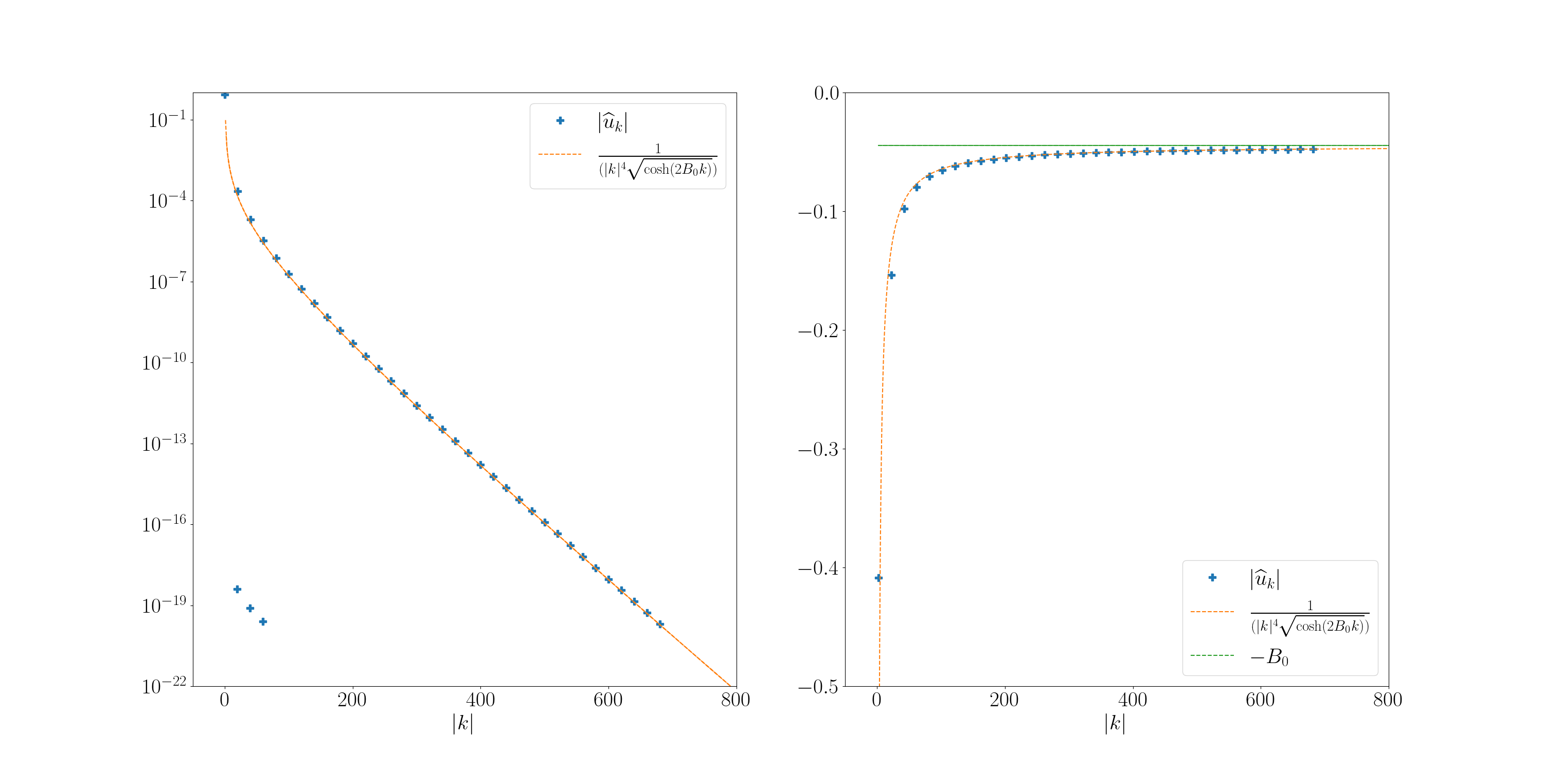
Figure 1. [Linear eigenvalue problem] (Left) Fourier coefficients of (the numerical approximation of) $u_{1}$: they seem to decrease like $1/(\left|k\right|^{\alpha}\sqrt{\cosh{2B_{0}k}})$ with $\alpha=4$, the prefactor $2B_{0}$ in the cosh being confirmed by the plot on the right. (Right) Logarithm of the ratio of two successive nonzero Fourier coefficients.

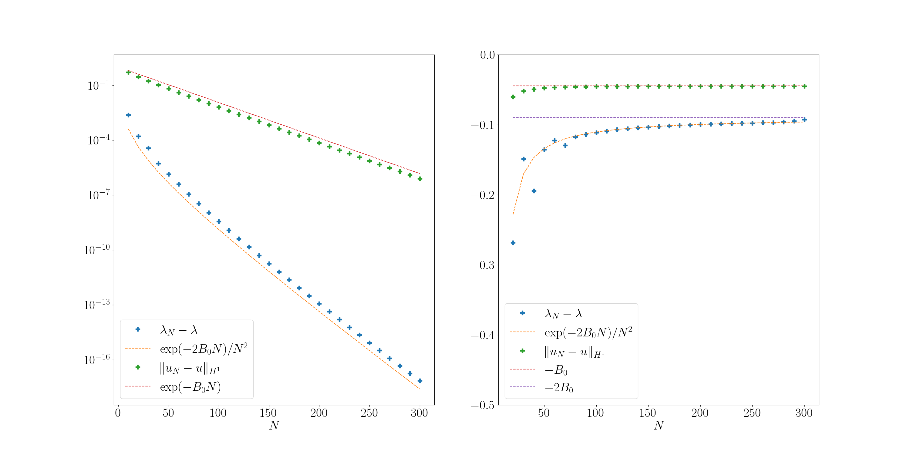
Figure 2. [Linear eigenvalue problem] (Left) Discretization error for the first eigenvalue and the associated eigenvector in the $H^{1}$ norm. Both errors seem to converge with rates given by Theorem 3, the prefactors in the $\cosh$ being confirmed by the plot on the right. (Right) Logarithm of the ratio between discretization errors for various $N$’s.

4. The nonlinear case

In the nonlinear case, the analyticity strip of the solution can be much smaller than the one of the data. First, we report numerical simulations on a nonlinear periodic Gross–Pitaevskii eigenvalue problem with a cubic nonlinearity and a potential admitting an entire continuation, illustrating the fact that the eigenfunction belongs to $\mathcal{H}_{A}$ for some $A>0$, but does not seem to be entire. Next, we study a nonlinear Schrödinger equation with entire potential and source term and cubic nonlinearity. We show that the solution is not entire and we provide an upper bound of the width of the horizontal analyticity strip of the solution.

4.1. Analyticity on a strip

We consider here the nonlinear eigenvalue problem

$$-\Delta u+Vu+|u|^{2}u=\lambda u,\quad\left\|u\right\|_{L^{2}_{\rm per}(\mathbb{R},\mathbb{C})}=1,$$ (12)

where $V\in\mathcal{H}_{B}$ for any $B>0$ is real-valued. Similarly to the linear case, we consider the planewave variational approximation: using again

$$X_{N}\leavevmode\nobreak\ =\leavevmode\nobreak\ \mbox{Span}(e_{k},\leavevmode\nobreak\ \;\leavevmode\nobreak\ |k|\leavevmode\nobreak\ \leqslant\leavevmode\nobreak\ N),$$

we obtain the finite-dimensional problem

$$\begin{cases}\text{seek }(u_{N},\lambda_{N})\in X_{N}\times\mathbb{R}\text{ such that }\left\|u_{N}\right\|_{L^{2}_{\rm per}(\mathbb{R},\mathbb{C})}=1\text{ and }\\ \displaystyle{\forall\ v_{N}\in X_{N},\quad\int_{0}^{2\pi}\overline{\nabla u_{N}}\cdot\nabla v_{N}+\int_{0}^{2\pi}V\overline{u_{N}}v_{N}+\int_{0}^{2\pi}|u_{N}|^{2}\overline{u_{N}}v_{N}=\lambda_{N}\int_{0}^{2\pi}\overline{u_{N}}v_{N}.}\end{cases}$$ (13)

Then, the following theorem holds, which is a simple corollary of known results on the analyticity of elliptic partial differential equations. Note that this result only yields the existence of a finite strip of analyticity in the complex plane. However, even if the data is entire, there is a priori no reason for the solution to be entire too, as shown by the counter-examples that follow.

Theorem 4.

Let $V$ real-valued be in $\mathcal{H}_{B}$ for any $B>0$ and $(u,\lambda)\in H^{2}_{\rm per}(\mathbb{R},\mathbb{R})\times\mathbb{R}$ be the ground-state of (12), uniquely defined under the assumption that $u>0$. Then, there exists $A>0$ such that $u\in\mathcal{H}_{A}$. Moreover, if $(u_{N},\lambda_{N})$ is the variational approximation of $(u,\lambda)$ in $X_{N}\times\mathbb{R}$, then

$$\exists\ C_{A}>0,\quad\left\|u-u_{N}\right\|_{H^{1}_{\rm per}}\leqslant C_{A}\exp(-AN).$$

Proof.

Existence and uniqueness of $u$ is a classical result, proved for instance in [6, Appendix]. In addition, as $V\in H^{s}_{\rm per}(\mathbb{R},\mathbb{R})$ for any $s>0$, we know from [6, Theorem 2] and by an immediate bootstrap argument that $u$ also belongs to $H^{s}_{\rm per}(\mathbb{R},\mathbb{R})$ for any $s>0$. Therefore, $u\in C^{\infty}_{\rm per}(\mathbb{R},\mathbb{R})$.

Knowing that $u\in C^{\infty}_{\rm per}(\mathbb{R},\mathbb{R})$ yields that $u$ is real-analytic on a neighborhood of every point $x_{0}$ of the periodicity cell $[0,2\pi]$, according to well-known results on the analyticity of solutions to nonlinear elliptic equations, which we recall here for the reader’s convenience (see for instance [4, Theorem 1.1], [13, Theorem 1] or [8, 16, 17]).

Theorem 5.

Let $\Omega$ be an open subset of $\mathbb{R}^{n}$, $D$ an open subset of $\mathbb{R}^{n}\times\mathbb{R}\times\mathbb{R}^{n}\times\mathbb{R}^{n\times n}_{\rm sym}$, $F:D\ni(x,v,g,M)\mapsto F(x,v,g,M)\in\mathbb{R}$ a real analytic function, and $u\in C^{\infty}(\Omega)$ a real-valued function such that for all $x\in\Omega$, $(x,u(x),\nabla u(x),\nabla^{2}u(x))\in D$. Assume that $u$ solves $F(x,u(x),\nabla u(x),\nabla^{2}u(x))=0$ and that this equation is elliptic in the sense that

$$\forall(x,\xi)\in\Omega\times\mathbb{R}^{n},\;\xi\neq 0,\quad\xi^{T}\nabla_{M}F(x,u(x),\nabla u(x),\nabla^{2}u(x))\xi\neq 0.$$

Then $u$ is real-analytic in $\Omega$.

By a compactness argument, we therefore have that $u$ is analytic on a strip of size $A>0$ around the real axis, for some $A>0$.

We now consider the variational approximation $(u_{N},\lambda_{N})$ of $(u,\lambda)$ in $X_{N}\times\mathbb{R}$. We know from [6, Theorem 1] that there exists $C>0$ such that

$$\left\|u-u_{N}\right\|_{H^{1}_{\rm per}}\leqslant C\left\|u-\Pi_{N}u\right\|_{H^{1}_{\rm per}}.$$

The result then follows similarly to the proof of Theorem 3. ∎

Remark 2.

In order to establish the convergence rate of the eigenvalues of the ground-state of (12), one can follow the proof of [6, Theorem 2]. Using in particular equations (50) and (53) from this reference, with the negative Sobolev norms replaced by the dual norms of $\mathcal{H}_{A}$, one can obtain that there exists $C_{A}>0$ such that $\left|\lambda-\lambda_{N}\right|\leqslant C_{A}\exp(-2AN)$.

4.2. Counter-examples

We analyze in this section two counter-examples of Theorems 1 and 2 based on the nonlinear Gross–Pitaevskii equation with entire potentials and source terms, for which the solutions are not entire. We also present numerical tests to support our analysis.

4.2.1. A nonlinear Gross–Pitaevskii eigenvalue problem

We study in this section the following nonlinear eigenvalue problem:

$$\begin{cases}-\varepsilon\Delta u_{\varepsilon}+\gamma\cos(x)u_{\varepsilon}+|u_{\varepsilon}|^{2}u_{\varepsilon}=\lambda_{\varepsilon}u_{\varepsilon}\quad\mbox{in }H^{1}_{\rm per}(\mathbb{R},\mathbb{C}),\\ \left\|u_{\varepsilon}\right\|_{L^{2}_{\rm per}}=1,\quad u_{\varepsilon}>0,\end{cases}$$ (14)

with entire data. In view of the results we obtained in the linear case, we could expect the solution $u_{\varepsilon}$ to (14) (which we know to exist) to be entire. However, our numerical experiments suggest on the contrary that $u_{\varepsilon}$ is analytic only on a band of finite size.

The potential $V$ being real-valued, $u_{\varepsilon}$ is actually real-valued too and the singular limit $\varepsilon\to 0$ yields the algebraic equation $\gamma\cos(x)u_{0}(x)+u_{0}(x)^{3}=\lambda_{0}u_{0}(x)$. If we assume that $u_{0}$ does not vanish on the unit cell $[0,2\pi]$, we can divide by $u_{0}(x)$ and then integrate over $[0,2\pi]$: using the normalization condition, we obtain $\lambda_{0}=1/2\pi$. This yields

$$u_{0}(x)=\sqrt{\frac{1}{2\pi}-\gamma\cos(x)},$$ (15)

which is indeed bounded away from zero as soon as $\beta_{0}\coloneqq 1/(2\pi\gamma)>1$, which we take in the following. The analytic continuation of $u_{0}$, still denoted by $u_{0}$, satisfies

$$\gamma\cos(z)u_{0}(z)+u_{0}(z)^{3}=\frac{1}{2\pi}u_{0}(z),$$

with $\sqrt{\cdot}$ in (15) being the continuation of the square root with branch cut $\mathbb{R}_{-}$. The maximal horizontal strip of the complex plane on which $u_{0}$ is analytic is $\mathbb{R}+{\rm i}(-B_{0},B_{0})$, where $B_{0}$ is such that $\cos(\pm{\rm i}B_{0})=\beta_{0}$, that is to say $B_{0}=\log\left(\beta_{0}+\sqrt{\beta_{0}^{2}-1}\right)$. More precisely, the function $z\mapsto u_{0}(z)$ admits two branching points at $z_{\pm}=\pm{\rm i}B_{0}$, for which $u_{0}(z_{\pm})=0$ and

$$\left|\frac{{\rm d}u_{0}}{{\rm d}t}(tz_{\pm})\right|=\left|\frac{\gamma\sin(tz_{\pm})}{2\sqrt{\frac{1}{2\pi}-\gamma\cos(tz_{\pm})}}\right|\to\infty\quad\mbox{when $\mathbb{R}\ni t\to 1_{-}$},$$

see Figure 3.

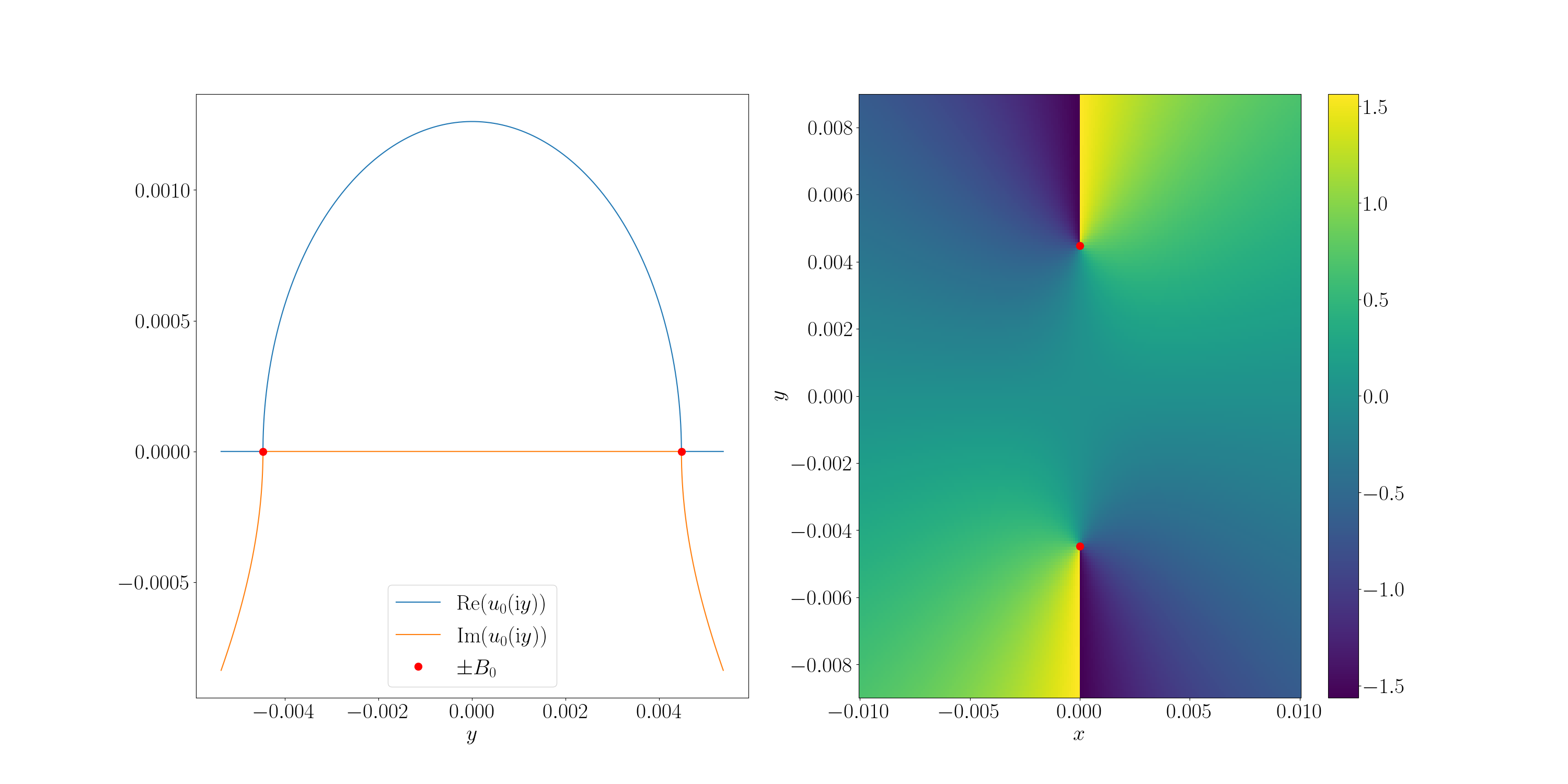
Figure 3. [Nonlinear eigenvalue problem] Analytic continuation of $u_{0}$ for $\beta_{0}=1.00001$, for which $B_{0}\approx 0.0045$. (Left) Imaginary and real parts of $y\mapsto u_{0}({\rm i}y)$. A discontinuity of the derivative appears at the expected positions. (Right) Phase of $z\mapsto u_{0}(z)$ where $z=x+{\rm i}y$. Branching points, in red, appear at the expected positions.

When $\varepsilon>0$, we can approximate numerically the solution of (14) using the planewave approximation presented before, with discretization parameter $E_{\rm cut}=10^{6}$ and solver tolerance $10^{-13}$. The Fourier coefficients of the numerical solution for various $\varepsilon$ are displayed in Figure 4. Although it is not possible to rule out a transition to a different asymptotic regime in the limit of extremely small values of $\varepsilon$ or very large values of $k$ because of finite numerical accuracy, our numerical results are compatible with the decay of the Fourier coefficients of $u_{\varepsilon}$ as $1/(|k|^{3/2}\sqrt{\cosh(2B_{0}k)})$. This leads to the conclusion that the solution $u_{\varepsilon}$ is analytic on a band strip of size close to $B_{0}$, which is in contradiction with the results from the linear case. In the next section, we study a similar nonlinear elliptic equation where we reach similar conclusions and where, in addition, we can provide an upper bound of the width of the horizontal strip on which the solutions are analytic.

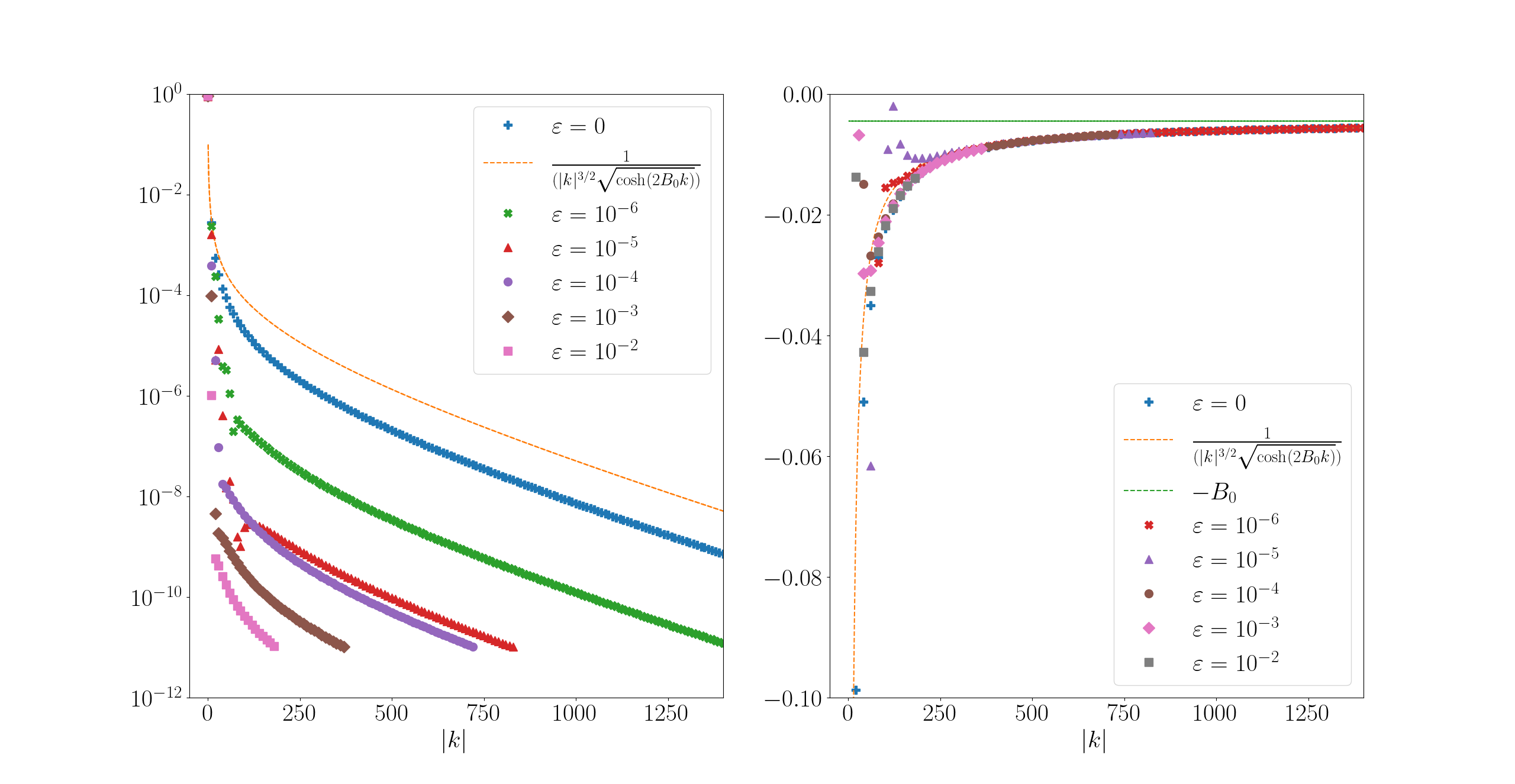
Figure 4. [Nonlinear eigenvalue problem] (Left) Fourier coefficients of (the numerical approximation of) $u_{\varepsilon}$: they seem to decrease like $1/(\left|k\right|^{\alpha}\sqrt{\cosh(2B_{0}k)})$ with $\alpha=3/2$, the prefactor $2B_{0}$ in the $\cosh$ being confirmed by the plot on the right. (Right) Logarithm of the ratio of two successive nonzero Fourier coefficients.

4.2.2. A nonlinear elliptic equation

Still in the perspective of studying nonlinear elliptic problems with analytic data, we now consider the nonlinear periodic elliptic equation with cubic nonlinearity

$$-\varepsilon\Delta u_{\varepsilon}+u_{\varepsilon}+|u_{\varepsilon}|^{2}u_{\varepsilon}=f\quad\mbox{in }H^{1}_{\rm per}(\mathbb{R},\mathbb{C}),$$ (16)

where $\varepsilon>0$, and $f:\mathbb{R}\to\mathbb{R}$ is a real-analytic $2\pi$-periodic function admitting an entire continuation, still denoted by $f$, to the complex plane. We will show that, in this particular case, the same kind of results we showed for the linear case are not true any more and we provide an estimation of the width of the horizontal analyticity strip of the solution, which is finite even though the source term $f$ is entire.

The right-hand-side $f$ being real-valued, $u_{\varepsilon}$ is also real-valued and the singular limit $\varepsilon=0$ gives rise to the algebraic equation $u_{0}(x)+u_{0}(x)^{3}=f(x)$, which has a unique real solution for each $x\in\mathbb{R}$. The latter can be computed by Cardano’s formula: the discriminant of the cubic equation is

$$R(x)=-\left(4+27f^{2}(x)\right)<0,$$

so that

$$u_{0}(x)=\sqrt[3]{\frac{1}{2}\left(f(x)+\sqrt{\frac{-R(x)}{27}}\right)}+\sqrt[3]{\frac{1}{2}\left(f(x)-\sqrt{\frac{-R(x)}{27}}\right)},$$ (17)

the other two roots being complex conjugates with nonzero imaginary parts. The function $u_{0}$ can be analytically continued from the real axis upwards in the complex plane as long as $R(z)$ does not touch zero; it has branching points (with an exploding first derivative) at the points where $R(z)=0$. In the rest of this section, we will use the function $f(x)=\mu\sin(x)$, for a fixed $\mu>0$. The analytic continuation of $u_{0}$ has branching points at $2\pi\mathbb{Z}\pm{\rm i}B_{0}$, with

$$B_{0}={\rm arcsinh}{\sqrt{\frac{4}{27\mu^{2}}}}>0.$$

In particular, although the source term $f$ has an entire continuation, the solution $u_{0}$ given by (17) does not.

When $\varepsilon>0$, we can approximate numerically the solution to (16) with the planewave approximation introduced before, with discretization parameter $E_{\rm cut}=10^{6}$ and solver tolerance $10^{-13}$. The Fourier coefficients of the numerical solution are then displayed in Figure 6 for various $\varepsilon$: the plots suggest that increasing $\varepsilon$ increases the width $B_{\varepsilon}$ of the horizontal analyticity strip of $u_{\varepsilon}(z)$, but does not make it entire.

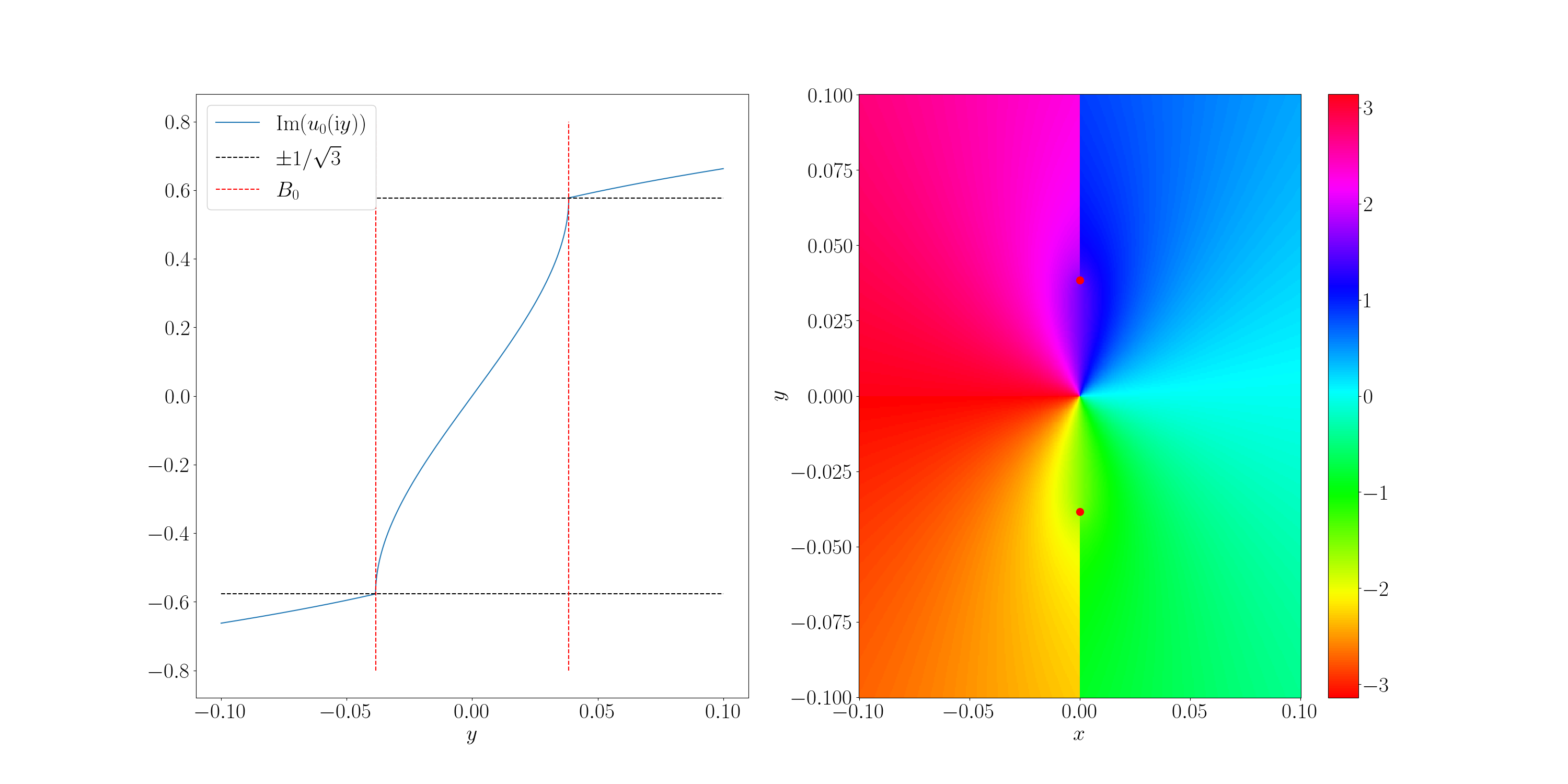
Figure 5. [Nonlinear elliptic equation] Analytic continuation of $u_{0}$ for $\mu=10$, for which $B_{0}\approx 0.0385$. (Left) Imaginary part of $y\mapsto u_{0}({\rm i}y)$. Discontinuities also appear at the expected positions $\pm B_{0}$. (Right) Phase of $z\mapsto u_{0}(z)$ where $z=x+{\rm i}y$. Branching points, in red, appear at the expected positions $\pm{\rm i}B_{0}$.

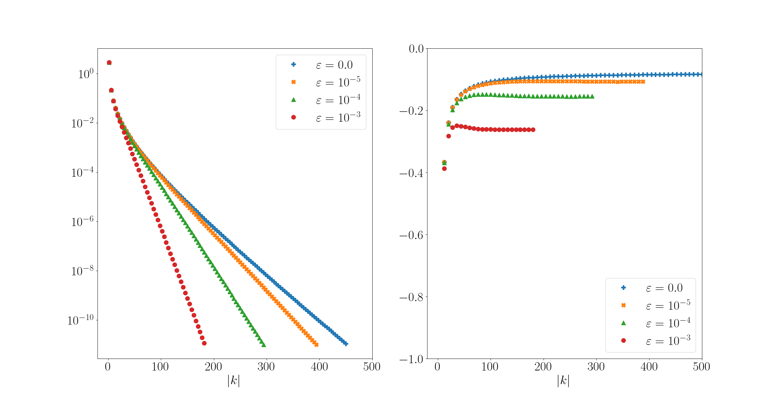
Figure 6. [Nonlinear elliptic equation] (Left) Fourier coefficients of (the numerical approximation of) $u_{\varepsilon}$. (Right) Logarithm of the ratio of two successive nonzero Fourier coefficients.

In this particular case, we are able to obtain an upper bound of the value of $B_{\varepsilon}$ by an ODE technique. Let $\varphi_{\varepsilon}(y)\coloneqq u_{\varepsilon}({\rm i}y)$ be the value of the solution along the imaginary axis. Using the Cauchy–Riemann equations, we see that $\varphi_{\varepsilon}$ satisfies the following second-order ODE:

$$\begin{cases}\varepsilon{\varphi}_{\varepsilon}^{\prime\prime}(y)+\varphi_{\varepsilon}(y)+\varphi_{\varepsilon}^{3}(y)={\rm i}\mu\sinh(y),\\ \varphi_{\varepsilon}(0)=u_{\varepsilon}(0)=0,\quad\varphi^{\prime}_{\varepsilon}(0)={\rm i}u^{\prime}_{\varepsilon}(0),\end{cases}$$

with $u^{\prime}_{\varepsilon}(0)\in\mathbb{R}$. Decomposing $\varphi_{\varepsilon}$ in its real part $\theta_{\varepsilon}$ and imaginary part $\psi_{\varepsilon}$, we see that $\theta_{\varepsilon}$ satisfies the equation

$$\begin{cases}\varepsilon{\theta}^{\prime\prime}_{\varepsilon}+\theta_{\varepsilon}+\theta_{\varepsilon}^{3}-3\theta_{\varepsilon}\psi_{\varepsilon}^{2}=0,\\ \theta_{\varepsilon}(0)=0,\quad\theta^{\prime}_{\varepsilon}(0)=0,\end{cases}$$

and therefore vanishes. As a consequence, $u_{\varepsilon}$ is purely imaginary along the imaginary axis (as could have been anticipated by the symmetries $u_{\varepsilon}(-z)\leavevmode\nobreak\ =\leavevmode\nobreak\ -\leavevmode\nobreak\ u(z)$, $u_{\varepsilon}(\overline{z})=\overline{u_{\varepsilon}(z)}$). We are then left with studying the imaginary part $\psi_{\varepsilon}$, which satisfies the ODE

$$\begin{cases}\varepsilon{\psi}^{\prime\prime}_{\varepsilon}+\psi_{\varepsilon}-\psi_{\varepsilon}^{3}=\mu\sinh,\\ \psi_{\varepsilon}(0)=0,\quad\psi^{\prime}_{\varepsilon}(0)=u^{\prime}_{\varepsilon}(0).\end{cases}$$ (18)

If we can prove that $\psi_{\varepsilon}$ becomes non-analytic at a finite $0<Y_{\varepsilon}<\infty$, this will imply that the width $B_{\varepsilon}$ of the horizontal analyticity strip of $u_{\varepsilon}$ satisfies $B_{\varepsilon}\leqslant Y_{\varepsilon}<\infty$ and is therefore finite even though the data in (16) is entire. To this end, we prove in the Appendix B the following lemma, which gives a sufficient condition for the non-analyticity of $\psi_{\varepsilon}$ in finite time.

Lemma 1.

Let $Y_{\varepsilon}\in\mathbb{R}_{+}\cup\{\infty\}$ be the maximum time of definition of $\psi_{\varepsilon}$. If, for some $\eta>0$ small enough, there exists $y_{\eta}\geqslant B_{0}$ such that $\psi_{\varepsilon}(y_{\eta})=1+\eta>1$ and $\psi_{\varepsilon}^{\prime}(y_{\eta})>0$, then $Y_{\varepsilon}<\infty$ and $\psi_{\varepsilon}(y)\to\infty$ when $y\to Y_{\varepsilon}$.

To prove that the sufficient condition from Lemma 1 is satisfied, we introduce the set

$$X_{\mu}=\left\{(y,\upsilon)\in\mathbb{R}^{2},\ \mu\sinh(y)-\upsilon+\upsilon^{3}\geqslant 0\right\}.$$

This set is such that, if $(y,\psi_{\varepsilon}(y))$ lies strictly inside $X_{\mu}$, then $\psi_{\varepsilon}$ is locally strictly convex. For $y<B_{0}$, $\psi_{\varepsilon}$ might oscillate on both sides of the boundary of $X_{\mu}$ [26]. We investigated numerically the behavior of this function for the set of parameters used in Figure 7 ($\varepsilon=0.1$, $\mu=0.5$), and observed that $0<\psi_{\varepsilon}(B_{0})<\frac{1}{\sqrt{3}}$ and $\psi^{\prime}_{\varepsilon}(B_{0})>0$. This numerical observation can be trusted as the ODE satisfied by $\psi^{\prime}_{\varepsilon}$ on the interval $[0,B_{0}]$ for $\varepsilon=0.1$ and $\mu=0.5$ is not stiff. It is therefore easy to solve it numerically with high accuracy with a posteriori error estimates guaranteeing that $\psi_{\varepsilon}(B_{0})$ is indeed strictly between $0$ and $\frac{1}{\sqrt{3}}$, and $\psi^{\prime}_{\varepsilon}(B_{0})$ is positive. Therefore, $\psi_{\varepsilon}$ is locally strictly convex at $y=B_{0}$. Given the shape of $X_{\mu}$ (see Figure 7 in appendix), $\psi_{\varepsilon}$ lies, for any $B_{0}<y<Y_{\varepsilon}$, above its tangent at $y=B_{0}$, whose slope is $\psi^{\prime}_{\varepsilon}(B_{0})>0$. Strict convexity allows one to conclude that for any $\eta>0$, there exists $y_{\eta}>B_{0}$ such that

$$\begin{cases}\psi_{\varepsilon}(y_{\eta})=1+\eta>1,\\ \psi_{\varepsilon}^{\prime}(y_{\eta})>\psi_{\varepsilon}^{\prime}(B_{0})>0.\end{cases}$$

Any $\eta>0$ is therefore suitable to apply Lemma 1 and conclude that $\psi_{\varepsilon}$ blows up in finite time $Y_{\varepsilon}$. We can deduce from these investigations that $u_{\varepsilon}$ is analytic only on a horizontal strip of finite width of the complex plane although the source term $f$ is an entire function: our results in the linear case are therefore no longer valid in general in the nonlinear case.

Conflict of interest

All the authors declare that they have no conflicts of interest.

Data availability

All the scripts used to generate the plots of Figures 1, 2, 3, 4, 5 and 6 are available online at

https://github.com/gkemlin/analytic_potentials.

Appendix A Extension to the multidimensional case with application to Kohn–Sham models.

The goal of this section is to extend the previous results to the multidimensional case and apply them to the linear version of the Kohn–Sham equations (1). To this end, consider a Bravais lattice $\mathbb{L}=\mathbb{Z}\bm{a}_{1}+\cdots+\mathbb{Z}\bm{a}_{d}$ where $\bm{a}_{1},\dots,\bm{a}_{d}$ are linearly independent vectors of $\mathbb{R}^{d}$ ($d=3$ for KS-DFT). Up to an affine change of variables (which preserves analyticity), we can take without loss of generality $\mathbb{L}=2\pi\mathbb{Z}^{d}$. We denote by $\Omega=[0,2\pi)^{d}$ a unit cell, by $\mathbb{L}^{*}=\mathbb{Z}^{d}$ the reciprocal lattice, by $e_{\bm{G}}(\bm{x})=|\Omega|^{-1/2}{\rm e}^{{\rm i}\bm{G}\cdot\bm{x}}$ the Fourier mode with wavevector $\bm{G}\in\mathbb{L}^{*}$, and by

$$H^{s}_{{\rm per},\mathbb{L}}\coloneqq\left\{u=\sum_{\bm{G}\in\mathbb{L}^{*}}\widehat{u}_{\bm{G}}e_{\bm{G}}\;\middle|\;\sum_{\bm{G}\in\mathbb{L}^{*}}(1+|\bm{G}|^{2})^{s}|\widehat{u}_{\bm{G}}|^{2}<\infty\right\}$$

the $\mathbb{L}$-periodic Sobolev spaces endowed with their usual inner products. All the arguments in Sections 3.1-3.3 can be extended to the multidimensional case by introducing the Hilbert spaces

$$\mathcal{H}_{A,\mathbb{L}}\coloneqq\left\{u\in L^{2}_{{\rm per},\mathbb{L}}\;\middle|\;\sum_{\bm{G}\in\mathbb{L}}{w}_{A,\mathbb{L}}(\bm{G})\left|\widehat{u}_{\bm{G}}\right|^{2}<\infty\right\},\quad(u,v)_{A,\mathbb{L}}\coloneqq\sum_{\bm{G}\in\mathbb{L}^{*}}{w}_{A,\mathbb{L}}(\bm{G})\overline{\widehat{u}_{\bm{G}}}\widehat{v}_{\bm{G}},$$

where $\displaystyle{{w}_{A,\mathbb{L}}(\bm{G})=\sum_{n=1}^{d}w_{A}(G_{n})}$. Each $u\in\mathcal{H}_{A,\mathbb{L}}$ can be extended to an analytic function $u(z_{1},\dots,z_{d})$ of $d$ complex variables defined on a neighborhood on $\mathbb{R}^{d}$, and it holds

$$\sum_{\bm{G}\in\mathbb{L}^{*}}w_{A,\mathbb{L}}(\bm{G})\left|\widehat{u}_{\bm{G}}\right|^{2}=\frac{1}{2}\sum_{j=1}^{d}\int_{\Omega}\left|{u}(\bm{x}+{\rm i}e_{j})\right|^{2}+\left|{u}(\bm{x}-{\rm i}e_{j})\right|^{2}{\rm d}\bm{x}.$$

with $e_{1},\dots,e_{d}$ the canonical basis vectors. The approximation space $X_{N,\mathbb{L}}$ is then defined as

$$X_{N,\mathbb{L}}\coloneqq\mbox{Span}(e_{\bm{G}},\;\bm{G}\in\mathbb{L}^{*},\;|{\bm{G}}|\leqslant N),$$

and the inverse $T_{22,\mathbb{L}}^{-1}$ of the restriction $T_{22,\mathbb{L}}$ of the operator $-\Delta$ on $L^{2}_{{\rm per},\mathbb{L}}$ to the invariant subspace $X_{N,\mathbb{L}}^{\perp}=\mbox{Span}(e_{\bm{G}},\;\bm{G}\in\mathbb{L}^{*},\;|{\bm{G}}|>N)$ satisfies

$$\|T^{-1}_{22,\mathbb{L}}\|_{\mathcal{L}(X_{N,\mathbb{L}}^{\perp})}=\|T^{-1}_{22,\mathbb{L}}\|_{\mathcal{L}(\mathcal{H}_{A,\mathbb{L}}\cap X_{N,\mathbb{L}}^{\perp})}\leqslant N^{-2}.$$

The proofs of Theorem 1, Theorem 2 and Theorem 3 can thus be straightforwardly adapted to the multidimensional case.

Lastly, if $V\in\mathcal{H}_{B,\mathbb{L}}$ for some $B>0$, the Schrödinger operator $H=-\Delta+V$ considered this time as a Schrödinger operator on $L^{2}(\mathbb{R}^{d},\mathbb{C})$ with an $\mathbb{L}$-periodic potential, can be decomposed by the Bloch transform [22, Section XIII.16] and its Bloch fibers are the self-adjoint operators on $L^{2}_{{\rm per},\mathbb{L}}$ with domain $H^{2}_{{\rm per},\mathbb{L}}$ and form domain $H^{1}_{{\rm per},\mathbb{L}}$ defined as $H_{\bm{k}}=(-{\rm i}\nabla+\bm{k})^{2}+V$. The following result is concerned with the Bloch eigenmodes of the $H_{{\bm{k}}}$’s.

Theorem 6.

Let $B>0$ and $V\in\mathcal{H}_{B,\mathbb{L}}$. For each $\bm{k}\in\mathbb{R}^{d}$, the eigenfunctions of the Bloch fibers $H_{\bm{k}}=(-{\rm i}\nabla+\bm{k})^{2}+V$ of the periodic Schrödinger operator $H=-\Delta+V$ are in $\mathcal{H}_{A,\mathbb{L}}$ for any $0<A<B$. Let $\lambda_{1,\bm{k}}\leqslant\lambda_{2,\bm{k}}\leqslant\cdots$ be the eigenvalues of $H_{\bm{k}}$ counted with multiplicities and ranked in non-decreasing order, and $\lambda_{1,\bm{k},N}\leqslant\lambda_{2,\bm{k},N}\leqslant\cdots\leqslant\lambda_{d_{\mathbb{L},N},\bm{k},N}$ the eigenvalues of the variational approximation of $H_{\bm{k}}$ in the $d_{\mathbb{L},N}$-dimensional space

$$X_{\mathbb{L},\bm{k},N}\coloneqq\mbox{\rm Span}(e_{\bm{G}},\;\bm{G}\in\mathbb{L}^{*},\;|\bm{G}+\bm{k}|\leqslant N).$$

Then, for each $0<A<B$ and $i\in\mathbb{N}^{*}$, there exists a constant $C_{i,A}\in\mathbb{R}_{+}$ such that

$$0\leqslant\max_{\bm{k}\in\Omega^{*}}(\lambda_{i,\bm{k},N}-\lambda_{i,\bm{k}})\leqslant C_{i,A}{\rm e}^{-2AN},$$ (19)

where $\Omega^{*}$ is the first Brillouin zone (i.e. the Voronoi cell of the lattice $\mathbb{L}$ of $\mathbb{R}^{d}$ containing the origin).

Proof.

It suffices to replace in the proofs of Theorem 2 and Theorem 3 $X_{N}$ with $X_{\mathbb{L},\bm{k},N}$ and $T_{22}$ with the restriction $T_{22,\mathbb{L},\bm{k}}$ of the operator $(-{\rm i}\nabla+\bm{k})^{2}$ to the invariant space $X_{\mathbb{L},\bm{k},N}^{\perp}$. The latter is invertible and such that $\|T_{22,\mathbb{L},\bm{k}}^{-1}\|_{\mathcal{L}(X_{\mathbb{L},\bm{k},N}^{\perp})}\leqslant N^{-2}$ and $\|T_{22,\mathbb{L},\bm{k}}^{-1}\|_{\mathcal{L}(\mathcal{H}_{A,\mathbb{L}}\cap X_{\mathbb{L},\bm{k},N}^{\perp})}\leqslant N^{-2}$. The result then follows similarly. ∎

Remark 3.

As a conclusion, let us mention that, under appropriate assumptions, we can extend these results to the KS-DFT equations (1) with GTH pseudopotentials in the case where an analytic parametrization of the exchange-correlation functional is used. This is relevant for instance when studying condensed-phase systems, for which the periodic setting is well suited, and where the commonly used approximations of $V_{{\rm xc},\rho}$ are analytic on the positive density values that are of interest in such cases [19]. Then we can rewrite (1) as a system of elliptic PDEs:

$$\begin{cases}\displaystyle\left(-\frac{1}{2}\Delta+V_{\rm nl}+V_{\rm loc}+V_{{\rm H},\rho}+V_{{\rm xc},\rho}\right)\varphi_{i}-\lambda_{i}\varphi_{i}=0,\quad(\varphi_{i},\varphi_{j})_{L^{2}_{{\rm per},\mathbb{L}}}=\delta_{ij},\\ \displaystyle\rho(\bm{x})=\sum_{i=1}^{N_{\rm p}}|\varphi_{i}(\bm{x})|^{2},\\ \displaystyle-\Delta V_{{\rm H},\rho}(\bm{x})=4\pi\left(\rho(\bm{x})-\frac{1}{|\Omega|}\int_{\Omega}\rho\right),\quad\int_{\Omega}V_{{\rm H},\rho}=0,\end{cases}$$

We can then use known results for elliptic systems of PDEs [16, 17] to conclude, in a way similar to what we proved in Theorem 4, that the orbitals $\varphi_{i}$ belong to $\mathcal{H}_{A,\mathbb{L}}$ for some $A>0$. In particular, this leads to the exponential convergence of planewave approximations, justifying the use of GTH pseudopotentials.

Appendix B Proof of Lemma 1

We start by rewriting (18) as a first-order ODE on $\Psi_{\varepsilon}(y)\coloneqq\begin{bmatrix}\psi_{\varepsilon}(y)\\ \psi^{\prime}_{\varepsilon}(y)\end{bmatrix}\in\mathbb{R}^{2}$, starting at $y_{\eta}\geqslant B_{0}$:

$$\Psi^{\prime}_{\varepsilon}(y)=\begin{bmatrix}\Psi_{\varepsilon,2}(y)\\ \varepsilon^{-1}\left(\mu\sinh(y)-\Psi_{\varepsilon,1}(y)+\Psi_{\varepsilon,1}^{3}(y)\right)\end{bmatrix},\qquad\Psi_{\varepsilon}(y_{\eta})\coloneqq\begin{bmatrix}\psi_{\varepsilon}(y_{\eta})\\ \psi^{\prime}_{\varepsilon}(y_{\eta})\end{bmatrix}=\begin{bmatrix}1+\eta\\ \psi^{\prime}_{\varepsilon}(y_{\eta})\end{bmatrix}.$$ (20)

We then use the following simplified version of more general comparison results on systems of differential inequalities [27, 28]. In the sequel, the inequality $a\geqslant b$ for two vectors $a,b\in\mathbb{R}^{d}$ means that $a_{i}\geqslant b_{i}$ for all $1\leqslant i\leqslant d$.

Theorem 7.

(See e.g. [27, p. 112]). Let $d\geqslant 1$ and $G:\mathbb{R}^{d}\to\mathbb{R}^{d}$ be locally Lipschitz and quasimonotone in the sense that for all $X,Z\in\mathbb{R}^{d}$,

$$\left(Z_{i}=X_{i}\mbox{ and }X_{j}\leqslant Y_{j}\mbox{ for $j\neq i$}\right)\quad\Rightarrow\quad\left(G(X)\leqslant G(Z)\right).$$

Let $0\leqslant y_{0}<y_{\rm M}\leqslant\infty$ and $\Phi\in C^{1}([y_{0},y_{\rm M}),\mathbb{R}^{d})$ and $\Psi\in C^{1}([y_{0},y_{\rm M}),\mathbb{R}^{d})$ satisfying respectively the ODE

$$\Phi^{\prime}(y)=G(\Phi(y)),\qquad\Phi(y_{0})\in\mathbb{R}^{d},$$

and the differential inequality

$$\Psi^{\prime}(y)\geqslant G(\Psi(y)),\qquad\Psi(y_{0})=\Phi(y_{0}).$$

Then we have

$$\Psi(y)\geqslant\Phi(y).$$

on $[y_{0},y_{\rm M})$.

To apply this result to (20), we introduce the function $G_{\varepsilon}:\mathbb{R}^{2}\to\mathbb{R}^{2}$ defined by

$$\forall\ X=\begin{bmatrix}X_{1}\\ X_{2}\end{bmatrix}\in\mathbb{R}^{2},\quad G_{\varepsilon}(X)=\begin{bmatrix}X_{2}\\ \varepsilon^{-1}(-X_{1}+X_{1}^{3})\end{bmatrix},$$

and the maximal solution $\Phi_{\varepsilon}$ to

$$\Phi^{\prime}_{\varepsilon}(y)=G_{\varepsilon}(\Phi_{\varepsilon}(y)),\qquad\Phi_{\varepsilon}(y_{\eta})=\begin{bmatrix}1+\eta\\ \psi_{\varepsilon}^{\prime}(y_{\eta})\end{bmatrix}.$$ (21)

As $\sinh(y)\geqslant 0$ for all $y\geqslant 0$, we have the following differential inequality:

$$\Psi^{\prime}_{\varepsilon}(y)\geqslant G_{\varepsilon}(\Psi_{\varepsilon}(y)),\qquad\Psi_{\varepsilon}(y_{\eta})=\Phi_{\varepsilon}(y_{\eta}).$$

Note that, by convexity, $\psi_{\varepsilon}(y)\geqslant\psi_{\varepsilon}(y_{\eta})>1$ for $y\geqslant y_{\eta}$: $G_{\varepsilon}$ is indeed quasimonotone on the domain of interest. We are now ready to compute an upper bound of $Y_{\varepsilon}$ with the use of Theorem 7, which yields

$$\forall\ y\geqslant y_{\eta},\ \Psi_{\varepsilon}(y)\geqslant\Phi_{\varepsilon}(y).$$

This leads us to the study of the ODE

$$\begin{cases}\varepsilon\phi^{\prime\prime}_{\varepsilon}=-\phi_{\varepsilon}+\phi_{\varepsilon}^{3}\\ \phi_{\varepsilon}(y_{\eta})=1+\eta,\ \phi^{\prime}_{\varepsilon}(y_{\eta})=\psi^{\prime}_{\varepsilon}(y_{\eta})>0.\end{cases}$$

We have

$$\frac{\varepsilon}{2}\frac{{\rm d}}{{\rm d}y}\left(\phi^{\prime}_{\varepsilon}\right)^{2}=\frac{{\rm d}}{{\rm d}y}\left(-\frac{1}{2}\phi_{\varepsilon}^{2}+\frac{1}{4}\phi_{\varepsilon}^{4}\right),$$

from which we deduce

$$\frac{\varepsilon}{2}(\phi^{\prime}_{\varepsilon})^{2}=\frac{1}{4}\phi_{\varepsilon}^{4}-\frac{1}{2}\phi_{\varepsilon}^{2}+C(\eta),$$

with

$$\begin{split}C(\eta)&=-\frac{1}{4}(1+\eta)^{4}+\frac{1}{2}(1+\eta)^{2}+\frac{\varepsilon}{2}(\psi^{\prime}_{\varepsilon}(y_{\eta}))^{2}\\ &\geqslant-\frac{1}{4}(1+\eta)^{4}+\frac{1}{2}(1+\eta)^{2}+\frac{\varepsilon}{2}(\psi^{\prime}_{\varepsilon}(y_{0}))^{2},\\ \end{split}$$

where $C(\eta)$ is computed from the initial conditions at $y=y_{\eta}$ and $B_{0}<y_{0}<y_{\eta}$ is such that $\psi_{\varepsilon}(y_{0})=1$. Note that $\eta\mapsto-\frac{1}{4}(1+\eta)^{4}+\frac{1}{2}(1+\eta)^{2}+\frac{\varepsilon}{2}(\psi^{\prime}_{\varepsilon}(y_{0}))^{2}$ is decreasing on $\mathbb{R}_{*}^{+}$ and takes the value $\frac{1}{4}+\frac{\varepsilon}{2}(\psi^{\prime}_{\varepsilon}(y_{0}))^{2}>\frac{1}{4}$ at $\eta=0$. Thus, for $\eta>0$ small enough, $C(\eta)\geqslant\frac{1}{4}$ and we have

$$\begin{split}\frac{\varepsilon}{2}(\phi_{\varepsilon}^{\prime})^{2}&\geqslant\frac{1}{4}\phi_{\varepsilon}^{4}-\frac{1}{2}\phi_{\varepsilon}^{2}+\frac{1}{4}=\frac{1}{4}\left(\phi_{\varepsilon}^{2}-1\right)^{2},\end{split}$$

hence

$$\phi_{\varepsilon}^{\prime}\geqslant\frac{1}{\sqrt{2\varepsilon}}\left(\phi_{\varepsilon}^{2}-1\right)\quad\mbox{on }[y_{\eta},Y_{\varepsilon}).$$

Finally, we consider the ODE

$$\xi^{\prime}_{\varepsilon,\eta}=\frac{1}{\sqrt{2\varepsilon}}(\xi_{\varepsilon,\eta}^{2}-1),\qquad\xi_{\varepsilon,\eta}(y_{\eta})=1+\eta,$$

whose solution is

$$\xi_{\varepsilon,\eta}(y)=\frac{1+\frac{2}{\eta}+\exp\left(\frac{y-y_{\eta}}{\sqrt{\varepsilon/2}}\right)}{1+\frac{2}{\eta}-\exp\left(\frac{y-y_{\eta}}{\sqrt{\varepsilon/2}}\right)},$$

which is defined only up to $Y_{\varepsilon,\eta}\coloneqq\sqrt{\frac{\varepsilon}{2}}\log\left(1+\frac{2}{\eta}\right)+y_{\eta}$ . Applying again Theorem 7, we have that $\phi_{\varepsilon}(y)\geqslant\xi_{\varepsilon,\eta}(y)$ for any $y\geqslant y_{\eta}$ such that both functions are still finite. Putting everything together, we obtain that $\psi_{\varepsilon}$ is only defined up to some $Y_{\varepsilon}$ with $B_{0}<Y_{\varepsilon}\leqslant Y_{\varepsilon,\eta}<\infty$ and that

$$\forall\ y\in[y_{\eta},Y_{\varepsilon}),\quad\psi_{\varepsilon}(y)\geqslant\xi_{\varepsilon,\eta}(y).$$ (22)

These results are illustrated on Figure 7, where we plotted the lower bound $\xi_{\varepsilon,\eta}$ for $\varepsilon=0.1$ and $\eta=0.5$ as well as a numerical approximation of $\psi_{\varepsilon}$.

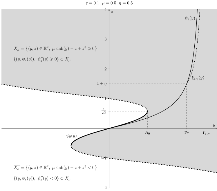
Figure 7. Description of $X_{\mu}$ for $\mu=0.5$, along with the plot of $\psi_{\varepsilon}$ and the lower bound $\xi_{\varepsilon,\eta}$ for $\varepsilon=0.1$, $\eta=0.5$. While $y<B_{0}$, $\psi_{\varepsilon}$ can possibly oscillate around $\psi_{0}$, but as soon as $y\geqslant B_{0}$, $\psi_{\varepsilon}$ is strictly convex and has no other choice than to explode in finite time $Y_{\varepsilon}\leqslant Y_{\varepsilon,\eta}$, where $Y_{\varepsilon,\eta}$ is the explosion time of the lower bound $\xi_{\varepsilon,\eta}$.

References

- [1] I. Babuška and J. Osborn. Eigenvalue problems. In Handbook of Numerical Analysis, volume 2 of Finite Element Methods (Part 1), pages 641–787. Elsevier, 1991.
- [2] C. M. Bender and S. A. Orszag. Advanced Mathematical Methods for Scientists and Engineers. 1: Asymptotic Methods and Perturbation Theory. Springer, New York Heidelberg, 1999.
- [3] S. Bernstein. Sur la nature analytique des solutions des équations aux dérivées partielles du second ordre. Mathematische Annalen, 59(1-2):20–76, 1904.
- [4] S. Blatt. On the analyticity of solutions to non-linear elliptic partial differential systems. arXiv:2009.08762 [math.AP], 2020.
- [5] P. E. Blöchl. Projector augmented-wave method. Physical Review B, 50(24):17953–17979, 1994.
- [6] E. Cancès, R. Chakir, and Y. Maday. Numerical Analysis of Nonlinear Eigenvalue Problems. Journal of Scientific Computing, 45(1):90–117, 2010.
- [7] E. Cancès, R. Chakir, and Y. Maday. Numerical analysis of the planewave discretization of some orbital-free and Kohn-Sham models. ESAIM: Mathematical Modelling and Numerical Analysis, 46(2):341–388, 2012.
- [8] A. Friedman. On the Regularity of the Solutions of Non-Linear Elliptic and Parabolic Systems of Partial Differential Equations. Indiana University Mathematics Journal, 7(1):43–59, 1958.
- [9] P. Giannozzi, S. Baroni, N. Bonini, M. Calandra, R. Car, C. Cavazzoni, D. Ceresoli, G. L. Chiarotti, M. Cococcioni, I. Dabo, A. Dal Corso, S. de Gironcoli, S. Fabris, G. Fratesi, R. Gebauer, U. Gerstmann, C. Gougoussis, A. Kokalj, M. Lazzeri, L. Martin-Samos, N. Marzari, F. Mauri, R. Mazzarello, S. Paolini, A. Pasquarello, L. Paulatto, C. Sbraccia, S. Scandolo, G. Sclauzero, A. P. Seitsonen, A. Smogunov, P. Umari, and R. M. Wentzcovitch. QUANTUM ESPRESSO: A modular and open-source software project for quantum simulations of materials. Journal of Physics. Condensed Matter: An Institute of Physics Journal, 21(39):395502, 2009.
- [10] S. Goedecker, M. Teter, and J. Hutter. Separable dual-space Gaussian pseudopotentials. Physical Review B, 54(3):1703, 1996.
- [11] X. Gonze, B. Amadon, G. Antonius, F. Arnardi, L. Baguet, J.-M. Beuken, J. Bieder, F. Bottin, J. Bouchet, E. Bousquet, N. Brouwer, F. Bruneval, G. Brunin, T. Cavignac, J.-B. Charraud, W. Chen, M. Côté, S. Cottenier, J. Denier, G. Geneste, P. Ghosez, M. Giantomassi, Y. Gillet, O. Gingras, D. R. Hamann, G. Hautier, X. He, N. Helbig, N. Holzwarth, Y. Jia, F. Jollet, W. Lafargue-Dit-Hauret, K. Lejaeghere, M. A. L. Marques, A. Martin, C. Martins, H. P. C. Miranda, F. Naccarato, K. Persson, G. Petretto, V. Planes, Y. Pouillon, S. Prokhorenko, F. Ricci, G.-M. Rignanese, A. H. Romero, M. M. Schmitt, M. Torrent, M. J. van Setten, B. Van Troeye, M. J. Verstraete, G. Zérah, and J. W. Zwanziger. The Abinit project: Impact, environment and recent developments. Computer Physics Communications, 248:107042, 2020.
- [12] C. Hartwigsen, S. Goedecker, and J. Hutter. Relativistic separable dual-space Gaussian pseudopotentials from H to Rn. Physical Review B, 58(7):3641–3662, 1998.
- [13] Y. Hashimoto. A Remark on the Analyticity of the Solutions for Non-Linear Elliptic Partial Differential Equations. Tokyo Journal of Mathematics, 29(2):271–281, 2006.
- [14] M. F. Herbst, A. Levitt, and E. Cancès. DFTK: A Julian approach for simulating electrons in solids. Proceedings of the JuliaCon Conferences, 3(26):69, 2021.
- [15] D. C. Liu and J. Nocedal. On the limited memory BFGS method for large scale optimization. Mathematical Programming, 45(1-3):503–528, Aug. 1989.
- [16] C. B. Morrey. On the Analyticity of the Solutions of Analytic Non-Linear Elliptic Systems of Partial Differential Equations: Part I. Analyticity in the Interior. American Journal of Mathematics, 80(1):198, 1958.
- [17] C. B. Morrey. On the Analyticity of the Solutions of Analytic Non-Linear Elliptic Systems of Partial Differential Equations: Part II. Analyticity at the Boundary. American Journal of Mathematics, 80(1):219, 1958.
- [18] T. Nottoli, I. Giannì, A. Levitt, and F. Lipparini. A robust, open-source implementation of the locally optimal block preconditioned conjugate gradient for large eigenvalue problems in quantum chemistry. Theoretical Chemistry Accounts, 142(8):69, Aug. 2023.
- [19] J. P. Perdew and Y. Wang. Accurate and simple analytic representation of the electron-gas correlation energy. Physical Review B, 45(23):13244–13249, 1992.
- [20] I. G. Petrovskii. Sur l’analyticité des solutions des systèmes d’équations différentielles. Matematiceskij sbornik, 47(1):3–70, 1939.
- [21] L. E. Ratcliff, W. Dawson, G. Fisicaro, D. Caliste, S. Mohr, A. Degomme, B. Videau, V. Cristiglio, M. Stella, M. D’Alessandro, S. Goedecker, T. Nakajima, T. Deutsch, and L. Genovese. Flexibilities of wavelets as a computational basis set for large-scale electronic structure calculations. Journal of Chemical Physics, 152(19):194110, 2020.
- [22] M. Reed and B. Simon. Analysis of Operators. Number 4 in Methods of Modern Mathematical Physics. Academic Press, 1978.
- [23] A. H. Romero, D. C. Allan, B. Amadon, G. Antonius, T. Applencourt, L. Baguet, J. Bieder, F. Bottin, J. Bouchet, E. Bousquet, F. Bruneval, G. Brunin, D. Caliste, M. Côté, J. Denier, C. Dreyer, P. Ghosez, M. Giantomassi, Y. Gillet, O. Gingras, D. R. Hamann, G. Hautier, F. Jollet, G. Jomard, A. Martin, H. P. C. Miranda, F. Naccarato, G. Petretto, N. A. Pike, V. Planes, S. Prokhorenko, T. Rangel, F. Ricci, G.-M. Rignanese, M. Royo, M. Stengel, M. Torrent, M. J. van Setten, B. Van Troeye, M. J. Verstraete, J. Wiktor, J. W. Zwanziger, and X. Gonze. ABINIT: Overview and focus on selected capabilities. Journal of Chemical Physics, 152(12):124102, 2020.
- [24] J. C. Slater. A Simplification of the Hartree-Fock Method. Physical Review, 81(3):385–390, 1951.
- [25] N. Troullier and J. L. Martins. Efficient pseudopotentials for plane-wave calculations. Physical Review B, 43(3):1993–2006, 1991.
- [26] R. Vrabel, P. Tanuska, P. Vazan, P. Schreiber, and V. Liska. Duffing-Type Oscillator with a Bounded from above Potential in the Presence of Saddle-Center Bifurcation and Singular Perturbation: Frequency Control. Abstract and Applied Analysis, 2013:1–7, 2013.
- [27] W. Walter. Ordinary Differential Equations. Number 182 in Graduate Texts in Mathematics ; Readings in Mathematics. Springer, New York, 1998.
- [28] T. Wazewski. Systèmes des équations et des inégualités différentielles ordinaires aux deuxièmes membres monotones et leurs applications. Annales de la Société polonaise de mathématique, 23:112–166, 1950.