Long lived inert Higgs boson in a fast expanding universe and its imprint on the cosmic microwave background

Abstract

Presence of any extra radiation energy density at the time of cosmic microwave background formation can significantly impact the measurement of the effective relativistic neutrino degrees of freedom or ${\rm\Delta N_{eff}}$ which is very precisely measured by the Planck collaboration. Here, we propose a scenario where a long lived inert scalar, which is very weakly coupled to dark sector, decays to a fermion dark matter via freeze-in mechanism plus standard model neutrinos at very low temperature $(T<T_{\rm BBN})$. We explore this model in the fast expanding universe, where it is assumed that the early epoch $(T>T_{\rm BBN})$ of the Universe is dominated by a non-standard species $\Phi$ instead of the standard radiation. In this non-standard cosmological picture, such late time decay of the inert scalar can inject some entropy to the neutrino sector after it decouples from the thermal bath and this will make substantial contribution to ${\rm\Delta{N_{eff}}}$. Besides, in this scenario, the new contribution to $\Delta N_{\rm eff}$ is highly correlated with the dark matter sector. Thus, one can explore such feebly interacting dark matter particles (FIMP) by the precise measurement of $\Delta N_{\rm eff}$ using the current (Planck2018) and forthcoming (CMB-S4 & SPT3G) experiments.

I Introduction

The discovery of the 125 GeV Higgs boson by both ATLAS and CMS collaborations at the LHC completes the basic building blocks of standard model (SM) particle physics, albeit some theoretical and experimental shortcomings. The SM with its present setup is unable to explain the observed non-zero neutrino masses and mixingsT2K:2011ypd ; DoubleChooz:2011ymz ; DayaBay:2012fng ; RENO:2012mkc ; MINOS:2013xrl ; ParticleDataGroup:2020ssz and the existence of dark matter as indicated by various astrophysical and cosmological measurements Zwicky:1933gu ; Rubin:1970zza ; Clowe:2006eq ; Planck:2018vyg . The resolution of these two fundamental puzzles of particle and astroparticle physics beg for an extension of the SM and a plethora of beyond the standard model (BSM) scenarios have been proposed to address these two issues. The neutrino masses and their mixing angles can be easily accommodated at tree level in the three Seesaw mechanisms Minkowski:1977sc ; Mohapatra:1979ia ; Schechter:1980gr ; Gell-Mann:1979vob ; Mohapatra:1980yp ; Lazarides:1980nt ; Wetterich:1981bx ; Schechter:1981cv ; Brahmachari:1997cq ; Foot:1988aq . Note that besides the tree-level seesaw mechanisms, small neutrino masses can also be generated radiatively at one loop level Ma:1998dn ; Ma:2006km .

For a very long time, weakly interacting massive neutral particles (WIMP) Kolb:1990vq ; Feng:2010gw ; Roszkowski:2017nbc ; Schumann:2019eaa ; Lin:2019uvt ; Arcadi:2017kky have been considered as the most coveted candidate for dark matter particle with mass roughly between tens of GeV to a few TeV, and sufficiently large (of the order of electroweak strength) interaction with SM particles. WIMPs provide the observed relic abundance $(\Omega h^{2}\sim 0.1198)$ via the well-known thermal freeze-out mechanism. Non observation of any experimental signal PandaX-II:2016vec ; XENON:2017vdw ; LUX:2016ggv ; PICO:2019vsc ; AMS:2013fma ; Buckley:2013bha ; Gaskins:2016cha ; Fermi-LAT:2016uux ; MAGIC:2016xys ; Bringmann:2012ez ; Cirelli:2015gux ; Kahlhoefer:2017dnp ; Boveia:2018yeb of the DM lead to severe constraints on the WIMP paradigm.

To circumvent these constraints on the WIMP scenario, an alternative framework called freeze-in mechanism has been proposed. In this scenario the dark matter is a feebly interacting massive particle (FIMP) having highly suppressed interaction strength $\lesssim{\cal O}(10^{-12})$ with the SM sector. In the simplest scenario, it is assumed that the initial number density of DM is either zero or negligibly small, and the observed relic abundance is produced non-thermally either from annihilation or decay of SM particles in the early universe. The FIMP freezes in once the temperature drops below the dark matter mass and yields a fixed DM relic abundance that is observed at the present day Hall:2009bx ; Konig:2016dzg ; Biswas:2016bfo ; Biswas:2016iyh ; Bernal:2017kxu ; Borah:2018gjk . FIMP having such a small coupling with the visible sector can trivially accommodate various null results of DM in different direct detection experiments such as PandaPandaX-II:2016vec , XENONXENON:2017vdw , LUXLUX:2016ggv . However, FIMPs imprints can be traced via cosmological observations such as big bang nucleosynthesis (BBN), cosmic microwave background (CMB) or free streaming length Heeck:2017xbu ; Bae:2017dpt ; Boulebnane:2017fxw ; Ballesteros:2020adh ; DEramo:2020gpr ; Decant:2021mhj ; Li:2021okx ; Ganguly:2022ujt .

It would be very interesting to look for a minimal BSM paradigm where both the aforementioned sectors (non-zero neutrino mass and FIMP dark matter) are connected. In some particular scenario, such new interactions of neutrinos can have non-trivial implications in cosmological observations and the precision era of cosmological measurements such as BBN or CMB provide us distinctive possibility for the indirect probe of those hidden particles.

We know that one of the very important and precisely measured observable of the early Universe is the number of effective relativistic neutrino degrees of freedom or ${\rm N_{eff}}$ which can be changed in the presence of non-standard interactions of neutrinos. It is usually parameterised as, ${\rm N_{eff}}\equiv{\left(\rho_{\rm rad}-\rho_{\gamma}\right)}/{\rho_{\nu_{L}}}$, where $\rho_{\rm rad}$, $\rho_{\gamma}$ and $\rho_{\nu_{L}}$ are the total radiation energy density, energy density of photon and the energy density of single active neutrino species respectively. According to the recent data Planck 2018 Planck:2018vyg , at the time of CMB formation ${\rm N_{eff}^{CMB}=2.99^{+0.34}_{-0.33}}$ with 95$\%$ confidence level whereas the SM predicts it to be ${\rm N_{eff}^{SM}=3.045}$ Mangano:2005cc ; Grohs:2015tfy ; deSalas:2016ztq . The departure from 3, the number of neutrinos in the SM, is the consequence of various non-trivial effects like non-instantaneous neutrino decoupling, finite temperature QED corrections to the electromagnetic plasma and flavour oscillations of neutrinos. So, there are still some room to accommodate the contribution from the beyond SM physics. However, future generation CMB experiments like SPT-3GSPT-3G:2019sok , CMB-IVCMB-S4:2016ple are expected to attain a precision of $\rm{\Delta N_{eff}}\approx 0.06$ at 95% confidence level. Thus any new contribution to the radiation energy density can be probed very precisely which can constrain various BSM scenarios that produce light degrees of freedom and are in thermal equilibrium with the SM at early epoch of the evolution of our Universe.

On the other hand, different cosmological events such as decoupling of any relic species from the thermal bath or the non-thermal production of some species are sensitive to evolution history of the Universe. In the standard cosmological picture, it is assumed that after the end of the inflation, the energy density of the Universe is mostly radiation dominated. However, we only have precise information about the thermal history of the Universe at the time of BBN ($T_{\rm BBN}\sim{\rm MeV}$) and afterwards when the Universe was radiation dominated Kawasaki:2000en ; Ichikawa:2005vw . This allows us to consider the possibility that some non-standard species dominated significantly to the total energy budget of the Universe at early times $(T>T_{\rm BBN})$. In that scenario, if the total energy density is dominated by some non-standard species, the Hubble parameter $(H)$ at any given temperature is always larger than the corresponding value of $H$ for the standard cosmology at the same temperature. Such a scenario with larger Hubble parameter is known as the fast expanding universe where at earlier time (higher temperature) the universe was matter dominated and eventually at some lower temperature before BBN radiation density $(\rho_{\rm rad})$ takes over the energy density of the non-standard species ($\rho_{NS}$). One such possibility was discussed in DEramo:2017gpl where $\rho_{NS}$ depends on the scale factor as $\sim a^{-(4+n)}$, where $n>0$. Following the notation of DEramo:2017gpl , this era of the universe is identified by temperature $T_{r}$, where $\rho_{NS}(T_{r})=\rho_{\rm rad}(T_{r})$. Thus, the non-standard cosmological era correspond to the temperature regime where $T>T_{r}$. In the limit, $n=0$ corresponds to the standard radiation dominated cosmological picture. This may be realized by introducing a BSM scalar field $\Phi$ with equation of state(EOS) $p_{\Phi}=\omega\rho_{\Phi}$, where $p_{\Phi},\,\rho_{\Phi}$ denote the pressure and energy density of $\Phi$ respectively and $\omega\in{[-1,1]}$. The energy density prior to BBN red-shifts as follows :

$$\rho_{\Phi}\propto a^{-(4+n)},$$ (1)

where, $n=3\omega-1$. For $\omega>\frac{1}{3}$ this the energy density will fall faster than the radiation. This scenario have been studied in different context in the literature PhysRevD.55.1875 ; PhysRevD.28.1243 ; article ; PhysRevD.37.3406 ; Copeland:1997et ; Bernal:2018kcw . We assume this $\Phi$ has negligible coupling with SM sector only so that the only effect it will have is in the expansion rate of the universe. As the new species red-shifts faster than the radiation. it’s energy density will eventually become subdominant even without the presence of any decay. Several works reported the implications of non-standard cosmological scenarios in context of WIMP relic density calculation DEramo:2017gpl ; Poulin:2019omz ; Redmond:2017tja ; Hardy:2018bph ; Barman:2021ifu ; DEramo:2017ecx ; Bernal:2018kcw . It is observed that if the thermal DM production occurs before $T_{\rm{BBN}}$ when the expansion rate of Universe was larger than radiation dominated(RD) universe, freeze out happens at earlier time thus producing higher relic abundance Poulin:2019omz ; Redmond:2017tja ; Hardy:2018bph . Thus one requires larger coupling of the DM with thermal bath particles to produce higher DM annihilation cross-section at late universe so that it produces the relic density that matches with the observed one. Similar studies in the case of non-thermal production of DM have also been investigated DEramo:2017ecx ; Co:2015pka ; Bernal:2018kcw . Various phenomenological implications of the non standard cosmology have been extensively studied by several groups Berlin:2016vnh ; Tenkanen:2016jic ; Dror:2016rxc ; Berlin:2016gtr .

Motivated by this, we embark on a scenario where the SM particle content is augmented by an inert $SU(2)$ scalar doublet ($\eta$) and three SM gauge singlet fermions $(N_{1},N_{2},N_{3})$ where all of them are odd under a Unbroken $\mathcal{Z}_{2}$ symmetry Ma:2006km ; Borah:2018rca ; Kitabayashi:2021hox ; DeRomeri:2021yjo ; Escribano:2021ymx ; Avila:2021mwg ; Alvarez:2021otp ; Escribano:2021wud ; Hundi:2022iva . The striking feature of this model is the way it connects the origin of neutrino mass and DM. Neutrino mass can arise through one loop radiative seesaw, whereas both $\eta^{0}$, the real component of the scalar doublet, and ${N}$ can be the DM candidate depending on their mass hierarchy. For scalar DM $(\eta^{0})$, different studiesDeshpande:1977rw ; Barbieri:2006dq ; LopezHonorez:2006gr ; Arhrib:2013ela have shown that the correct relic density can be produced only in the high mass region ($M_{\eta^{0}}\gtrsim 525$ GeV). However, this scenario can change if we introduce another real gauge singlet scalar $S$, which is also odd under $\mathcal{Z}_{2}$ symmetry and mixes with $\eta^{0}$. The immediate consequence of such non-trivial mixing between the singlet $(S)$ and $\eta^{0}$ is a newly formed scalar DM $(\eta_{1})$ state as a linear superposition of $\eta^{0}$ and $S$ with suppressed gauge interaction compared to the doublet scalar. As a result of this suppressed gauge coupling, the scalar DM can now have mass as low as $200$ GeV consistent with the observed relic density Beniwal:2020hjc ; Farzan:2009ji ; Ahriche:2016cio .However, both in presence or absence of the singlet scalar, lightest of the singlet fermions $N_{i}$ can be a plausible thermal DM candidate due to their Yukawa interaction with new scalar doublet and the SM leptons. In all such cases, the model faces stringent constraints from different direct detection experiments. As discussed above, motivated by the null results of these experiments, here we study another version of scotogenic model where the DM is produced via non-thermal mechanism. In this analysis, instead of a scalar DM, the lightest singlet ${\mathcal{Z}}_{2}$ odd fermion $N_{1}$ plays the role of the DM, whereas the lightest neutral scalars $(\eta_{1})$, which is the admixture of the real part of the doublet $(\eta^{0})$ and the singlet $(S)$, is very long lived and decays to DM plus one neutrino at very late time (after neutrino decoupling). If the decay happens at sufficiently low temperature, after the decoupling of active neutrinos from the thermal bath, it can significantly affect the total radiation energy density of the universe and contribute to the ${\rm N_{eff}}$. While, calculating the amount of ${\rm\Delta{N_{eff}}}$, we realised that in standard cosmological scenario the remnant abundance of $\eta_{1}$ is not sufficient to produce detectable ${\rm\Delta{N_{eff}}}$ in the present experimental sensitivity. We show that the scenario can be significantly changed if our universe had gone through some non-standard expansion history.

This paper is organized as follows. The section II is devoted for the brief discussion of the basic setup of the model and important interactions. The discussion on dark matter and ${\rm\Delta N_{eff}}$ is presented in the section section III, while the section IV contains our main numerical results. Finally, we conclude in section V.

II Basic set up

The particle spectrum of this model contains a $SU(2)_{L}$ inert doublet scalar ($\eta$), a real singlet scalar ($S$) and three right-handed neutrinos ${N_{i}},(i=1,2,3)$ in addition to the SM particles. We impose an additional $\mathcal{Z}_{2}$ symmetry under which all the SM particles are even whereas the new fields are odd. In this prescription the lightest of these $\mathcal{Z}_{2}$ odd particles will be absolutely stable and be viable DM candidate. With these particles in hand, one can write down the following interaction Lagrangian:

$$\mathcal{L}_{\rm fermion}=y_{i\alpha}\overline{\ell^{i}_{L}}\tilde{\eta}N_{\alpha}+\frac{1}{2}M_{\alpha\beta}\overline{N_{\alpha}^{c}}N_{\beta}+h.c.,$$ (2)

where $\ell^{i}_{L}$ is the SM left handed $SU(2)_{\rm L}$ lepton doublet, $y_{i\alpha}$ is the lepton Yukawa coupling of flavours $i=e,\mu,\tau$, $M_{\alpha\beta}$ is the symmetric Majorana mass matrix and $\tilde{\eta}=i\sigma_{2}\eta^{*}$. The Yukawa interaction, in particular $y_{i1}$ term in equation (2) plays the most important role in the dark matter phenomenology discussed later in this paper. The scalar potential of the model $V(\phi,\eta,S)$, followed by its minimization condition and relevant mass and coupling parameters are shown in Appendix A.

After the electroweak symmetry breaking, two neutral physical eigen states $\eta_{1}$ and $\eta_{2}$ can be expressed as the linear combination of the weak basis $\eta^{0}$ and $S$ as:

$$\eta_{1} = \cos\theta\,\eta_{0}-\sin\theta\,S$$ (3)

$$\eta_{2} = \sin\theta\,\eta_{0}+\cos\theta\,S$$ (4)

where $\theta$ is the neutral CP-even scalar mixing angle. It is obvious that for $\theta=0$, $\eta_{1}(\eta_{2})$ doublet(singlet) dominated and vice-versa for $\theta=\pi/2$. The following parameters describe the scalar sector of this model (see Appendix A for details):

$$M_{\eta_{1}},\ M_{\eta_{2}},\ M_{A^{0}},\ M_{\eta^{+}},\ \lambda_{\eta},\lambda_{S},\ \lambda_{\phi S},\ \lambda_{\eta S},\ \lambda_{3},\ \sin\theta$$ (5)

In addition to these we also have three right handed heavy neutrino masses, $M_{N_{1,2,3}}$. We use the following mass ordering and importance of this particular mass pattern in the context of our phenomenology will be discussed shortly.

$${M_{N_{3}},\,M_{N_{2}},M_{\eta_{2}}>M_{\eta_{1}}>M_{N_{1}}}.$$ (6)

This mass pattern implies that the lightest $\mathcal{Z}_{2}$ odd fermion $N_{1}$ is a suitable candidate for the DM having the Yukawa coupling $y_{i1}$ that features in the production of $N_{1}$ from the decay of $\eta_{1}$.

	$M_{\eta^{\pm}}$ (GeV)	$M_{A^{0}}$ (GeV)	$M_{\eta_{2}}$ (GeV)
BP-1	180	250	400
BP-2	150	200	400
BP-3	180	220	500

Table 1: Values of heavy scalar masses for 3 benchmark points.

To reveal the implications of heavier scalars in our analysis we consider three distinct values of $M_{\eta^{\pm}},M_{A^{0}}$ and $M_{\eta_{2}}$ as represented by three benchmark points BP-1, BP-2 and BP-3 in Table 1.

There is an interesting manifestation of relative mass-splittings among $M_{\eta_{1}}$, $M_{\eta_{2}},M_{A^{0}}$ on the dark matter phenomenology as well as on constraining the model parameter space from the electroweak precision data. As far as heavier neutrino masses $M_{N_{2,3}}$ are concerned, we set them at ${\cal O}(1)$ TeV throughout this analysis so that neutrino masses can be generated radiatively in the right ball park with ${\cal O}(1)$ Yukawa couplings.

Now, a short discussion on the production mechanism of aforesaid heavy particles and how they remain in thermal equilibrium at early universe is called for. Both $\eta_{1}$ and $\eta_{2}$ can be produced in thermal bath of the early universe through their interactions with the SM gauge bosons and Higgs boson. Heavy neutrinos ${N_{i}}$ being gauge singlet can interact with thermal plasma only through $\eta$ and their presence in the thermal bath solely depend on the Yukawa interactions as shown in equation (2). The DM $N_{1}$ is produced non-thermally from the decay of both $\eta_{1}$ and $\eta_{2}$ and the respective decay rates depend on the Yukawa coupling $y_{i1}$ and the corresponding scalar mixing angles $\cos\theta$ and $\sin\theta$. For our choice of benchmark points (see Table 1) $\eta_{2}$ mostly decays to $W^{\pm}\eta^{\mp}$ or $ZA^{0}$ pairs through gauge interactions, leaving negligible contribution towards $N_{1}$ production via Yukawa coupling. Hence, for all practical purposes, $\Gamma(\eta_{2}\to\nu+N_{1})\simeq 0$.

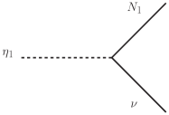
Figure 1: Feynman diagram corresponding to the decay of $\eta_{1}$.

Thus for our choice of $\eta_{1}$ and $N_{1}$ masses, $N_{1}$ will be produced in association with active neutrino from the decay of $\eta_{1}$ (see Fig.1) with $100\%$ branching ratio and the corresponding decay width for one neutrino generation can be written as

$$\Gamma_{\eta_{1}\rightarrow\overline{\nu}N_{1}}=\dfrac{y_{N_{1}}^{2}\cos^{2}{\theta}\,M_{\eta_{1}}}{16\,\pi}\left(1-\dfrac{M_{N_{1}}^{2}}{M_{\eta_{1}}^{2}}\right)^{2},$$ (7)

where, we denote the Yukawa coupling $y_{i1}$ as $y_{N_{1}}$ and will use this notation in rest of the paper. From the functional dependence of $\eta_{1}$ decay width (equation (7)) on $y_{N_{1}}$ it is clear that for the late lime production of $N_{1}$ from the decay of $\eta_{1}$ via freeze-in mechanism, the Yukawa coupling $(y_{N_{1}})$ has to be extremely weak unlike for other two heavy neutrinos $(N_{2}~{}\&~{}N_{3})$ that have $\mathcal{O}(1)$ Yukawa interactions with $\eta$.

In the presence of such large Yukawa couplings, both $N_{2}$ and $N_{3}$ will be produced in thermal equilibrium in the early epoch of the universe and will decay to other lighter $\mathcal{Z}_{2}$ odd particles ($\eta_{1}$, $\eta_{2}$, $\eta^{\pm}$, and $A^{0}$) after their decoupling from the thermal plasma. Hence, these decays would have no impact in the relic abundance of $N_{1}$. So far, we were silent about the production of neutrino in association with $N_{1}$ from decay of long-lived $\eta_{1}$ and its impact on the dynamics of cosmology. The Yukawa coupling $(y_{N_{1}})$ is such that the decay $\eta_{1}\to N_{1}+\nu$ mostly happens after neutrinos decouple from the thermal bath and the decay must also be completed before CMB formation $(T\approx 1~{}{\rm eV})$ so that produced neutrinos in this mechanism have very intriguing implications in the observation of the CMB radiation. To fulfill this condition of $\eta_{1}$ decay, $y_{N_{1}}$ can not take any arbitrary value, rather it should be in the range $(\sim 10^{-15}-10^{-12})$ as considered in our analysis. As a result, this decay will inject entropy to the neutrino sector only and will increase the total radiation energy density of the universe at that epoch. However, any significant increment of total radiation energy density during CMB formation will directly impact ${\rm\Delta N_{eff}}$, as discussed earlier and can be observed in different experiments. The same decay will also set the observed relic density of DM in today’s universe. Hence, the DM mass will decide the amount of energy get transferred to the neutrino sector and can directly be related to $\rm{\Delta N_{eff}}$. The most important parameters of our discussion are $M_{\eta_{1}},\,\lambda_{3},\ \lambda_{\phi S},\ \sin{\theta},\ M_{N_{1}}\,\text{and}\,y_{N_{1}}$. Among these parameters, ${M_{\eta_{1}}}$, $\lambda_{3}$ and $\lambda_{\phi S}$ decide the annihilation cross-sections of $\eta_{1}$, $\sin{\theta}$ decides mixing of the CP even real scalars $\eta^{0}$ and $S$. At the completion of $\eta_{1}$ decay, the final abundance of physical state $\eta_{1}$ gets distributed into DM abundance and active neutrino energy density depending on $M_{N_{1}}$ and $y_{N_{1}}$, thus providing a connection between the DM mass (${M_{N_{1}}}$) and ${\rm\Delta N_{eff}}$, and we will explore this in our current endeavour. As we prefer an enhanced co-moving number density of $\eta_{1}$ in the mass regime $M_{\eta_{1}}\raise 1.29167pt\hbox{$\;>$\kern-7.5pt\raise-4.73611pt\hbox{$\sim\;$}}{60}$ GeV, various co-annihilation processes between dark sector particles must be suppressed in order to avoid any additional enhancement of effective cross-section of $\eta_{1}$ as this would lead to lower abundance of comoving number density of $\eta_{1}$. The lower yield of $\eta_{1}$ in turn produce lower neutrino number density and this may not be sufficient enough to induce observable effect on $\Delta N_{\rm eff}$. Hence, we suppress the above co-annihilation processes by increasing mass splittings between $M_{\eta_{1}}$ and other relevant heavy scalar particles of dark sector. This justifies our choice of associated heavy scalar masses for three benchmarks (BP-1, BP-2 & BP-3) as shown in Table 1.

III Freeze in DM and ${\rm\mathbf{\Delta N_{eff}}}$ at CMB

Following our detailed discussions in previous sections, hereby we address the issue of dark matter $(N_{1})$ abundance created by the late time $(\tau_{\eta_{1}}>t_{\rm BBN})$ decay of $\eta_{1}\to N_{1}+\nu$. Since $N_{1}$ is the dark matter particle, it must satisfy the observed relic abundance at present time and to estimate it one has to solve the following two coupled Boltzmann equations that showcase the evolution of comoving number densities $Y_{\eta_{1}}$ and $Y_{N_{1}}$ corresponding to $\eta_{1}$ and $N_{1}$ respectively with the temperature of the universe:

$$\dfrac{dY_{\eta_{1}}}{dx} = -\dfrac{s}{H(x)x}\left(1-\frac{1}{3}\frac{d\ln g_{s}(x)}{d\ln x}\right)\left<\sigma v\right>_{\rm eff}(Y_{\eta_{1}}^{2}-(Y_{\eta_{1}}^{eq})^{2})$$ (8)

$$-\dfrac{\left<\Gamma_{\eta_{1}\rightarrow N_{1}\nu}\right>}{H(x)x}\left(1-\frac{1}{3}\frac{d\ln g_{s}(x)}{d\ln x}\right)Y_{\eta_{1}},$$

$$\dfrac{dY_{\rm N_{1}}}{dx} = \dfrac{\left<\Gamma_{\eta_{1}\rightarrow N_{1}\nu}\right>}{H(x)x}\left(1-\frac{1}{3}\frac{d\ln g_{s}(x)}{d\ln x}\right)Y_{\eta_{1}}.$$ (9)

where $x=M_{sc}/T$ is a dimensionless variable with $M_{sc}$ is some arbitrary mass scale which doesn’t affect the analysis and we consider it to be 100 GeV. Moreover, ${Y_{\eta_{1}}^{eq}}$ is the equilibrium co-moving number density of $\eta_{1}$, $g_{s}(x)$ and $H(x)$ represent the effective relativistic degrees of freedom related to the entropy density and the expansion rate of the universe respectively. The thermal average of effective annihilation cross-section of $\eta_{1}$ to the bath particles is denoted by $\left<\sigma v\right>_{\rm{eff}}$. The entropy density $s$ and $Y_{i}$’s are related as $Y_{i}=\frac{n_{i}}{s}$ where $n_{i}$’s are the respective number densities. Finally $\left<\Gamma_{\eta_{1}\rightarrow N_{1}\nu}\right>$ denote the thermal average of the decay width given in equation (7). While doing our numerical calculation, we take into account all three active neutrinos in $\left<\Gamma_{\eta_{1}\to N_{1}\nu}\right>$.

The evolution equation of the co-moving number density of $\eta_{1}$ is represented by equation (8). The first term on the right hand side of this equation corresponds to the self annihilation of $\eta_{1}$ into the SM sector and vice versa, which keep $\eta_{1}$ in thermal equilibrium. However, in the presence of a tiny Yukawa coupling, $\eta_{1}$ slowly decays into $N_{1}+\nu$, thus diluting its number density. This feature is reflected in the second term of equation (8). Once the DM $(N_{1})$ is produced in the above decay channel, its thermal evolution is governed by equation (9). Note that in the absence of the Yukawa interaction, $\eta_{1}$ becomes stable and plays the role of the DM, having no effect on $\Delta N_{\rm eff}$, thus not considered in this analysis.

We will now discuss the phenomenological consequence of late-time decay of $\eta_{1}$ into DM and neutrinos which is the motivation of this work. The sufficient production of active neutrinos after it decouples from the thermal bath ($T\raise 1.29167pt\hbox{$\;<$\kern-7.5pt\raise-4.73611pt\hbox{$\sim\;$}}2$ MeV) can hugely affect the total radiation energy density of the universe at that time and will finally increase ${\rm\Delta N_{eff}}$. The effective number of relativistic neutrinos at the time of CMB can be written as:

$$N_{\rm eff}^{\rm CMB}=\frac{8}{7}\left(\frac{11}{4}\right)^{4/3}\frac{\rho_{\nu}}{\rho_{\gamma}}\Bigg{|}_{\rm T=T_{CMB}}.$$ (10)

where $\rm{\rho_{\nu}}$ and $\rm{\rho_{\gamma}}$ are the energy densities of neutrino and photon respectively. The production of $\nu$s from some external source will increase its energy density and we parameterize the deviation from the SM value in the following way:

$$\frac{N_{\rm eff}^{\prime}}{N_{\rm eff}^{\rm SM}}=\frac{\rho_{\nu}^{\prime}}{\rho_{\nu}^{\rm SM}}\Bigg{|}_{\rm T=T_{CMB}},$$ (11)

where $\rm{\rho_{\nu}^{\prime}}$ is the total energy density of neutrinos, i.e. the sum of the SM contribution (${\rho_{\nu}^{\rm SM}}$) and the non-thermal contribution $(\rho_{\nu}^{extra})$ coming from the decay of $\eta_{1}$. Hence, ${\rm\Delta N_{eff}}$ can be expressed as follows,

$$\Delta N_{\rm eff}=\left(\frac{\rho^{\prime}_{\nu}}{\rho^{\rm SM}_{\nu}}-1\right)\,N_{\rm eff}^{\rm SM}\Bigg{|}_{\rm T=T_{CMB}}$$ (12)

To know the temperature evolution of the total neutrino energy density ${\rm\rho_{\nu}^{\prime}}$ after the decay of $\eta_{1}$, we need to solve the following Boltzmann equation:

$$\frac{d\rho^{\prime}_{\nu}}{dx} = -\dfrac{4\,\beta(T)\,\rho^{\prime}_{\nu}}{x}+\frac{1}{xH(x)}\left<E\Gamma\right>_{\eta_{1}\rightarrow N_{1}\nu}Y_{\eta_{1}}s,$$ (13)

where $\beta(T)$ shows the variation of $g_{s}(T)$ with T and is defined as:

$$\beta(T)=1+\frac{1}{3}\frac{T}{g_{s}(T)}\frac{d\,g_{s}(T)}{dT},$$ (14)

and $<E\Gamma>_{\eta_{1}\rightarrow N_{1}\nu}$, term associated with the thermal average of energy density transferred to neutrino sector from $\eta_{1}$ decay is defined as Biswas:2021kio :

$${\small\left<E\Gamma\right>_{\eta_{1}\rightarrow N_{1}\nu}=\frac{|\mathcal{M}|_{\eta_{1}\rightarrow N_{1}\nu}^{2}}{32\pi}\frac{{\left(m_{\eta_{1}}^{2}-m_{N_{1}}^{2}\right)}}{m_{\eta_{1}}^{2}}\left(1-\frac{m_{N_{1}}^{2}}{m_{\eta_{1}}^{2}}\right)}.$$ (15)

The first term in the right hand side of equation (13) shows the dilution of $\rho_{\nu}^{\prime}$ due to expansion of the universe, whereas the second term shows the enhancement of $\rho_{\nu}^{\prime}$ with $x$ after the decay of $\eta_{1}$. The evolution of $\rm{\rho_{\nu}^{SM}}$ after neutrinos decouple from the thermal bath can be easily obtained by setting the term proportional to $Y_{\eta_{1}}$ of the of equation (13) to be zero $(\rho^{\prime}_{\nu}=\rho^{\rm SM}_{\nu})$ which dictates the dilution of energy density due to expansion only.

From equation (13) it is well understood that the total energy density of neutrinos $(\rho_{\nu^{\prime}}={\rho_{\nu}^{\rm SM}}+\rho_{\nu}^{extra})$ is decided by the co-moving number density ($Y_{\eta_{1}}$) of $\eta_{1}$ after it freezes out. The freeze-out abundance of $\eta_{1}$ depends on its interaction with the bath particle and the expansion rate of the universe. Freeze-out of $\eta_{1}$ occurs at the temperature where the expansion rate, $H$ is greater than the interaction rate($\left<\sigma v\right>$). $Y_{\eta_{1}}$ decreases if the freeze-out happens at late time equivalently at lower temperature. Thus making the Hubble as important quantity that determines the abundance $Y_{\eta_{1}}$.

In the standard cosmology where it is assumed that, universe at the time of DM freeze out is radiation dominated and the corresponding Hubble parameter $(H)$ is defined as:

$$H(T)=\sqrt{\dfrac{8\pi\,G\,\rho_{\rm rad}(T)}{3}},$$ (16)

where G is the gravitational constant and $\rho_{\rm{rad}}(T)$ is the radiation energy density which scales as $\sim T^{4}$. It turns out that for the range of $M_{\eta_{1}}$ considered in our analysis the standard radiation dominated universe gives $\Delta N_{\rm eff}$ far below the current experimental sensitivity. This is due to the sizable interactions of $\eta_{1}$ with the SM bath, in other words large $\left<\sigma v\right>_{\rm eff}$, that keeps $\eta_{1}$ in thermal equilibrium for sufficiently longer duration. Such a large annihilation cross-section of $\eta_{1}$ naturally produces low freeze-out abundance $Y_{\eta_{1}}$ as $Y_{\rm F.O}\propto 1/\left<\sigma v\right>_{\rm eff}$. Hence, the number density of neutrinos produced from such a low yield $\eta_{1}$ is not sufficiently large enough to make any significant changes in $\Delta N_{\rm eff}$ that can be measured with current experimental precision. Interestingly, the situation changes drastically if we consider some non-standard species $\Phi$ that dominate the total energy budget of universe at early epoch where the universe goes through faster expansion at the time of $\eta_{1}$ freeze-out. Here one assumes that in the pre-BBN era, the energy density of the universe receives contributions from both the radiation as well as a new species $\Phi$. The energy density of $\Phi$ scales as $\sim a^{-(4+n)}$ for $n>0$ and can be rewritten in the following form :

$$\rho_{\Phi}(T)=\rho_{\Phi}(T_{r})\left[\frac{g_{s}(T)}{g_{s}(T_{r})}\right]^{(4+n)/3}\left(\frac{T}{T_{r}}\right)^{(4+n)},$$ (17)

where, $g_{s}$ is the effective degrees of freedom contributing to the entropy density. We consider $T_{r}$ as the temperature where $\rho_{\Phi}=\rho_{\rm rad}$. Thus, using the entropy conservation law, one can express the total energy density $(\rho(T)=\rho_{\Phi}(T)+\rho_{\rm rad}(T))$ at a given temperature $T$ in the following form DEramo:2017gpl :

$$\rho(T)=\rho_{\rm{rad}}(T)\left[1+\dfrac{g_{\rho}(T_{\rm{r}})}{g_{\rho}(T)}\left(\dfrac{g_{s}(T)}{g_{s}(T_{\rm{r}})}\right)^{\frac{4+n}{3}}\left(\frac{T}{T_{\rm{r}}}\right)^{n}\right],$$ (18)

where, $g_{\rho}$ is the effective relativistic degrees of freedom. For $T>T_{\rm r}$ the energy budget of the universe is dominated by $\Phi$. The Hubble parameter $H$ in equation (16) is now determined by the total energy density $\rho(T)$ as shown in equation (18) instead of only $\rho_{\rm rad}(T)$. Note that $n=0$ limit recaptures the standard cosmological picture. Hence, $T_{r}$ and $n$ are the two important parameters that decide the expansion rate $H$. For $n>0$ the expansion rate of the universe at a given temperature $T$ is always larger than the corresponding value in the standard radiation dominated $(n=0)$ scenario. As a result of this fast expansion, the condition $\left<\sigma v\right>_{\rm{eff}}<H(x)$ is achieved earlier and $\eta_{1}$ freezes out at temperature $T$ higher than than the corresponding temperature in standard cosmological picture. With such an earlier freeze-out the abundance $Y_{\eta_{1}}$ is large enough to significantly increase the amount of $\Delta_{N_{\rm eff}}$ in our proposed model. However, one should be careful from potential impact of above phenomena on the successful predictions of light element abundance by the BBN. If $T_{r}$ is close to BBN temperature $T_{\rm BBN}\sim 1~{}{\rm MeV}$, the universe starts to expand faster than the radiation dominated picture around $t_{\rm BBN}$ and this may modify the theoretical prediction for BBN abundances. To avoid this $T_{\rm r}$ must satisfy the following condition DEramo:2017gpl :

$$T_{\rm r}\gtrsim(15.4)^{\frac{1}{n}}~{}{\rm MeV}.$$ (19)

Upto this point, we were silent about the nature of $\Phi$ or the essential potential which can give rise to expansion faster than usual RD universe and treated $n$ and $T_{r}$ as free parameters. Followed by the discussion in the introduction we assume $\Phi$ to be a scalar field which is minimally coupled to gravity with a positive self-interacting scalar potential($V(\Phi)$). The EOS parmeter ($\omega$) lies in the range $\omega\in[-1,1]$ i.e. $n\in[-4,2]$ depending on whether the potential energy $V(\Phi)$ or kinetic energy(KE) term dominates PhysRevD.58.023503 ; PhysRevD.28.1243 ; PhysRevLett.79.4740 . The former situation is realized if $\Phi$ is oscillating about the minimum of a positive potential PhysRevD.28.1243 and have been studied in different contexts Kallosh:2013hoa ; Kallosh:2013yoa ; STAROBINSKY198099 ; KOFMAN1985361 . On the other hand, the scenario where, the universe’s energy density is dominated by the KE of the scalar field, gives rise to the later one($n=2$), which is often known as kination PhysRevD.55.1875 ; article ; PhysRevD.37.3406 ; Copeland:1997et . Such theories with $n=2$ are relaizations of quintessence fluids motivated to explain accelarated expansion of the universe PhysRevLett.80.1582 ; Wetterich:1994bg ; Sahni:1999gb . However in this work, we are interested to study how fast expanding universe enhances the abundance $Y_{\phi}$ as well as $\rm{\Delta N_{eff}}$ for any $n>0$.

In the next section, we will discuss comprehensive numerical analysis of relic density calculation along with $\rm{\Delta N_{eff}}$ and its phenomenological implications. While doing our numerical analysis we will vary parameters $T_{r}$ and $n$ such that they satisfy equation (19).

IV Numerical results

In the previous section we have argued that if some non-standard matter field $\Phi$ dominates the total energy budget of the universe at early epoch, the universe goes through a faster expansion and $\eta_{1}$ freezes out early with sufficiently large relic abundance. From $\eta_{1}$ the dark matter $(N_{1})$ and neutrinos are produced via freeze-in mechanism. Thus the produced number density of neutrinos are sufficiently large enough to make a substantial new contribution to $\Delta N_{\rm eff}$ which can be verified in the current experiment. In this section we will scan our model parameter space to quantify this modified $\Delta N_{\rm eff}$. We will also show that for a given set of model parameters, $\Delta N_{\rm eff}$ is highly correlated with the dark matter mass $M_{N_{1}}$. Any direct experimental verification of FIMP like dark matter is extremely challenging due its tiny coupling with SM sector. However, in this scenario, we find that the observed value of $\Delta N_{\rm eff}$ is strongly dependent on $M_{N_{1}}$ and one can utilize this observable as an experimental probe for FIMP like dark matter. The presence of additional scalars ($SU(2)$ doublet and a singlet) and three generations of heavy neutrinos can have important implications on various existing experimental data. Hence, to have a phenomenologically consistent model, it is necessary to carefully scrutinize aforementioned BSM scenario in the light of those experimental data. In addition to these, mathematical consistency of the scenario also demands that various model parameters must satisfy certain theoretical conditions. However, for the brevity of the analysis we will not discuss these here, nevertheless, further details can be seen in Beniwal:2020hjc

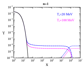
(a)

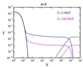
(b)

Figure 2: Evolution of co-moving number densities of $\eta_{1}$ and $N_{1}$ as a function of dimensionless variable $x$ for $\lambda_{3}=10^{-3}$, $\lambda_{\phi S}=10^{-3}$, ${M_{N_{1}}}=10$ MeV, $M_{\eta_{1}}=65$ GeV, $y_{N_{1}}=10^{-12}$, $\sin{\theta}=0.9$. Solid, dashed and dotted lines correspond to $Y_{\eta_{1}}^{eq}$, $Y_{\eta_{1}}$ and $Y_{N_{1}}$ respectively. Co-moving number densities are shown for different values of $T_{r}$ in panel $(a)$ for $n=1$, and in panel $(b)$ for $n=2$.

We will first discuss the full numerical solutions to the Boltzmann equations corresponding to $Y_{\eta_{1}}$ (Eq. 8) and $Y_{N_{1}}$ (Eq. 9) respectively. For this analysis, we first implement the interactions, mass and mixings of the model in FeynRules Alloul:2013bka , that generate required CALCHEPBelyaev:2012qa model files for micrOMEGAs Belanger:2014vza to calculate thermally averaged cross-section $<\sigma v>_{\rm eff}$. To showcase the behaviour of $Y_{\eta_{1}}$ and $Y_{N_{1}}$ with temperature $T$ we consider $M_{\eta_{1}}=65$ GeV, $M_{N_{1}}=10$ MeV, $\lambda_{3}=10^{-3},\lambda_{\phi S}=10^{-3},\sin\theta=0.9$ and the Yukawa coupling $y_{N_{1}}=10^{-12}$. It is worth pointing out that those parameters are consistent with all theoretical and experimental constraints discussed earlier. We have two additional parameters $T_{r}$ and $n$ that fix the cosmological framework of our present scenario. The co-moving number densities $Y_{\eta_{1}}$ and $Y_{N_{1}}$ for $\eta_{1}$ and $N_{1}$ are plotted as a function of $x$ for $n=1$ (Fig.2$(a)$) and $n=2$ (Fig.2$(b)$) respectively.

In Fig.2$(a)$ blue and magenta lines correspond to $T_{r}$ = 20 MeV and 100 MeV, while in Fig.2$(b)$ the corresponding two colored lines represent $T_{r}=$ 5 MeV and 100 MeV respectively. From equation (16) and equation (18) one can find that in the presence of an extra contribution to the energy density of the universe, the Hubble parameter $H$ goes like $\sim T^{2}\left(T/T_{r}\right)^{n/2},~{}~{}(T>>T_{r})$ and this explains why the expansion rate of the universe increases with the increase in $n$(for $n>0$) which ultimately leads to an earlier freeze-out of $\eta_{1}$ with higher abundance. This feature of fast expanding universe is nicely evinced in both Fig.2$(a)$ and Fig.2 $(b)$, where, co-moving number densities for $\eta_{1}$ as well as $N_{1}$ are higher for $n=2$ compared to $n=1$ for a fixed $T_{r}=100$ MeV(magenta lines). It is clearly evident from Fig.2 that ${\eta_{1}}$ decouples from the thermal bath first and then decays into $N_{1}+\nu$ at some later time which basically increases the dark matter co-moving number density $Y_{N_{1}}$. Besides, one can also notice from the Fig.2 that, for a fixed $n$, $Y_{\eta_{1}}$ decreases with the increase in $T_{r}$ and this can be once again traced back to the parametric dependence of the Hubble $H$ on $T_{r}$ and $n$ as mentioned earlier. In summary, both $Y_{\eta_{1}}$ and $Y_{N_{1}}$ increase with increase in $n$ for a given $T_{r}$, while they decrease with increase in $T_{r}$ for any value of $n\geq 1$. Interestingly both these observations can be interpreted in terms of the modified Hubble parameter $H(T)$ in the fast expanding universe.

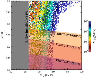
Figure 3: The allowed parameter space from the electroweak precision test (EWPT) data and Higgs’ invisible decay width constraints in ${\rm\sin{\theta}-M_{\eta_{1}}}$ plane for $10^{-6}\leq\lambda_{3}\leq 10^{-2}$, $10^{-6}\leq\lambda_{\phi S}\leq 10^{-2}$,$y_{N_{1}}=10^{-12}$ $n=2$, $T_{r}=5$ MeV. Here the color bar shows the variation of DM mass.

After illustrating the importance of the fast expanding universe in the calculation of relic abundances for both $\eta_{1}$ and $N_{1}$ we now scan the independent parameters of the model in the following range:

$$\lambda_{3}\in[10^{-6}:10^{-2}]\,,~{}\lambda_{\phi S}\in[10^{-6}:10^{-2}]$$ (20)

$$M_{\eta_{1}}\in[50~{}{\rm GeV}:100~{}{\rm GeV}]\,,M_{N_{1}}\in[1~{}{\rm MeV}:1000~{}{\rm MeV}]$$ (21)

$$\sin\theta\in[0.0:0.9]$$ (22)

The purpose of this scan is to find a region in the multi-dimensional model parameter space that is allowed by both theortical and experimental constraints as well as satisfy the correct relic density Beniwal:2020hjc ; Kannike:2012pe ; PhysRevD.46.381 ; Haber:2010bw ; ATLAS:2020kdi . We will then use those allowed parameters to calculate the value of $\Delta N_{\rm eff}$ in our model that can be substantiated in the upcoming experiments. Throughout this analysis we fix the mass of the SM-like Higgs to 125 GeV. One can notice that we vary $\sin\theta$ in the above range $(0.0-0.9)$ so that we can capture the effect of both $SU(2)$ doublet $\eta^{0}$ and singlet $S$ scalars in the freeze-in production of the DM in $\eta_{1}$ decay, where the heavy scalar $\eta_{1}$ becomes doublet (singlet) dominated for $\sin\theta=0(0.9)$. For this analysis, we fix $n=2$, $T_{r}=5$ MeV and the Yukawa coupling, $y_{N_{1}}=10^{-12}$. Varying the Yukawa coupling in the range as mentioned in section II will have no impact on relic density because

$$\Omega_{\rm DM}h^{2}=2.755\times 10^{8}\,Y_{\rm DM}\,\frac{M_{\rm DM}}{\rm GeV},$$

and $Y_{\rm DM}$ will always be same as $Y_{\eta_{1}}(x_{f.o.})$. At the end the parameter scan result in ${M_{\eta_{1}}}-\sin{\theta}$ plane is visible in Fig.3, where DM mass $M_{N_{1}}$ is represented by the color bar. As one can observe that a significant region of the parameter space in Fig.3 has been excluded by various theoretical and experimental constraints. The ${\rm Br}(h\to~{}{\rm inv})<11\%$ excludes region with $M_{\eta_{1}}<M_{h}/2$ and this is the grey coloured verical patch marked as ${\rm Br}(h\to{\rm inv})>11\%$ ATLAS:2020kdi . The electroweak precision data (EWPD) through $S,T,U$ parameters serve another crucial limit on the parameter space of this model. It is well known that larger the mass splitting between the components of $SU(2)$ doublet field, stronger is the EWPD constraints Beniwal:2020hjc . Indeed, this is happening in the case of our three benchmark points shown in Table 1. The EWPD data excludes three diagonal bands corresponding to BP-1, BP-2 and BP-3 respectively in Fig.3. From this figure, it is clear that the BP-3 which has the largest mass gap between $M_{\eta_{2}}$ and $M_{\eta^{\pm}}$ attracts the strongest EWPD limit and it excludes $\sin\theta\raise 1.29167pt\hbox{$\;<$\kern-7.5pt\raise-4.73611pt\hbox{$\sim\;$}}0.6-0.775$ for $M_{\eta_{1}}\approx 62.5$ GeV and $\sin\theta\raise 1.29167pt\hbox{$\;<$\kern-7.5pt\raise-4.73611pt\hbox{$\sim\;$}}0.6-0.75$ for $M_{\eta_{1}}=100$ GeV. Thus, the overall allowed region is located at the upper quadrilateral part of the parameter space, with $\sin\theta\sim 0.775-0.9$ and $M_{\eta_{1}}\sim 62.5~{}{\rm GeV}-100~{}{\rm GeV}$. Another important outcome of our analysis is that for a fixed $\sin\theta$ any increase in $M_{N_{1}}$, also call for an increase in $M_{\eta_{1}}$ to satisfy the correct density and Fig.3 perfectly corroborate our claim. However, one has to look for any physical processes that may imperil the effect of long-lived scalar on cosmic microwave background (CMB) in singlet-doublet scotogenic model. In this scenario, the presence of other heavy scalars may lead to DM co-annihilation processes which may boost the $\left<\sigma v\right>_{\rm eff}$ and such enhanced $\left<\sigma v\right>_{\rm eff}$ ultimately suppress $\eta_{1}$ abundance. The immediate consequence of this low yield $\eta_{1}$ is the tiny production of additional neutrino density $\rho^{\prime}_{\nu}$ that may not lead to any significant shift in $\Delta N_{\rm eff}$, thus spoiling the intention of this analysis. The most natural way to circumvent this situation, is to take other particles of the model very heavy compared to $M_{\eta_{1}}$ (large mass splittings) so that one can easily ignore the co-annihilation of $\eta_{1}$ with those heavier particles. To facilitate this in our analysis we choose three representative benchmark points (BP-1, BP-2 & BP-3) as shown in Table 1.

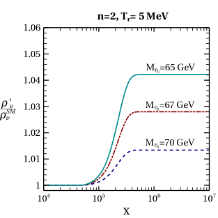
(a)

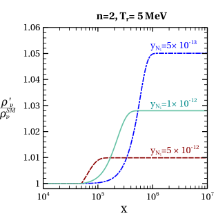
(b)

Figure 4: Evolution of the ratio $\rm{\rho_{\nu}^{\prime}/\rho_{\nu}^{SM}}$ as a function of $x$ for $\lambda_{3}=10^{-3}$, $\lambda_{\phi S}=10^{-3}$, ${M_{N_{1}}}=10$ MeV, $\sin{\theta}=0.9$, $n=2$, $T_{r}=5$ MeV. We show our findings for three different values of $\rm{M_{\eta_{1}}}$ for a fixed $y_{N_{1}}=10^{-12}$ in Fig. 4(a) and for three different values of $y_{N_{1}}$ for constant $\rm{M_{\eta_{1}}}=67$ GeV in Fig. 4(b).

After having a suitable model parameter space consistent with various constraints, we are now in a position to kickoff the numerical estimation of the ratio ${\rho_{\nu}^{\prime}}/{\rho_{\nu}^{SM}}$. For this we need to solve equation (8) and (13) to evaluate the evolution of ${\rho_{\nu}^{\prime}}/{\rho_{\nu}^{SM}}$ as a function of the dimensionless variable $x$. In Fig.4(a) we display the dependence of ${\rho_{\nu}^{\prime}}/{\rho_{\nu}^{SM}}$ as a function of $x$ for three different values of ${M_{\eta_{1}}}$ (65 GeV (solid cyan line), 67 GeV (brown dot dashed line), 70 GeV (blue dashed line) where the other parameters are kept fixed ($\lambda_{3}=10^{-3}$, $\lambda_{\phi S}=10^{-3}$, ${M_{N_{1}}}=10$ MeV, $\sin{\theta}=0.9$, $n=2$, $T_{r}=5$ MeV) for a constant Yukawa coupling $y_{N_{1}}=10^{-12}$. From this figure (Fig.4(a)) one can clearly discern that at very high temperature $T$, $\eta_{1}$ stays in thermal equilibrium for $M_{\eta_{1}}=65$ GeV and with no additional contribution to $\rho^{\prime}_{\nu}$ from $\eta_{1}$, thus the ratio ${\rho_{\nu}^{\prime}}/{\rho_{\nu}^{SM}}$ is almost unity. However, as the universe starts cooling, the decay $\eta_{1}\to N_{1}+\nu$ also proceeds through tiny Yukawa coupling $y_{N_{1}}$ and it leads to new contributions to the neutrino energy density. This additional contribution makes the ratio ${\rho_{\nu}^{\prime}}/{\rho_{\nu}^{SM}}$ greater than one. The decay of $\eta_{1}$ continues until its number density is completely converted into $N_{1}$ and $\nu$ number densities. At that point, no further neutrinos are generated and the ${\rho_{\nu}^{\prime}}/{\rho_{\nu}^{SM}}$ saturates. This feature is repeated for other two values of $M_{\eta_{1}}=67$ GeV and $70$ GeV in Fig. 4(a) with a marked difference. For higher value of $M_{\eta_{1}}$ the thermally averaged cross-section $(\left<\sigma v\right>)_{\rm eff}$ of $\eta_{1}$ with SM particles increases due to larger phase space availability. This elevated cross-section leads to the late time freeze out of $\eta_{1}$ with smaller abundance. Subsequently the late time decay of $\eta_{1}$ produces neutrinos with suppressed energy density Beniwal:2020hjc . From this analysis we conclude that for a fixed value of $x$, the ratio ${\rho_{\nu}^{\prime}}/{\rho_{\nu}^{SM}}$ is the largest (smallest) for $M_{\eta_{1}}=65(70)$ GeV respectively.

The Yukawa coupling $y_{N_{1}}$ also controls the temperature $T$ variation of the ratio ${\rho_{\nu}^{\prime}}/{\rho_{\nu}^{SM}}$ for a fixed $\eta_{1}$ mass. In Fig.4(b), we show such variation of ${\rho_{\nu}^{\prime}}/{\rho_{\nu}^{SM}}$ with $x$ assuming three different values of $y_{N_{1}}$ ($5\times 10^{-12}$ (brown dashed line), $1\times 10^{-12}$(solid cyan line ), $5\times 10^{-13}$ (blue dot dashed line) for $M_{\eta_{1}}=67$ GeV, while other parameters are same as in Fig.4(a). For a given mass of $\eta_{1}$ and $N_{1}$ and keeping other model parameters fixed, the decay of $\eta_{1}\to N_{1}+\nu$ is completely determined by the Yukawa coupling $y_{N_{1}}$. Besides, larger the coupling $y_{N_{1}}$, faster is the decay rate of $\eta_{1}$ and vice-versa. For a given $y_{N_{1}}$, the ratio keeps on increasing with the expansion of the universe and ultimately saturates when the decay of $\eta_{1}$ is completed. For any higher $y_{N_{1}}$, the aforementioned decay of $\eta_{1}$ gets completed even at earlier time (equivalently at higher temperature $T$) and the energy injection to neutrino sector also completes at earlier epoch of the universe. This phenomena is distinctly noticeable from Fig.4(b) that the ratio saturates earlier with increase in $y_{N_{1}}$. As the higher value of Yukawa coupling forces the $\eta_{1}$ decay to be completed at earlier time, the new contribution to neutrino energy density $\rm{\rho_{\nu}^{\prime}}$ from this decay gets diluted more due to the expansion of the universe. However with lower Yukawa coupling $y_{N_{1}}=5\times 10^{-13}$, the decay starts later and the corresponding energy injection to neutrino sector also gets completed at later time (lower temperature) hence gets less diluted due to the expansion of the universe. Consequently, one gets a higher value of ${\rho_{\nu}^{\prime}}/{\rho_{\nu}^{SM}}$ at lower temperature ($x\approx 10^{7}$) as depicted in Fig. 4(b).

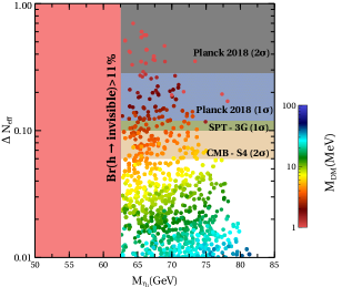
Figure 5: Variation of ${\rm\Delta N_{eff}}$ with $M_{\eta_{1}}$ for ${M_{A^{0}}}=250$ GeV, ${M_{\eta^{+}}}=180$ GeV, ${M_{\eta_{2}}}=400$ GeV, $10^{-6}\leq\lambda_{3}\leq 10^{-2}$, $10^{-6}\leq\lambda_{\phi S}\leq 10^{-2}$,$y_{N_{1}}=10^{-12}$ and $n=2$, $T_{r}=5$ MeV. The color bar in the plot represents the DM mass.

After highlighting the variation of ${\rho_{\nu}^{\prime}}/{\rho_{\nu}^{SM}}$ with various model parameters, we now use ${\rho_{\nu}^{\prime}}/{\rho_{\nu}^{SM}}$ to calculate the $\rm{\Delta N_{eff}}$ by scanning over those model parameters and the corresponding upshot is displayed in $\Delta N_{\rm eff}$ vs $M_{\eta_{1}}$ plane in Fig.5. The color bar represents the value of $\rm{M_{N_{1}}}$ in the range $1~{}{\rm MeV}-100~{}{\rm MeV}$. Here we consider BP-1 as the maximum allowed region from EWPD constraints correspond to this particular benchmark point. Similarly other parameter space points satisfy the correct relic density as well as are consistent with other theoretical and experimental constraints. In the calculation of $\Delta N_{\rm eff}$, we vary the DM mass $M_{N_{1}}$ from $1$ MeV to $100$ MeV and it is conspicuous from Fig.5, that with increase in $M_{N_{1}}$, the numerical value of $\rm{\Delta N_{eff}}$ decreases. This is understandable as a higher value of $M_{N_{1}}$ requires lower abundance $Y_{N_{1}}$ so that the correct relic density($\Omega h^{2}\sim Y_{N_{1}}M_{N_{1}}$) is achieved. In our earlier discussions, we have shown that the evolution of $N_{1}$ abundance is governed by $Y_{\eta_{1}}$(Fig. 2(a)), thus, lower $Y_{N_{1}}$ also corresponds to smaller $\eta_{1}$ abundance $Y_{\eta_{1}}$. With this lower abundance of $\eta_{1}$ lesser energy gets transferred to neutrino sector, leading to smaller value of $\rm{\Delta N_{eff}}$. For this scan we consider fixed $y_{N_{1}}=10^{-12}$. We may decrease $y_{N_{1}}$ that would lead an increase in $\rm{\Delta N_{eff}}$ as understood from Fig.4(b), and will make the scenario more viable to the observations. However the DM phenomenology will remain same. We also show the exclusion limit of $\rm{\Delta N_{eff}}$ from different present and future generation experiments. The present $2\sigma$ limit from Planck(2018) on ${\rm\Delta N_{eff}=0.285}$ excludes the DM mass between $\sim 1$ and $2$ MeV. Whereas the 1$\sigma$ limit from Planck(2018) on ${\rm\Delta N_{eff}=0.12}$ excludes DM mass in the range $\sim 3-4$ MeV. It is also important to note that the future generation experiments such as the SPT-3GSPT-3G:2019sok with 1$\sigma$ limit on $\Delta N_{\rm eff}=0.1$ and the CMB-S4CMB-S4:2016ple with 2$\sigma$ limit on $\Delta N_{\rm eff}=0.06$ will be able to probe the DM mass upto $\sim 7$ MeV and $\sim 10$ MeV respectively. Hence with the present and future generation experimental measurement of $\Delta N_{\rm eff}$ we can indirectly probe the freeze-in DM in this scenario and also rule out certain mass range of such feebly interacting dark matter.

V Summary and Conclusion

We have discussed a minimal extension of the SM by an inert $SU(2)_{L}$ scalar doublet $(\eta)$, a real scalar singlet $(S)$ and three right handed singlet fermions $(N_{1},N_{2},\&N_{3})$ where all of them are odd under $\mathcal{Z}_{2}$ symmetry. However, the SM particles are even under the above-mentioned $\mathcal{Z}_{2}$ symmetry. The study has been restricted to the regime where $M_{N_{1}}$ is lightest new particle in the spectrum and play the role of a stable DM candidate. Due to the chosen $\mathcal{Z}_{2}$ symmetry, $N_{i}$s can only interact with SM particles through the yukawa interaction with $\eta$ and SM lepton doublet. We have assumed that the interaction of $N_{1}$ is very feeble which is decided by the Yukawa coupling $(y_{N_{1}}\lesssim 10^{-12})$. Such a small interaction of $N_{1}$ prevents its production in the thermal bath. Rather, ${N_{1}}$ has been produced from the non-thermal decay of long lived lightest scalar $\eta_{1}$, which is one of the neutral CP even scalar mass eigen state obtained by diagonalizing the $2\times 2$ mass-square matrix in $(\eta^{0},S)$ basis. The masses of all the other $\mathcal{Z}_{2}$ odd particles is sufficiently large and have no phenomenological consequences in the DM analysis. The SM neutrino masses can be generated through one loop process via interactions of $N_{i}$ and $\eta_{1}$ with the SM leptons. However, with such tiny Yukawa interaction ${N_{1}}$ is almost decoupled from the neutrino mass generation and as a result one of the active neutrino becomes almost massless. We have first checked the effects of different model parameters on the relic density of DM by solving the required Boltzmann equations. We have found that constraints coming from the electroweak precision data as well as the invisible decay of the SM Higgs boson ruled out a significant fraction of the model parameter space. We have seen that in the standard radiation dominated universe, the number densities of the mother particles $(\eta_{1})$ which have sizable interactions with the SM bath becomes smaller and have negligible impact on the $\Delta{N_{\rm eff}}$. On the other hand, if the early epoch of the expansion was dominated by some non-standard species that can chage the outcome by causing faster expansion of the universe. In this fast expanding universe scenario apart from producing the right amount of DM relic density, the late time decay of $\eta_{1}$ can significantly impact the total radiation energy density on the start of CMB formation and puts further constraints to the allowed parameter space of the model. In order to calculate the amount of ${\rm\Delta N_{eff}}$, we have found out the of the amount of energy density of neutrinos coming from the decay of $\eta_{1}$ by solving the required Boltzmann equation. The present $2\sigma$ limit on ${\rm\Delta N_{eff}}$ from Planck 2018 data excludes the DM mass as heavy as 2 MeV as in case of lighter DM mass, more and more energy gets converted to neutrinos and increases the value of ${\rm\Delta{N_{eff}}}$. However, the future generation experiments like SPT-3G, CMB-IV will be able to probe the dark matter mass as heavy as $\sim 10$ MeV. Thus the analysis performed in this paper can be considered as an alternative way to probe the FIMP dark matter scenario by the precise determination of $\Delta N_{\rm eff}$ using the current and future CMB data.

VI Acknowledgements

DN and SJ would like to thank D. Borah, A. Biswas, K. Dutta, S. Ganguly, D. Ghosh and Md. I. Ali for various discussions during the project. The work of DN is partly supported by National Research Foundation of Korea (NRF)’s grants, grants no. 2019R1A2C3005009(DN). The work of SJ is supported by CSIR, Government of India, under the NET JRF fellowship scheme with Award file No. 09/080(1172)/2020-EMR-I.

Appendix A Particle contents and the model parameters

Particle content is given by

	$SU(2)_{L}$	$U(1)_{Y}$	$Z_{2}$
$\phi$	2	$\frac{1}{2}$	+
$\eta$	2	$\frac{1}{2}$	-
S	1	0	-

The scalar potential $V(\phi,\eta,S)$ is :

$$V(\phi,\eta,S) = -\mu_{\phi}^{2}(\phi^{\dagger}\phi)+\mu_{\eta}^{2}(\eta^{\dagger}\eta)+\lambda_{1}(\phi^{\dagger}\phi)^{2}+\lambda_{2}(\eta^{\dagger}\eta)^{2}+\mu_{s}^{2}S^{2}+\lambda_{s}S^{4}$$ (23)

$$+\lambda_{3}(\phi^{\dagger}\phi)(\eta^{\dagger}\eta)+\lambda_{4}(\phi^{\dagger}\eta)(\eta^{\dagger}\phi)+\frac{\lambda_{5}}{2}\left\{(\phi^{\dagger}\eta)^{2}+(\eta^{\dagger}\phi)^{2}\right\}$$

$$+\lambda_{\phi S}(\phi^{\dagger}\phi)S^{2}+\lambda_{\eta S}(\eta^{\dagger}\eta)S^{2}+\mu^{\prime}\left\{(\phi^{\dagger}\eta)S+(\eta^{\dagger}\phi)S\right\},$$

where all parameters are real and $\mu_{i(i=\phi,\eta,s)}$ are the bare mass terms, $\mu^{\prime}$ is the trilinear scalar coupling, while various quartic scalar couplings are represented by $\lambda_{i(i=1-5)},\lambda_{\phi S}$ and $\lambda_{\eta S}$ respectively. We write the SM scalar doublet as

$$\phi=\dfrac{1}{\sqrt{2}}\begin{bmatrix}&\phi_{1}+i\,\phi_{2}\\ &\phi_{3}+i\,\phi_{4}\end{bmatrix}\,$$ (24)

where $\phi_{i}$ are real. From the minimization condition of the potential $V$ in equation (23) we get:

$$\phi_{j}\left(-\mu_{\phi}^{2}+\lambda_{1}\sum_{i}^{4}\phi_{i}^{2}\right)=0$$ (25)

Any point on the circle $\left(-\mu_{\phi}^{2}+\lambda_{1}\sum_{i}^{4}\phi^{2}\right)=0$ is a local minimum of the potential in equation (23) and choosing a particular point ($\phi_{1}=\phi_{2}=\phi_{4}=0,\phi_{3}=v=\sqrt{\mu_{\phi}^{2}/\lambda_{1}}$) will spontaneously break the symmetry. After the spontaneous symmetry breaking of the SM higgs doublet the doublet scalars can be represented as follows:

$$\phi=\begin{bmatrix}&0\\ &\dfrac{v+h}{\sqrt{2}}\end{bmatrix}\,,\eta=\begin{bmatrix}&\eta^{\pm}\\ &\dfrac{\eta^{0}+i\,A^{0}}{\sqrt{2}}\end{bmatrix},$$ (26)

where, $v=246$ GeV, is the SM electroweak vacuum expectation value (vev). The masses of the SM like Higgs ($h$) and the charged scalar($\eta^{\pm}$) and the pseudo scalar particles($A^{0}$) can be written as ,

$$M_{h}^{2} = 2\lambda_{1}v^{2}$$ (27)

$$M^{2}_{\eta^{\pm}} = \mu_{\eta}^{2}+\dfrac{\lambda_{3}}{2}v^{2}$$ (28)

$$M^{2}_{A^{0}} = \mu_{\eta}^{2}+(\lambda_{3}+\lambda_{4}-\lambda_{5})\dfrac{v^{2}}{2}$$ (29)

Due to the presence of the trilinear interaction $(\phi^{\dagger}\eta\,S)$ in the scalar potential, the neutral CP even component $\eta^{0}$ mixes with the real singlet scalar $S$ and the corresponding mass-square matrix in ($\eta^{0}$, $S$) basis has the following form:

$$M_{\eta^{0}S}^{2}=\begin{bmatrix}&\frac{\partial^{2}V}{\partial{\eta^{0}}^{2}}&\frac{\partial^{2}V}{\partial{\eta^{0}}\partial S}\\ &\frac{\partial^{2}V}{\partial{\eta^{0}}\partial S}&\frac{\partial^{2}V}{\partial S^{2}}\end{bmatrix}=\begin{bmatrix}&\mu_{\eta}^{2}+\lambda_{L}v^{2}&v\ \mu^{\prime}\\ &v\ \mu^{\prime}&2\mu_{s}^{2}+\lambda_{\phi S}\ v^{2}\end{bmatrix},$$ (30)

where, $\lambda_{L}=\frac{1}{2}(\lambda_{3}+\lambda_{4}+\lambda_{5})$. The eigen values and CP-even neutral physical eigen states can be obtained by digonalising the above mass squared matrix:

$$M^{2}_{\eta_{1}\eta_{2}}=O^{T}M_{\eta^{0}S}^{2}O,$$ (31)

where

$$O=\begin{bmatrix}\cos\theta&\sin{\theta}\\ -\sin{\theta}&\cos{\theta}\end{bmatrix},$$ (32)

and $M^{2}_{\eta_{1}\eta_{2}}$ is given by,

$$M^{2}_{\eta_{1}\eta_{2}}=\begin{bmatrix}&M^{2}_{\eta_{1}}&0\\ &0&M^{2}_{\eta_{2}}.\end{bmatrix}$$ (33)

The corresponding eigen states $\eta_{1}$ and $\eta_{2}$ are given in terms of the weak basis $(\eta^{0},S)$ and the mixing angle $\theta$:

$$\eta_{1} = \eta^{0}\cos\theta-S\sin\theta$$ (34)

$$\eta_{2} = \eta^{0}\sin\theta+S\cos\theta$$ (35)

The free parameters of the scalar sectors are the following: $M_{\eta_{1}}$, $M_{\eta_{2}}$, $M_{\eta^{\pm}}$, $M_{A^{0}}$, $\lambda_{\eta}$, $\lambda_{S}$, $\lambda_{\phi S}$, $\lambda_{\eta S}$, $\lambda_{3}$, and $\sin\theta$. We set the SM like Higgs boson mass, $M_{h}=125$ GeV through out this analysis. All other parameters of the scalar sector can be expressed in terms of those free parameters. From equations (30-33) we get the following relations:

$$\mu_{\eta}^{2} = \cos^{2}{\theta}\,M^{2}_{\eta_{1}}+\sin^{2}{\theta}\,M^{2}_{\eta_{2}}-\lambda_{L}v^{2}$$ (36)

$$\mu^{\prime} = \cos{\theta}\ \sin{\theta}\,\frac{1}{v}\left(M^{2}_{\eta_{2}}-M^{2}_{\eta_{1}}\right)$$ (37)

$$\mu_{s}^{2} = \frac{1}{2}(\sin^{2}{\theta}\,M^{2}_{\eta_{1}}+\cos^{2}{\theta}\,M^{2}_{\eta_{2}}-\lambda_{\phi S}\ v^{2})$$ (38)

Substituting these parameters in scalar masses in equation (29) we get,

$$\lambda_{5} = \frac{1}{v^{2}}\left(\cos^{2}{\theta}\ M^{2}_{\eta_{1}}+\sin^{2}{\theta}\ M^{2}_{\eta_{2}}-M_{A^{0}}^{2}\right)$$ (39)

$$\lambda_{4}+\lambda_{5} = \frac{2}{v^{2}}\left(\cos^{2}{\theta}M_{\eta_{1}}^{2}+\sin^{2}{\theta}M_{\eta_{2}}^{2}-M_{\eta^{+}}^{2}\right)$$ (40)

Now we have written the dependent parameters ($\mu_{\eta}\,,\mu^{\prime}\,,\mu_{S}\,,\lambda_{4}\,,\lambda_{5}$) in terms of free parameters.

References

- (1) T2K collaboration, Indication of Electron Neutrino Appearance from an Accelerator-produced Off-axis Muon Neutrino Beam, Phys. Rev. Lett. 107 (2011) 041801 [1106.2822].
- (2) Double Chooz collaboration, Indication of Reactor Disappearance in the Double Chooz Experiment, Phys. Rev. Lett. 108 (2012) 131801 [1112.6353].
- (3) Daya Bay collaboration, Observation of electron-antineutrino disappearance at Daya Bay, Phys. Rev. Lett. 108 (2012) 171803 [1203.1669].
- (4) RENO collaboration, Observation of Reactor Electron Antineutrino Disappearance in the RENO Experiment, Phys. Rev. Lett. 108 (2012) 191802 [1204.0626].
- (5) MINOS collaboration, Electron neutrino and antineutrino appearance in the full MINOS data sample, Phys. Rev. Lett. 110 (2013) 171801 [1301.4581].
- (6) Particle Data Group collaboration, Review of Particle Physics, PTEP 2020 (2020) 083C01.
- (7) F. Zwicky, Die Rotverschiebung von extragalaktischen Nebeln, Helv. Phys. Acta 6 (1933) 110.
- (8) V.C. Rubin and W.K. Ford, Jr., Rotation of the Andromeda Nebula from a Spectroscopic Survey of Emission Regions, Astrophys. J. 159 (1970) 379.
- (9) D. Clowe, M. Bradac, A.H. Gonzalez, M. Markevitch, S.W. Randall, C. Jones et al., A direct empirical proof of the existence of dark matter, Astrophys. J. Lett. 648 (2006) L109 [astro-ph/0608407].
- (10) Planck collaboration, Planck 2018 results. VI. Cosmological parameters, Astron. Astrophys. 641 (2020) A6 [1807.06209].
- (11) P. Minkowski, at a Rate of One Out of Muon Decays?, Phys. Lett. B 67 (1977) 421.
- (12) R.N. Mohapatra and G. Senjanovic, Neutrino Mass and Spontaneous Parity Nonconservation, Phys. Rev. Lett. 44 (1980) 912.
- (13) J. Schechter and J.W.F. Valle, Neutrino Masses in SU(2) x U(1) Theories, Phys. Rev. D 22 (1980) 2227.
- (14) M. Gell-Mann, P. Ramond and R. Slansky, Complex Spinors and Unified Theories, Conf. Proc. C 790927 (1979) 315 [1306.4669].
- (15) R.N. Mohapatra and G. Senjanovic, Neutrino Masses and Mixings in Gauge Models with Spontaneous Parity Violation, Phys. Rev. D 23 (1981) 165.
- (16) G. Lazarides, Q. Shafi and C. Wetterich, Proton Lifetime and Fermion Masses in an SO(10) Model, Nucl. Phys. B 181 (1981) 287.
- (17) C. Wetterich, Neutrino Masses and the Scale of B-L Violation, Nucl. Phys. B 187 (1981) 343.
- (18) J. Schechter and J.W.F. Valle, Neutrino Decay and Spontaneous Violation of Lepton Number, Phys. Rev. D 25 (1982) 774.
- (19) B. Brahmachari and R.N. Mohapatra, Unified explanation of the solar and atmospheric neutrino puzzles in a minimal supersymmetric SO(10) model, Phys. Rev. D 58 (1998) 015001 [hep-ph/9710371].
- (20) R. Foot, H. Lew, X.G. He and G.C. Joshi, Seesaw Neutrino Masses Induced by a Triplet of Leptons, Z. Phys. C 44 (1989) 441.
- (21) E. Ma, Pathways to naturally small neutrino masses, Phys. Rev. Lett. 81 (1998) 1171 [hep-ph/9805219].
- (22) E. Ma, Verifiable radiative seesaw mechanism of neutrino mass and dark matter, Phys. Rev. D 73 (2006) 077301 [hep-ph/0601225].
- (23) E.W. Kolb and M.S. Turner, The Early Universe, vol. 69 (1990), 10.1201/9780429492860.
- (24) J.L. Feng, Dark Matter Candidates from Particle Physics and Methods of Detection, Ann. Rev. Astron. Astrophys. 48 (2010) 495 [1003.0904].
- (25) L. Roszkowski, E.M. Sessolo and S. Trojanowski, WIMP dark matter candidates and searches—current status and future prospects, Rept. Prog. Phys. 81 (2018) 066201 [1707.06277].
- (26) M. Schumann, Direct Detection of WIMP Dark Matter: Concepts and Status, J. Phys. G 46 (2019) 103003 [1903.03026].
- (27) T. Lin, Dark matter models and direct detection, PoS 333 (2019) 009 [1904.07915].
- (28) G. Arcadi, M. Dutra, P. Ghosh, M. Lindner, Y. Mambrini, M. Pierre et al., The waning of the WIMP? A review of models, searches, and constraints, Eur. Phys. J. C 78 (2018) 203 [1703.07364].
- (29) PandaX-II collaboration, Dark Matter Results from First 98.7 Days of Data from the PandaX-II Experiment, Phys. Rev. Lett. 117 (2016) 121303 [1607.07400].
- (30) XENON collaboration, First Dark Matter Search Results from the XENON1T Experiment, Phys. Rev. Lett. 119 (2017) 181301 [1705.06655].
- (31) LUX collaboration, Results from a search for dark matter in the complete LUX exposure, Phys. Rev. Lett. 118 (2017) 021303 [1608.07648].
- (32) PICO collaboration, Dark Matter Search Results from the Complete Exposure of the PICO-60 C3F8 Bubble Chamber, Phys. Rev. D 100 (2019) 022001 [1902.04031].
- (33) AMS collaboration, First Result from the Alpha Magnetic Spectrometer on the International Space Station: Precision Measurement of the Positron Fraction in Primary Cosmic Rays of 0.5–350 GeV, Phys. Rev. Lett. 110 (2013) 141102.
- (34) J. Buckley et al., Working Group Report: WIMP Dark Matter Indirect Detection, in Community Summer Study 2013: Snowmass on the Mississippi, 10, 2013 [1310.7040].
- (35) J.M. Gaskins, A review of indirect searches for particle dark matter, Contemp. Phys. 57 (2016) 496 [1604.00014].
- (36) Fermi-LAT, DES collaboration, Searching for Dark Matter Annihilation in Recently Discovered Milky Way Satellites with Fermi-LAT, Astrophys. J. 834 (2017) 110 [1611.03184].
- (37) MAGIC, Fermi-LAT collaboration, Limits to Dark Matter Annihilation Cross-Section from a Combined Analysis of MAGIC and Fermi-LAT Observations of Dwarf Satellite Galaxies, JCAP 02 (2016) 039 [1601.06590].
- (38) T. Bringmann and C. Weniger, Gamma Ray Signals from Dark Matter: Concepts, Status and Prospects, Phys. Dark Univ. 1 (2012) 194 [1208.5481].
- (39) M. Cirelli, Status of Indirect (and Direct) Dark Matter searches, PoS ICRC2015 (2016) 014 [1511.02031].
- (40) F. Kahlhoefer, Review of LHC Dark Matter Searches, Int. J. Mod. Phys. A 32 (2017) 1730006 [1702.02430].
- (41) A. Boveia and C. Doglioni, Dark Matter Searches at Colliders, Ann. Rev. Nucl. Part. Sci. 68 (2018) 429 [1810.12238].
- (42) L.J. Hall, K. Jedamzik, J. March-Russell and S.M. West, Freeze-In Production of FIMP Dark Matter, JHEP 03 (2010) 080 [0911.1120].
- (43) J. König, A. Merle and M. Totzauer, keV Sterile Neutrino Dark Matter from Singlet Scalar Decays: The Most General Case, JCAP 11 (2016) 038 [1609.01289].
- (44) A. Biswas and A. Gupta, Freeze-in Production of Sterile Neutrino Dark Matter in U(1)B-L Model, JCAP 09 (2016) 044 [1607.01469].
- (45) A. Biswas and A. Gupta, Calculation of Momentum Distribution Function of a Non-thermal Fermionic Dark Matter, JCAP 03 (2017) 033 [1612.02793].
- (46) N. Bernal, M. Heikinheimo, T. Tenkanen, K. Tuominen and V. Vaskonen, The Dawn of FIMP Dark Matter: A Review of Models and Constraints, Int. J. Mod. Phys. A 32 (2017) 1730023 [1706.07442].
- (47) D. Borah, B. Karmakar and D. Nanda, Common Origin of Dirac Neutrino Mass and Freeze-in Massive Particle Dark Matter, JCAP 07 (2018) 039 [1805.11115].
- (48) J. Heeck and D. Teresi, Cold keV dark matter from decays and scatterings, Phys. Rev. D 96 (2017) 035018 [1706.09909].
- (49) K.J. Bae, A. Kamada, S.P. Liew and K. Yanagi, Light axinos from freeze-in: production processes, phase space distributions, and Ly- forest constraints, JCAP 01 (2018) 054 [1707.06418].
- (50) S. Boulebnane, J. Heeck, A. Nguyen and D. Teresi, Cold light dark matter in extended seesaw models, JCAP 04 (2018) 006 [1709.07283].
- (51) G. Ballesteros, M.A.G. Garcia and M. Pierre, How warm are non-thermal relics? Lyman- bounds on out-of-equilibrium dark matter, JCAP 03 (2021) 101 [2011.13458].
- (52) F. D’Eramo and A. Lenoci, Lower mass bounds on FIMP dark matter produced via freeze-in, JCAP 10 (2021) 045 [2012.01446].
- (53) Q. Decant, J. Heisig, D.C. Hooper and L. Lopez-Honorez, Lyman- constraints on freeze-in and superWIMPs, JCAP 03 (2022) 041 [2111.09321].
- (54) S.-P. Li, X.-Q. Li, X.-S. Yan and Y.-D. Yang, Simple estimate of BBN sensitivity to light freeze-in dark matter, Phys. Rev. D 104 (2021) 115007 [2106.07122].
- (55) S. Ganguly, S. Roy and A.K. Saha, Imprints of MeV Scale Hidden Dark Sector at Planck, 2201.00854.
- (56) G. Mangano, G. Miele, S. Pastor, T. Pinto, O. Pisanti and P.D. Serpico, Relic neutrino decoupling including flavor oscillations, Nucl. Phys. B 729 (2005) 221 [hep-ph/0506164].
- (57) E. Grohs, G.M. Fuller, C.T. Kishimoto, M.W. Paris and A. Vlasenko, Neutrino energy transport in weak decoupling and big bang nucleosynthesis, Phys. Rev. D 93 (2016) 083522 [1512.02205].
- (58) P.F. de Salas and S. Pastor, Relic neutrino decoupling with flavour oscillations revisited, JCAP 07 (2016) 051 [1606.06986].
- (59) SPT-3G collaboration, Particle Physics with the Cosmic Microwave Background with SPT-3G, J. Phys. Conf. Ser. 1468 (2020) 012008 [1911.08047].
- (60) CMB-S4 collaboration, CMB-S4 Science Book, First Edition, 1610.02743.
- (61) M. Kawasaki, K. Kohri and N. Sugiyama, MeV scale reheating temperature and thermalization of neutrino background, Phys. Rev. D 62 (2000) 023506 [astro-ph/0002127].
- (62) K. Ichikawa, M. Kawasaki and F. Takahashi, The Oscillation effects on thermalization of the neutrinos in the Universe with low reheating temperature, Phys. Rev. D 72 (2005) 043522 [astro-ph/0505395].
- (63) F. D’Eramo, N. Fernandez and S. Profumo, When the Universe Expands Too Fast: Relentless Dark Matter, JCAP 05 (2017) 012 [1703.04793].
- (64) M. Joyce, Electroweak baryogenesis and the expansion rate of the universe, Phys. Rev. D 55 (1997) 1875.
- (65) M.S. Turner, Coherent scalar-field oscillations in an expanding universe, Phys. Rev. D 28 (1983) 1243.
- (66) D. Wands, E. COPELAND and A. Liddle, Exponential potentials, scaling solutions and inflation, Annals of the New York Academy of Sciences 688 (2006) 647 .
- (67) B. Ratra and P.J.E. Peebles, Cosmological consequences of a rolling homogeneous scalar field, Phys. Rev. D 37 (1988) 3406.
- (68) E.J. Copeland, A.R. Liddle and D. Wands, Exponential potentials and cosmological scaling solutions, Phys. Rev. D 57 (1998) 4686 [gr-qc/9711068].
- (69) N. Bernal, C. Cosme, T. Tenkanen and V. Vaskonen, Scalar singlet dark matter in non-standard cosmologies, Eur. Phys. J. C 79 (2019) 30 [1806.11122].
- (70) A. Poulin, Dark matter freeze-out in modified cosmological scenarios, Phys. Rev. D 100 (2019) 043022 [1905.03126].
- (71) K. Redmond and A.L. Erickcek, New Constraints on Dark Matter Production during Kination, Phys. Rev. D 96 (2017) 043511 [1704.01056].
- (72) E. Hardy, Higgs portal dark matter in non-standard cosmological histories, JHEP 06 (2018) 043 [1804.06783].
- (73) B. Barman, P. Ghosh, F.S. Queiroz and A.K. Saha, Scalar multiplet dark matter in a fast expanding Universe: Resurrection of the desert region, Phys. Rev. D 104 (2021) 015040 [2101.10175].
- (74) F. D’Eramo, N. Fernandez and S. Profumo, Dark Matter Freeze-in Production in Fast-Expanding Universes, JCAP 02 (2018) 046 [1712.07453].
- (75) R.T. Co, F. D’Eramo, L.J. Hall and D. Pappadopulo, Freeze-In Dark Matter with Displaced Signatures at Colliders, JCAP 12 (2015) 024 [1506.07532].
- (76) A. Berlin, D. Hooper and G. Krnjaic, PeV-Scale Dark Matter as a Thermal Relic of a Decoupled Sector, Phys. Lett. B 760 (2016) 106 [1602.08490].
- (77) T. Tenkanen and V. Vaskonen, Reheating the Standard Model from a hidden sector, Phys. Rev. D 94 (2016) 083516 [1606.00192].
- (78) J.A. Dror, E. Kuflik and W.H. Ng, Codecaying Dark Matter, Phys. Rev. Lett. 117 (2016) 211801 [1607.03110].
- (79) A. Berlin, D. Hooper and G. Krnjaic, Thermal Dark Matter From A Highly Decoupled Sector, Phys. Rev. D 94 (2016) 095019 [1609.02555].
- (80) D. Borah, P.S.B. Dev and A. Kumar, TeV scale leptogenesis, inflaton dark matter and neutrino mass in a scotogenic model, Phys. Rev. D 99 (2019) 055012 [1810.03645].
- (81) T. Kitabayashi, Primordial black holes and scotogenic dark matter, Int. J. Mod. Phys. A 36 (2021) 2150139 [2101.01921].
- (82) V. De Romeri, M. Puerta and A. Vicente, Dark matter in a charged variant of the Scotogenic model, 2106.00481.
- (83) P. Escribano and A. Vicente, An ultraviolet completion for the Scotogenic model, Phys. Lett. B 823 (2021) 136717 [2107.10265].
- (84) I.M. Ávila, G. Cottin and M.A. Díaz, Revisiting the scotogenic model with scalar dark matter, 2108.05103.
- (85) A. Alvarez, R. Cepedello, M. Hirsch and W. Porod, Temperature effects on the Z2 symmetry breaking in the scotogenic model, Phys. Rev. D 105 (2022) 035013 [2110.04311].
- (86) P. Escribano, A generalization of the Scotogenic model, 10, 2021 [2110.07890].
- (87) R.S. Hundi, Lepton flavor violating and Higgs decays in the scotogenic model, 2201.03779.
- (88) N.G. Deshpande and E. Ma, Pattern of Symmetry Breaking with Two Higgs Doublets, Phys. Rev. D 18 (1978) 2574.
- (89) R. Barbieri, L.J. Hall and V.S. Rychkov, Improved naturalness with a heavy Higgs: An Alternative road to LHC physics, Phys. Rev. D 74 (2006) 015007 [hep-ph/0603188].
- (90) L. Lopez Honorez, E. Nezri, J.F. Oliver and M.H.G. Tytgat, The Inert Doublet Model: An Archetype for Dark Matter, JCAP 02 (2007) 028 [hep-ph/0612275].
- (91) A. Arhrib, Y.-L.S. Tsai, Q. Yuan and T.-C. Yuan, An Updated Analysis of Inert Higgs Doublet Model in light of the Recent Results from LUX, PLANCK, AMS-02 and LHC, JCAP 06 (2014) 030 [1310.0358].
- (92) A. Beniwal, J. Herrero-García, N. Leerdam, M. White and A.G. Williams, The ScotoSinglet Model: a scalar singlet extension of the Scotogenic Model, JHEP 21 (2020) 136 [2010.05937].
- (93) Y. Farzan, A Minimal model linking two great mysteries: neutrino mass and dark matter, Phys. Rev. D 80 (2009) 073009 [0908.3729].
- (94) A. Ahriche, K.L. McDonald and S. Nasri, The Scale-Invariant Scotogenic Model, JHEP 06 (2016) 182 [1604.05569].
- (95) A. Biswas, D. Borah and D. Nanda, Light Dirac neutrino portal dark matter with observable Neff, JCAP 10 (2021) 002 [2103.05648].
- (96) P.G. Ferreira and M. Joyce, Cosmology with a primordial scaling field, Phys. Rev. D 58 (1998) 023503.
- (97) P.G. Ferreira and M. Joyce, Structure formation with a self-tuning scalar field, Phys. Rev. Lett. 79 (1997) 4740.
- (98) R. Kallosh and A. Linde, Universality Class in Conformal Inflation, JCAP 07 (2013) 002 [1306.5220].
- (99) R. Kallosh, A. Linde and D. Roest, Superconformal Inflationary -Attractors, JHEP 11 (2013) 198 [1311.0472].
- (100) A. Starobinsky, A new type of isotropic cosmological models without singularity, Physics Letters B 91 (1980) 99.
- (101) L. Kofman, A. Linde and A. Starobinsky, Inflationary universe generated by the combined action of a scalar field and gravitational vacuum polarization, Physics Letters B 157 (1985) 361.
- (102) R.R. Caldwell, R. Dave and P.J. Steinhardt, Cosmological imprint of an energy component with general equation of state, Phys. Rev. Lett. 80 (1998) 1582.
- (103) C. Wetterich, The Cosmon model for an asymptotically vanishing time dependent cosmological ’constant’, Astron. Astrophys. 301 (1995) 321 [hep-th/9408025].
- (104) V. Sahni and A.A. Starobinsky, The Case for a positive cosmological Lambda term, Int. J. Mod. Phys. D 9 (2000) 373 [astro-ph/9904398].
- (105) A. Alloul, N.D. Christensen, C. Degrande, C. Duhr and B. Fuks, FeynRules 2.0 - A complete toolbox for tree-level phenomenology, Comput. Phys. Commun. 185 (2014) 2250 [1310.1921].
- (106) A. Belyaev, N.D. Christensen and A. Pukhov, CalcHEP 3.4 for collider physics within and beyond the Standard Model, Comput. Phys. Commun. 184 (2013) 1729 [1207.6082].
- (107) G. Bélanger, F. Boudjema, A. Pukhov and A. Semenov, micrOMEGAs4.1: two dark matter candidates, Comput. Phys. Commun. 192 (2015) 322 [1407.6129].
- (108) K. Kannike, Vacuum Stability Conditions From Copositivity Criteria, Eur. Phys. J. C 72 (2012) 2093 [1205.3781].
- (109) M.E. Peskin and T. Takeuchi, Estimation of oblique electroweak corrections, Phys. Rev. D 46 (1992) 381.
- (110) H.E. Haber and D. O’Neil, Basis-independent methods for the two-Higgs-doublet model III: The CP-conserving limit, custodial symmetry, and the oblique parameters S, T, U, Phys. Rev. D 83 (2011) 055017 [1011.6188].
- (111) ATLAS collaboration, Combination of searches for invisible Higgs boson decays with the ATLAS experiment, .