Projecting onto rectangular hyperbolic paraboloids in Hilbert space

Abstract

In $\mathbb{R}^{3}$, a hyperbolic paraboloid is a classical saddle-shaped quadric surface. Recently, Elser has modeled problems arising in Deep Learning using rectangular hyperbolic paraboloids in $\mathbb{R}^{n}$. Motivated by his work, we provide a rigorous analysis of the associated projection. In some cases, finding this projection amounts to finding a certain root of a quintic or cubic polynomial. We also observe when the projection is not a singleton and point out connections to graphical and set convergence.

2020 Mathematics Subject Classification: Primary 41A50, 90C26; Secondary 15A63, 46C05.

Keywords: cross, graphical convergence, rectangular hyperbolic paraboloid, projection onto a nonconvex set.

1 Introduction

Throughout this paper, we assume that

$$X \left\langle{\cdot},{\cdot}\right\rangle\colon X\times X\to\mathbb{R}$$ is a real Hilbert space with an inner product ,

and induced norm $\|\cdot\|$, and that $\alpha\in\mathbb{R}\smallsetminus\{0\}$ and $\beta>0$. Define the $\beta$-weighted norm on the product space $X\times X\times\mathbb{R}$ by

$$(\forall(x,y,\gamma)\in X\times X\times\mathbb{R})\ \|(x,y,\gamma)\|:=\sqrt{\|x\|^{2}+\|y\|^{2}+\beta^{2}|\gamma|^{2}}.$$

Now define the set

$${C_{\alpha}}:=\big{\{}{(x,y,\gamma)\in X\times X\times\mathbb{R}}~{}\big{|}~{}{\left\langle{x},{y}\right\rangle=\alpha\gamma}\big{\}}.$$ (1)

The set $C_{\alpha}$ is a special bilinear constraint set in optimization, and it corresponds to a rectangular (a.k.a. orthogonal) hyperbolic paraboloid in geometry [8]. Motivated by Deep Learning, Elser recently presented in [6] a formula for the projection ${\thinspace P\thinspace}_{\negthinspace\negthinspace{C_{\alpha}}}(x_{0},y_{0},\gamma_{0})$ when $x_{0}\neq\pm y_{0}$. However, complete mathematical justifications were not presented, and the case when $x_{0}=\pm y_{0}$ was not considered. The goal of this paper is to provide a complete analysis of ${\thinspace P\thinspace}_{\negthinspace\negthinspace{C_{\alpha}}}$ that is applicable to all possible cases.

The paper is organized as follows. We collect auxiliary results in Section 2. Our main result is proved in Section 3 which also contains a numerical illustration. The formula for the projection onto the set ${C_{\alpha}}$ is presented in Section 4.

As usual, the distance function and projection mapping associated to ${C_{\alpha}}$ are denoted by $d_{{C_{\alpha}}}(x_{0},y_{0},\gamma_{0}):=\inf_{(x,y,\gamma)\in{C_{\alpha}}}\|(x,y,\gamma)-(x_{0},y_{0},\gamma_{0})\|$ and ${\thinspace P\thinspace}_{\negthinspace\negthinspace{C_{\alpha}}}(x_{0},y_{0},\gamma_{0}):=\operatorname{argmin}_{(x,y,\gamma)\in{C_{\alpha}}}\|(x,y,\gamma)-(x_{0},y_{0},\gamma_{0})\|$, respectively. We say that $x,x_{0}\in X$ are conically dependent if there exists $s\geq 0$ such that $x=sx_{0}$ or $x_{0}=sx$.

2 Auxiliary results

We start with some elementary properties of ${C_{\alpha}}$, and justify the existence of projections onto these sets.

Proposition 2.1.

The following hold:

1. The set ${C_{\alpha}}$ is closed. If $X$ is infinite-dimensional, then ${C_{\alpha}}$ is not weakly closed; in fact, $\overline{{C_{\alpha}}}^{\text{\rm weak}}=X\times X\times\mathbb{R}$.

2. ${C_{\alpha}}$ is prox-regular in $X\times X\times\mathbb{R}$. Hence, for every point in $(x_{0},y_{0},\gamma_{0})\in{C_{\alpha}}$, there exists a neighborhood such that the projection mapping ${\thinspace P\thinspace}_{\negthinspace\negthinspace{C_{\alpha}}}$ is single-valued.

Proof. (i): Clearly, ${C_{\alpha}}$ is closed. Thus assume that $X$ is infinite-dimensional. By [3, Proposition 2.1], for every $\gamma\in\mathbb{R}$, $\overline{\{(x,y)\in X\times X|\ \left\langle{x},{y}\right\rangle=\alpha\gamma\}}^{\text{\rm weak}}=X\times X$. Thus,

$$X\times X\times\mathbb{R} =\bigcup_{\gamma\in\mathbb{R}}\big{(}\overline{\{(x,y)\in X\times X|\ \left\langle{x},{y}\right\rangle=\alpha\gamma\}}^{\text{\rm weak}}\times\{\gamma\}\big{)}$$

$$\subseteq\overline{\{(x,y,\gamma)\in X\times X\times\mathbb{R}|\ \left\langle{x},{y}\right\rangle=\alpha\gamma\}}^{\text{\rm weak}}\subseteq X\times X\times\mathbb{R}.$$

(ii): Set $F\colon X\times X\times\mathbb{R}\to\mathbb{R}\colon(x,y,\gamma)\mapsto\left\langle{x},{y}\right\rangle-\alpha\gamma$. Then ${C_{\alpha}}=F^{-1}(0)$ and $\nabla F(x,y,\gamma)=(y,x,-\alpha)\neq(0,0,0)$ because $\alpha\neq 0$. The prox-regularity of ${C_{\alpha}}$ now follows from [9, Example 6.8] when $X=\mathbb{R}^{n}$ or from [4, Proposition 2.4] in the general case. Finally, the single-valuedness of the projection locally around every point in ${C_{\alpha}}$ follows from [4, Proposition 4.4]. $\hfill\quad\blacksquare$

To study the projection onto ${C_{\alpha}}$, it is convenient to introduce

$${\widetilde{C}_{\alpha}}:=\big{\{}{(u,v,\gamma)\in X\times X\times\mathbb{R}}~{}\big{|}~{}{\lVert u\rVert^{2}-\lVert v\rVert^{2}=2\alpha\gamma}\big{\}},$$ (2)

which is the standard form of a rectangular hyperbolic paraboloid. Define a linear operator $A:X\times X\times\mathbb{R}\rightarrow X\times X\times\mathbb{R}$ by sending $(u,v,\gamma)$ to $(x,y,\gamma)$, where

$$x=\frac{u-v}{\sqrt{2}}\quad\text{and}\quad y=\frac{u+v}{\sqrt{2}}.$$

In terms of block matrix notation, we have

$$\begin{bmatrix}x\\ y\\ \gamma\end{bmatrix}=\left[{\begin{array}[]{ccc}\frac{1}{\sqrt{2}}\operatorname{Id}&-\frac{1}{\sqrt{2}}\operatorname{Id}&0\\ \frac{1}{\sqrt{2}}\operatorname{Id}&\frac{1}{\sqrt{2}}\operatorname{Id}&0\\ 0&0&1\end{array}}\right]\begin{bmatrix}u\\ v\\ \gamma\end{bmatrix}\Leftrightarrow\begin{bmatrix}u\\ v\\ \gamma\end{bmatrix}=\left[{\begin{array}[]{ccc}\frac{1}{\sqrt{2}}\operatorname{Id}&\frac{1}{\sqrt{2}}\operatorname{Id}&0\\ -\frac{1}{\sqrt{2}}\operatorname{Id}&\frac{1}{\sqrt{2}}\operatorname{Id}&0\\ 0&0&1\end{array}}\right]\begin{bmatrix}x\\ y\\ \gamma\end{bmatrix}.$$

Thus, we may and do identify $A$ with its block matrix representation

$$A=\begin{bmatrix}\frac{1}{\sqrt{2}}\operatorname{Id}&-\frac{1}{\sqrt{2}}\operatorname{Id}&0\\ \frac{1}{\sqrt{2}}\operatorname{Id}&\frac{1}{\sqrt{2}}\operatorname{Id}&0\\ 0&0&1\end{bmatrix},$$

and we denote the adjoint of $A$ by $A^{\intercal}$. Note that $A$ corresponds to a rotation by $\pi/4$ about the $\gamma$-axis. The relationship between ${C_{\alpha}}$ and ${\widetilde{C}_{\alpha}}$ is summarized as follows.

Proposition 2.2.

The following hold:

1. $A$ is a surjective isometry (i.e., a unitary operator): $AA^{\intercal}=A^{\intercal}A=\operatorname{Id}$.

2. $A{\widetilde{C}_{\alpha}}={C_{\alpha}}$ and ${\widetilde{C}_{\alpha}}=A^{\intercal}{C_{\alpha}}$.

3. ${\thinspace P\thinspace}_{\negthinspace\negthinspace{C_{\alpha}}}=A{\thinspace P\thinspace}_{\negthinspace\negthinspace{\widetilde{C}_{\alpha}}}A^{\intercal}.$

Proof. It is straightforward to verify (i) and (ii). To show (iii), let $(x_{0},y_{0},\gamma_{0})\in X\times X\times\mathbb{R}$. In view of (i) and (ii), we have $(x,y,\gamma)\in{\thinspace P\thinspace}_{\negthinspace\negthinspace{C_{\alpha}}}(x_{0},y_{0},\gamma_{0})$ if and only if $(x,y,\gamma)\in{C_{\alpha}}$ and

$$\|(x,y,\gamma)-(x_{0},y_{0},\gamma_{0})\|=d_{{C_{\alpha}}}(x_{0},y_{0},\gamma_{0})=d_{A{\widetilde{C}_{\alpha}}}(x_{0},y_{0},\gamma_{0})=d_{{\widetilde{C}_{\alpha}}}(A^{\intercal}[x_{0},y_{0},\gamma_{0}]^{\intercal}),$$

and this is equivalent to

$$\|A^{\intercal}[x,y,\gamma]^{\intercal}-A^{\intercal}[x_{0},y_{0},\gamma_{0}]^{\intercal}\|=d_{{\widetilde{C}_{\alpha}}}(A^{\intercal}[x_{0},y_{0},\gamma_{0}]^{\intercal}).$$

Since $A^{\intercal}[x,y,\gamma]^{\intercal}\in{\widetilde{C}_{\alpha}}$, this gives $A^{\intercal}[x,y,\gamma]^{\intercal}\in{\thinspace P\thinspace}_{\negthinspace\negthinspace{\widetilde{C}_{\alpha}}}(A^{\intercal}[x_{0},y_{0},\gamma_{0}]^{\intercal})$, i.e., $[x,y,\gamma]^{\intercal}\in A{\thinspace P\thinspace}_{\negthinspace\negthinspace{\widetilde{C}_{\alpha}}}(A^{\intercal}[x_{0},y_{0},\gamma_{0}]^{\intercal})$. The converse inclusion is proved similarly. $\hfill\quad\blacksquare$

Exploiting the structure of ${\widetilde{C}_{\alpha}}$ is crucial for showing the existence of ${\thinspace P\thinspace}_{\negthinspace\negthinspace{\widetilde{C}_{\alpha}}}(u_{0},v_{0},\gamma_{0})$ for every $(u_{0},v_{0},\gamma_{0})\in X\times X\times\mathbb{R}$.

Proposition 2.3.

(existence of the projection) Let $(u_{0},v_{0},\gamma_{0})\in X\times X\times\mathbb{R}$. Then the minimization problem

$$\textrm{minimize}\quad f(u,v,\gamma) :=\|u-u_{0}\|^{2}+\|v-v_{0}\|^{2}+\beta^{2}|\gamma-\gamma_{0}|^{2}$$ (3a)

$$\textrm{subject to}\quad\ h(u,v,\gamma) :=\lVert u\rVert^{2}-\lVert v\rVert^{2}-2\alpha\gamma=0$$ (3b)

always has a solution, i.e., ${\thinspace P\thinspace}_{\negthinspace\negthinspace{\widetilde{C}_{\alpha}}}(u_{0},v_{0},\gamma_{0})\neq\varnothing$. If $(u,v,\gamma)\in{\thinspace P\thinspace}_{\negthinspace\negthinspace{\widetilde{C}_{\alpha}}}(u_{0},v_{0},\gamma_{0})$, then $u,u_{0}$ are conically dependent, and $v,v_{0}$ are also conically dependent.

Proof. We only illustrate the case when $u_{0}\neq 0,v_{0}\neq 0$, since the other cases are similar. We claim that the optimization problem is essentially $3$-dimensional. To this end, we expand

$$f(u,v,\gamma) =\underbrace{\|u\|^{2}-2\left\langle{u},{u_{0}}\right\rangle+\|u_{0}\|^{2}}+\underbrace{\|v\|^{2}-2\left\langle{v},{v_{0}}\right\rangle+\|v_{0}\|^{2}}+\beta^{2}|\gamma-\gamma_{0}|^{2}.$$ (4)

The constraint

$$h(u,v,\gamma)=\lVert u\rVert^{2}-\lVert v\rVert^{2}-2\alpha\gamma=0$$

means that for the variables $u,v$ only the norms $\|u\|$ and $\|v\|$ matter. With $\|u\|$ fixed, the Cauchy-Schwarz inequality in Hilbert space (see, e.g., [7]), shows that $-2\left\langle{u},{u_{0}}\right\rangle$ in the left underbraced part of 4 will be smallest when $u,u_{0}$ are conically dependent. Similarly, for fixed $\|v\|$, the second underlined part in $f$ will be smaller when $v=tv_{0}$ for some $t\geq 0$. It follows that the optimization problem given by 3 is equivalent to

$$\textrm{minimize}\quad g(s,t,\gamma) :=(1-s)^{2}\|u_{0}\|^{2}+(1-t)^{2}\|v_{0}\|^{2}+\beta^{2}|\gamma-\gamma_{0}|^{2}$$ (5a)

$$\textrm{subject to}\quad g_{1}(s,t,\gamma) :=s^{2}\lVert u_{0}\rVert^{2}-t^{2}\lVert v_{0}\rVert^{2}-2\alpha\gamma=0,\quad s\geq 0,t\geq 0,\gamma\in\mathbb{R}.$$ (5b)

Because $g$ is continuous and coercive, and $g_{1}$ is continuous, we conclude that the optimization problem 5 has a solution. $\hfill\quad\blacksquare$

Next, we provide a result on set convergence and review graphical convergence, see, e.g., [9, 1]. We shall need the cross

$$C:=\big{\{}{(x,y)\in X\times X}~{}\big{|}~{}{\left\langle{x},{y}\right\rangle=0}\big{\}},$$ (6)

which was studied in, e.g., [2], as well as

$$\widetilde{C}:=\big{\{}{(u,v)\in X\times X}~{}\big{|}~{}{\|u\|^{2}-\|v\|^{2}=0}\big{\}}.$$ (7)

Proposition 2.4.

The following hold:

1. $\lim_{\alpha\rightarrow 0}{\widetilde{C}_{\alpha}}=\widetilde{C}\times\mathbb{R}$.

2. $\lim_{\alpha\rightarrow 0}{C_{\alpha}}=C\times\mathbb{R}$.

Proof. (i): First we show that $\limsup_{\alpha\rightarrow 0}{\widetilde{C}_{\alpha}}\subseteq\widetilde{C}\times\mathbb{R}$. Let $(u_{\alpha},v_{\alpha},\gamma_{\alpha})\rightarrow(u,v,\gamma)$ and $(u_{\alpha},v_{\alpha},\gamma_{\alpha})\in{\widetilde{C}_{\alpha}}$ with $\alpha\rightarrow 0$. Then $\|u_{\alpha}\|^{2}-\|v_{\alpha}\|^{2}=2\alpha\gamma_{\alpha}$ gives $\|u\|^{2}-\|v\|^{2}=0$ when $\alpha\rightarrow 0$, so $(u,v,\gamma)\in\widetilde{C}\times\mathbb{R}$.

Next we show $\widetilde{C}\times\mathbb{R}\subseteq\liminf_{\alpha\rightarrow 0}{\widetilde{C}_{\alpha}}$. Let $(u,v,\gamma)\in\widetilde{C}\times\mathbb{R}$, i.e., $\|u\|^{2}-\|v\|^{2}=0$ and $\gamma\in\mathbb{R}$. Let $\varepsilon>0$. We consider three cases:

Case 1: $\gamma=0$. Then $(u_{\alpha},v_{\alpha},0)=(u,v,0)\in{\widetilde{C}_{\alpha}}$ for every $\alpha$.

Case 2: $\gamma\neq 0$ but $(u,v)=(0,0).$ If $\alpha\gamma>0$, take $(u_{\alpha},0,\gamma)$ with $\|u_{\alpha}\|^{2}-0=\alpha\gamma$ so that $(u_{\alpha},0,\gamma)\in C_{\alpha}$; if $\alpha\gamma<0$, take $(0,v_{\alpha},\gamma)$ with $0-\|v_{\alpha}\|^{2}=\alpha\gamma$ so that $(0,v_{\alpha},\gamma)\in C_{\alpha}$. Then

$$\|(u_{\alpha},0,\gamma)-(0,0,\gamma)\|=\|u_{\alpha}\|=\sqrt{|\alpha\gamma|}<\varepsilon,$$

or

$$\|(0,v_{\alpha},\gamma)-(0,0,\gamma)\|=\|v_{\alpha}\|=\sqrt{|\alpha\gamma|}<\varepsilon,$$

if $|\alpha|<\varepsilon^{2}/|\gamma|.$

Case 3: $\gamma\neq 0$ and $(u,v)\neq(0,0)$. Take $\alpha\in\mathbb{R}$ such that

$$|\alpha|<\min\left\{\frac{\varepsilon\|(u,v)\|}{|\gamma|},\frac{\|(u,v)\|^{2}}{|\gamma|}\right\},$$

and set

$$\lambda:=\frac{\alpha\gamma}{\|(u,v)\|^{2}}.$$

Then

$$|\lambda|=\frac{|\alpha\gamma|}{\|(u,v)\|^{2}}<1.$$

Now set

$$u_{\alpha}:=\sqrt{1+\lambda}u,\quad v_{\alpha}:=\sqrt{1-\lambda}v.$$

Then

$$\|u_{\alpha}\|^{2}-\|v_{\alpha}\|^{2} =(1+\lambda)\|u\|^{2}-(1-\lambda)\|v\|^{2}$$

$$=\lambda(\|u\|^{2}+\|v\|^{2})=\alpha\gamma,$$

so that $(u_{\alpha},v_{\alpha},\gamma)\in{\widetilde{C}_{\alpha}}$ and

$$\|(u_{\alpha},v_{\alpha},\gamma)-(u,v,\gamma)\| =\sqrt{(\sqrt{1+\lambda}-1)^{2}\|u\|^{2}+(\sqrt{1-\lambda}-1)^{2}\|v\|^{2}}$$

$$=\sqrt{\frac{\lambda^{2}}{(1+\sqrt{1+\lambda})^{2}}\|u\|^{2}+\frac{\lambda^{2}}{(1+\sqrt{1-\lambda})^{2}}\|v\|^{2}}$$

$$\leq\sqrt{\lambda^{2}(\|u\|^{2}+\|v\|^{2})}=|\lambda|\|(u,v)\|<\varepsilon.$$

(ii): This follows from (i) because that ${C_{\alpha}}=A{\widetilde{C}_{\alpha}}$ and $C\times\mathbb{R}=A(\widetilde{C}\times\mathbb{R})$ and that $A$ is an isometry. See also [9, Theorem 4.26]. $\hfill\quad\blacksquare$

Definition 2.5.

(graphical limits of mappings) (See [9, Definition 5.32].) For a sequence of set-valued mappings $S^{k}:\mathbb{R}^{n}\rightrightarrows\mathbb{R}^{m}$, we say $S^{k}$ converges graphically to $S$, in symbols $S^{k}\stackrel{{\scriptstyle g}}{{\rightarrow}}S$, if for every $x\in\mathbb{R}^{n}$ one has

$$\bigcup_{\{x^{k}\rightarrow x\}}\limsup_{k\rightarrow\infty}S^{k}(x^{k})\subseteq S(x)\subseteq\bigcup_{\{x^{k}\rightarrow x\}}\liminf_{k\rightarrow\infty}S^{k}(x^{k}).$$

Fact 2.6.

(Rockafellar–Wets) (See [9, Example 5.35].) For closed subsets sets $S^{k},S$ of $\mathbb{R}^{n}$, one has $P_{S^{k}}\stackrel{{\scriptstyle g}}{{\rightarrow}}P_{S}$ if and only if $S^{k}\to S$.

We are now ready for our main results which we will derive in the next section.

3 Projection onto a rectangular hyperbolic paraboloid

We begin with projections onto rectangular hyperbolic paraboloids. In view of Proposition 2.2(iii), to find ${\thinspace P\thinspace}_{\negthinspace\negthinspace{C_{\alpha}}}$ it suffices to find ${\thinspace P\thinspace}_{\negthinspace\negthinspace{\widetilde{C}_{\alpha}}}$. That is, for every $(u_{0},v_{0},\gamma_{0})\in X\times X\times\mathbb{R}$, we need to solve:

$$\min_{u,v,\gamma}\quad f(u,v,\gamma) :=\lVert u-u_{0}\rVert^{2}+\lVert v-v_{0}\rVert^{2}+\beta^{2}|\gamma-\gamma_{0}|^{2}$$ (8a)

$$\textrm{subject to}\quad h(u,v,\gamma) :=\lVert u\rVert^{2}-\lVert v\rVert^{2}-2\alpha\gamma=0.$$ (8b)

Theorem 3.1.

Let $(u_{0},v_{0},\gamma_{0})\in X\times X\times\mathbb{R}$. Then the following hold:

1. When $u_{0}\neq 0,v_{0}\neq 0$, then

   $${\thinspace P\thinspace}_{\negthinspace\negthinspace{\widetilde{C}_{\alpha}}}(u_{0},v_{0},\gamma_{0})=\bigg{\{}\Big{(}\dfrac{u_{0}}{1+\lambda},\dfrac{v_{0}}{1-\lambda},\gamma_{0}+\dfrac{\lambda\alpha}{\beta^{2}}\Big{)}\bigg{\}},$$ (9)

   where the unique $\lambda\in\left]-1,1\right[$ solves the following (essentially) quintic equation

   $$g(\lambda):=\frac{(\lambda^{2}+1)p-2\lambda q}{(1-\lambda^{2})^{2}}-\frac{2\lambda\alpha^{2}}{\beta^{2}}-2\alpha\gamma_{0}=0,$$ (10)

   and where $p:=\lVert u_{0}\rVert^{2}-\lVert v_{0}\rVert^{2}$ and $q:=\lVert u_{0}\rVert^{2}+\lVert v_{0}\rVert^{2}$.

2. When $u_{0}=0,v_{0}\neq 0$, we have:

   1. If $\alpha(\gamma_{0}-\frac{\alpha}{\beta^{2}})<-\frac{\|v_{0}\|^{2}}{8}$, then

      $${\thinspace P\thinspace}_{\negthinspace\negthinspace{\widetilde{C}_{\alpha}}}(0,v_{0},\gamma_{0})=\bigg{\{}\Big{(}0,\dfrac{v_{0}}{1-\lambda},\gamma_{0}+\dfrac{\lambda\alpha}{\beta^{2}}\Big{)}\bigg{\}},$$ (11)

      for a unique $\lambda\in\left]-1,1\right[$ that solves the (essentially) cubic equation

      $$g_{1}(\lambda):=\frac{\|v_{0}\|^{2}}{(1-\lambda)^{2}}+\frac{2\lambda\alpha^{2}}{\beta^{2}}+2\alpha\gamma_{0}=0.$$ (12)

   2. If $\alpha(\gamma_{0}-\frac{\alpha}{\beta^{2}})\geq-\frac{\|v_{0}\|^{2}}{8}$, then

      $${\thinspace P\thinspace}_{\negthinspace\negthinspace{\widetilde{C}_{\alpha}}}(0,v_{0},\gamma_{0})=\bigg{\{}{\Big{(}u,\frac{v_{0}}{2},\gamma_{0}-\frac{\alpha}{\beta^{2}}\Big{)}}~{}\bigg{|}~{}{\|u\|=\sqrt{{2\alpha\Big{(}\gamma_{0}-\frac{\alpha}{\beta^{2}}\Big{)}+\frac{\|v_{0}\|^{2}}{4}}},u\in X}\bigg{\}},$$ (13)

      which is a singleton if and only if $\alpha(\gamma_{0}-\frac{\alpha}{\beta^{2}})=-\frac{\|v_{0}\|^{2}}{8}$.

3. When $u_{0}\neq 0,v_{0}=0$, we have:

   1. If $\alpha(\gamma_{0}+\frac{\alpha}{\beta^{2}})>\frac{\|u_{0}\|^{2}}{8}$, then

      $${\thinspace P\thinspace}_{\negthinspace\negthinspace{\widetilde{C}_{\alpha}}}(u_{0},0,\gamma_{0})=\bigg{\{}\Big{(}\dfrac{u_{0}}{1+\lambda},0,\gamma_{0}+\dfrac{\lambda\alpha}{\beta^{2}}\Big{)}\bigg{\}}$$ (14)

      for a unique $\lambda\in\left]-1,1\right[$ that solves the (essentially) cubic equation

      $$g_{2}(\lambda):=\frac{\|u_{0}\|^{2}}{(1+\lambda)^{2}}-\frac{2\lambda\alpha^{2}}{\beta^{2}}-2\alpha\gamma_{0}=0.$$ (15)

   2. If $\alpha(\gamma_{0}+\frac{\alpha}{\beta^{2}})\leq\frac{\|u_{0}\|^{2}}{8}$, then

      $${\thinspace P\thinspace}_{\negthinspace\negthinspace{\widetilde{C}_{\alpha}}}(u_{0},0,\gamma_{0})=\bigg{\{}{\Big{(}\dfrac{u_{0}}{2},v,\gamma_{0}+\dfrac{\alpha}{\beta^{2}}\Big{)}}~{}\bigg{|}~{}{\|v\|=\sqrt{-2\alpha\Big{(}\gamma_{0}+\frac{\alpha}{\beta^{2}}\Big{)}+\frac{\|u_{0}\|^{2}}{4}},v\in X}\bigg{\}},$$ (16)

      which is a singleton if and only if $\alpha(\gamma_{0}+\frac{\alpha}{\beta^{2}})=\frac{\|u_{0}\|^{2}}{8}$.

4. When $u_{0}=0,v_{0}=0$, we have:

   1. If $\alpha\gamma_{0}>\frac{\alpha^{2}}{\beta^{2}}$, then the projection is the non-singleton set

      $${\thinspace P\thinspace}_{\negthinspace\negthinspace{\widetilde{C}_{\alpha}}}(0,0,\gamma_{0})=\bigg{\{}{\Big{(}u,0,\gamma_{0}-\dfrac{\alpha}{\beta^{2}}\Big{)}}~{}\bigg{|}~{}{\ \|u\|=\sqrt{2\alpha\Big{(}\gamma_{0}-\frac{\alpha}{\beta^{2}}\Big{)}},\,u\in X}\bigg{\}}.$$ (17)

   2. If $|\alpha\gamma_{0}|\leq\frac{\alpha^{2}}{\beta^{2}}$, then

      $${\thinspace P\thinspace}_{\negthinspace\negthinspace{\widetilde{C}_{\alpha}}}(0,0,\gamma_{0})=\big{\{}(0,0,0)\big{\}}.$$ (18)

   3. If $\alpha\gamma_{0}<-\frac{\alpha^{2}}{\beta^{2}}$, then the projection is the non-singleton set

      $${\thinspace P\thinspace}_{\negthinspace\negthinspace{\widetilde{C}_{\alpha}}}(0,0,\gamma_{0})=\bigg{\{}{\Big{(}0,v,\gamma_{0}+\dfrac{\alpha}{\beta^{2}}\Big{)}}~{}\bigg{|}~{}{\|v\|=\sqrt{-2\alpha\Big{(}\gamma_{0}+\frac{\alpha}{\beta^{2}}\Big{)}},\,v\in X}\bigg{\}}.$$ (19)

Proof. Observe that $\nabla f(u,v,\gamma)=(2(u-u_{0}),2(v-v_{0}),2\beta^{2}(\gamma-\gamma_{0}))$ and $\nabla h(u,v,\gamma)=(2u,-2v,-2\alpha)$. Since $\alpha\neq 0$, we have $\forall(u,v,\gamma)\in X\times X\times\mathbb{R},~{}\nabla h(u,v,\gamma)\neq 0$. Using [5, Proposition 4.1.1], we obtain the following KKT optimality conditions of 8:

$$(1+\lambda)u=u_{0}$$ (20a)

$$(1-\lambda)v=v_{0}$$ (20b)

$$\beta^{2}(\gamma-\gamma_{0})-\lambda\alpha=0$$ (20c)

$$\lVert u\rVert^{2}-\lVert v\rVert^{2}-2\alpha\gamma=0$$ (20d)

where $\lambda\in\mathbb{R}$ is the Lagrange multiplier.

The proofs of (i)–(iv) are presented in Section 3.1–Section 3.4 below.

3.1 Case (i): $u_{0}\neq 0,v_{0}\neq 0$

Proof. Because $u_{0}\neq 0,v_{0}\neq 0$, we obtain $\lambda\neq\pm 1$. Solving 20a, 20b and 20c gives $u=\frac{u_{0}}{(1+\lambda)}$, $v=\frac{v_{0}}{(1-\lambda)}$ and $\gamma=\gamma_{0}+\frac{\lambda\alpha}{\beta^{2}}$. By Proposition 2.3, $1+\lambda>0$ and $1-\lambda>0$, i.e., $\lambda\in\left]-1,1\right[$. Substituting $u$ and $v$ back into equation 20d, we get the (essentially) quintic equation 10. Using also $p<q$ and $q>0$, we have

$$(\forall\lambda\in\left]-1,1\right[)\ g^{\prime}(\lambda) =\frac{2}{(1-\lambda^{2})^{3}}\big{(}-q(1+3\lambda^{2})+p(\lambda^{3}+3\lambda)\big{)}-2\frac{\alpha^{2}}{\beta^{2}}$$

$$<\frac{2}{(1-\lambda^{2})^{3}}\big{(}-q(1+3\lambda^{2})+q(\lambda^{3}+3\lambda)\big{)}-2\frac{\alpha^{2}}{\beta^{2}}$$

$$=\frac{2q(\lambda-1)^{3}}{(1-\lambda^{2})^{3}}-2\frac{\alpha^{2}}{\beta^{2}}=\frac{-2q}{(1+\lambda)^{3}}-2\frac{\alpha^{2}}{\beta^{2}}$$

$$<0;$$

hence, $g$ is strictly decreasing. Moreover, $g(-1)=+\infty$, $g(1)=-\infty$ and $g$ is continuous on $\left]-1,1\right[$. Thus, $g(\lambda)=0$ has unique zero in $\left]-1,1\right[$. $\hfill\quad\blacksquare$

3.2 Case (ii): $u_{0}=0,v_{0}\neq 0$

Proof. When $u_{0}=0$, the objective function is

$$f(u,v,\gamma)=\|u\|^{2}+\|v-v_{0}\|^{2}+\beta^{2}|\gamma-\gamma_{0}|^{2},$$

and the KKT optimality conditions 20 become

$$(1+\lambda)u =0$$ (21a)

$$(1-\lambda)v =v_{0}$$ (21b)

$$\gamma =\gamma_{0}+\frac{\lambda\alpha}{\beta^{2}}$$ (21c)

$$\lVert u\rVert^{2}-\lVert v\rVert^{2} =2\alpha\gamma.$$ (21d)

Then 21a gives

$$1+\lambda=0\;\;\text{or}\;\;u=0.$$ (22)

Because $v_{0}\neq 0$, we have $1-\lambda\neq 0$, so that

$$v=\frac{v_{0}}{1-\lambda}.$$ (23)

By Proposition 2.3, $\lambda<1$.

Our analysis is divided into the following three situations:

Situation 1: $\alpha(\gamma_{0}-\frac{\alpha}{\beta^{2}})<-\frac{\|v_{0}\|^{2}}{8}$.

In view of 22, we analyze two cases.

Case 1: $1+\lambda=0$, i.e., $\lambda=-1$. By 23, $v=\frac{v_{0}}{2}$, and then 21d and 21c give

$$\|u\|^{2} =2\alpha\gamma+\frac{\|v_{0}\|^{2}}{4}=2\alpha\Big{(}\gamma_{0}-\frac{\alpha}{\beta^{2}}\Big{)}+\frac{\|v_{0}\|^{2}}{4}<0,$$

which is absurd.

Case 2: $u=0$. By 21d, $-\|v\|^{2}=2\alpha\gamma$, together with 23 and 21c, we have

$$g_{1}(\lambda):=\frac{\|v_{0}\|^{2}}{(1-\lambda)^{2}}+2\alpha\Big{(}\gamma_{0}+\frac{\lambda\alpha}{\beta^{2}}\Big{)}=0.$$

As

$$g_{1}^{\prime}(\lambda)=\frac{2\|v_{0}\|^{2}}{(1-\lambda)^{3}}+\frac{2\alpha^{2}}{\beta^{2}}>0\;\;\text{ on }\;\left]-\infty,1\right[,$$

$g_{1}$ is strictly increasing on $\left]-\infty,1\right[$. Moreover, $g_{1}(1)=+\infty$ and

$$g_{1}(-1)=\frac{\|v_{0}\|^{2}}{4}+2\alpha\Big{(}\gamma_{0}-\frac{\alpha}{\beta^{2}}\Big{)}<0.$$

Because $g_{1}$ is strictly increasing and continuous, by the Intermediate Value Theorem, there exists a unique $\lambda\in\ ]-1,1[$ such that $g_{1}(\lambda)=0$. Hence, the possible optimal solution is given by

$$\Big{(}0,\frac{v_{0}}{1-\lambda},\gamma_{0}+\frac{\lambda\alpha}{\beta^{2}}\Big{)},$$ (24)

where $g_{1}(\lambda)=0$ and $\lambda\in\left]-1,1\right[$.

Combining Case 1 and Case 2, we obtain that 24 is the unique projection.

Situation 2: $\alpha(\gamma_{0}-\frac{\alpha}{\beta^{2}})>-\frac{\|v_{0}\|^{2}}{8}$.

In view of 22, we consider two cases:

Case 1: $1+\lambda=0$, i.e., $\lambda=-1$. By 23, $v=\frac{v_{0}}{2}$, and then 21d and 21c give

$$\|u\|^{2} =2\alpha\gamma+\frac{\|v_{0}\|^{2}}{4}=2\alpha\Big{(}\gamma_{0}-\frac{\alpha}{\beta^{2}}\Big{)}+\frac{\|v_{0}\|^{2}}{4}>0.$$

The possible optimal value is attained at

$$\Big{(}u,\frac{v_{0}}{2},\gamma_{0}-\frac{\alpha}{\beta^{2}}\Big{)}$$ (25)

with $\|u\|^{2}=2\alpha(\gamma_{0}-\frac{\alpha}{\beta^{2}})+\frac{\|v_{0}\|^{2}}{4}$ such that

$$f\Big{(}u,\frac{v_{0}}{2},\gamma_{0}-\frac{\alpha}{\beta^{2}}\Big{)}=2\alpha\gamma_{0}-\frac{\alpha^{2}}{\beta^{2}}+\frac{\|v_{0}\|^{2}}{2}.$$ (26)

Case 2: $u=0$. By 21d, $-\|v\|^{2}=2\alpha\gamma$, together with 21c, we have

$$g_{1}(\lambda):=\frac{\|v_{0}\|^{2}}{(1-\lambda)^{2}}+2\alpha\Big{(}\gamma_{0}+\frac{\lambda\alpha}{\beta^{2}}\Big{)}=0.$$

As

$$g_{1}^{\prime}(\lambda)=\frac{2\|v_{0}\|^{2}}{(1-\lambda)^{3}}+\frac{2\alpha^{2}}{\beta^{2}}>0\;\;\text{ on }\left]-\infty,1\right[,$$

$g_{1}$ is strictly increasing. Observe that

$$g_{1}(-1)=\frac{\|v_{0}\|^{2}}{4}+2\alpha\Big{(}\gamma_{0}-\frac{\alpha}{\beta^{2}}\Big{)}>0,$$

and $g_{1}(-\infty)=-\infty$. By the Intermediate Value Theorem, there exists a unique $\lambda\in\left]-\infty,-1\right[$ such that $g_{1}(\lambda)=0$ because $g_{1}$ is strictly increasing and continuous. The possible optimal value is attained at (recall 23)

$$\Big{(}0,\frac{v_{0}}{1-\lambda},\gamma_{0}+\frac{\lambda\alpha}{\beta^{2}}\Big{)}$$

with

$$f\Big{(}0,\frac{v_{0}}{1-\lambda},\gamma_{0}+\frac{\lambda\alpha}{\beta^{2}}\Big{)}=\frac{\lambda^{2}\|v_{0}\|^{2}}{(1-\lambda)^{2}}+\frac{\lambda^{2}\alpha^{2}}{\beta^{2}},$$ (27)

where $\lambda$ is the unique solution of

$$g_{1}(\lambda):=\frac{\|v_{0}\|^{2}}{(1-\lambda)^{2}}+2\alpha\Big{(}\gamma_{0}+\frac{\lambda\alpha}{\beta^{2}}\Big{)}=0\;\;\text{ in $\left]-\infty,-1\right[$.}$$ (28)

Because both Case 1 and Case 2 may occur, we have to compare possible optimal objective function values, namely, 26 and 27. We claim that Case 1 wins, i.e.,

$$2\alpha\gamma_{0}-\frac{\alpha^{2}}{\beta^{2}}+\frac{\|v_{0}\|^{2}}{2}<\frac{\lambda^{2}\|v_{0}\|^{2}}{(1-\lambda)^{2}}+\frac{\lambda^{2}\alpha^{2}}{\beta^{2}}.$$ (29)

In view of 28, we have

$$0<\frac{\|v_{0}\|^{2}}{(1-\lambda)^{2}}=-2\alpha\Big{(}\gamma_{0}+\frac{\lambda\alpha}{\beta^{2}}\Big{)},\;\text{ and so }\;\alpha\Big{(}\gamma_{0}+\frac{\lambda\alpha}{\beta^{2}}\Big{)}<0.$$ (30)

To show 29, we shall reformulate it in equivalent forms:

$$\bigg{(}\lambda^{2}-\frac{(1-\lambda)^{2}}{2}\bigg{)}\frac{\|v_{0}\|^{2}}{(1-\lambda)^{2}}+(1+\lambda^{2})\frac{\alpha^{2}}{\beta^{2}}>2\alpha\gamma_{0},$$

which is

$$\frac{\lambda^{2}+2\lambda-1}{2}\bigg{(}-2\alpha\Big{(}\gamma_{0}+\frac{\lambda\alpha}{\beta^{2}}\Big{)}\bigg{)}+(1+\lambda^{2})\frac{\alpha^{2}}{\beta^{2}}>2\alpha\gamma_{0}$$

by 30. After simplifications, this reduces to

$$\frac{\alpha^{2}}{\beta^{2}}(1+\lambda)^{2}(1-\lambda)>\alpha\gamma_{0}(1+\lambda)^{2}.$$

Since $\lambda+1<0$, this is equivalent to

$$\frac{\alpha^{2}}{\beta^{2}}(1-\lambda)>\alpha\gamma_{0},\;\;\text{ i.e., }\;\alpha\Big{(}\gamma_{0}+\frac{\lambda\alpha}{\beta^{2}}\Big{)}<\frac{\alpha^{2}}{\beta^{2}},$$

which obviously holds because of 30 and $\alpha^{2}/\beta^{2}>0$.

Hence, equation 25 of Case 1 gives the optimal solution.

Situation 3:

$$\alpha\Big{(}\gamma_{0}-\frac{\alpha}{\beta^{2}}\Big{)}=-\frac{\|v_{0}\|^{2}}{8}.$$ (31)

We again consider two cases.

Case 1: $1+\lambda=0$, i.e., $\lambda=-1$. By 21b, $v=\frac{v_{0}}{2}$ and then 21d and 21c give

$$\|u\|^{2} =2\alpha\gamma+\frac{\|v_{0}\|^{2}}{4}=2\alpha\Big{(}\gamma_{0}-\frac{\alpha}{\beta^{2}}\Big{)}+\frac{\|v_{0}\|^{2}}{4}=0,$$

so $u=0$. The possible optimal value is attained at

$$\Big{(}0,\frac{v_{0}}{2},\gamma_{0}-\frac{\alpha}{\beta^{2}}\Big{)}$$ (32)

with

$$f\Big{(}0,\frac{v_{0}}{2},\gamma_{0}-\frac{\alpha}{\beta^{2}}\Big{)}=\frac{\|v_{0}\|^{2}}{4}+\frac{\alpha^{2}}{\beta^{2}}.$$

Case 2: $u=0$. By 21d, $-\|v\|^{2}=2\alpha\gamma$, together with 21c, we have

$$g_{2}(\lambda):=\frac{\|v_{0}\|^{2}}{(1-\lambda)^{2}}+2\alpha\Big{(}\gamma_{0}+\frac{\lambda\alpha}{\beta^{2}}\Big{)}=0.$$

By 31,

$$g_{2}(-1)=\frac{\|v_{0}\|^{2}}{4}+2\alpha\Big{(}\gamma_{0}-\frac{\alpha}{\beta^{2}}\Big{)}=0.$$

As

$$g_{2}^{\prime}(\lambda)=\frac{2\|v_{0}\|^{2}}{(1-\lambda)^{3}}+\frac{2\alpha^{2}}{\beta^{2}}>0\;\;\text{ on }\;\left]-\infty,1\right[,$$

$g_{2}$ is strictly increasing and continuous on $\left]-\infty,1\right[$, so $\lambda=-1$ is the unique solution in $\left]-\infty,1\right[$. Then the possible optimal value is attained at

$$\Big{(}0,\frac{v_{0}}{2},\gamma_{0}-\frac{\alpha}{\beta^{2}}\Big{)}$$

with

$$f\Big{(}0,\frac{v_{0}}{2},\gamma_{0}-\frac{\alpha}{\beta^{2}}\Big{)}=\frac{\|v_{0}\|^{2}}{4}+\frac{\alpha^{2}}{\beta^{2}}.$$ (33)

Therefore, Case 1 and Case 2 give exactly the same solution. The optimal solution is given by 32, and it can be recovered by 25, the optimal solution of Situation 2. $\hfill\quad\blacksquare$

3.3 Case (iii): $u_{0}\neq 0,v_{0}=0$

Proof. The minimization problem now is

$$\text{minimize}~{}~{}\ f(u,v,\gamma) =\|u_{0}-u\|^{2}+\|v\|^{2}+\beta^{2}|\gamma_{0}-\gamma|^{2}$$ (34a)

$$\text{ subject to}~{}~{}\ \|u\|^{2}-\|v\|^{2} =2\alpha\gamma.$$ (34b)

Rewrite it as

$$\text{minimize}~{}~{}\ f(u,v,\gamma) =\|v\|^{2}+\|u_{0}-u\|^{2}+\beta^{2}|\gamma_{0}-\gamma|^{2}$$ (35a)

$$\text{ subject to}~{}~{}\ \|v\|^{2}-\|u\|^{2} =2(-\alpha)\gamma.$$ (35b)

Luckily, we can apply Section 3.2 for the point $(0,u_{0},\gamma_{0})$ and parameter $-\alpha$. More precisely, when $-\alpha(\gamma_{0}-\frac{-\alpha}{\beta^{2}})<-\frac{\|u_{0}\|^{2}}{8}$, the optimal solution to 35 is

$$\Big{(}0,\frac{u_{0}}{1-\tilde{\lambda}},\gamma_{0}+\frac{\tilde{\lambda}(-\alpha)}{\beta^{2}}\Big{)}$$

where $\tilde{g}_{2}(\tilde{\lambda})=0$, $\tilde{\lambda}\in\left]-1,1\right[$, and

$$\tilde{g}_{2}(\tilde{\lambda})=\frac{\|u_{0}\|^{2}}{(1-\tilde{\lambda})^{2}}+2(-\alpha)\Big{(}\gamma_{0}-\frac{\tilde{\lambda}\alpha}{\beta^{2}}\Big{)}=0.$$

Put $\lambda=-\tilde{\lambda}$. Simplifications give: when $\alpha(\gamma_{0}+\frac{\alpha}{\beta^{2}})>\frac{\|u_{0}\|^{2}}{8}$, the optimal solution to 35 is

$$\Big{(}0,\frac{u_{0}}{1+{\lambda}},\gamma_{0}+\frac{{\lambda}\alpha}{\beta^{2}}\Big{)}$$ (36)

where $g_{2}({\lambda})=0$, ${\lambda}\in\left]-1,1\right[$, and

$$g_{2}(\lambda):=\tilde{g}_{2}(-{\lambda})=\frac{\|u_{0}\|^{2}}{(1+{\lambda})^{2}}-2\alpha\Big{(}\gamma_{0}+\frac{{\lambda}\alpha}{\beta^{2}}\Big{)}=0.$$

Switching the first and second components in 36 gives the optimal solution to 34.

When $-\alpha(\gamma_{0}-\frac{-\alpha}{\beta^{2}})\geq-\frac{\|u_{0}\|^{2}}{8}$, the optimal solution to 35 is

$$\Big{(}v,\frac{u_{0}}{2},\gamma_{0}-\frac{-\alpha}{\beta^{2}}\Big{)}$$

with

$$\|v\|^{2}=2(-\alpha)\Big{(}\gamma_{0}-\frac{-\alpha}{\beta^{2}}\Big{)}+\frac{\|u_{0}\|^{2}}{4}.$$

That is, when $\alpha(\gamma_{0}+\frac{\alpha}{\beta^{2}})\leq\frac{\|u_{0}\|^{2}}{8}$, the optimal solution to 35 is

$$\Big{(}v,\frac{u_{0}}{2},\gamma_{0}+\frac{\alpha}{\beta^{2}}\Big{)}$$ (37)

with

$$\|v\|^{2}=-2\alpha\Big{(}\gamma_{0}+\frac{\alpha}{\beta^{2}}\Big{)}+\frac{\|u_{0}\|^{2}}{4}.$$

Switching the first and second components in 37 gives the optimal solution to 34. $\hfill\quad\blacksquare$

3.4 Case (iv): $u_{0}=v_{0}=0$

Proof. The objective function is $f(u,v,\gamma)=\|u\|^{2}+\|v\|^{2}+\beta^{2}|\gamma-\gamma_{0}|^{2}$, and the KKT optimality conditions 20 become

$$\quad(1+\lambda)u =0,$$ (38a)

$$\quad(1-\lambda)v =0,$$ (38b)

$$\gamma =\gamma_{0}+\frac{\lambda\alpha}{\beta^{2}},$$ (38c)

$$\|u\|^{2}-\|v\|^{2} =2\alpha\gamma.$$ (38d)

We shall consider three cases:

1. $\alpha(\gamma_{0}-\frac{\alpha}{\beta^{2}})>0$; hence, $\gamma_{0}-\frac{\alpha}{\beta^{2}}\neq 0$.

2. $\alpha(\gamma_{0}-\frac{\alpha}{\beta^{2}})=0$; hence, $\gamma_{0}-\frac{\alpha}{\beta^{2}}=0$.

3. $\alpha(\gamma_{0}-\frac{\alpha}{\beta^{2}})<0$; hence, $\gamma_{0}-\frac{\alpha}{\beta^{2}}\neq 0$.

For each item (i)–(iii), we will apply 38:
Case 1: $\alpha(\gamma_{0}-\frac{\alpha}{\beta^{2}})>0$. By 38a, we have $\lambda=-1$ or $u=0$. We consider two subcases.

Subcase 1: $\lambda=-1$. Using 38b, 38c and 38d, we obtain $v=0$, $\gamma=\gamma_{0}-\frac{\alpha}{\beta^{2}}$, and

$$\|u\|^{2}=2\alpha\Big{(}\gamma_{0}-\frac{\alpha}{\beta^{2}}\Big{)}.$$ (39)

Therefore, the candidate for the solution is $(u,0,\gamma_{0}-\frac{\alpha}{\beta^{2}})$ with $u$ given by 39 and its objective function value is

$$f\Big{(}u,0,\gamma_{0}-\frac{\alpha}{\beta^{2}}\Big{)}=2\alpha\Big{(}\gamma_{0}-\frac{\alpha}{\beta^{2}}\Big{)}+0+\beta^{2}\Big{(}\frac{-\alpha}{\beta^{2}}\Big{)}^{2}=2\alpha\gamma_{0}-\frac{\alpha^{2}}{\beta^{2}}.$$ (40)

Subcase 2: $u=0$. Using 38b–38d, we obtain $-\|v\|^{2}=2\alpha\gamma,\gamma=\gamma_{0}+\frac{\lambda\alpha}{\beta^{2}}$ and $(1-\lambda)v=0$. We have to consider two further cases: $1-\lambda=0$ or $v=0$.

1. $v=0$. We get $-(0)^{2}=2\alpha\gamma\Rightarrow\gamma=0$ because $\alpha\neq 0$. This gives a possible solution $(0,0,0)$ with function value

   $$f(0,0,0)=\|u\|^{2}+\|v\|^{2}+\beta^{2}|\gamma-\gamma_{0}|^{2}=\beta^{2}\gamma_{0}^{2}.$$ (41)

2. $\lambda=1$. We have $\gamma=\gamma_{0}+\frac{\alpha}{\beta^{2}}$ and $-\|v\|^{2}=2\alpha(\gamma_{0}+\frac{\alpha}{\beta^{2}})$. So, $0\leq\|v\|^{2}=-2\alpha(\gamma_{0}+\frac{\alpha}{\beta^{2}})$. However,

   $$-2\alpha\Big{(}\gamma_{0}+\frac{\alpha}{\beta^{2}}\Big{)}=\underbrace{-2\alpha\Big{(}\gamma_{0}-\frac{\alpha}{\beta^{2}}\Big{)}}_{<0}-\frac{4\alpha^{2}}{\beta^{2}}<0$$ (42)

   because $\alpha(\gamma_{0}-\frac{\alpha}{\beta^{2}})>0$. This contradiction shows $\lambda=1$ does not happen.

We now compare objective function values 40 and 41:

$$2\alpha\gamma_{0}-\frac{\alpha^{2}}{\beta^{2}}<\beta^{2}\gamma_{0}^{2}\Leftrightarrow\beta^{2}\gamma_{0}^{2}+\frac{\alpha^{2}}{\beta^{2}}-2\alpha\gamma_{0}>0\Leftrightarrow\Big{(}\beta\gamma_{0}-\frac{\alpha}{\beta}\Big{)}^{2}>0\Leftrightarrow\beta^{2}\Big{(}\gamma_{0}-\frac{\alpha}{\beta^{2}}\Big{)}^{2}>0,$$

which holds because $\gamma_{0}-\frac{\alpha}{\beta^{2}}\neq 0$. Hence, the optimal solution is $(u,0,\gamma_{0}-\frac{\alpha}{\beta^{2}})$ with $\|u\|=\sqrt{2\alpha(\gamma_{0}-\frac{\alpha}{\beta^{2}})}$. That is,

$${\thinspace P\thinspace}_{\negthinspace\negthinspace\widetilde{C}_{2}}(0,0,\gamma_{0})=\bigg{\{}{\Big{(}u,0,\gamma_{0}-\frac{\alpha}{\beta^{2}}\Big{)}}~{}\bigg{|}~{}{\|u\|=\sqrt{2\alpha\Big{(}\gamma_{0}-\frac{\alpha}{\beta^{2}}\Big{)}}}\bigg{\}}.$$

Case 2: $\alpha(\gamma_{0}-\frac{\alpha}{\beta^{2}})=0$; hence, $\gamma_{0}-\frac{\alpha}{\beta^{2}}=0$. By 38a, we have two subcases to consider.
Subcase 1: $\lambda=-1$. We have $v=0$, $\gamma=\gamma_{0}-\frac{\alpha}{\beta^{2}}=0,~{}\|u\|^{2}=2\alpha(\gamma_{0}-\frac{\alpha}{\beta^{2}})=0$. The possible solution is $(0,0,0)$.
Subcase 2: $u=0$. We have $-\|v\|^{2}=2\alpha\gamma$ and $\gamma=\gamma_{0}+\frac{\lambda\alpha}{\beta^{2}}$. By 38b, $v=0$ or $\lambda=1$. This requires us to consider two further cases. For $v=0$, we get $\gamma=0$, which gives a possible solution $(0,0,0)$. For $\lambda=1$, we get $\gamma=\gamma_{0}+\frac{\alpha}{\beta^{2}},~{}\|v\|^{2}=-2\alpha(\gamma_{0}+\frac{\alpha}{\beta^{2}})=\frac{-4\alpha^{2}}{\beta^{2}}<0$, which is impossible, i.e., $\lambda=1$ does not happen.

Both Subcase 1 and Subcase 2 give the same solution $(0,0,0)$. Therefore, we have the optimal solution is $(0,0,0)$, when $\alpha(\gamma_{0}-\frac{\alpha}{\beta^{2}})=0$; equivalently, when $\gamma_{0}=\frac{\alpha}{\beta^{2}}$.

Case 3: $\alpha(\gamma_{0}-\frac{\alpha}{\beta^{2}})<0$. In view of 38a, we have $\lambda=-1$ or $u=0$. We show that $\lambda=-1$ can’t happen. Indeed, when $\lambda=-1$, by 38b–38c, we have $v=0,~{}\gamma=\gamma_{0}-\frac{\alpha}{\beta^{2}}$, and $0\leq\|u\|^{2}=2\alpha\gamma=2\alpha(\gamma_{0}-\frac{\alpha}{\beta^{2}})<0$, which is impossible. Therefore, we consider only the case $u=0$. Then 38b–38d yield $\|v\|^{2}=-2\alpha\gamma,~{}\gamma=\gamma_{0}+\frac{\lambda\alpha}{\beta^{2}},$ and $(1-\lambda)v=0$, which requires us to consider two further cases.
Subcase 1: $v=0$. Then $\gamma=0$. The possible optimal solution is $(0,0,0)$ and its objective function value is

$$f(0,0,0)=\|u\|^{2}+\|v\|^{2}+\beta^{2}|\gamma-\gamma_{0}|^{2}=\beta^{2}\gamma_{0}^{2}.$$ (43)

Subcase 2: $\lambda=1$. Then $u=0$, $\gamma=\gamma_{0}+\frac{\alpha}{\beta^{2}}$, and $-\|v\|^{2}=2\alpha(\gamma_{0}+\frac{\alpha}{\beta^{2}})$. We consider three additional cases based on the sign of $\alpha(\gamma_{0}+\frac{\alpha}{\beta^{2}})$.

1. $\alpha(\gamma_{0}+\frac{\alpha}{\beta^{2}})>0$. This case never happens because the relation $0\geq-\|v\|^{2}=2\alpha(\gamma_{0}+\frac{\alpha}{\beta^{2}})>0$ is absurd.

2. $\alpha(\gamma_{0}+\frac{\alpha}{\beta^{2}})=0$. As $\alpha\neq 0$, we have $\gamma_{0}+\frac{\alpha}{\beta^{2}}=0$. This gives $\gamma=0,u=0$ and $v=0$. So the possible optimal solution is $(0,0,0)$.

3. $\alpha(\gamma_{0}+\frac{\alpha}{\beta^{2}})<0$. We have $\gamma_{0}+\frac{\alpha}{\beta^{2}}\neq 0$. The possible optimal solution is $(0,v,\gamma_{0}+\frac{\alpha}{\beta^{2}})$ with $\|v\|=\sqrt{-2\alpha(\gamma_{0}+\frac{\alpha}{\beta^{2}})}$ and function value

   $$f\Big{(}0,v,\gamma_{0}+\frac{\alpha}{\beta^{2}}\Big{)}=-2\alpha\Big{(}\gamma_{0}+\frac{\alpha}{\beta^{2}}\Big{)}+\beta^{2}\Big{(}\frac{\alpha}{\beta^{2}}\Big{)}^{2}=-2\alpha\gamma_{0}-\frac{\alpha^{2}}{\beta^{2}}.$$ (44)

Both (i) and (ii) imply that $(0,0,0)$ from Subcase 1 is the only optimal solution, when $\alpha^{2}/\beta^{2}>\alpha\gamma_{0}\geq-\alpha^{2}/\beta^{2}$.

When $\alpha\gamma_{0}<-\frac{\alpha^{2}}{\beta^{2}}$, both Subcase 1 and Subcase 2 happen. We have to compare objectives 43 and 44. We claim $f(0,v,\gamma_{0}+\frac{\alpha}{\beta^{2}})<f(0,0,0)$. Indeed, this is equivalent to

$$-2\alpha\gamma_{0}-\frac{\alpha^{2}}{\beta^{2}}<\beta^{2}\gamma_{0}^{2}\Leftrightarrow\beta^{2}\gamma_{0}^{2}+2\alpha\gamma_{0}+\frac{\alpha^{2}}{\beta^{2}}>0\Leftrightarrow\Big{(}\beta\gamma_{0}+\frac{\alpha}{\beta}\Big{)}^{2}>0\Leftrightarrow\beta^{2}\Big{(}\gamma_{0}+\frac{\alpha}{\beta^{2}}\Big{)}^{2}>0$$

which holds because $\gamma_{0}+\frac{\alpha}{\beta^{2}}\neq 0$. Therefore, the optimal solution is $(0,v,\gamma_{0}+\frac{\alpha}{\beta^{2}})$ with $\|v\|=\sqrt{-2\alpha(\gamma_{0}+\frac{\alpha}{\beta^{2}})}$, i.e.,

$${\thinspace P\thinspace}_{\negthinspace\negthinspace\widetilde{C}_{2}}(0,0,\gamma_{0})=\bigg{\{}{\Big{(}0,v,\gamma_{0}+\frac{\alpha}{\beta^{2}}\Big{)}}~{}\bigg{|}~{}{\|v\|=\sqrt{-2\alpha\Big{(}\gamma_{0}+\frac{\alpha}{\beta^{2}}\Big{)}}}\bigg{\}}$$

when $\alpha\gamma_{0}<\frac{-\alpha^{2}}{\beta^{2}}$. $\hfill\quad\blacksquare$

Altogether, Section 3.1–Section 3.4 conclude the proof of Theorem 3.1. $\hfill\quad\blacksquare$

Let us illustrate Theorem 3.1.

Example 3.2.

Suppose that $X=\mathbb{R}$, $\alpha=5$, and $\beta=1$. Writing $z$ instead of $\gamma$, we note that ${\widetilde{C}_{\alpha}}$ turns into the set

$$S:=\big{\{}{(x,y,z)\in\mathbb{R}^{3}}~{}\big{|}~{}{x^{2}-y^{2}=10z}\big{\}}=\operatorname{gra}\big{(}(x,y)\mapsto\tfrac{1}{10}(x^{2}-y^{2})\big{)}.$$

Let us now compute $P_{S}(x_{0},y_{0},z_{0})$ for various points.

1. Suppose that $(x_{0},y_{0},z_{0})=(2,-3,4)$.
   In view of Theorem 3.1(i), we set $p:=|x_{0}|^{2}-|y_{0}|^{2}=2^{2}-(-3)^{2}=-5$ and $q:=|x_{0}|^{2}+|y_{0}|^{2}=2^{2}+(-3)^{2}=13$. Following 10, we consider the equation

   $$\frac{(\lambda^{2}+1)p-2\lambda q}{(1-\lambda^{2})^{2}}-\frac{2\lambda\alpha^{2}}{\beta^{2}}-2\alpha\gamma_{0}=-\frac{5\lambda^{2}+26\lambda+5}{(1-\lambda^{2})^{2}}-50\lambda-40=0$$

   which has $\lambda=-0.52416$ as its unique (approximate) root in $\left]-1,1\right[$. Using 9 now yields

   $$P_{S}(x_{0},y_{0},z_{0}) =\bigg{\{}\Big{(}\dfrac{x_{0}}{1+\lambda},\dfrac{y_{0}}{1-\lambda},z_{0}+\dfrac{\lambda\alpha}{\beta^{2}}\Big{)}\bigg{\}}$$

   $$=\Big{\{}\big{(}4.20311,-1.96830,1.37919\big{)}\Big{\}}.$$

   This is depicted in Fig. 1 with the green arrow.

2. Suppose that $(x_{0},y_{0},z_{0})=(0,-3,3)$.
   In view of Theorem 3.1(ii), we evaluate $\alpha(z_{0}-\frac{\alpha}{\beta^{2}})=5(3-5)=-10<-\frac{9}{8}=-\frac{|y_{0}|^{2}}{8}$ and we are thus in case (ii)(a). In view of 12, we consider the equation

   $$\frac{|y_{0}|^{2}}{(1-\lambda)^{2}}+\frac{2\lambda\alpha^{2}}{\beta^{2}}+2\alpha z_{0}=\frac{9}{(1-\lambda)^{2}}+50\lambda+30=0$$

   which has $\lambda=-0.66493$ as its unique (approximate) root in $\left]-1,1\right[$. Using 11 now yields

   $$P_{S}(x_{0},y_{0},z_{0}) =\bigg{\{}\Big{(}0,\dfrac{v_{0}}{1-\lambda},\gamma_{0}+\dfrac{\lambda\alpha}{\beta^{2}}\Big{)}\bigg{\}}$$

   $$=\Big{\{}\big{(}0,-1.80187,-0.32467\big{)}\Big{\}}.$$

   This is depicted in Fig. 1 with a single blue arrow.

3. Suppose that $(x_{0},y_{0},z_{0})=(0,\sqrt{32},6)=(0,5.65685,6)$.
   In view of Theorem 3.1(ii), we evaluate $\alpha(z_{0}-\frac{\alpha}{\beta^{2}})=5(6-5)=5>-4=-\frac{32}{8}=-\frac{|y_{0}|^{2}}{8}$ and we are thus in case (ii)(b). We compute

   $$\sqrt{2\alpha\Big{(}z_{0}-\frac{\alpha}{\beta^{2}}\Big{)}+\frac{|y_{0}|^{2}}{4}}=\sqrt{10(6-5)+\frac{32}{4}}=\sqrt{18}$$

   and now 13 yields

   $$P_{S}(x_{0},y_{0},z_{0}) =\bigg{\{}{\Big{(}x,\frac{y_{0}}{2},z_{0}-\frac{\alpha}{\beta^{2}}\Big{)}}~{}\bigg{|}~{}{|x|=\sqrt{{2\alpha\Big{(}z_{0}-\frac{\alpha}{\beta^{2}}\Big{)}+\frac{|y_{0}|^{2}}{4}}},u\in\mathbb{R}}\bigg{\}}$$

   $$=\Big{\{}\big{(}\pm\sqrt{18},\sqrt{8},1\big{)}\Big{\}}=\Big{\{}\big{(}\pm 4.24264,2.82843,1\big{)}\Big{\}}.$$

   This is depicted in Fig. 1 with double blue arrows.

4. Suppose that $(x_{0},y_{0},z_{0})=(0,0,6)$.
   In view of Theorem 3.1(iv), we have $\alpha z_{0}=5(6)=30>25=\frac{\alpha^{2}}{\beta^{2}}$ and we are thus in case (iv)(a). We compute

   $$\sqrt{2\alpha\Big{(}\gamma_{0}-\frac{\alpha}{\beta^{2}}\Big{)}}=\sqrt{10(6-5)}=\sqrt{10}$$

   and now 17 yields

   $$P_{S}(x_{0},y_{0},z_{0}) =\bigg{\{}{\Big{(}x,0,z_{0}-\frac{\alpha}{\beta^{2}}\Big{)}}~{}\bigg{|}~{}{|x|=\sqrt{{2\alpha\Big{(}z_{0}-\frac{\alpha}{\beta^{2}}\Big{)}}},u\in\mathbb{R}}\bigg{\}}$$

   $$=\Big{\{}\big{(}\pm\sqrt{10},0,1\big{)}\Big{\}}=\Big{\{}\big{(}\pm 3.16228,0,1\big{)}\Big{\}}.$$

   This is depicted in Fig. 1 with double black arrows.

5. Suppose that $(x_{0},y_{0},z_{0})=(0,0,4)$.
   In view of Theorem 3.1(iv), we have $|\alpha z_{0}|=|5(4)|=20<25=\frac{\alpha^{2}}{\beta^{2}}$ and we are thus in case (iv)(b). Therefore,

   $$P_{S}(x_{0},y_{0},z_{0})=\big{\{}(0,0,0)\big{\}}.$$

   This is depicted in Fig. 1 with a single black arrow.

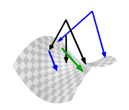
Figure 1: Visualization of the 5 projections from Example 3.2.

4 Further results

Recall that

$${C_{\alpha}}=\big{\{}{(x,y,\gamma)\in X\times X\times\mathbb{R}}~{}\big{|}~{}{\left\langle{x},{y}\right\rangle=\alpha\gamma}\big{\}},$$

and this is the representation more natural to use in Deep Learning (see [6]). Armed with Theorem 3.1, the projection onto ${C_{\alpha}}$ now readily obtained:

Theorem 4.1.

Let $(x_{0},y_{0},\gamma_{0})\in X\times X\times\mathbb{R}$. Then the following hold:

1. If $x_{0}\neq\pm y_{0}$, then

   $${\thinspace P\thinspace}_{\negthinspace\negthinspace{C_{\alpha}}}(x_{0},y_{0},\gamma_{0})=\bigg{\{}\Big{(}\dfrac{x_{0}-\lambda y_{0}}{1-\lambda^{2}},\dfrac{y_{0}-\lambda x_{0}}{1-\lambda^{2}},\gamma_{0}+\dfrac{\lambda\alpha}{\beta^{2}}\Big{)}\bigg{\}}$$

   for a unique $\lambda\in\left]-1,1\right[$ that solves the (essentially) quintic equation

   $$g(\lambda):=\frac{(\lambda^{2}+1)p-2\lambda q}{(1-\lambda^{2})^{2}}-\frac{2\lambda\alpha^{2}}{\beta^{2}}-2\alpha\gamma_{0}=0,$$

   where $p:=2\left\langle{x_{0}},{y_{0}}\right\rangle$ and $q:=\lVert x_{0}\rVert^{2}+\lVert y_{0}\rVert^{2}.$

2. If $y_{0}=-x_{0}\neq 0$, then we have the following:
   a) When $\alpha(\gamma_{0}-\frac{\alpha}{\beta^{2}})<-\frac{\|x_{0}\|^{2}}{4}$, then

   $${\thinspace P\thinspace}_{\negthinspace\negthinspace{C_{\alpha}}}(x_{0},-x_{0},\gamma_{0})=\bigg{\{}\Big{(}\dfrac{x_{0}}{1-\lambda},\dfrac{-x_{0}}{1-\lambda},\gamma_{0}+\dfrac{\lambda\alpha}{\beta^{2}}\Big{)}\bigg{\}}$$

   for a unique $\lambda\in\left]-1,1\right[$ that solves

   $$g_{1}(\lambda):=\frac{2\|x_{0}\|^{2}}{(1-\lambda)^{2}}+\frac{2\lambda\alpha^{2}}{\beta^{2}}+2\alpha\gamma_{0}=0.$$

   b) When $\alpha(\gamma_{0}-\frac{\alpha}{\beta^{2}})\geq-\frac{\|x_{0}\|^{2}}{4}$, then

   $${\thinspace P\thinspace}_{\negthinspace\negthinspace{C_{\alpha}}}(x_{0},-x_{0},\gamma_{0})=$$

   $$\quad\bigg{\{}{\Big{(}\dfrac{x_{0}}{2}+\dfrac{u}{\sqrt{2}},-\dfrac{x_{0}}{2}+\dfrac{u}{\sqrt{2}},\gamma_{0}-\dfrac{\alpha}{\beta^{2}}\Big{)}}~{}\bigg{|}~{}{\|u\|=\sqrt{2\alpha\Big{(}\gamma_{0}-\frac{\alpha}{\beta^{2}}\Big{)}+\frac{\|x_{0}\|^{2}}{2}},~{}u\in X}\bigg{\}}$$

   which is a singleton if and only if $\alpha(\gamma_{0}-\frac{\alpha}{\beta^{2}})=-\frac{\|x_{0}\|^{2}}{4}$.

3. If $y_{0}=x_{0}\neq 0$, then we have the following:
   a) When $\alpha(\gamma_{0}+\frac{\alpha}{\beta^{2}})>\frac{\|x_{0}\|^{2}}{4}$, then

   $${\thinspace P\thinspace}_{\negthinspace\negthinspace{C_{\alpha}}}(x_{0},x_{0},\gamma_{0})=\bigg{\{}\Big{(}\dfrac{x_{0}}{1+\lambda},\dfrac{x_{0}}{1+\lambda},\gamma_{0}+\frac{\lambda\alpha}{\beta^{2}}\Big{)}\bigg{\}}$$

   for a unique $\lambda\in\left]-1,1\right[$ that solves the (essentially) cubic equation

   $$g_{2}(\lambda):=\frac{2\|x_{0}\|^{2}}{(1+\lambda)^{2}}-\frac{2\lambda\alpha^{2}}{\beta^{2}}-2\alpha\gamma_{0}=0.$$

   b) When $\alpha(\gamma_{0}+\frac{\alpha}{\beta^{2}})\leq\frac{\|x_{0}\|^{2}}{4}$, then

   $${\thinspace P\thinspace}_{\negthinspace\negthinspace{C_{\alpha}}}(x_{0},x_{0},\gamma_{0})=$$

   $$\quad\bigg{\{}{\Big{(}\dfrac{x_{0}}{2}-\dfrac{v}{\sqrt{2}},\dfrac{x_{0}}{2}+\dfrac{v}{\sqrt{2}},\gamma_{0}+\dfrac{\alpha}{\beta^{2}}\Big{)}}~{}\bigg{|}~{}{\|v\|=\sqrt{-2\alpha\Big{(}\gamma_{0}+\frac{\alpha}{\beta^{2}}\Big{)}+\frac{\|x_{0}\|^{2}}{2}},~{}v\in X}\bigg{\}}$$

   which is a singleton if and only if $\alpha(\gamma_{0}+\frac{\alpha}{\beta^{2}})=\frac{\|x_{0}\|^{2}}{4}$.

4. If $x_{0}=y_{0}=0$, then we have the following:
   a) When $\alpha\gamma_{0}>\frac{\alpha^{2}}{\beta^{2}}$, then the projection is the non-singleton set

   $${\thinspace P\thinspace}_{\negthinspace\negthinspace{C_{\alpha}}}(0,0,\gamma_{0})=\bigg{\{}{\Big{(}\dfrac{u}{\sqrt{2}},\dfrac{u}{\sqrt{2}},\gamma_{0}-\frac{\alpha}{\beta^{2}}\Big{)}}~{}\bigg{|}~{}{\|u\|=\sqrt{2\alpha\Big{(}\gamma_{0}-\frac{\alpha}{\beta^{2}}\Big{)}},\,u\in X}\bigg{\}}.$$

   b) When $|\alpha\gamma_{0}|\leq\frac{\alpha^{2}}{\beta^{2}}$, then

   $${\thinspace P\thinspace}_{\negthinspace\negthinspace{C_{\alpha}}}(0,0,\gamma_{0})=\big{\{}(0,0,0)\big{\}}.$$

   c) When $\alpha\gamma_{0}<-\frac{\alpha^{2}}{\beta^{2}}$, then the projection is the non-singleton set

   $${\thinspace P\thinspace}_{\negthinspace\negthinspace{C_{\alpha}}}(0,0,\gamma_{0})=\bigg{\{}{\Big{(}-\dfrac{v}{\sqrt{2}},\dfrac{v}{\sqrt{2}},\gamma_{0}+\dfrac{\alpha}{\beta^{2}}\Big{)}}~{}\bigg{|}~{}{\|v\|=\sqrt{-2\alpha\Big{(}\gamma_{0}+\frac{\alpha}{\beta^{2}}\Big{)}},\,v\in X}\bigg{\}}.$$

Proof. With

$$A=\begin{bmatrix}\frac{1}{\sqrt{2}}\operatorname{Id}&-\frac{1}{\sqrt{2}}\operatorname{Id}&0\\ \frac{1}{\sqrt{2}}\operatorname{Id}&\frac{1}{\sqrt{2}}\operatorname{Id}&0\\ 0&0&1\end{bmatrix}$$

in mind, by Proposition 2.2(iii) we have

$${\thinspace P\thinspace}_{\negthinspace\negthinspace{C_{\alpha}}}[x_{0},y_{0},\gamma_{0}]^{\intercal} =A{\thinspace P\thinspace}_{\negthinspace\negthinspace{\widetilde{C}_{\alpha}}}A^{\intercal}[x_{0},y_{0},\gamma_{0}]^{\intercal}$$

$$=A{\thinspace P\thinspace}_{\negthinspace\negthinspace{\widetilde{C}_{\alpha}}}\Big{[}\frac{x_{0}+y_{0}}{\sqrt{2}},\frac{-x_{0}+y_{0}}{\sqrt{2}},\gamma_{0}\Big{]}^{\intercal}.$$

Hence (i)–(iv) follow by applying Theorem 3.1. $\hfill\quad\blacksquare$

Remark 4.2.

Theorem 4.1(i) was given in [6, Appendix B] without a rigorous mathematical justification.

It is interesting to ask what happens when $\alpha\rightarrow 0$.

Theorem 4.3.

Suppose that $X=\mathbb{R}^{n}$. Then ${\thinspace P\thinspace}_{\negthinspace\negthinspace{C_{\alpha}}}\stackrel{{\scriptstyle g}}{{\rightarrow}}{\thinspace P\thinspace}_{\negthinspace\negthinspace C\times\mathbb{R}}={\thinspace P\thinspace}_{\negthinspace\negthinspace C}\times\operatorname{Id}$ and ${\thinspace P\thinspace}_{\negthinspace\negthinspace{\widetilde{C}_{\alpha}}}\stackrel{{\scriptstyle g}}{{\rightarrow}}{\thinspace P\thinspace}_{\negthinspace\negthinspace\widetilde{C}\times\mathbb{R}}={\thinspace P\thinspace}_{\negthinspace\negthinspace\widetilde{C}}\times\operatorname{Id}$ when $\alpha\rightarrow 0$.

Proof. Apply Proposition 2.4 and 2.6. $\hfill\quad\blacksquare$

Remark 4.4.

The projection onto the cross $C$, ${\thinspace P\thinspace}_{\negthinspace\negthinspace C}$, has been given in [2].

References

- [1] J.-P. Aubin and H. Frankowska, Set-valued analysis, Springer Science & Business Media, 2009.
- [2] H. H. Bauschke, M. K. Lal, and X. Wang, The projection onto the cross, Set-Valued and Variational Analysis, 30 (2022), pp. 997–1009.
- [3] , Projections onto hyperbolas or bilinear constraint sets in hilbert spaces, Journal of Global Optimization, 86 (2023), pp. 25–36.
- [4] F. Bernard and L. Thibault, Prox-regular functions in hilbert spaces, Journal of Mathematical Analysis and Applications, 303 (2005), pp. 1–14.
- [5] D. P. Bertsekas, Nonlinear programming, Journal of the Operational Research Society, 48 (1997), pp. 334–334.
- [6] V. Elser, Learning without loss, Fixed Point Theory and Algorithms for Sciences and Engineering, 2021 (2021), p. 12.
- [7] E. Kreyszig, Introductory functional analysis with applications, vol. 17, John Wiley & Sons, 1991.
- [8] B. Odehnal, H. Stachel, and G. Glaeser, The universe of quadrics, Springer Nature, 2020.
- [9] R. T. Rockafellar and R. J. B. Wets, Variational Analysis, vol. 317, Springer, Berlin.