Detecting bifurcations in dynamical systems with CROCKER plots

Abstract

Existing tools for bifurcation detection from signals of dynamical systems typically are either limited to a special class of systems, or they require carefully chosen input parameters, and significant expertise to interpret the results. Therefore, we describe an alternative method based on persistent homology—a tool from Topological Data Analysis (TDA)—that utilizes Betti numbers and CROCKER plots. Betti numbers are topological invariants of topological spaces, while the CROCKER plot is a coarsened but easy to visualize data representation of a one-parameter varying family of persistence barcodes. The specific bifurcations we investigate are transitions from periodic to chaotic behavior or vice versa in a one-parameter black collection of differential equations. We validate our methods using numerical experiments on ten dynamical systems and contrast the results with existing tools that use the maximum Lyapunov exponent. We further prove the relationship between the Wasserstein distance to the empty diagram and the norm of the Betti vector, which shows that an even more simplified version of the information has the potential to provide insight into the bifurcation parameter. The results show that our approach reveals more information about the shape of the periodic attractor than standard tools, and it has more favorable computational time in comparison to the Rösenstein algorithm black for computing the maximum Lyapunov exponent.

Qualitative changes in the system response such as transitions from regular to chaotic behavior are referred to as bifurcations. When the system is modeled by differential equations with a large number of degrees of freedom, or if all that is available is a time series from a system observable, detecting these bifurcations becomes challenging. Therefore, we focus on a data-driven approach for bifurcation detection where we measure properties of embedded time series to determine if and when the behavior of the system has changed. The tools used come from topological data analysis (TDA), where shape is quantified using tools from algebraic topology. The contribution of this paper is to show how the CROCKER plot Topaz, Ziegelmeier, and Halverson (2015), a visual tool for analysis of changing shape, can be used for the purpose of analyzing and detecting bifurcations. Further, compressed versions of this information by taking the norm over columns of the resulting matrix can also be associated to changes in the system. The analysis is performed by testing the ideas empirically on ten dynamical systems and providing comparisons to standard bifurcation analysis tools.

I Introduction

Systems expressing chaotic behavior can be found in a variety of domains, ranging from mathematics to biology, economics to electrical circuits, and engineering to social sciences. When considering chaotic systems in terms of engineering applications, the major issue is determining how to control complexity and unpredictability. As the number of features in established systems grows, the system becomes more complicated, making modeling the system more difficult. Further, since the definition of bifurcation is quite qualitative, we are left to either qualitative measurements, or turn to other quantitative measures which tend to be computationally expensive options for analysis. In this paper, we propose a method for investigating bifurcations in dynamical systems using a tool from topological data analysis (TDA) called the CROCKER plot Topaz, Ziegelmeier, and Halverson (2015).

There is a growing literature dedicated to connecting dynamical systems analysis with TDA to create new data-driven analysis tools, a field collectively known as Topological Signal Processing (TSP) Robinson (2014). The original seeds of TDA as a field were planted through connections with dynamical systems Robins, Meiss, and Bradley (2000); Kaczynski, Mischaikow, and Mrozek (2004), so it is no surprise that these ideas can be quite useful for time series analysis. Much of the recent work utilizes persistent homology, colloquially known as persistence, which encodes the shape and structure of given input data by providing measurements of features such as clusters and holes. The standard and highly utilized pipeline for time series data Khasawneh and Munch (2017); Garland, Bradley, and Meiss (6 11); Mittal and Gupta (2017); Dee Algar, Corrêa, and Walker (2021); Güzel and Kaygun (2022); Karan and Kaygun (2021); Maletić, Zhao, and Rajković (2016); Marchese and Maroulas (2017); Kim, Kim, and Rinaldo (2018); Seversky, Davis, and Berger (2016); Venkataraman, Ramamurthy, and Turaga (2016); Perea and Harer (2015); Perea (2019); Berwald, Gidea, and Vejdemo-Johansson (2014); Tan et al. (2021) is as follows. Take a time series of interest, generate a point cloud from it using a delay coordinate embedding, create a filtration of the complete simplicial complex using the Rips construct, and compute the persistent homology of the result. From here, the analysis tools depend on the types of input data and conclusions desired, but nearly all involve some form of featurization of the resulting persistence diagrams. This process, which returns some form a vector representing the persistence diagram, is required as the unusual geometry of the space of diagrams Bubenik and Wagner (2020) results in limitations when passing the information as inputs to machine learning algorithms. This pipeline has found a great deal of success in both theory and applications, including machining Yesilli et al. (2019); Khasawneh and Munch (2016, 2018), finance Gidea (2017); Gidea and Katz (2018); Gidea et al. (2020); Rivera-Castro, Pilyugina, and Burnaev (2019); Majumdar and Laha (2020), and biomedicine Ignacio et al. (2019); Stolz, Harrington, and Porter (2017); Majumder et al. (2020); Chung et al. (2021); Emrani, Gentimis, and Krim (2014). More recently, work has begun to modify aspects of this pipeline Tymochko, Munch, and Khasawneh (2020); Myers, Munch, and Khasawneh (2019); Myers, Khasawneh, and Munch (2022); Bauer et al. (2020); Tempelman and Khasawneh (2020); Khasawneh and Munch (2018) or to accept different forms of data input than simple time series Myers, Khasawneh, and Munch (2 05); Tralie (2016); Tymochko et al. (2020); Tralie and Perea (2018); Levanger et al. (2019); Wu and Hargreaves (2021).

In this paper, we focus on the case of time series data associated to a bifurcation parameter. That is, a parameter which can be changed in the system resulting in different types of output behavior. With a collection of time series, each associated to this parameter value, we can employ tools from TDA which are built to handle a 1-parameter family of persistence diagrams. While this collection of methods includes multiparameter persistence Kim and Mémoli (2021), and vineyards Cohen-Steiner, Edelsbrunner, and Morozov (2006), we will focus on the CROCKER plot Topaz, Ziegelmeier, and Halverson (2015) due to its simple visualization. The idea is that for each value of the bifurcation parameter, there is a persistence diagram computed from the time series via the normal pipeline, but this can instead be encoded via its simpler Betti curve. These Betti curves, which are vectorized into columns, can be collected into a matrix to easily visualize changes in the persistence diagram structure, which can then be interpreted against the original bifurcation parameter for analysis of the system.

The result, called a CROCKER plot, was originally developed in the context of dynamic metric spaces Topaz, Ziegelmeier, and Halverson (2015); Ulmer, Ziegelmeier, and Topaz (2019); Bhaskar et al. (2019); Xian et al. (2022). There, the additional restrictions means that the time-varying point clouds under study have labels on vertices from one parameter value to the next, allowing for more available theoretical results on continuity. However, the visualization tool itself needs no such assumption, as we have no tracking information on our point clouds from one step to the next.

In this paper, we show that the CROCKER plot can be used as both a qualitative and quantitative tool for understanding bifurcations in dynamical systems. We will also begin to look at an even more simplified version of the information, namely the $L_{1}$ norm of the Betti curves. As we show that this construction is closely related to the 1-Wasserstein distance commonly used for persistence diagrams and make connections between this and the maximum Lyapunov exponent, a commonly used measure for chaos. This paper is the full version of our short conference paper Güzel, Munch, and Khasawneh (2022).

Outline.

We organize this paper as follows. In Sec. II we give the necessary background on dynamical systems, persistent homology, and CROCKER plots. In Sec. III, we give specifics of the method, and show the results with full details on the Lorenz and Rössler systems, with further results shown for a longer list of example dynamical systems. Finally, we discuss conclusions, limitations, and future work in Sec. IV.

II Background

In this section, we give the necessary background for the CROCKER based analysis of dynamical systems. In particular, we discuss needed dynamical systems background in Sec. II.1; and the topological tools we use in Sec. II.2.

II.1 Dynamical systems

Throughout this work, we assume that we have access to sampled realizations of a dynamical system $X=[x_{1},\cdots,x_{N}]$ where $x_{i}\in\mathbb{R}^{n}$ and have the goal of analyzing changes in the behavior in a data-driven manner. In this paper, we use two main tools from the dynamics literature for analyzing the dynamics of a non-linear system. Namely, we first use the bifurcation diagram which is a qualitative measure and Lyapunov exponent which is a quantitative measure. As these tools are standard in nonlinear time series analysis, we direct the interested reader to textsKantz and Schreiber (2003); Hirsch, Smale, and Devaney (2013); Baker and Gollub (1996); Sayama (2015) for further details.

II.1.1 Bifurcation Diagrams

A bifurcation in a dynamical system is characterized by tiny changes in parameter values causing qualitative changes in the behavior. These result in qualitative changes in the system’s equilibrium point or the unstable state of stable equilibrium points. Hence, detecting them is critical since they can indicate when a system is transitioning from normal operation to imminent breakdown. Bifurcations can occur in both continuous and discrete time systems, and we call the system parameter that produces the bifurcation event the bifurcation parameter. One visual tool for finding bifurcations is the bifurcation diagram, which shows local extrema of a given system over a varying control parameter while keeping other parameters fixed.

An example of this can be seen in Fig. 1(a) for the commonly studied Lorenz system Lorenz (1963). This system is given by the equations

$$\dot{x}=\sigma(y-x),\quad\dot{y}=x(\rho-z)-y,\quad\dot{z}=xy-\beta z,$$

where the constants $\sigma,\rho,\beta$ are system parameters, $x$ is proportional to the rate of convection, and $y$ and $z$ are the horizontal and vertical temperature variation, respectively. In the example of Fig. 1(a), we show the bifurcation diagram with respect to varying the parameter $\rho$ with 600 equally spaced values between 90 and 105; and with the $\sigma$ and $\beta$ parameters remaining constant. The attractor for four marked values of $\rho$ can be seen above the bifurcation diagram in Fig. 1. black The Lorenz system was simulated using DynamicalSystems.jl  Datseris (2018) package in julia Bezanson et al. (2017) with default function parameters. As we see from Fig. 1, there are two obvious periodic regions around $\rho=92.1$ and $\rho=100.1$. However, a limitation of bifurcation diagrams is their inherently qualitative nature, meaning further tools are required for understanding bifurcations.

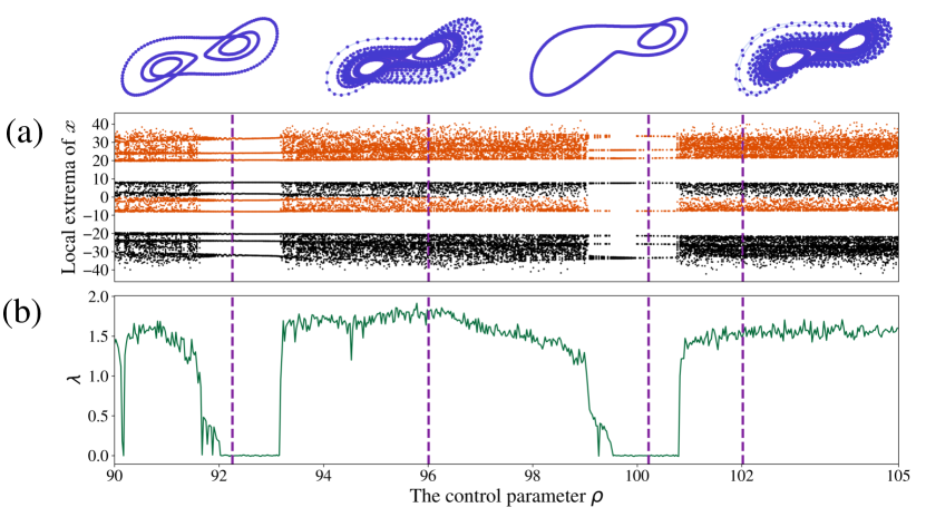
Figure 1: The bifurcation diagram (a) and the maximum Lyapunov exponent (b) for the Lorenz system with varying 600 $\rho$ parameters between 90 and 105 and $\sigma=10,\>\beta=8/3$. On the bifurcation diagram, the black orange scatter plot represents local maxima while black black represents local minima of the variable $x$.

II.1.2 The maximum Lyapunov exponents

The second tool we use to investigate the behavior of a system, in this case, a quantitative measure, is called the maximum Lyapunov exponent. It can be described as the mean rate of exponential divergence or convergence of two neighboring beginning points in the phase space of a dynamical system. Specifically, the quantity is defined as follows.

Definition II.1.

Given a dynamical system $\dot{Z}=F(Z)$ with $n-$dimensional phase space, we consider two neighboring trajectories $Z(t)$ and $Z(t)+\delta(t)$, where $\delta(t)$ is a vector with infinitesimal initial length. The maximum Lyapunov exponent of the system is a number $\lambda$, if it exists, such that $||\delta(t)||\thickapprox||\delta(0)||e^{\lambda t}$. Specifically,

$$\lambda=\lim_{t\to\infty}\frac{1}{t}\log\frac{\|\delta(t)\|}{\|\delta(0)\|},$$

where $\|\cdot\|$ is the Euclidean norm. Moreover, the system is called chaotic if $\lambda>0$, periodic if $\lambda=0$ and stable if $\lambda<0$.

black We use the maximum Lyapunov exponent as our ground truth measurement for whether a dynamical system is chaotic, periodic, or stable at a given parameter value, and make use of two different algorithms for its computation. First, we use the Benettin algorithm Benettin et al. (1980) to compute the maximum Lyapunov exponent in the case that we are assumed to have a model of the dynamical system. In particular, analytical calculations (when possible) are computationally expensive since they require the Jacobian matrix.

However, as is often the case in practice, when the model of the dynamical system is not available, we turn to numerical approximations. In our experiments, the maximum Lyapunov exponent is numerically computed using Rösenstein’s algorithm Rösenstein, Collins, and De Luca (1993). In this algorithm, the maximum Lyapunov exponent is calculated using the slopes of the average divergence curves that result from linear fits of a scaling region. However, human input is required for the results of this procedure to be a reliable approximation for the true Lyapunov exponent. That being said, this algorithm is still commonly used in practice and thus it is useful to explore the relationships between the Rösenstein results and the TDA methods introduced here. The experiments described in Sec. III involve far too many time series to be able to perform detailed human checking, so we only use these results as an approximation and show further information on the challenges and quality of approximation for our experiments in Appx. A.

black Returning to the example of Fig. 1(b), we see the maximum Lyapunov exponent, labeled $\lambda$, on the bottom of the figure. We calculated this maximum Lyapunov exponent from the model by using Benettin algorithm implementation in DynamicalSystems.jl. Note that there are still errors in the Benettin algorithm, since, for example, in the regions around 92.1 and 100.1, $\lambda$ approaches 0, but due to approximation errors does not stay at exactly 0. Further, we can see that regions around these parameter values sometimes have non-zero Lyapunov exponent despite having visually periodic behavior in the bifurcation diagram. We will further investigate this situation in the experiment section, Sec. III.

II.2 Topological Data Analysis

A modern tool for measuring the shape of data, particularly point cloud data of the form we have sampled for a given dynamical system $X=[x_{1},\cdots,x_{N}]$, is that of persistent homology and related ideas. This construction comes from the field of topological data analysis Dey and Wang (2022); Oudot (2017); Munch (2017), and has many variants, including Betti curves, persistence diagrams, and persistence barcodes. In this paper, we will focus on the CROCKER plot Topaz, Ziegelmeier, and Halverson (2015), which is a relative of persistence in the case of a parameter stream of data, and provide the background needed for its definition.

II.2.1 Persistent homology

The idea behind persistent homology is that we can encode information about a fixed shape using homology Hatcher (2002); Munkres (1984), and extend this idea to develop a filtration of shapes where we can measure the changing homology. In this section, we give a view of the basics but direct the interested reader to relevant texts Dey and Wang (2022); Oudot (2017) for further specifics.

The data we study in this work are point clouds, i.e. a finite discrete sets of points $X\subset\mathbb{R}^{N}$. We can develop a filtration of simplicial complexes based on this point cloud using the Vietoris-Rips complex, defined as follows.

Definition II.2.

Given a point cloud $X$, the Vietoris-Rips complex is defined to be the simplicial complex whose simplices are built on vertices that are at most $\varepsilon$ apart,

$$R_{\varepsilon}(X)=\{\sigma\subset X\mid d(x,y)\leq\varepsilon,\text{ for all }x,y\in\sigma\}.$$

When $X$ is clear from context, we denote the complex simply by $R_{\varepsilon}$.

For a fixed $\varepsilon$, we get a fixed simplicial complex $R_{\varepsilon}(X)$. These complexes have the additional property that for $\varepsilon\leq\varepsilon^{\prime}$, $R_{\varepsilon}(X)\subseteq R_{\varepsilon^{\prime}}(X)$. The resulting collection of Vietoris-Rips complexes for a sequence of proximity parameters, $\varepsilon_{0}\leq\varepsilon_{1}\leq\cdots\leq\varepsilon_{s}$, is the filtration

$$R_{\varepsilon_{0}}\subseteq R_{\varepsilon_{1}}\subseteq\cdots\subseteq R_{\varepsilon_{s}}.$$

An example of this construction can be seen in Fig. 2(a-d).

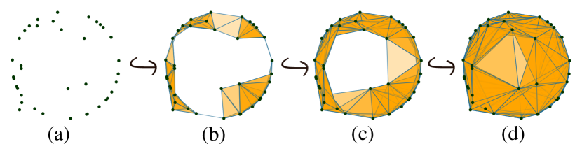
Figure 2: The Vietoris-Rips complex for four choices of an increasing proximity parameter $\varepsilon$. The 1-dimensional Betti numbers, which count the number of loops in each complex, are 0, 1, 1 and 0 in order from left (a) to right (d).

To measure the changing shape, we turn to homology. For a given simplicial complex $K$, the $k$-dimensional homology $H_{k}(K)$ is a vector space representing $k$-dimensional structure in the complex. The lowest dimensions come with the most intuition; namely that 0-dimensional homology measures connected components, 1-dimensional homology measures loops, and 2-dimensional homology measures voids. We direct the interested reader to classical textsHatcher (2002); Munkres (1984) for the full specifics on homology. For our purposes, the important information is that the basis of the vector space $H_{k}(K)$ has one element per $k$-dimensional structure. The dimension of $H_{k}(K)$ is called the $k^{\text{th}}$ Betti number, and will play an important role in the next section. So, in the case of 1-dimensional homology in the example of Fig. 2, the $1^{\text{st}}$ Betti numbers for each simplicial complex shown are 0, 1, 1, and 0, respectively as only the second and third complexes, (b) and (c) have a loop.

Of course, in the example of Fig. 2, we can see that for certain choices of $\varepsilon$ proximity parameters, the structure of the Vietoris-Rips complex $R_{\varepsilon}(X)$ is a good approximation for the structure seen in the point cloud; namely that the points appear to be sampled from a circle. However a priori, we have no working knowledge to determine the right choice of $\varepsilon$ in advance, especially when we happen to not be working with a point cloud in low dimensions like $n=2$. To this end, we turn to persistent homology, which encodes information about all values of $\varepsilon$ at once, allowing us to measure the durability of topological features over the changing parameter.

The additional tool we use is that the vector spaces $H_{k}(R_{\varepsilon}(X))$ also come with linear maps induced by the inclusions $R_{\varepsilon}(X)\hookrightarrow R_{\varepsilon^{\prime}}(X)$. While we again leave specifics to classical texts Hatcher (2002); Munkres (1984), the result is a collection of vector spaces and maps

$$H_{k}(R_{\varepsilon_{0}})\rightarrow H_{k}(R_{\varepsilon_{1}})\rightarrow\cdots\rightarrow H_{k}(R_{\varepsilon_{s}})$$

called a persistence module.

Further results in algebra mean that the persistence module can be decomposed into interval modules, which effectively give information about when features measured by homology appear and disappear over the module. Details can be found in Oudot (2017). black This data can be uniquely represented through a collection of pairs $(\varepsilon_{b},\varepsilon_{d})$ in a decomposition of the module, where each pair represents the parameter values for which a homological feature appeared at time $b$ and disappeared at time $d$. To visualize this information, we turn to the persistence diagram, where an example can be seen in Fig. 3.

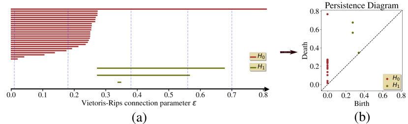
Figure 3: The persistence barcode with Vietoris-Rips complex for chosen epsilon parameters (a) and corresponding persistence diagram (b). The Vietoris-Rips filtration parameters $[0.01,0.18,0.38,0.56,0.7]$ and 1-dimensional Betti numbers corresponding to given filtration parameter $\varepsilon$ is $[0,0,2,2,0]$ .

Definition II.3.

A persistence diagram is a finite collection of off-diagonal points

$$D=\{(b,d)\in\mathbb{R}^{2}\mid b<d\}$$

where $b$ and $d$ are the birth and death time of a feature in the persistence module. We call with $d-b$ the lifetime of the feature.

The empty diagram is the diagram with no off-diagonal points, $D_{\emptyset}=\{\}.$

A persistence barcode encodes the same information as the persistence diagram, but instead, is a collection of horizontal line segments as in Fig. 3. We place the homology generators on the vertical axis (where order does not matter) whereas the horizontal axis represents the life span of each homology class in terms of the parameter $\varepsilon$. When we draw the vertical line at a particular $\varepsilon_{i}$, the number of intersecting line segments in barcodes is the dimension of the corresponding homology group, i.e. the Betti number for that parameter $\varepsilon_{i}$. In Fig. 3, one can see barcodes together with the Vietoris-Rips complex corresponding to several choices of $\varepsilon$.

One of the reasons these persistence diagrams are so useful is the availability of metrics for their comparison. We focus here on the family of Wasserstein distances for persistence diagram, which effectively measure how easily the points in two diagrams can be matched up. To handle diagrams of different sizes, we allow for unmatched points in the two diagrams.

Definition II.4.

A partial matching between two diagrams $D_{1}$ and $D_{2}$ is a bijection $\mathbb{M}:S_{1}\rightarrow S_{2}$ where $S_{1}\subset D_{1}$ and $S_{2}\subset D_{2}$. Two points $\alpha_{1}\in D_{1}$ and $\alpha_{2}\in D_{2}$ are called matched when $\alpha_{2}=\mathbb{M}(\alpha_{1})$ while an element $\alpha_{1}\in(D_{1}\backslash S_{1})\cup(D_{2}\backslash S_{2})=:U_{\mathbb{M}}$ is called unmatched. The Wasserstein distance between a pair of diagrams $D_{1}$ and $D_{2}$ is defined as

$$W_{q}(D_{1},D_{2})=\inf_{\mathbb{M}}\left(\sum_{(\alpha_{1},\alpha_{2})\in\mathbb{M}}\|\alpha_{1}-\alpha_{2}\|_{\infty}^{q}+\frac{1}{2^{q}}\sum_{\alpha\in U_{\mathbb{M}}}|\alpha_{d}-\alpha_{b}|^{q}\right)^{1/q},$$

where the infimum is taken over all possible partial matches $\mathbb{M}\subset D_{1}\times D_{2}$.

See the example of Fig. 4, where two diagrams are overlaid. In Fig. 4(b), a poor choice of matching results in a high matching cost, while the matching shown at right Fig. 4(c) achieves the infimum and thus the Wasserstein distance between the diagrams.

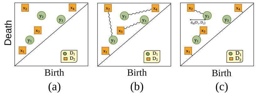
Figure 4: Consider several choices of matchings used in Defn.  II.4 for two diagrams $D_{1}$ and $D_{2}$ shown overlaid in (a). One option for a matching is shown in (b), but the best matching based on the cost is given in (c).

II.2.2 Betti curves and Betti vectors

Despite losing some information in the process, another useful representation of the changing shape is to simply watch the changing rank of the homology rather than tracking the full homology along the filtration. Recall that the $k^{\text{th}}$ Betti number is the dimension of the $k^{\text{th}}$ homology group, denoted $\beta_{k}(K)=\dim(H_{k}(K))$. Then in our setting, the Betti curve is the function encoding the Betti number for each choice of $\varepsilon$ proximity parameter in the Vietoris-Rips complex.

Definition II.5.

Fix a point cloud $X$ and denote the Vietoris-Rips complex at proximity parameter $\varepsilon$ by $R_{\varepsilon}(X)$. Then the Betti curve is a function

$$\begin{matrix}B_{X}:&\mathbb{R}&\longrightarrow&\mathbb{N}\\ &\varepsilon&\longmapsto&\beta_{k}(R_{\varepsilon}(X)).\end{matrix}$$

We further have a discretized version of the Betti curve, called the Betti vector, which encodes the information from the Betti curve at a fixed sequence of $\varepsilon$ values.

Definition II.6.

Let $P=\{\varepsilon_{0},\varepsilon_{1},\dots,\varepsilon_{s}\}$ be a partition of the interval $(\varepsilon_{0}=0,\varepsilon_{s})$. The $k$-dimensional Betti vector is defined as the ordered sequence of the $k$-dimensional Betti numbers, that is

$$Bv_{k}(X;P)=(\beta_{k}(R_{\varepsilon_{0}}),\beta_{k}(R_{\varepsilon_{1}}),\dots,\beta_{k}(R_{\varepsilon_{s}})).$$

One particularly useful property of the Betti curve viewpoint over the persistence diagram is that we have access to a norm. In particular, for any $p\in(0,\infty]$, the $L_{p}$ norm of a real-valued function $f$ is

$$||f||_{p}=\left(\int|f(x)|^{p}dx\right)^{1/p}.$$

Even though it is known that the Betti curves are unstable Johnson and Jung (2021); Chung and Lawson (2022), there is a close relationship between the norm of the Betti curve and the Wasserstein distance between a given diagram and the empty diagram. Specifically, this is encompassed in the following proposition which is proved in Appendix B.

Proposition II.1.

Let $D$ be a persistence diagram with maximum death time $d_{max}$, and $\mathbb{I}=(0,d_{max})\subset\mathbb{R}$. Then, the link between Betti curves and Wasserstein distance is given by

$$\int_{\mathbb{I}}B_{D}(s)\ ds=2\cdot W_{1}(D,D_{\emptyset}).$$

black This proposition implies that even if they are not stable (which should be thought of in analogue to Lipschitz functions), the Betti curves are at least continuous with respect to variations in the input data. This result comes from combining the above proposition with the the stability theorem for Wasserstein distance Cohen-Steiner et al. (2010); Skraba and Turner (2020).

II.2.3 CROCKER plots

The data we analyze here is not a single point cloud, but instead one point cloud realization $\{X_{\eta}\}_{\eta\in\mathcal{A}}$ per parameter value of the parameter space of interest $\mathcal{A}=\{\eta_{0},\cdots,\eta_{m}\}$ in the dynamical system. Thus in the framework above, we get one persistence diagram per parameter value $\{D_{\eta}\}_{\eta\in\mathcal{A}}$. There have been several methods proposed for accommodating analysis of data of this form. These include multiparameter persistence Carlsson and Zomorodian (2009), and vineyards Cohen-Steiner, Edelsbrunner, and Morozov (2006). However, mathematical limitations and obfuscating interpretations make these difficult to work with. For this reason, we look at one of the most accessible representations of this data, the Contour Realization Of Computed $k$-dimensional hole Evolution in the Vietoris-Rips complexTopaz, Ziegelmeier, and Halverson (2015), also known as a CROCKER plot.

While much of the original work Topaz, Ziegelmeier, and Halverson (2015); Ulmer, Ziegelmeier, and Topaz (2019) was focused on the special case of time-varying point clouds (where the $i^{\text{th}}$ point in the cloud black $X_{\eta}$ is related to the $i^{\text{th}}$ point in cloud $X_{\eta+\varepsilon}$, e.g. Kim and Mémoli (2021)), there is no need for such a requirement. Indeed all we need is a sequence of Betti vectors, as in Defn. II.6, over a changing parameter.

Definition II.7.

Fix a partition of proximity parameters $P=\{0,\varepsilon_{1},\cdots,\varepsilon_{s}\}$ and a partition of the parameter space of interest $\mathcal{A}=\{\eta_{0},\cdots,\eta_{m}\}$. Denote the collection of point clouds by $\mathcal{X}=\{X_{\eta_{i}}\}_{i=0}^{m}$. Then the $k^{\text{th}}$ CROCKER plot is the discrete function

$$CP(\mathcal{X})[\eta_{i},\varepsilon_{j}]=\beta_{k}(R_{\varepsilon_{j}}(X_{\eta_{i}})).$$

Note that viewed as a matrix, the CROCKER plot is the Betti vectors for each $\alpha$ value stacked horizontally,

$$CP(\mathcal{\mathcal{X}})=\begin{pmatrix}|&|&&|\\ Bv(X_{\eta_{0}};P)&Bv(X_{\eta_{1}};P)&\cdots&Bv(X_{\eta_{m}};P)\\ |&|&&|\end{pmatrix}.$$

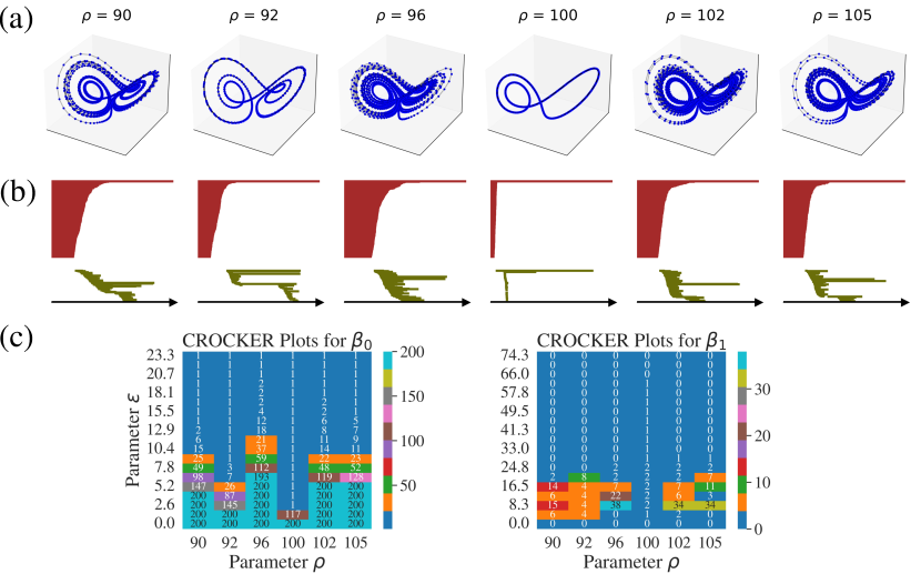
Figure 5: An example showing the CROCKER plots (bottom row (c); dimensions 0 and 1) for a coarse partitioning of the $\rho$ parameter for the Lorenz system in the first row (a). The corresponding persistence barcodes are shown in the middle row (b).

Consider the example of Fig. 5, where we have six realizations of the Lorenz system for choices of the different $\rho$ in Fig. 5(a). The barcode for each is shown in the next row Fig. 5(b). The $0$ and $1$-dimensional CROCKER plots are shown at the bottom Fig. 5(c) as the heat maps. Each of the 6 columns is the Betti vector for the corresponding realization. The high values of Betti numbers for the low $\varepsilon$ values come from the many short bars present in the noisy systems. Overarching circular structure, which shows up as long bars in the barcode, appear as positive values that stretch up into the higher $\varepsilon$ values.

The goal of this paper is to use these CROCKER plots to measure the changing topological behaviour of dynamics of nonlinear systems while varying both a system parameter and the Rips proximity parameter. Unlike tools used in classic bifurcation analysis, the only needed input is the reconstructed point cloud of the attractor. In the following section, we will show examples for how this plot can be used to find bifurcations in the behavior of dynamical systems.

III Experiments and Results

After giving specifics of the choices made in the method, in this section we show the pipeline as applied to two nonlinear dynamical systems: the Rössler system and Lorenz system. We then give similar results for a longer list of systems, with further details of each in Appendix D.

III.1 Specifics for the method

Our experiments will test this pipeline for the CROCKER plots as an analysis tool for bifurcation in dynamical systems. While the method itself can be seen in the example Fig. 5, we provide additional specifics and choices in this section.

black The dynamical systems were simulated using DynamicalSystems.jl  Datseris (2018) package in julia Bezanson et al. (2017). We also calculate the maximum Lyapunov exponents based on Benettin algorithm in same library. We then fetch the states of dynamical system as a point cloud for the python programming language to continue on CROCKER tasks. Due to the high density of points in the resulting point clouds and computational expense of persistence diagrams, we subsampled each realization $X_{\eta}$ using a greedy sub-sampling algorithm Cavanna, Jahanseir, and Sheehy (2015) resulting in 500 points per point cloud. We then compute the $0$- and $1$-dimensional persistence diagrams $D_{\eta}$ using ripser Tralie, Saul, and Bar-On (2018).

We compute all simulations prior to choosing the partition $P$ so as to ensure that we cover a range that includes all points in the persistence diagrams. Specifically, if $M$ is the maximum death time of any point in all the $k$-dimensional persistence diagrams (excluding the $\infty$-point present in all $0$-dimensional diagrams), we evenly split the interval $[0,M]$ into 100 pieces. Thus $P=\{0,\tfrac{1}{100}\cdot M,\tfrac{2}{100}\cdot M,\cdots,M\}$. With this fixed choice of partition, we can then use the persistence diagrams to get the Betti vectors using the equation $\beta_{k}(R_{\varepsilon}(X_{\eta}))=\#\{(b,d)\in D_{\eta}\mid b\leq\varepsilon<d\}$. Note that in theory, one could speed up computation by computing the Betti vectors for a given partition directly without computing the full persistence diagrams first; however all software we are aware of returns the Betti vectors by computing the full diagram first.

III.2 Rössler System

The Rössler system is given by the equations

$$\dot{x}=-y-z,\quad\dot{y}=x+ay,\quad\dot{z}=b+z(x-c).$$

For this study, we fixed parameters $b=2$ and $c=4$. We then vary the control parameter $a$ for 600 equally spaced values between 0.37 and 0.43. We used a sampling rate of 15 Hz for 1000 seconds and the initial conditions black $[x,y,z]=[-0.4,0.6,1]$. After solving the system, we retain the last 170 seconds to avoid transients.

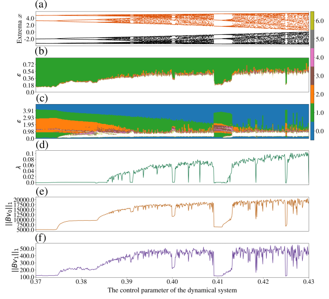
Figure 6: The bifurcation diagram (a) and Lyapunov exponent (d) are shown for the Rössler system varying the control parameter $a$. The 0- and 1-CROCKER plots (b and c respectively) and $L_{1}$ norm of each Betti vector (e and f) are also shown.

In Fig. 6(a), we show the bifurcation diagram for the Rössler system varying parameter $a$ with 600 equally-spaced values between 0.37 and 0.43 with the other parameters fixed. The local maxima and minima values of the system variable $x$ are colored black orange and black black, respectively. Below this are the CROCKER plots for homology dimensions 0 (Fig. 6(b)) and 1 (Fig. 6(c)). The value of the Betti number is shown by color; white regions are values for which black $\beta_{k}>6$. In these cases, those regions are largely viewed as noise. For instance, the large white region in the 0-CROCKER is caused by small values of $\varepsilon$ resulting in many individual connected components in $R_{\varepsilon}(X)$. Indeed, for small enough $\varepsilon$, this is one component per point in the cloud. The timing for these components merging up is a result of density of the sampling of the realization of the dynamical system. As such, the white region in the 0-CROCKER plot here is largely a measure of our subsampling required to compute persistence on a smaller point cloud. Periodic regions include multiple runs along the attractor, thus increasing the density of coverage and resulting in earlier mergings in the 0-dimensional diagram.

Thanks to these visualization tools, we can qualitatively compare the CROCKER plots with the bifurcation diagram. Note that most markedly around the bifurcation that occurs around $a=0.41$, there is a clear shift in the CROCKER plots as well as in the bifurcation diagram. This occurs both in the 0- and 1-dimensional diagrams. In the 0-dimensional CROCKER plot, there is a drop in the maximum $\varepsilon$ (vertical axis) at which the Betti curve becomes a constant 1. The 1-dimensional CROCKER plot has a marked shift in the maximum $\varepsilon$ value for which the Betti curve is positive, meaning this persistence diagram has a long lived bar. Further, the thick brown region ($\beta_{1}=3$) implies there are likely two additional long lived bars in the persistence diagrams in this area.

Moreover, when we vertically look at 1-dimensional CROCKER, the system has two prominent circular shapes in the system parameters interval between 0.37 and 0.39. For instance, one of them has a lifetime of approximately 4 ($\varepsilon_{b}\approx 0.2,\>\varepsilon_{d}\approx 4.02$) while the other one has a lifetime of 2 ($\varepsilon_{b}\approx 0.9,\>\varepsilon_{d}\approx 2.9$) at the system parameter 0.37. On the other hand, when we horizontally drive the system parameter to the right sides between the parameters 0.39 and 0.42, these 2 loops will change into a circular shape since one of them disappeared.

There is an even further simplified version of viewing the data, namely the $L_{1}$ norm of the Betti vector. For partition $P=\{\varepsilon_{0},\cdots,\varepsilon_{s}\}$, this is given as

$$\|Bv_{k}(X;P)\|_{1}=\sum_{\forall i}\beta_{k}(R_{\varepsilon_{i}}).$$ (1)

These graphs are shown in parts (e) and (f) of Fig. 6. Again, we can see qualitative similarities, in particular when comparing the graphs of the $L_{1}$ norms with the maximum Lyapunov exponent graph $\lambda$ black obtained from Benettin algorithm.

For a more quantitative test, we compute the Pearson correlation coefficient between the black maximum Lyapunov exponent and the $L_{1}$ norms for 0- and 1-dimensional information. Full details of this computation are given in Appendix C, but the idea is that values close to 1 imply a strong positive linear correlation. For our cases, the computed Pearson coefficient values were black 0.88 and 0.85, respectively. This means that there is a strongly positive correlation between them.

III.3 Lorenz System

We run the same test on Lorenz system which consists of three ordinary differential equations,

$$\dot{x}=\sigma(y-x),\quad\dot{y}=x(\rho-z)-y,\quad\dot{z}=xy-\beta z.$$

Here the parameters $\sigma=10$ and $\beta=8/3$ are fixed, while the control parameter $\rho$ is varied across 600 equally spaced values in the interval $[90,105]$. The solutions are simulated using a sampling rate of 100 Hz for 100 seconds with the initial conditions $[x,y,z]=[10^{-10},0,1]$. After solving the system, we take the last 20 seconds to avoid transients.

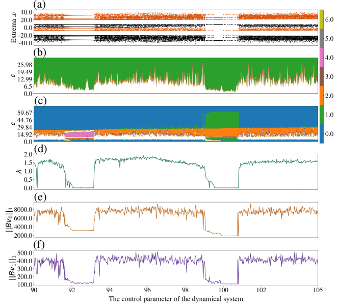
Figure 7: The bifurcation diagram (a), the 0- and 1- dimensional CROCKER plots (b and c, respectively), the maximum Lyapunov exponents (d) and for each CROCKER plots , the $L_{1}$ norm of each Betti vector (e and f) corresponding to varying the control parameter $\rho$ for the Lorenz system.

In Fig. 7, as in the Rössler system, Lorenz’s CROCKER and $L_{1}$ norms exhibit similar characteristics to the bifurcation diagram and the maximum Lyapunov exponent. We also note that there is a clear relationship between the maximum Lyapunov exponent and the $L_{1}$ norm of the CROCKER vectors as seen on the Fig. 7(d-f). The computed Pearson coefficient values between the maximum Lyapunov exponent, and the $L_{1}$ norms for 0- and 1-dimensional Betti vectors were 0.93 in both cases.

However, when we examine two different system parameters in the same system, some differences emerge in the case of 1-dimensional CROCKER. In particular as shown in Fig. 8, consider the parameters $\rho$ around 92.5 and 100. While in the 0-dimensional CROCKER, there is not an obvious difference between the two regions. However, in this particular case, the 1-dimensional CROCKER shows a stark contrast. For example, there are 4 noticeably persistent points around $\rho=92.5$, which can be seen in the thick pink region corresponding to $\beta_{1}=4$ in that area of the 1-dimensional CROCKER. Similarly, there is an extremely long lived persistence bar around $\rho=100$ seen in the thick green region which extends farther up into the $\varepsilon$ parameter of the vertical axis. These regions were chosen because they encompass regions of parameter space where the Lyapunov exponent, as seen in Fig. 7, sometimes has non-zero approximations computed. This means that the CROCKER plot can potentially provide a more fine-grained separation than the maximum Lyapunov exponent alone.

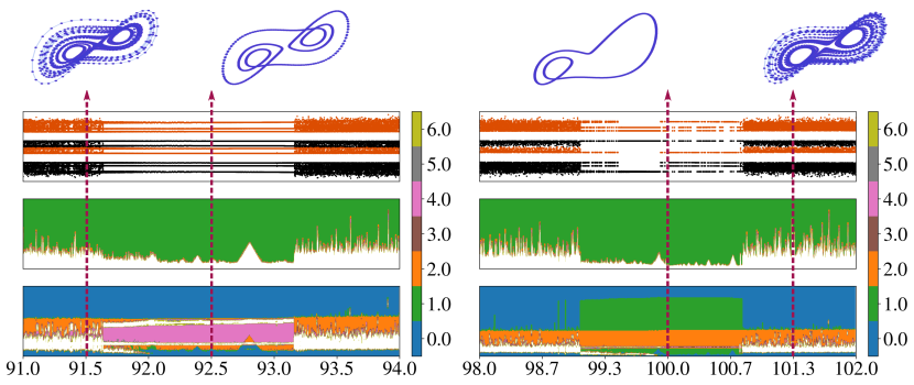
Figure 8: black Zoomed in versions of Fig. 7 showing that the 1-dimensional CROCKER plot can detect changes in behavior related to different sorts of looping structures which were harder to detect using the Lyapunov exponent shown in Fig. 1.

III.4 Correlation between the maximum Lyapunov exponents and the $L_{1}$ norm of CROCKER plots

We have shown a close relationship in terms of the Pearson correlation coefficient for both the Rössler and Lorenz systems; to see if this behavior persists, in this section we show similar tests for a larger collection of dynamical systems. Specifics for the systems and their simulation information are given in Appendix D. In Table 1, we show both the Pearson $r$ and Spearman $\rho$ correlation coefficients with subscripts denoting the dimension of CROCKER plots used black in each algorithm. Details of $r$ and $\rho$ can be found in Appendix C.

From Table 1, we can conclude, at least experimentally, that the correlation between the maximal Lyapunov exponent and 1- dimensional $L_{1}$ norm of CROCKER is a strong positive linear. black The correlation coefficients between the maximum Lyapunov exponent came from the Benettin algorithm and $L_{1}$ norm of Betti vectors is greater than the one obtained from Rösenstein algorithm. It shows that the $L_{1}$ norms of Betti vectors includes more information than Rösenstein algorithm when we do not have the full equations of the model. For completeness, the appendix (Fig. 12) includes the bifurcation diagrams and CROCKER plots for the dynamical systems given in Table 1 in Appendix D.

Table 1: black The Spearman $\rho$ and Pearson $r$ correlation between the maximum Lyapunov exponent, obtained from Rösenstein and Benettin algorithm, and $L_{1}$ norm of Betti vectors for each dimension 0 and 1.

	Rösenstein Algorithm					Benettin Algorithm
Systems	$\rho_{0}$	$r_{0}$	$\rho_{1}$	$r_{1}$		$\rho_{0}$	$r_{0}$	$\rho_{1}$	$r_{1}$
Lorenz	$0.679$	$0.854$	$0.647$	$\mathbf{0.857}$		$0.657$	$\mathbf{0.936}$	$0.622$	$0.934$
Rössler	$\mathbf{0.863}$	$0.856$	$0.797$	$0.823$		$\mathbf{0.884}$	$0.88$	$0.807$	$0.847$
Coupled Lorenz Rössler	$0.924$	$\mathbf{0.925}$	$0.887$	$0.878$		$0.912$	$\mathbf{0.937}$	$0.874$	$0.892$
Complex butterfly	$0.934$	$0.942$	$0.932$	$\mathbf{0.945}$		$0.927$	$0.948$	$0.912$	$\mathbf{0.953}$
Hadley circulation	$0.805$	$0.861$	$0.832$	$\mathbf{0.871}$		$0.816$	$0.884$	$0.841$	$\mathbf{0.892}$
Moore-Spiegel	$0.592$	$\mathbf{0.841}$	$0.593$	$0.808$		$0.572$	$\mathbf{0.863}$	$0.563$	$0.845$
Halvorsens	$0.737$	$0.857$	$0.745$	$\mathbf{0.888}$		$0.731$	$0.865$	$0.71$	$\mathbf{0.897}$
Burke-Shaw	$0.805$	$0.843$	$0.823$	$\mathbf{0.859}$		$0.815$	$0.833$	$0.833$	$\mathbf{0.873}$
Rucklidge	$0.842$	$\mathbf{0.934}$	$0.835$	$0.928$		$0.852$	$\mathbf{0.942}$	$0.832$	$0.933$
WINDMI	$0.787$	$0.896$	$0.789$	$\mathbf{0.916}$		$0.789$	$0.898$	$0.802$	$\mathbf{0.921}$

III.5 Computation Cost

We further note the computational cost of each method black in the setting where we assume the input data is available but the model is not. For this purpose, we first simulate the solution of the dynamical system using the python library teaspoon Myers et al. (2020). We then record the computation time of two methods starting from the input of the available data: (i) $L_{1}$ norms of Betti vectors and (ii) the maximum Lyapunov exponent computed used Rösenstein algorithm. All computations were performed on a Ubuntu 20.10 desktop with 16 GB RAM, Intel(R) Core(TM) i7-9700 CPU 3.00GHz, and 8 cores using the python language. A table of computation times for the dynamical systems defined in Appendix D is given in Table 2. These calculations are done for 600 bifurcation parameter values; the average and standard deviation of the run times is shown. Computation for determining $\|Bv_{i}\|_{1}$ is time from input of point cloud to output of $L_{1}$ norm; and so includes subsampling, construction of the simplicial complex filtration, persistence diagram, Betti vector, and computation of the norm. Lyapunov code was performed using the slope of the average divergence black curves obtained from linear fits as described black in the original Rösenstein paperRösenstein, Collins, and De Luca (1993). To get comparable execution time, we fixed the number of divergences are calculated to be in the range of the linear region, as first 20 distances in the calculation of the maximum Lyapunov exponent. We note that in most cases the run time for the topological representations is comparable with the Lyapunov exponent computation, and in many cases is actually considerably faster. These computations were performed largely with out-of-the-box open source software; we suspect that computations can be sped up with more attention paid to code developed specifically for this purpose.

Table 2: For each system defined in Appendix D, we record the execution time to obtain black the maximum Lyapunov exponents used the Rösenstein algorithm and the $L_{1}$ norm of Betti vectors for each particular system parameter.

Systems	Lyapunov	$\mathbf{\|Bv_{0}\|_{1}}$	$\mathbf{\|Bv_{1}\|_{1}}$
Lorenz	0.42 $\pm$ 0.47	0.53 $\pm$ 0.56	0.51 $\pm$ 0.69
Rossler	1.07 $\pm$ 0.71	1.21 $\pm$ 1.86	0.98 $\pm$ 1.08
Coupled Lorenz Rossler	0.38 $\pm$ 0.35	1.24 $\pm$ 1.88	1.12 $\pm$ 2.04
Complex butterfly	2.52 $\pm$ 1.15	0.36 $\pm$ 0.31	0.33 $\pm$ 0.31
Hadley circulation	2.83 $\pm$ 1.03	1.24 $\pm$ 1.51	1.21 $\pm$ 1.49
Moore-Spiegel	2.47 $\pm$ 0.91	0.34 $\pm$ 0.34	0.28 $\pm$ 0.12
Halvorsens	2.49 $\pm$ 0.92	1.09 $\pm$ 0.81	1.19 $\pm$ 1.69
Burke-Shaw	2.73 $\pm$ 2.31	1.35 $\pm$ 0.92	1.41 $\pm$ 1.39
Rucklidge	2.36 $\pm$ 1.21	0.79 $\pm$ 0.79	0.91 $\pm$ 1.09
WINDMI	1.97 $\pm$ 0.52	0.63 $\pm$ 0.43	0.78 $\pm$ 0.55

IV Conclusions and future directions

In this work, we have begun an investigation of the use of CROCKER plots for bifurcation analysis in dynamical systems. We show that in a simple test case, there is clearly a relationship between a representation of change in the system (the Lyapunov exponent) with the structure of the CROCKER plot, as well as with the $L_{1}$ norm of each Betti vector. We also proved a relationship between the 1-Wasserstein distance to the empty diagram, and the $L_{1}$ norm of the Betti vector.

This work, of course, leads to many interesting open questions. For starters, all work in this paper has been done in a data-driven manner. We suspect more can be done to provide a theoretical connection between the Lyapunov exponent and the $L_{1}$ norm of the Betti curve.

Further, while our computation times are black on par with those for computing Lyapunov, we believe more can be done to improve black the computation time of the method as shown. First, to our knowledge all TDA code available computes Betti vectors by first computing the full persistence diagram, and then reverse engineering the Betti curve. Might there be a more direct computation method which provides speedups relative to the desired refinement of the partition?

Another potentially useful aspect of the CROCKER method for analyzing chaos as opposed to Lyapunov exponents is that of sensitivity to noise. In particular, Lyapunov is notorious for its slow computation and its sensitivity to error and noise. On the other hand, persistence comes with a theoretically grounded framework showing stability to noisy systems; i.e. that the construction of persistence from input data is a 1-Lipschitz procedure. The issue to be overcome is that the instability of Betti numbers Xian et al. (2022); Johnson and Jung (2021) extends to the CROCKER plots. That being said, our Prop. II.1 shows that the construction of Betti curves is a continuous procedure. Further work, either data driven or theoretical, is needed to understand whether this instability shows up in the cases of the embedded time series data being studied in this paper.

Author Declarations

Conflict of Interest

The authors have no conflicts to disclose.

Data Availability

The data that support the findings of this study are available from the corresponding author upon reasonable request.

black

Appendix A Benettin vs. Rösenstein’s Algorithms for Maximal Lyapunov Exponents

In this section, we give further information on the differences between the Benettin and Rösenstein algorithms for computing maximal Lyapunov exponents. For more information on the maximum Lyapunov exponent, we refer the reader to Kantz and Schreiber’s book Kantz and Schreiber (2003) and Parlitz’s notes Parlitz (2016).

The main difference between the two algorithms is as follows. The Rösenstein algorithm can be computed using only a reconstructed attractor from a dynamical system without necessarily having access to the underlying differential equations. In this case, the goal is to determine the slope of the average divergence curve and shown in Fig. 9(b).

The issue that arises is that manual input is required. The approximation for the maximum Lyapunov exponent is the slope of a fit to the initial portion of the curve. If we are lucky and choose $k=25$, we see that the fitted yellow line gives a reasonable approximation to the slope of the initial portion. However, if we instead choose $k=40$, the fitted line is no longer a reasonable estimate. The solution is, in fact, to manually check all input time series, however, for the large number of realizations studied in this manuscript, this is unreasonable to do beyond basic spot checking. All calculations used in the main manuscript use $k=20$, which was chosen as it seems to give reasonable results.

On the other hand, if we are in a situation where we have access to the model information, a better choice of Lyapunov computation is Benettin’s algorithm. This works by evolving the tangent vectors and following the Gram-Schmidt procedure which requires the Jacobian matrix of the system. For this reason, we treat the Benettin calculation as the ground truth in this manuscript, but provide results with comparison to the Rösenstein algorithm since this is a commonly used tool in practice when the model is not available.

In Fig. 9(a), we have plotted some example computations, where each point represents the maximal Lyapunov exponent for the same realization of the Rössler system using the two methods. In one case, every computation uses $k=25$ and in the other, $k=40$. While there is some noise in the approximation, which is to be expected, we see that Rösenstein is close to a linear fit with the Benettin results. The MSE for these lines are $1.3\times 10^{-6}$ and $3\times 10^{-6}$, respectively. Note that the outlier point drawn as a red star is the example used to calculate Fig. 9(b).

Note that while the results differ by a multiplicative constant, the only thing that matters for analysis is whether the exponent is zero or non-zero, thus showing that the automated parameter choices (in particular, $k$) we have made are reasonable. It will be interesting to see in future work how much dependence there is on the results of the correlation between the TDA results and those using different choices of $k$.

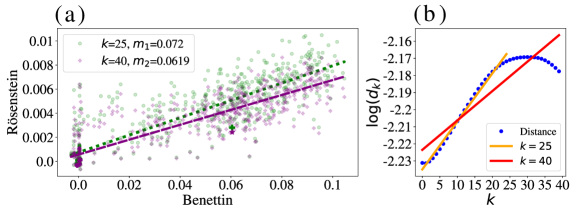
Figure 9: The relationship between two methods, Rösenstein and Benettin algorithm, to calculate the maximum Lyapunov exponent for the different 600 Rössler systems. Figure (a) shows nearly the linear relation between them for two different choices of $k$ in the Rösenstein algorithm. Figure (b) shows the last step of Rösenstein algorithm to calculate the maximum Lyapunov exponent corresponding to the same system realization shown as the purple star and green plus sign in the scatter plot at left.

Appendix B Relation between Wasserstein distance and Betti curves

In this section of the appendix, we give the proof of Prop. II.1, which states that the relationship between the norm of the Betti curve and the 1-Wasserstein distance are related as follows.

See II.1

First, we note that because the Betti curve is an integer valued function, we can rewrite it in terms of indicator functions of each bar in the barcode. Specifically, let $D=\{\alpha_{i}=(b_{i},d_{i})\}_{i=0}^{w}$ be a persistence diagram with $|D|=w+1$ points. The Betti curve of the persistence diagram $B_{D}:\mathbb{R}\rightarrow\mathbb{N}$ is given by

$$B_{D}(s)=\sum_{\alpha\in D}\mathds{1}_{\alpha}(s),$$ (2)

where the indicator function for a point $\alpha=(b,d)\in D$ is

$$\mathds{1}_{\alpha}(s)=\begin{cases}1,\quad b\leq s<d,\\ 0,\quad\mbox{otherwise}.\end{cases}$$

See, for example, the Betti curve given in Fig. 10.

On the other hand, we can obtain the topological features by using 1-Wasserstein distance between a given diagram $D$ and the empty diagram $D_{\emptyset}$. Using Defn. II.4, we have that

$$W_{1}(D,D_{\emptyset})=\frac{1}{2}\sum_{\alpha\in D}\ell_{\alpha},$$ (3)

where $\ell_{\alpha}=d-b$ is the lifetime of the topological feature $\alpha=(b,d)\in D$.

To prove Prop. II.1, we begin with the following lemma, which will be set up to prove the proposition by induction.

Lemma B.1.

Let $D=\{\alpha_{i}=(b_{i},d_{i})\}_{i=0}^{w}$ be persistence diagram and let $A$ be the maximum value of the Betti curve, $a=\max_{s\in\mathbb{R}}B_{D}(s)$. Let $\overline{\alpha}_{*}$ be a maximal (with respect to inclusion) connected interval where $B_{D}$ takes value $A$, i.e. $B_{D}(s)=A$ for all $s\in\overline{\alpha}_{*}.$ Then there is a persistence diagram $\widetilde{D}$ which contains $\overline{\alpha}_{*}$ as a bar, has the same number of bars as $D$, and satisfies

$$W_{1}(D,D_{\emptyset})=W_{1}(\tilde{D},D_{\emptyset})\quad\mbox{ and }\quad B_{D}(s)=B_{\tilde{D}}(s).$$

Proof.

If $\overline{\alpha}_{*}$ is already a bar of $D$, we set $\widetilde{D}=D$ to complete the proof, so we may assume that there is no such bar in $D$. This means that there must be two bars corresponding to the endpoints of the interval. Then let $\alpha_{1}=(b_{1},d_{1})$ and $\alpha_{2}=(b_{2},d_{2})$ be bars in $D$ with $b_{1}<b_{2}=b_{*}<d_{*}=d_{1}<d_{2}$. See Fig. 10 for an example of the two cases.

Define $\alpha_{1}^{\prime}=(b_{2},d_{1})$ and $\alpha_{2}^{\prime}=(b_{1},d_{2})$ to be a pair of bars with traded endpoints and let $\tilde{D}=D\backslash\{\alpha_{1},\alpha_{2}\}\cup\{\alpha_{1}^{\prime},\alpha_{2}^{\prime}\}$ be the diagram with those bars swapped in. Then because the lifetimes satisfy

$$\ell_{\alpha_{1}}+\ell_{\alpha_{2}} =(d_{1}-b_{1})+(d_{2}-b_{2})$$

$$=(d_{1}-b_{2})+(d_{2}-b_{1})$$

$$=\ell_{\alpha_{1}^{\prime}}+\ell_{\alpha_{2}^{\prime}}$$

we have that

$$W_{1}(D,D_{\emptyset})=\frac{1}{2}\sum_{\alpha\in D}\ell_{\alpha}= \frac{1}{2}\left(\ell_{\alpha_{1}}+\ell_{\alpha_{2}}\right)+\frac{1}{2}\sum_{\alpha\in D\backslash\{\alpha_{1},\alpha_{2}\}}\ell_{\alpha},$$

$$= \frac{1}{2}\left(\ell_{\alpha_{1}^{\prime}}+\ell_{\alpha_{2}^{\prime}}\right)+\frac{1}{2}\sum_{\alpha\in D\backslash\{\alpha_{1},\alpha_{2}\}}\ell_{\alpha},$$

$$= W_{1}(\tilde{D},D_{\emptyset}).$$

It is easy to check that $\mathds{1}_{\alpha_{1}}(s)+\mathds{1}_{\alpha_{2}}(s)=\mathds{1}_{\overline{\alpha}_{1}}(s)+\mathds{1}_{\overline{\alpha}_{2}}(s).$ Combining this with Eqn. 2, we have

$$B_{D}(s)=\sum_{\alpha\in D}\mathds{1}_{\alpha}(s)= \mathds{1}_{\alpha_{1}}(s)+\mathds{1}_{\alpha_{2}}(s)+\sum_{\alpha\in D\backslash\{\alpha_{1},\alpha_{2}\}}\mathds{1}_{\alpha}(s),$$

$$= \mathds{1}_{\overline{\alpha}_{1}}(s)+\mathds{1}_{\overline{\alpha}_{2}}(s)+\sum_{\alpha\in D\backslash\{\alpha_{1},\alpha_{2}\}}\mathds{1}_{\alpha}(s),$$

$$= B_{\tilde{D}}(s)$$

completing the proof. ∎

For simple visualization example, consider Figure 10. In both example barcodes, we have $\alpha_{*}=[b_{2},d_{1})$. In Fig. 10(a) the two bars correspond to $\alpha_{1}$ and $\alpha_{2}$, and when endpoints are swapped, result in the bars $\alpha_{1}^{\prime}$ and $\alpha_{2}^{\prime}$ in Fig. 10(b). However, the Betti curve shown in Fig. 10(c) remains the same for both.

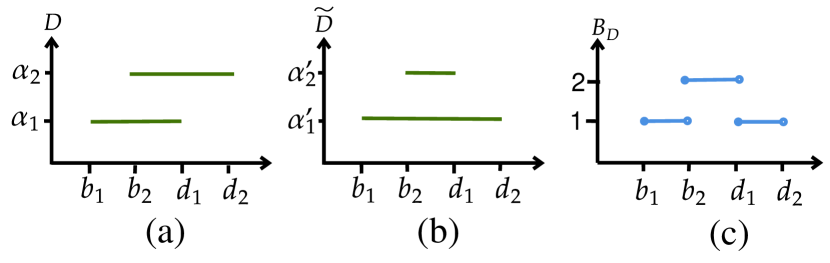
Figure 10: An example of two barcodes (panels (a) and (b)) with the same Betti curve (panel (c)) as constructed in Lem. B.1.

We can now use the above lemma in the inductive step of the proof of the main proposition.

Proof of Proposition II.1 .

We will prove the statement by induction on the number of bars $k$ of a given diagram.

Since the case of the empty diagram is vacuously true, we will start with the base case $w=1$ for clarity. This is visualized in Fig. 11. A diagram with a single bar $(s_{0},s_{1})$ shown in Fig. 11(a), and the Betti curve is given in Fig. 11(b). Then the area under the curve is $\int_{\mathbb{I}}B_{D_{1}}(s)\ ds=s_{1}-s_{0}$. On the other hand, the 1-Wasserstein distance to the empty diagram, as shown in Fig. 11(c), the distance is the half lifetime of the topological feature, thus $\tfrac{1}{2}(s_{0},s_{1})$. So,

$$\int_{\mathbb{I}}B_{D_{1}}(s)\ ds=(s_{1}-s_{0})\cdot 1=2\cdot\frac{s_{1}-s_{0}}{2}=2\cdot W_{1}(D_{1},D_{\emptyset})\ .$$

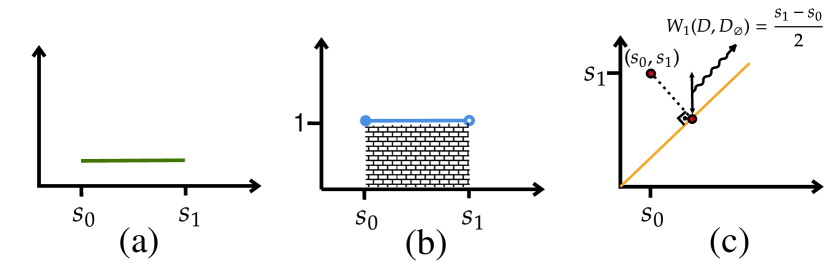
Figure 11: (a) Persistence barcodes, (b) Betti curve and (c) persistence diagram with Wasserstein distances for the example of a diagram with a single point.

Now we assume the statement is true for a diagram with $w$ bars. Assume that we have a persistence diagram $D$ with $w+1$ bars and let $\widetilde{D}$ be the diagram obtained from Lem. B.1 with bar $\alpha_{*}=(b_{*},d_{*})\in\widetilde{D}$. Let $\widetilde{D}_{w}$ be the diagram $\widetilde{D}$ with that bar removed, i.e. $\widetilde{D}_{w}\cup\{\alpha_{*}\}=\widetilde{D}$ and note that $|D_{w}|=w$. Then we have

$$\int_{\mathbb{I}}B_{D}(s)\ ds= \int_{\mathbb{I}}B_{\widetilde{D}}(s)\ ds$$ (Lem. B.1)

$$= \int_{\mathbb{I}}B_{\widetilde{D}_{w}}(s)\ ds+\int_{\mathbb{I}}\mathds{1}_{\alpha_{*}}(s)\ ds$$

$$= 2\cdot W_{1}(\widetilde{D}_{w},D_{\emptyset})+(\widetilde{d}_{*}-\widetilde{b}_{*})$$ (induction)

$$= 2\cdot W_{1}(\widetilde{D},D_{\emptyset})$$ (Defn. 3)

$$= 2\cdot W_{1}(D,\emptyset)$$ (from Lemma B.1)

completing the proof. ∎

Appendix C Pearson and Spearman Correlations

The Pearson correlation coefficient $r\in[-1,1]$ measures the linear correlation of two series $x$ and $y$. The Pearson correlation coefficient for two datasets is calculated as

$$r=\frac{\sum_{i=1}^{n}\left(x_{i}-\bar{x}\right)\left(y_{i}-\bar{y}\right)}{\sqrt{\sum_{i=1}^{n}\left(x_{i}-\bar{x}\right)^{2}}\sqrt{\sum_{i=1}^{n}\left(y_{i}-\bar{y}\right)^{2}}}.$$ (4)

The coefficient $r$ indicates a perfect positive or negative linear correlation when $r=1$ or $r=-1$, respectively, while $r=0$ represents no linear correlation. However Pearson correlation is limited in that it can only discover linear associations.

To investigate nonlinear associations, one may consider Spearman’s correlation which is the non-parametric version of the Pearson correlation. Spearman’s correlation coefficient $\rho\in[-1,1]$ is also calculated using Eq. (4) with the ordinal ranking of the variables $x$ and $y$ instead of their numerical values. This substitution allows for detecting nonlinear correlation trends to be represented as long as the correlation is monotonic.

Appendix D Dynamical System Details

In this section we give details on the various dynamical systems simulated for the experiments from Sec. III. All simulations were performed using the python package teaspoon Myers et al. (2020) with default parameters other than those noted.

D.1 Lorenz

The Lorenz system consists of three ordinary differential equations referred to as Lorenz equations:

$$\dot{x}=\sigma(y-x),\quad\dot{y}=x(\rho-z)-y,\quad\dot{z}=xy-\beta z,$$

where the parameters $\sigma=10,\>\beta=8/3$ are fixed; the control parameter $\rho$ is varied across 600 equally spaced values between 90 and 105; and the system is simulated with a sampling rate of 100 Hz for 100 seconds using the initial condition ${[x,y,z]}=[10^{-10},0,1]$. After solving the system, we take only the last 20 seconds to avoid transients.

D.2 Rössler

The Rössler system is defined as follows

$$\dot{x}=-y-z,\quad\dot{y}=x+ay,\quad\dot{z}=b+z(x-c),$$

where the parameters $b=2,\>c=4$ are fixed; the control parameter $a$ is varied across 600 equally spaced values between 0.37 and 0.43; and the system is simulated with a sampling rate of 15 Hz for 1000 seconds using the initial condition ${[x,y,z]}=[-0.4,0.6,1]$. After solving the system, we take only the last 170 seconds to avoid transients.

D.3 Coupled Lorenz Rössler

The Coupled Lorenz-Rössler system defined as follows

$$\dot{x_{1}} =-y_{1}-z_{1}+k_{1}\left(x_{2}-x_{1}\right), \dot{x_{2}} =\sigma\left(y_{2}-x_{2}\right),$$

$$\dot{y_{1}} =x_{1}+a_{2}y_{1}+k_{2}\left(y_{2}-y_{1}\right), \dot{y_{2}} =\gamma x_{2}-y_{2}-x_{2}z_{2},$$

$$\dot{z_{1}} =b_{2}+z_{1}\left(x_{1}-c_{2}\right)+k_{3}\left(z_{2}-z_{1}\right), \dot{z_{2}} =x_{2}y_{2}-b_{1}z_{2},$$

where the parameters $b_{1}=8/3,\>b_{2}=0.2,\>c_{2}=5.7,\>k_{1}=0.1,\>k_{2}=0.1$,  $k_{3}=0.1,\>{\gamma}=28,\>\sigma=10$ are fixed; the control parameter $a$ is varied across 600 equally spaced values between 0.3 and 0.5; and the system is simulated with a sampling rate of 50 Hz for 500 seconds using the initial condition $[x_{1},y_{1},z_{1},x_{2},y_{2},z_{2}]=[0.1,0.1,0.1,0,0,0]$. After solving the system, we take only the last 30 seconds to avoid transients.

D.4 Complex butterfly

The complex butterfly system is defined as follows

$$\dot{x}=a(y-x),\quad\dot{y}=2\operatorname{sgn}(x),\quad\dot{z}=|x|-1,$$

where the control parameter $a$ is varied across 600 equally spaced values between 0.10 and 0.60; and the system is simulated with a sampling rate of 10 Hz for 1000 seconds using the initial condition ${[x,y,z]}=[0.2,0,0]$. After solving the system, we take only the last 500 seconds to avoid transients.

D.5 Hadley circulation

The Hadley circulation system is defined as follows

$$\dot{x}= -y^{2}-z^{2}-ax+aF$$

$$\dot{y}= xy-bxz-y+G$$

$$\dot{z}= bxy+xz-z,$$

where the parameters $b=4,\>F=8,\>G=1$ are fixed; the control parameter $a$ is varied across 600 equally spaced values between 0.20 and 0.25; and the system is simulated with a sampling rate of 50 Hz for 500 seconds using the initial condition ${[x,y,z]}=[-10,0,37]$. After solving the system, we take only the last 80 seconds to avoid transients.

D.6 Moore-Spiegel Oscilator

The Moore-Spiegel oscilator system is defined as follows

$$\dot{x}=y,\quad\dot{y}=z,\quad\dot{z}=-z-(T-{R}+Rx^{2})y-Tx,\quad$$

where the parameter $R=20$ is fixed; the control parameter $T$ is varied across 600 equally spaced values between 7.0 and 8.0; and the system is simulated with a sampling rate of 100 Hz for 500 seconds using the initial condition ${[x,y,z]}=[0.2,0.2,0.2]$. After solving the system, we take only the last 10 seconds to avoid transients.

D.7 Halvorsens cyclically symmetric attractor

The Halvorsens cyclically symmetric attractor is defined as follows

$$\dot{x}= -ax-by-cz-y^{2}$$

$$\dot{y}= -ay-bz-cx-z^{2}$$

$$\dot{z}= -az-bx-cy-x^{2},$$

where the parameters $b=4,\>c=4$ are fixed; the control parameter $a$ is varied across 600 equally spaced values between 1.40 and 1.85; and the system is simulated with a sampling rate of 200 Hz for 200 seconds using the initial condition ${[x,y,z]}=[-5,0,0]$. After solving the system, we take only the last 25 seconds to avoid transients.

D.8 Burke-Shaw attractor

The Burke-Shaw system is defined as follows

$$\dot{x}=-s(x+y),\quad\dot{y}=-y-sxz,\quad\dot{z}=sxz+V,\quad$$

where the parameter $V=10$ is fixed; the control parameter $s$ is varied across 600 equally spaced values between 9.0 and 13.0; and the system is simulated with a sampling rate of 200 Hz for 500 seconds using the initial condition ${[x,y,z]}=[0.6,0,0]$. After solving the system, we take only the last 25 seconds to avoid transients.

D.9 Rucklidge attractor

The Rucklidge system is defined as follows

$$\dot{x}=-kx+\lambda y-yz,\quad\dot{y}=x,\quad\dot{z}=-z+y^{2},$$

where the parameter $\lambda=6.7$ is fixed; the control parameter $k$ is varied across 600 equally spaced values between 1.0 and 1.7; and the system is simulated with a sampling rate of 50 Hz for 1000 seconds using the initial condition ${[x,y,z]}=[1,0,4.5]$. After solving the system, we take only the last 100 seconds to avoid transients.

D.10 WINDMI

The WINDMI system is defined as follows

$$\dot{x}=y,\quad\dot{y}=z,\quad\dot{z}=-az-y+b-e^{x},$$

where the parameter $b=2.5$ is fixed; the control parameter $a$ is varied across 600 equally spaced values between 0.7 and 1.0; and the system is simulated with a sampling rate of 20 Hz for 1000 seconds using the initial condition ${[x,y,z]}=[1,0,4.5]$. After solving the system, we take only the last 250 seconds to avoid transients.

Appendix E CROCKER plots for other dynamical systems

In this section, we give an additional figure (Fig. 12) detailing similar results to those seen in Sec. III for the remainder of the systems mentioned in Appendix D.

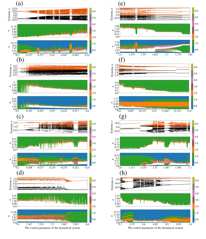
Figure 12: black The bifurcation diagram and 0- and 1- dimensional CROCKER for each dynamical system in Appendix. D. ((a)-Coupled Lorenz Rössler, (b)- Complex Butterfly, (c)- Hadley circulation, (d)- Moore-Spiegel oscilator, (e)- Halvorsens cyclically symmetric attractor, (f)-Burke-Shaw attractor, (g)- Rucklidge attractor and (h)- WINDMI)

References

- Topaz, Ziegelmeier, and Halverson (2015) C. M. Topaz, L. Ziegelmeier, and T. Halverson, “Topological data analysis of biological aggregation models,” PLOS ONE 10, 1–26 (2015).
- Robinson (2014) M. Robinson, Topological signal processing, Vol. 81 (Springer, 2014).
- Robins, Meiss, and Bradley (2000) V. Robins, J. D. Meiss, and E. Bradley, Computational topology at multiple resolutions: foundations and applications to fractals and dynamics, Ph.D. thesis, University of Colorado (2000).
- Kaczynski, Mischaikow, and Mrozek (2004) T. Kaczynski, K. Mischaikow, and M. Mrozek, Computational Homology (Springer, 2004).
- Khasawneh and Munch (2017) F. A. Khasawneh and E. Munch, “Utilizing topological data analysis for studying signals of time-delay systems,” in Time Delay Systems (Springer, 2017) pp. 93–106.
- Garland, Bradley, and Meiss (6 11) J. Garland, E. Bradley, and J. D. Meiss, “Exploring the topology of dynamical reconstructions,” Physica D: Nonlinear Phenomena 334, 49–59 (2016-11).
- Mittal and Gupta (2017) K. Mittal and S. Gupta, “Topological characterization and early detection of bifurcations and chaos in complex systems using persistent homology,” Chaos: An Interdisciplinary Journal of Nonlinear Science 27, 051102 (2017).
- Dee Algar, Corrêa, and Walker (2021) S. Dee Algar, D. C. Corrêa, and D. M. Walker, “On detecting dynamical regime change using a transformation cost metric between persistent homology diagrams,” Chaos: An Interdisciplinary Journal of Nonlinear Science 31, 123117 (2021).
- Güzel and Kaygun (2022) I. Güzel and A. Kaygun, “Classification of stochastic processes with topological data analysis,” in Proceedings of BAŞARIM 2022 - 7th High-Performance Computing Conference (BAŞARIM, 2022) arXiv:2206.03973 .
- Karan and Kaygun (2021) A. Karan and A. Kaygun, “Time series classification via topological data analysis,” Expert Systems with Applications 183, 115326 (2021).
- Maletić, Zhao, and Rajković (2016) S. Maletić, Y. Zhao, and M. Rajković, “Persistent topological features of dynamical systems,” Chaos: An Interdisciplinary Journal of Nonlinear Science 26, 053105 (2016).
- Marchese and Maroulas (2017) A. Marchese and V. Maroulas, “Signal classification with a point process distance on the space of persistence diagrams,” Advances in Data Analysis and Classification (2017), 10.1007/s11634-017-0294-x.
- Kim, Kim, and Rinaldo (2018) K. Kim, J. Kim, and A. Rinaldo, “Time series featurization via topological data analysis,” arXiv preprint arXiv:1812.02987 (2018), arXiv:1812.02987 [cs.CG] .
- Seversky, Davis, and Berger (2016) L. M. Seversky, S. Davis, and M. Berger, “On time-series topological data analysis: New data and opportunities,” in The IEEE Conference on Computer Vision and Pattern Recognition (CVPR) Workshops (2016).
- Venkataraman, Ramamurthy, and Turaga (2016) V. Venkataraman, K. N. Ramamurthy, and P. Turaga, “Persistent homology of attractors for action recognition,” in 2016 IEEE International Conference on Image Processing (ICIP) (IEEE, 2016).
- Perea and Harer (2015) J. A. Perea and J. Harer, “Sliding windows and persistence: An application of topological methods to signal analysis,” Foundations of Computational Mathematics , 1–40 (2015).
- Perea (2019) J. A. Perea, “Topological time series analysis,” Notices of the American Mathematical Society 66, 686–694 (2019).
- Berwald, Gidea, and Vejdemo-Johansson (2014) J. J. Berwald, M. Gidea, and M. Vejdemo-Johansson, “Automatic recognition and tagging of topologically different regimes in dynamical systems,” Discontinuity, Nonlinearity, and Complexity 3, 413–426 (2014).
- Tan et al. (2021) E. Tan, D. Corrêa, T. Stemler, and M. Small, “Grading your models: Assessing dynamics learning of models using persistent homology,” Chaos: An Interdisciplinary Journal of Nonlinear Science 31, 123109 (2021).
- Bubenik and Wagner (2020) P. Bubenik and A. Wagner, “Embeddings of persistence diagrams into hilbert spaces,” Journal of Applied and Computational Topology 4, 339–351 (2020).
- Yesilli et al. (2019) M. C. Yesilli, S. Tymochko, F. A. Khasawneh, and E. Munch, “Chatter diagnosis in milling using supervised learning and topological features vector,” 2019 18th IEEE International Conference On Machine Learning And Applications (ICMLA) (2019), 10.1109/ICMLA.2019.00200, special session acceptance rate: 43%, arXiv:1910.12359 .
- Khasawneh and Munch (2016) F. A. Khasawneh and E. Munch, “Chatter detection in turning using persistent homology,” Mechanical Systems and Signal Processing 70-71, 527–541 (2016).
- Khasawneh and Munch (2018) F. A. Khasawneh and E. Munch, “Topological data analysis for true step detection in periodic piecewise constant signals,” Proceedings of the Royal Society A: Mathematical, Physical and Engineering Sciences 474, 20180027 (2018).
- Gidea (2017) M. Gidea, “Topological data analysis of critical transitions in financial networks,” in 3rd International Winter School and Conference on Network Science : NetSci-X 2017 (Springer International Publishing, Cham, 2017) pp. 47–59.
- Gidea and Katz (2018) M. Gidea and Y. Katz, “Topological data analysis of financial time series: Landscapes of crashes,” Physica A: Statistical Mechanics and its Applications 491, 820–834 (2018), 1703.04385v2 .
- Gidea et al. (2020) M. Gidea, D. Goldsmith, Y. Katz, P. Roldan, and Y. Shmalo, “Topological recognition of critical transitions in time series of cryptocurrencies,” Physica A: Statistical Mechanics and its Applications 548, 123843 (2020), 1809.00695v1 .
- Rivera-Castro, Pilyugina, and Burnaev (2019) R. Rivera-Castro, P. Pilyugina, and E. Burnaev, “Topological data analysis for portfolio management of cryptocurrencies,” in 2019 International Conference on Data Mining Workshops (ICDMW) (IEEE, 2019).
- Majumdar and Laha (2020) S. Majumdar and A. K. Laha, “Clustering and classification of time series using topological data analysis with applications to finance,” Expert Systems with Applications 162, 113868 (2020).
- Ignacio et al. (2019) P. S. Ignacio, C. Dunstan, E. Escobar, L. Trujillo, and D. Uminsky, “Classification of single-lead electrocardiograms: TDA informed machine learning,” in 2019 18th IEEE International Conference On Machine Learning And Applications (ICMLA) (IEEE, 2019).
- Stolz, Harrington, and Porter (2017) B. J. Stolz, H. A. Harrington, and M. A. Porter, “Persistent homology of time-dependent functional networks constructed from coupled time series,” Chaos: An Interdisciplinary Journal of Nonlinear Science 27, 047410 (2017).
- Majumder et al. (2020) S. Majumder, F. Apicella, F. Muratori, and K. Das, “Detecting autism spectrum disorder using topological data analysis,” in ICASSP 2020 - 2020 IEEE International Conference on Acoustics, Speech and Signal Processing (ICASSP) (IEEE, 2020).
- Chung et al. (2021) Y.-M. Chung, C.-S. Hu, Y.-L. Lo, and H.-T. Wu, “A persistent homology approach to heart rate variability analysis with an application to sleep-wake classification,” Frontiers in Physiology 12 (2021), 10.3389/fphys.2021.637684.
- Emrani, Gentimis, and Krim (2014) S. Emrani, T. Gentimis, and H. Krim, “Persistent homology of delay embeddings and its application to wheeze detection,” Signal Processing Letters, IEEE 21, 459–463 (2014).
- Tymochko, Munch, and Khasawneh (2020) S. Tymochko, E. Munch, and F. A. Khasawneh, “Using zigzag persistent homology to detect hopf bifurcations in dynamical systems,” Algorithms 13, 278 (2020).
- Myers, Munch, and Khasawneh (2019) A. Myers, E. Munch, and F. A. Khasawneh, “Persistent homology of complex networks for dynamic state detection,” Physical Review E 100, 022314 (2019).
- Myers, Khasawneh, and Munch (2022) A. Myers, F. A. Khasawneh, and E. Munch, “Topological signal processing using the weighted ordinal partition network,” arXiv preprint arXiv:2205.08349 (2022), 2205.08349 .
- Bauer et al. (2020) U. Bauer, D. Hien, O. Junge, K. Mischaikow, and M. Snijders, “Combinatorial models of global dynamics: learning cycling motion from data,” arXiv preprint arXiv:2001.07066 (2020), 10.1088/1361-6544/abe834, arXiv:2001.07066 [math.DS] .
- Tempelman and Khasawneh (2020) J. R. Tempelman and F. A. Khasawneh, “A look into chaos detection through topological data analysis,” Physica D: Nonlinear Phenomena 406, 132446 (2020).
- Myers, Khasawneh, and Munch (2 05) A. Myers, F. Khasawneh, and E. Munch, “Temporal network analysis using zigzag persistence,” arXiv preprint arXiv:2205.11338 (2022-05), 2205.11338 .
- Tralie (2016) C. Tralie, “High-Dimensional Geometry of Sliding Window Embeddings of Periodic Videos,” in 32nd International Symposium on Computational Geometry (SoCG 2016), Leibniz International Proceedings in Informatics (LIPIcs), Vol. 51, edited by S. Fekete and A. Lubiw (Schloss Dagstuhl–Leibniz-Zentrum fuer Informatik, Dagstuhl, Germany, 2016) pp. 71:1–71:5.
- Tymochko et al. (2020) S. Tymochko, E. Munch, J. Dunion, K. Corbosiero, and R. Torn, “Using persistent homology to quantify a diurnal cycle in hurricane felix,” Pattern Recognition Letters 133, 137–143 (2020).
- Tralie and Perea (2018) C. J. Tralie and J. A. Perea, “(quasi) periodicity quantification in video data, using topology,” SIAM Journal on Imaging Sciences 11, 1049–1077 (2018).
- Levanger et al. (2019) R. Levanger, M. Xu, J. Cyranka, M. F. Schatz, K. Mischaikow, and M. Paul, “Correlations between the leading lyapunov vector and pattern defects for chaotic rayleigh-bénard convection,” Chaos: An Interdisciplinary Journal of Nonlinear Science 29, 053103 (2019).
- Wu and Hargreaves (2021) C. Wu and C. A. Hargreaves, “Topological machine learning for multivariate time series,” Journal of Experimental & Theoretical Artificial Intelligence 34, 311–326 (2021).
- Kim and Mémoli (2021) W. Kim and F. Mémoli, “Spatiotemporal persistent homology for dynamic metric spaces,” Discrete & Computational Geometry 66, 831–875 (2021).
- Cohen-Steiner, Edelsbrunner, and Morozov (2006) D. Cohen-Steiner, H. Edelsbrunner, and D. Morozov, “Vines and vineyards by updating persistence in linear time,” in Proceedings of the twenty-second annual symposium on Computational geometry (2006) pp. 119–126.
- Ulmer, Ziegelmeier, and Topaz (2019) M. Ulmer, L. Ziegelmeier, and C. M. Topaz, “A topological approach to selecting models of biological experiments,” PLOS ONE 14, 1–18 (2019).
- Bhaskar et al. (2019) D. Bhaskar, A. Manhart, J. Milzman, J. T. Nardini, K. M. Storey, C. M. Topaz, and L. Ziegelmeier, “Analyzing collective motion with machine learning and topology,” Chaos: An Interdisciplinary Journal of Nonlinear Science 29, 123125 (2019).
- Xian et al. (2022) L. Xian, H. Adams, C. M. Topaz, and L. Ziegelmeier, “Capturing dynamics of time-varying data via topology,” Foundations of Data Science 4, 1–36 (2022).
- Güzel, Munch, and Khasawneh (2022) I. Güzel, E. Munch, and F. Khasawneh, “A case study on identifying bifurcation and chaos with CROCKER plots,” in Proceedings of TDA at SDM (SIAM Data Mining), edited by R. W. R. Darling, J. A. Emanuello, E. Purvine, and A. Ridley, SIAM Data Mining (arXiv Proceedings, 2022) 2204.06321 .
- Kantz and Schreiber (2003) H. Kantz and T. Schreiber, Nonlinear Time Series Analysis, 2nd ed. (Cambridge University Press, 2003).
- Hirsch, Smale, and Devaney (2013) M. W. Hirsch, S. Smale, and R. L. Devaney, Differential equations, dynamical systems, and an introduction to chaos, 3rd ed. (Elsevier/Academic Press, Amsterdam, 2013) pp. xiv+418.
- Baker and Gollub (1996) G. L. Baker and J. P. Gollub, Chaotic dynamics: an introduction (Cambridge university press, 1996).
- Sayama (2015) H. Sayama, Introduction to the modeling and analysis of complex systems (Open SUNY Textbooks, 2015).
- Lorenz (1963) E. N. Lorenz, “Deterministic nonperiodic flow,” Journal of atmospheric sciences 20, 130–141 (1963).
- Datseris (2018) G. Datseris, “Dynamicalsystems.jl: A julia software library for chaos and nonlinear dynamics,” Journal of Open Source Software 3, 598 (2018).
- Bezanson et al. (2017) J. Bezanson, A. Edelman, S. Karpinski, and V. B. Shah, “Julia: A fresh approach to numerical computing,” SIAM review 59, 65–98 (2017).
- Benettin et al. (1980) G. Benettin, L. Galgani, A. Giorgilli, and J.-M. Strelcyn, “Lyapunov characteristic exponents for smooth dynamical systems and for hamiltonian systems; a method for computing all of them. part 1: Theory,” Meccanica 15, 9–20 (1980).
- Rösenstein, Collins, and De Luca (1993) M. T. Rösenstein, J. J. Collins, and C. J. De Luca, “A practical method for calculating largest lyapunov exponents from small data sets,” Physica D: Nonlinear Phenomena 65, 117–134 (1993).
- Dey and Wang (2022) T. K. Dey and Y. Wang, Computational Topology for Data Analysis (Cambridge University Press, 2022).
- Oudot (2017) S. Y. Oudot, Persistence Theory: From Quiver Representations to Data Analysis (Mathematical Surveys and Monographs) (American Mathematical Society, 2017).
- Munch (2017) E. Munch, “A user’s guide to topological data analysis,” Journal of Learning Analytics 4 (2017).
- Hatcher (2002) A. Hatcher, Algebraic Topology (Cambridge University Press, 2002).
- Munkres (1984) J. R. Munkres, Elements of Algebraic Topology (Addison Wesley, 1984).
- Johnson and Jung (2021) M. Johnson and J.-H. Jung, “Instability of the betti sequence for persistent homology and a stabilized version of the betti sequence,” Journal of The Korean Society For Industrial and Applied Mathematics 25, 296–311 (2021).
- Chung and Lawson (2022) Y.-M. Chung and A. Lawson, “Persistence curves: A canonical framework for summarizing persistence diagrams,” Advances in Computational Mathematics 48, 1–42 (2022).
- Cohen-Steiner et al. (2010) D. Cohen-Steiner, H. Edelsbrunner, J. Harer, and Y. Mileyko, “Lipschitz functions have -stable persistence,” Found. Comput. Math. 10, 127–139 (2010).
- Skraba and Turner (2020) P. Skraba and K. Turner, “Wasserstein stability for persistence diagrams,” (2020), arXiv:2006.16824 [math.AT] .
- Carlsson and Zomorodian (2009) G. Carlsson and A. Zomorodian, “The theory of multidimensional persistence,” Discrete & Computational Geometry 42, 71–93 (2009).
- Note (1) The naming convention comes from the association to Betti number information, but might only be obvious to those who regularly shop in US grocery stores.
- Cavanna, Jahanseir, and Sheehy (2015) N. J. Cavanna, M. Jahanseir, and D. R. Sheehy, “A geometric perspective on sparse filtrations,” arXiv preprint arXiv:1506.03797 (2015).
- Tralie, Saul, and Bar-On (2018) C. Tralie, N. Saul, and R. Bar-On, “Ripser.py: A lean persistent homology library for python,” The Journal of Open Source Software 3, 925 (2018).
- Note (2) Every 0-dimensional diagram for a point cloud has an infinite bar representing the first connected component which is born and is considered to live for every value of . Thus the 0-dimensional CROCKER plots always have a region of 1 at their maximum boundary.
- Myers et al. (2020) A. D. Myers, M. Yesilli, S. Tymochko, F. Khasawneh, and E. Munch, “Teaspoon: A comprehensive python package for topological signal processing,” in NeurIPS 2020 Workshop on Topological Data Analysis and Beyond (2020).
- Parlitz (2016) U. Parlitz, “Estimating lyapunov exponents from time series,” in Chaos Detection and Predictability, edited by C. H. Skokos, G. A. Gottwald, and J. Laskar (Springer Berlin Heidelberg, Berlin, Heidelberg, 2016) pp. 1–34.