Apsidal Alignment and Anti-Alignment of Planets in Mean-Motion Resonance: Disk-Driven Migration and Eccentricity Driving

Abstract

Planets migrating in their natal discs can be captured into mean-motion resonance (MMR), in which the planets’ periods are related by integer ratios. Recent observations indicate that planets in MMR can be either apsidally aligned or anti-aligned. How these different configurations arise is unclear. In this paper, we study the MMR capture process of migrating planets, focusing on the property of the apsidal angles of the captured planets. We show that the standard picture of MMR capture, in which the planets undergo convergent migration and experience eccentricity damping due to planet-disc interactions, always leads to apsidal anti-alignment of the captured planets. However, when the planets experience eccentricity driving from the disc, apsidally aligned configuration in MMR can be produced. In this configuration, both planets’ resonance angles circulate, but a “mixed” resonance angle librates and traps the planets near the nominal resonance location. The MMR capture process in the presence of disc eccentricity driving is generally complex and irregular, and can lead to various outcomes, including apsidal alignment and anti-alignment, as well as the disruption of the resonance. We suggest that the two resonant planets in the K2-19 system, with their moderate eccentricities and aligned apsides, have experienced eccentricity driving from their natal disc in the past.

1 Introduction

Even before the first detection of exoplanets, it was recognized that planets can migrate from their initial birth positions due to interactions with their natal protoplanetary disks (PPDs; Lin & Papaloizou, 1979; Goldreich & Tremaine, 1979, 1980, see Nelson 2018 for review). The speed and direction of migration depends on the disc density and temperature profiles. While planet-disc interactions typically circularize the planet’s orbit, eccentricity excitation can also occur under some circumstances. Goldreich & Sari (2003) demonstrated how Lindblad and corotation resonances compete to either drive or damp a giant planet’s eccentricity. More recently, Teyssandier & Ogilvie (2017) and Ragusa et al. (2017) found that, in long-term ($\geq 10^{4}$ orbits) hydrodynamic simulations, the eccentricity of a large, gap-opening planet exhibits growth and decay as the system evolves. Romero et al. (2021) found that luminous, super-earth mass protoplanets can be driven to eccentricities beyond the disk’s aspect ratio through a thermal back-reaction effect from the perturbed gas disk.

As two planets undergo differential migrations in the PPD, they may encounter mean-motion resonance (MMR), where the planets’ periods are related by integer period ratios $j:j+k$. For sufficiently slow, convergent migration, the mutual gravitational interaction between the planets can lead to MMR capture. The period ratio distribution of super-Earths/mini-Neptunes discovered by the Kepler mission indeed shows an excess of planet pairs near MMRs, although the observed MMR occurrence rate is much lower than the MMR capture rate predicted using the simplest migration/capture model. The “near MMR” systems typically have period ratios slightly larger (by 1-2%) than exact resonance (e.g. Fabrycky et al., 2014). These discrepancies could be explained by the instability of the captured state during disk-driven migration (Goldreich & Schlichting, 2014; Deck & Batygin, 2015; Delisle et al., 2015; Xu & Lai, 2016; Xu et al., 2018), resonance repulsion due to tidal eccentricity damping or planet-disk interactions (Lithwick & Wu, 2012; Batygin & Morbidelli, 2013; Delisle & Laskar, 2014; Choksi & Chiang, 2020), late-time dynamical instability (Izidoro et al., 2017), and/or outward (divergent) migration due to planetesimal scatterings (Chatterjee & Ford, 2015).

An interesting property of MMR capture concerns the relative apsidal angle $\Delta\varpi=\varpi_{1}-\varpi_{2}$ of the captured planets. For the first-order MMR ($j:j+1$), the two resonant angles are

$$\theta_{1} =(j+1)\lambda_{2}-j\lambda_{1}-\varpi_{1},$$ (1)

$$\theta_{2} =(j+1)\lambda_{2}-j\lambda_{1}-\varpi_{2},$$ (2)

where $\lambda_{1}$ and $\lambda_{2}$ are the mean longitudes of the planets. In equilibrium, we expect $\theta_{1}$ and $\theta_{2}$ to be either $0^{\circ}$ or $180^{\circ}$, implying $\Delta\varpi=0^{\circ}$ or $180^{\circ}$. As we will see in Section 2, the conventional treatment of migration and resonance capture in PPDs always produces apsidal anti-alignment when the planet’s eccentricity is damped by the disk.

Only a handful of systems in or near resonance have constrained measurements of $\Delta\varpi$, and, indeed, most exhibit apsidal anti-alignment ($\varpi=180^{\circ}$). Kepler-88 hosts two planets, b and c, near the 1:2 resonance with periods 10.9 d and 22.3 d and masses $214M_{\oplus}$ and $9.5M_{\oplus}$, respectively (Weiss et al., 2020). Kepler-9b and c are two sub-Jupiter mass planets ($M_{b}=0.25M_{J}$ and $M_{c}=0.17M_{J}$) orbiting near the 1:2 MMR ($P_{b}=19.2$ d and $P_{c}=38.9$ d; Holman et al., 2010). Both of these systems are constrained by their photodynamical data to have $\Delta\varpi\approx 180^{\circ}$ (Antoniadou & Libert, 2020). The system K2-24 has two approximately Neptune-mass planets ($M_{b}=19M_{\oplus}$, $M_{c}=15.4M_{\oplus}$), K2-24b and c, near the 1:2 resonance with periods $P_{b}=20.8$ d and $P_{c}=42.3$ d (Petigura et al., 2018). The observations of K2-24 are consistent with either the apsidally aligned or anti-aligned configuration (Antoniadou & Libert, 2020).

The only aligned system detected thus far is K2-19, a three planet system around a K dwarf star ($M=0.88M_{\odot}$; Armstrong et al., 2015). The planets K2-19b and c are near the 2:3 period ratio ($P_{b}=7.9$ d, $P_{c}=11.9$ d), and planet K2-19d lies on an orbit interior to the other two at $P_{d}=2.5$ d. Their masses are $M_{d}<10M_{\oplus}$, $M_{b}=32.4M_{\oplus}$, and $M_{c}=10.8M_{\oplus}$, with radii $R_{d}\approx 1.1R_{\oplus}$, $R_{b}\approx 7.0R_{\oplus}$, and $R_{c}\approx 4.1R_{\oplus}$. The K2-19 photometry data indicates that the innermost planet has $e_{d}\simeq 0$, planets b and c have moderate eccentricities, and $e_{b}\approx e_{c}\approx 0.2$. Their apsidal angles are constrained to within a few degrees of 0^∘ (Petigura et al., 2020; Petit et al., 2020). The origin of this alignment is unclear.

Investigating how the two planets in K2-19 could have formed with $\Delta\varpi=0^{\circ}$ through resonance capture and mutual migration (while other systems have $\Delta\varpi=180^{\circ}$) may offer us new insight into its dynamical history as well as a better understanding of the genesis of extrasolar orbital configurations in general. In this paper, we study the apsidal property of planets in MMRs produced by disk-driven migration. In Section 2, we present the standard picture of resonant capture and explore the parameter space for the coupling between the planets and the protoplanetary disk. We show that as long as the disk damps the planetary eccentricity, MMR capture always leads to apsidal anti-alignment. In Section 3, we explore the apsidal property for a test particle in the vicinity of the MMR with an eccentric planet’s MMR. These results guide our analysis in Section 4, where we show that when planet-disc interaction drives the planet’s eccentricity toward a finite, non-zero value, apsidal alignment can be produced under certain circumstances. We conclude in Section 5.

2 Disk-Driven MMR Capture: Standard Apsidal Architecture

Consider two planets with masses $m_{1}$ and $m_{2}$ orbiting a star of mass $M$ (set to 1$M_{\odot}$ throughout this paper) with semimajor axes $a_{1}$ and $a_{2}$ ($>a_{1}$) in a gaseous disk. At low eccentricities, the orbital decay rate and eccentricity damping rate due to planet-disc interactions are given by

$$\frac{\dot{a}_{i}}{a_{i}} =-\frac{1}{T_{m,i}}-\frac{2e_{i}^{2}}{T_{e,i}},$$ (3)

$$\frac{\dot{e}_{i}}{e_{i}} =-\frac{1}{T_{e,i}},$$ (4)

for each planet ($i=1,2$). For low-mass planets undergoing type-I migration and typical disc profiles, we have (Tanaka & Ward, 2004; Cresswell & Nelson, 2008)

$$T_{e,i} \sim\frac{M^{2}}{\Sigma a_{i}^{2}m}h^{4}n_{i}^{-1},$$ (5)

$$|T_{m,i}| \simeq\frac{T_{e}}{3.46h^{2}},$$ (6)

where $a_{i}$ is the semimajor axis (SMA), $\Sigma$ is the disc surface density, $h$ is the aspect ratio of the disk, and $n_{i}$ is the mean motion. Note that $T_{e,1}/T_{e,2}=m_{2}/m_{1}=1/q$. Throughout the paper, we treat $T_{e,1}$ and $T_{e,2}$ as constants (independent of the semimajor axis) and use $T_{e,0}=\sqrt{T_{e,1}T_{e,2}}$ as the basic timescale for eccentricity damping. We set $h=0.03$ and $T_{e,0}=1000P_{2,0}$, where $P_{2,0}$ is the initial period of $m_{2}$.

2.1 Equations of motion

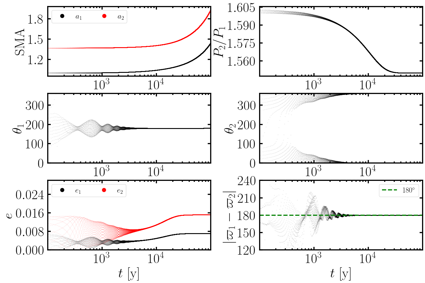
Figure 1: Standard MMR capture process for $h=0.03$ and $q=m_{1}/m_{2}=2$. The inner planet starts at the SMA $a_{1}=1$ au and the outer planet starts wide of the 2:3 resonance at $P_{2}/P_{1}=1.6$. Both planets have very small initial eccentricities, $e_{1}=e_{2}=0.001$. Note that to have convergent migration, we adopt $T_{m,i}<0$ (i.e. both planets migrate outwards). The planets are captured into the resonance around $t=20,000$ yrs, indicated by the libration of $\theta_{1}\to 180^{\circ}$ and $\theta_{2}\to 0^{\circ}$ and the period ratio approaching the equilibrium value ($\simeq 1.55$). While in resonance, the eccentricities are driven to the equilibrium values, $e_{1}\approx 0.008$ and $e_{2}\approx 0.016$, and the periapses are anti-aligned.

For two planets on coplanar orbits near the $j:j+1$ MMR, the Hamiltonian can be approximated to order $\mathcal{O}(e^{2})$ as (Murray & Dermott, 2000)

$$H=H_{\rm kep}+H_{\rm res}+H_{\rm sec},$$ (7)

with the Keplerian, resonant, and secular terms given by

$$H_{\rm kep}= -\frac{GMm_{1}}{2a_{1}}-\frac{GMm_{2}}{2a_{2}},$$ (8)

$$H_{\rm res}= -\frac{Gm_{1}m_{2}}{a_{2}}\left[f_{1}e_{1}\cos\theta_{1}+f_{2}e_{2}\cos\theta_{2}\right],$$ (9)

$$H_{\rm sec}= -\frac{Gm_{1}m_{2}}{a_{2}}\left[f_{3}(e_{1}^{2}+e_{2}^{2})+f_{4}e_{1}e_{2}\cos(\varpi_{2}-\varpi_{1})\right],$$ (10)

where $\theta_{1}$ and $\theta_{2}$ are given in equations (1) and (2). Here, the $f_{i}$ are functions of the semimajor axis ratio $\alpha=a_{1}/a_{2}$ that can be found in Appendix B of Murray & Dermott (2000):

$$f_{1} =\frac{1}{2}[2(j+1)+\alpha D]b_{1/2}^{(j+1)}(\alpha),$$ (11)

$$f_{2} =-\frac{1}{2}[2j+1+\alpha D]b_{1/2}^{(j)}(\alpha),$$ (12)

$$f_{3} =\frac{1}{8}[2\alpha D+\alpha^{2}D^{2}]b_{1/2}^{(0)}(\alpha),$$ (13)

$$f_{4} =\frac{1}{4}[2-2\alpha D-\alpha^{2}D^{2}]b_{1/2}^{(1)}(\alpha),$$ (14)

where $D\equiv d/d\alpha$ and the $b_{l}^{m}$ are Laplace coefficients. Near the 2:3 MMR, we have $f_{1}\approx 2.0$, $f_{2}\approx-2.5$, $f_{3}\approx 1.15$ and $f_{4}\approx 2.0$.

The Hamiltonian system defined by equation (7) admits eight coupled ordinary differential equations, which we may integrate together with dissipative terms (equations 3 and 4) to simulate MMR capture. The canonical Poincairé momentum-coordinate variables are

$$\Lambda_{i}=m_{i}\sqrt{GMa_{i}}, \quad\lambda_{i};$$ (15)

$$\Gamma_{i}=\Lambda_{i}(1-\sqrt{1-e_{i}^{2}})\simeq\frac{1}{2}\Lambda_{i}e_{i}^{2}, \quad-\varpi_{i}.$$ (16)

We apply Hamilton’s equations to generate the equations of motion (to second order in eccentricities) and add in the dissipative effects:

$$\frac{\dot{a}_{1}}{a_{1}} =\frac{2jn_{2}}{\sqrt{\alpha}}(f_{1}e_{1}\sin\theta_{1}+f_{2}e_{2}\sin\theta_{2})-\frac{1}{T_{m,1}}-\frac{e_{1}^{2}}{T_{e,1}},$$ (17)

$$\frac{\dot{a}_{2}}{a_{2}} =-2(j+1)\mu_{1}n_{2}(f_{1}e_{1}\sin\theta_{1}+f_{2}e_{2}\sin\theta_{2})-\frac{1}{T_{m,2}}-\frac{e_{2}^{2}}{T_{e,2}},$$ (18)

$$\dot{e}_{1} =-\frac{\mu_{2}n_{2}f_{1}}{\sqrt{\alpha}}\sin\theta_{1}+\frac{\mu_{2}f_{4}e_{2}n_{2}}{\sqrt{\alpha}}\sin(\varpi_{1}-\varpi_{2})-\frac{e_{1}}{T_{e,1}},$$ (19)

$$\dot{e}_{2} =-\mu_{1}n_{2}f_{2}\sin\theta_{2}-\mu_{1}f_{4}e_{1}n_{2}\sin(\varpi_{1}-\varpi_{2})-\frac{e_{2}}{T_{e,2}},$$ (20)

$$\dot{\lambda}_{1} =n_{1}+\frac{\mu_{2}n_{2}}{2\sqrt{\alpha}}f_{1}e_{1}\cos\theta_{1}$$

$$+\frac{\mu_{2}n_{2}}{\sqrt{\alpha}}\left(f_{3}e_{1}^{2}+\frac{f_{4}e_{1}e_{2}}{2}\cos(\varpi_{2}-\varpi_{1})\right),$$ (21)

$$\dot{\lambda}_{2} =n_{2}+\mu_{1}n_{2}\left(2f_{1}e_{1}\cos\theta_{1}+\frac{5}{2}f_{2}e_{2}\cos\theta_{2}\right)$$

$$+\mu_{1}n_{2}\left(2f_{3}e_{1}^{2}+3f_{3}e_{2}^{2}+\frac{5}{2}f_{4}e_{1}e_{2}\cos(\varpi_{2}-\varpi_{1})\right),$$ (22)

$$\dot{\varpi}_{1} =\frac{\mu_{2}n_{2}}{\sqrt{\alpha}e_{1}}f_{1}\cos\theta_{1}+\frac{\mu_{2}n_{2}}{\sqrt{\alpha}}\left(2f_{3}+f_{4}\frac{e_{2}}{e_{1}}\right),$$ (23)

$$\dot{\varpi}_{2} =\frac{\mu_{1}n_{2}}{e_{2}}f_{2}\cos\theta_{2}+\mu_{1}n_{2}\left(2f_{3}+f_{4}\frac{e_{1}}{e_{2}}\right).$$ (24)

Note that the right-hand sides of these equations depend on $\lambda_{1}$ and $\lambda_{2}$ solely through the combination $(j+1)\lambda_{2}-j\lambda_{1}$. By combining equations (2.1) and (2.1) into a single equation for $(j+1)\dot{\lambda}_{2}-j\dot{\lambda}_{1}$, we may reduce the number of equations to seven. We integrate the system with the Runge-Kutta method of order 5(4) included in the $\mathtt{scipy}$ Python package. We set a relative and absolute tolerance $\epsilon=10^{-9}$. The resonance angles are initialized over a uniform distribution between $0^{\circ}$ and $360^{\circ}$. At $t=0$, we set $a_{1}=1~{}\mathrm{au}$, $P_{2}/P_{1}=1.6$, and $e_{1}=e_{2}=0.001$.

An example of MMR capture is shown in Fig. 1. The period ratio $P_{2}/P_{1}$ starts wide of the nominal 2:3 resonance value. After around $2~{}\rm{kyr}$ of convergent migration, the planets are caught into the MMR, indicated by the stabilization of $\theta_{1}$ to $180^{\circ}$ and $\theta_{2}$ to $0^{\circ}$. The planets’ eccentricities level off at their equilibrium values at $e_{1}\approx 0.008$ and $e_{2}\approx 0.016$, and the planets become apsidally anti-aligned with $\varpi_{1}-\varpi_{2}\approx 180^{\circ}$.

The final period ratio $P_{2}/P_{1}\simeq 1.55$ differs from 3/2, which can be explained by the equations for $\dot{\theta}_{1}=(j+1)\dot{\lambda}_{2}-j\dot{\lambda}_{1}-\dot{\varpi}_{1}$ and $\dot{\theta}_{2}=(j+1)\dot{\lambda}_{2}-j\dot{\lambda}_{1}-\dot{\varpi}_{2}$. If we truncate the equations to lowest order in eccentricity ($\mathcal{O}(e_{i}^{-1})$), the dynamics are dominated by the $\dot{\varpi}_{i}$ terms (equations 23 and 24), and we have

$$\dot{\theta}_{1} \simeq(j+1)n_{2}-jn_{1}-\frac{\mu_{2}n_{2}}{\sqrt{\alpha}e_{1}}|f_{1}|\cos\theta_{1},$$ (25)

$$\dot{\theta}_{2} \simeq(j+1)n_{2}-jn_{1}+\frac{\mu_{1}n_{2}}{e_{2}}|f_{2}|\cos\theta_{2}.$$ (26)

Hence, in equilibrium, it is expected that $P_{2}/P_{1}=n_{1}/n_{2}>(j+1)/j=1.5$ for the observed values of $\theta_{1}=180^{\circ}$ and $\theta_{2}=0^{\circ}$.

2.2 Equilibrium

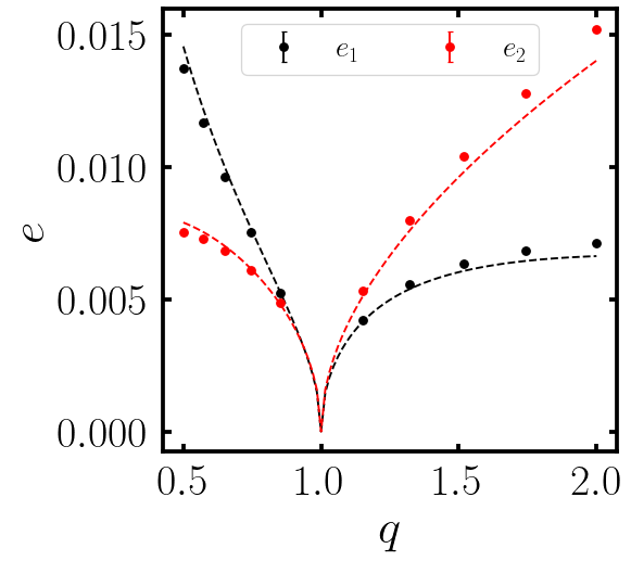
(a)

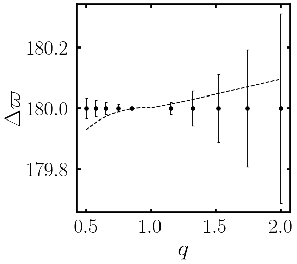
(b)

Figure 2: Equilibrium eccentricities $e_{1},e_{2}$ (left) and relative apsidal angle $\Delta\varpi=\varpi_{1}-\varpi_{2}$ (right) for two planets captured into the 2:3 MMR, plotted against the mass ratio $q=m_{1}/m_{2}$. The dashed lines are analytical results determined by solving equations (27) – (2.2) and (2.2). The dots are obtained by integrating the time-dependent equations of motion and time-averaging the eccentricities over the last 10% of the integration. We hold $h=0.03$ and $T_{e,0}=\sqrt{T_{e,1}T_{e,2}}=1000$ yrs constant, but allow the eccentricity damping and migration timescales to vary with $q$, as in equations (5) and (6).

The MMR capture shown in Fig. 1 leads to an equilibrium state in period ratio, resonant angles, eccentricities, and $\Delta\varpi$. By requiring $\dot{e}_{1}=0$, $\dot{e}_{2}=0$, and $\dot{\varpi}_{1}-\dot{\varpi}_{2}=0$, we arrive at three equations:

$$\dot{e}_{1}=-\frac{\mu_{2}n_{2}}{\sqrt{\alpha}}[f_{1}\sin\theta_{1}-f_{4}e_{2}\sin(\varpi_{1}-\varpi_{2})]-\frac{e_{1}}{T_{e,1}}=0$$ (27)

$$\dot{e}_{2}=-q\mu_{2}n_{2}[f_{2}\sin\theta_{2}+f_{4}e_{1}\sin(\varpi_{1}-\varpi_{2})]-\frac{e_{2}}{T_{e,2}}=0$$ (28)

$$\frac{d}{dt}\Delta\varpi=\dot{\varpi}_{1}-\dot{\varpi}_{2} =\mu_{2}n_{2}\left[\frac{f_{1}\cos\theta_{1}}{\sqrt{\alpha}e_{1}}-\frac{qf_{2}\cos\theta_{2}}{e_{2}}\right.$$

$$\quad+\left.\frac{2f_{3}}{\sqrt{\alpha}}+\frac{f_{4}e_{2}}{\sqrt{\alpha}e_{1}}-2qf_{3}-\frac{qf_{4}e_{1}}{e_{2}}\right]=0.$$ (29)

To first order in eccentricity, the first two equations determine the equilibrium values of $\theta_{1}$ and $\theta_{2}$, while the last implies that $e_{2}/e_{1}\sim q=m_{1}/m_{2}$. In the absence of dissipation, the following quantities are strictly conserved (e.g. Xu et al., 2018):

$$J =\Lambda_{1}\sqrt{1-e_{1}^{2}}+\Lambda_{2}\sqrt{1-e_{2}^{2}},$$ (30)

$$K =\frac{j+1}{j}\Lambda_{1}+\Lambda_{2}.$$ (31)

Following Xu et al. (2018), we define

$$\eta(\alpha,e_{1},e_{2}) \equiv-2(q/\alpha_{0}+1)\left(\frac{J}{K}-\left.\frac{J}{K}\right|_{0}\right),$$ (32)

where $\alpha_{0}=[j/(j+1)]^{2/3}$ and $\left.(J/K)\right|_{0}$ is evaluated at $e_{i}=0$ and $\alpha=\alpha_{0}$. For $|\alpha-\alpha_{0}|\ll 1$ and $e_{1},e_{2}\ll 1$, we have

$$\eta\simeq\frac{q(\alpha-\alpha_{0})}{j\sqrt{\alpha_{0}}(q/\alpha_{0}+1)}+q\sqrt{\alpha_{0}}e_{1}^{2}+e_{2}^{2}.$$ (33)

Since $\eta$ is conserved in the absence of dissipation, the only nonzero terms in its derivative, $\dot{\eta}$, can be from the dissipative effects. In equilibrium, we require $\dot{\eta}=0$, i.e.

$$\dot{\eta}=\frac{q\alpha}{j\sqrt{\alpha_{0}}(q\alpha_{0}^{-1}+1)} \left[\frac{1}{T_{m,2}}-\frac{1}{T_{m,1}}+\frac{2e_{1}^{2}}{T_{e,1}}-\frac{2e_{2}^{2}}{T_{e,2}}\right]$$

$$-q\alpha_{0}^{1/2}\frac{2e_{1}^{2}}{T_{e,1}}-\frac{2e_{2}^{2}}{T_{e,2}}=0.$$ (34)

We note that $\dot{\eta}$ depends only on the effective migration rate, $1/T_{m}\equiv 1/T_{m,2}-1/T_{m,1}$.

Utilizing the $\mathtt{scipy}$ root finding library, assuming $\alpha=\alpha_{0}$, we solve the four equations (27) – (2.2) and (2.2) for the equilibrium values of $\theta_{1},\theta_{2},e_{1},e_{2}$. The equilibrium $e_{i}$’s and $\Delta\varpi$’s for comparable mass planets $(q\in[0.5,2])$ are given in Figures 2(a) and 2(b) as the dashed lines. The equilibrium eccentricities go approximately as $e_{2}/e_{1}\sim q$, and all systems are predicted to have $\Delta\varpi\approx 180^{\circ}$. To validate these analytical results, we also integrate the time dependent equations which simulate MMR capture and plot the average $e_{1}$, $e_{2}$, and $\Delta\varpi$ over the last 10% of the simulation. For $T_{e,1}<T_{e,2}$ ($T_{e,1}>T_{e,2}$), we set $T_{m,i}<0$ ($T_{m,i}>0$), corresponding to outward (inward) migration. The numerical (markers) and analytical (dashed lines) results largely agree. Thus, in the standard picture of MMR capture in PPDs, comparable mass planets always end up settling down to $\theta_{1}\approx 180^{\circ}$ and $\theta_{2}\approx 0^{\circ}$, and the eccentricity vectors of the planets are anti-aligned, $|\Delta\varpi|=|\varpi_{1}-\varpi_{2}|=|\theta_{2}-\theta_{1}|=180^{\circ}$.

2.3 Survey of parameter space: Eccentricity damping timescales

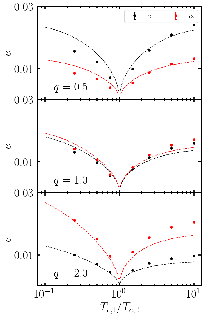
Figure 3: The final time-averaged eccentricities (dots) of the two planets captured in the 2:3 MMR as a function of $T_{e,1}/T_{e,2}$ for $q=m_{1}/m_{2}=0.5,1,$ and $2$. We have kept $T_{e,0}$, $h$ and the initial conditions fixed to the same values as in Figure 1. The dashed lines indicate the analytical equilibrium eccentricities obtained by solving equations (27) – (2.2) and (2.2), as in Fig. 2(a). For $T_{e,1}/T_{e,2}>1$ ($T_{e,1}/T_{e,2}<1$), migration is inward (outward), since we keep the ratio $T_{e,i}/|T_{m,i}|\propto h^{2}$. For $q=0.5$, the inward migrating branch ($T_{e,1}>T_{e,2}$) agrees well with the equilibrium result. However, for the outward migrating branch the analytic solution typically overestimates the final eccentricities. The results are similar for $q=1,2$.

Figure 4: Same as Fig. 3 but showing $\Delta\varpi$. In all cases the apsides of the two planets are anti-aligned.

In Section 2.2, we adopted the standard scaling relation – with $T_{e,1}/T_{e,2}=1/q=m_{2}/m_{1}$ and $T_{e,i}=3.46h^{2}|T_{m,i}|$ – which always gives rise to apsidal anti-alignment for typical disc conditions ($h\lesssim 0.1$) and planet masses. A real PPD may have significant surface density variation that leads to a different ratio $T_{e,1}/T_{e,2}$. Here we study the effects of different $T_{e,1}/T_{e,2}$ on the equilibrium values of $e_{i}$ and whether such a change could lead to apsidal alignment.

We explore this possibility in Figures 3 and 4 by varying $T_{e,1}/T_{e,2}$ between $0.2$ and $10$, regardless of the mass ratio. The migration timescale is still set to $|T_{m,i}|=T_{e,i}/(3.46h^{2})$. We can see that for comparable mass planets with $q=0.5$, $1$, and $2$, varying the ratio $T_{e,1}/T_{e,2}$ around $1/q$ modifies the final equilibrium eccentricities by a roughly similar factor. The dashed lines of Fig. 3 show the analytic results from solving equations (27) – (2.2) and (2.2); these results agree with our time dependent integrations.

For integrations where the migration direction is the opposite of what it would be if $T_{e,1}/T_{e,2}=1/q=m_{2}/m_{1}$ (i.e., $T_{e,1}/T_{e,2}<1$ for $q=0.5$), the analytical results systematically overestimate the final eccentricities for $T_{e,1}/T_{e,2}<1$, and underestimate them for $T_{e,1}/T_{e,2}>1$. The eccentricity ratio $e_{1}/e_{2}$ is unchanged, yet $e_{1}$ and $e_{2}$ are larger for more extreme values of $T_{e,1}/T_{e,2}$. The corresponding values for $\Delta\varpi$ are shown in Fig. 4. In all cases, both the analytic equilibrium equations and the numerical integrations yield $\Delta\varpi\simeq 180^{\circ}$.

The peaked shape of the dashed lines in Figures 2(a) and 3 can be explained as follows. As $T_{m,1}/T_{m,2}=T_{e,1}/T_{e,2}$ approaches unity, the effective migration timescale $T_{m}$ approaches infinity. Equation (2.2) therefore implies that the planets’ eccentricities approach zero. We note that the equilibrium solutions are not continuous across $q=1$ (Fig. 2) and $T_{e,1}/T_{e,2}=1$ (Figures 3 and 4), which is where we reverse the migration direction to ensure that it is convergent.

In summary, we find that varying the eccentricity damping ratio cannot account for the observed apsidal alignment in some MMR systems (such as K2-19). Before proposing a possible solution in Section 4, we consider in Section 3 the simpler problem of a test mass orbiting near a MMR with a finite-mass planet in order to gain some insight on the dynamics of apsidal angles.

3 MMR in the Restricted 3-body Problem

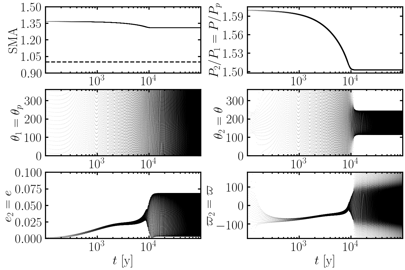
Figure 5: The capture process of a test particle into the 2:3 MMR with a massive planet with $\mu_{p}=10^{-4}$, $a_{p}=1$ au and eccentricity $e_{p}=0.04$. We have set $h=0.03$ (which gives $e_{\rm eq}=0.028$) and $T_{e}=1000P_{p}$. After the particle is captured into resonance, both $\theta_{2}$ and $e$ librate with large amplitude, and $\varpi$ circulates.

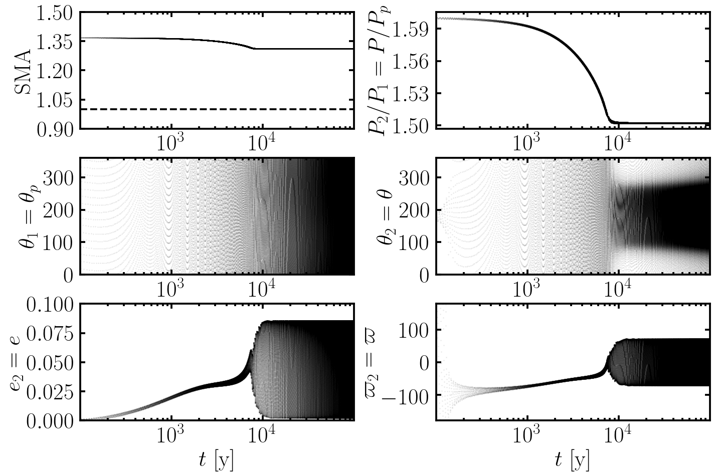
Figure 6: Same as Fig. 5, except $e_{p}=0.054$. Although $P_{2}/P_{1}$ settles down to a value very close to 3/2, the resonance angle $\theta_{2}$ circulates throughout the evolution. As in Fig. 5, the test particle eccentricity librates with large amplitude, but now its apsidal angle becomes aligned with $\varpi_{p}\equiv 0^{\circ}$.

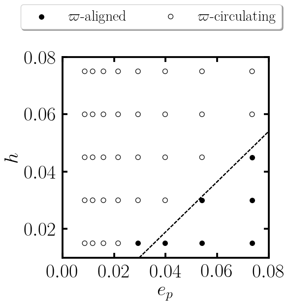
Figure 7: The behavior of the final $\Delta\varpi$ for a range of values for $h$ and $e_{p}$ when an exterior test mass is captured into the 2:3 MMR with a planet of mass $\mu_{p}=10^{-4}$. For a given $h$, the system becomes apsidally aligned for sufficiently large $e_{p}$ (see Fig. 6 for an example). The dashed line indicates our analytical approximation for the boundary between the $\varpi$-aligned and $\varpi$-circulating regions.

The dynamics of first-order MMRs with comparable mass planets is complicated by the presence of two critical arguments in the Hamiltonian, $\theta_{1}$ and $\theta_{2}$. By assuming that one of the planets is a test particle, we may ignore the dynamical evolution of the other planet. To emphasize the fact that we are formally transitioning to a different problem, we adopt the following notation: The subscript $p$ will denote the quantities associated with the massive planet, while no subscript will indicate those associated with the test particle. Neglecting additive constants, the Hamiltonian for an exterior test particle ($m_{2}=0$) is given by

$$H= -\frac{GM}{2a}-\frac{Gm_{p}}{a_{p}}[f_{1}e_{p}\cos\theta_{p}+f_{2}e\cos\theta$$

$$+f_{3}e^{2}+f_{4}ee_{p}\cos(\varpi_{1}-\varpi_{2})].$$ (35)

We assume that no dissipative force acts on the massive planet while implementing the same force as in Section 2 for the test particle.

3.1 Circular massive planet: $e_{p}=0$

When a test particle is caught into a stable resonance, its eccentricity grows and saturates at a finite value which depends on the ratio $T_{e}/T_{m}$ (e.g. Goldreich & Schlichting, 2014; Xu et al., 2018). For an exterior test particle,

$$e_{\rm eq}=\sqrt{\frac{T_{e}}{2jT_{m}}}=h\sqrt{\frac{1.73}{j}}.$$ (36)

If $e_{p}=0$, the system has no preferred direction, and so $\varpi$ must circulate.

3.2 Eccentric massive planet

When the massive planet has a moderate eccentricity, the qualitative features of the $e_{p}=0$ result are preserved as long as $e_{p}\lesssim e_{\rm eq}$. In Fig. 5, we show the capture process for a system with $e_{p}=0.04$ and $h=0.03$ (thus $e_{\rm eq}=0.028$). As we can see, the particle is still captured into the 2:3 resonance and $\theta_{2}$ librates around 180^∘. The eccentricity $e$ librates around its equilibrium value with large amplitude, and the longitude of perihelion, $\varpi$, still circulates.

Fig. 6 shows the capture process for $e_{p}=0.054$ (and the same $e_{\rm eq}=0.028$). We see that, for $e_{p}\gtrsim e_{\rm eq}$, the test particle’s migration halts near the nominal resonance location of $P_{2}/P_{1}=1.5$ while both $\theta_{1}$ and $\theta_{2}$ continue to circulate. The particle’s eccentricity librates with slightly larger amplitude than in Fig. 5. Eventually, the system becomes apsidally aligned.

In Fig. 7, we summarize the behavior of the final $\Delta\varpi$ for an exterior test particle captured into the 2:3 MMR with a massive planet, for different values of $e_{p}$ and $h$ (and subsequently $e_{\rm eq}$). Generally, for $e_{p}\gtrsim e_{\rm eq}$, the system becomes apsidally aligned.

4 Eccentricity Driving by Disc and Apsidal Alignment in MMR

We have seen in Section 2 that whenever two comparable-mass planets are captured into the $\theta_{1}$ and $\theta_{2}$ resonances, the system always has $\Delta\varpi\approx 180^{\circ}$ because $\theta_{1}$ and $\theta_{2}$ settle down to $180^{\circ}$ and $0^{\circ}$, respectively. The apsidally aligned K2-19 system (see Section 1) therefore poses a problem for the standard migration-driven MMR capture model. In order to match this observation, either $\theta_{1}$, $\theta_{2}$, or both angles must circulate.

In Section 3, we have seen that apsidal alignment arises whenever the massive planet has an eccentricity larger than the equilibrium eccentricity of the test particle in resonance. Guided by this result, in this section, we examine the possibility that planet-disc interaction drives planet’s eccentricity to a finite value and explore its consequences for the apsidal angles in MMR capture. In addition, we reformulate the 2-planet Hamiltonian into a single-degree of freedom system; this allows us to identify the key dynamical processes that lead to apsidal alignment.

4.1 Effects of disc eccentricity driving on MMR

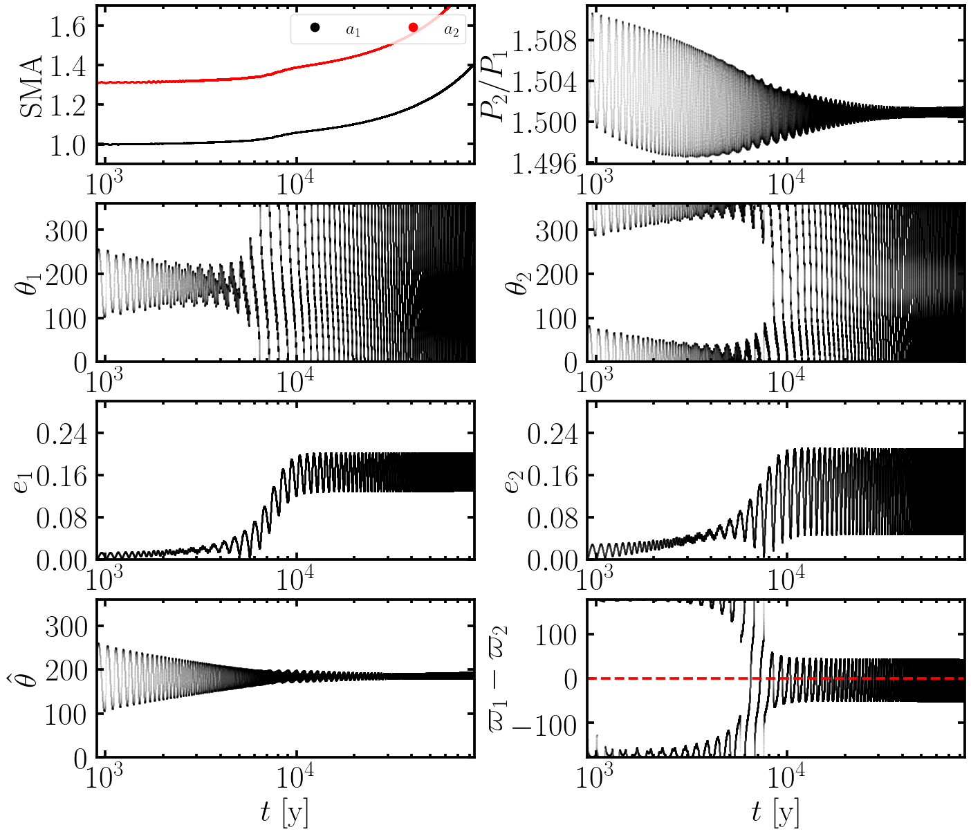
Figure 8: Capture of comparable mass ($q=m_{1}/m_{2}=2$) planets into the 3:2 MMR with $e_{1,d}=0.2$, $e_{2,d}=0$ (see equation 37)and $h=0.03$. All other initial conditions are the same as in Fig. 1, except for the initial period ratio, which we set to the nominal resonance location, $P_{2}/P_{1}=1.5$, so that the system is very quickly caught into the $\theta_{1}$ and $\theta_{2}$ resonances. After about 10 kyr, the system escapes the circular resonances, indicated by the circulation of $\theta_{1}$ and $\theta_{2}$. At this point, the planets becomes apsidally aligned and $\Delta\varpi$ librates around $0^{\circ}$.

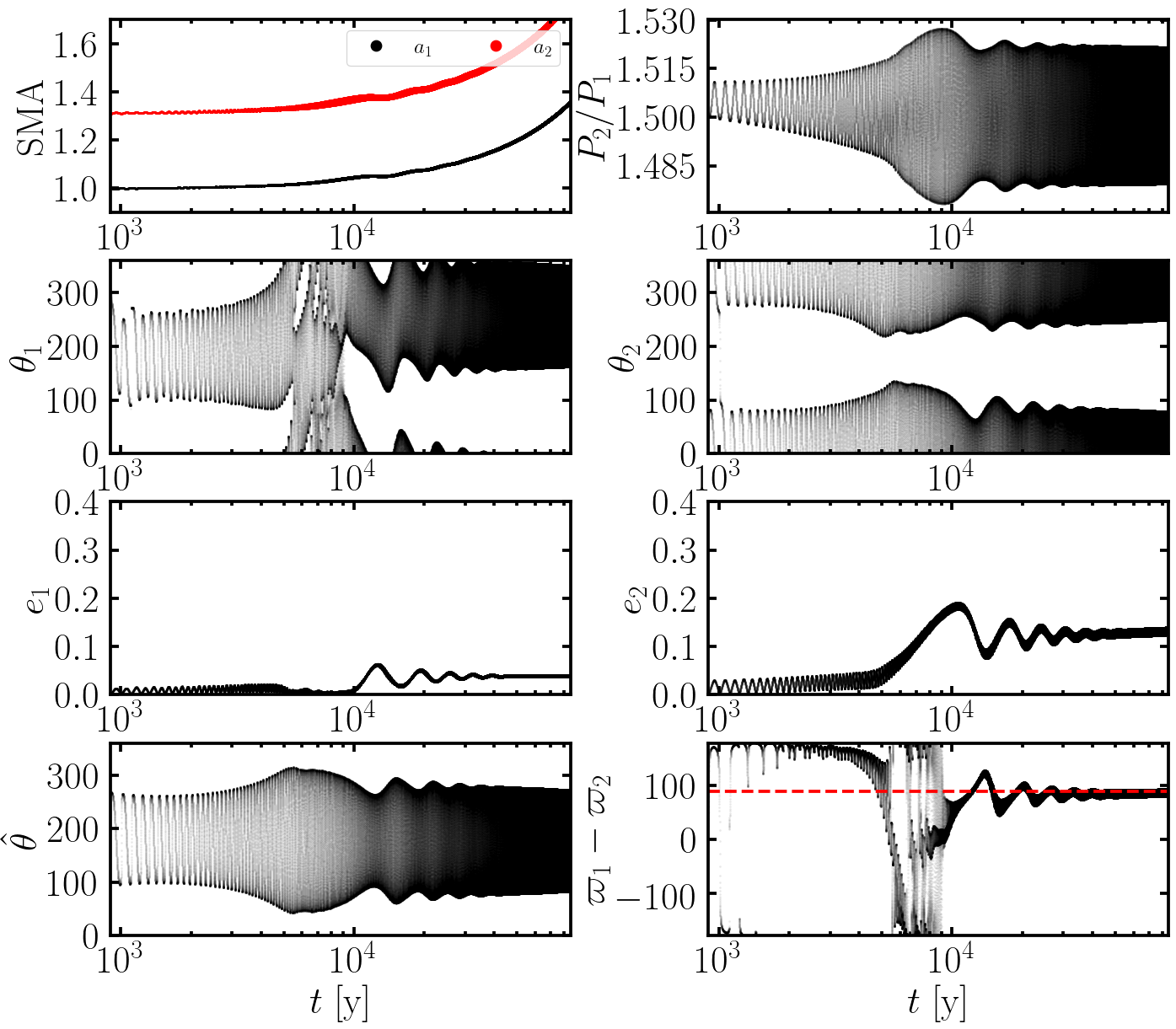
Figure 9: Same as Fig. 8, but with $e_{1,d}=0$ and $e_{2,d}=0.2$. After about 10 kyr, the system escapes the $\theta_{1}$ resonance, indicated by its shift in libration center to $270^{\circ}$ rather than $180^{\circ}$. We see that $\theta_{2}$ still librates around $0^{\circ}$, and so the apsidal angles of the planets reach $\Delta\varpi=90^{\circ}$.

As noted in Section 1, under appropriate conditions, planet-disc interactions can increase a planet’s eccentricity rather than damp it (e.g. Goldreich & Sari, 2003; Teyssandier & Ogilvie, 2017; Ragusa et al., 2017). A recent study demonstrates that a super-earth-sized luminous protoplanet can attain an eccentricity larger than the disc aspect ratio (Romero et al., 2021).

The planets K2-19b and c are moderately eccentric, with $e_{b}\approx e_{c}\approx 0.2$ (Petigura et al., 2020). Petit et al. (2020) suggest that the apsidal alignment in this system could be caused by eccentricity driving to a common value. To mimic the effect of eccentricity driving by the disk, we modify the eccentricity damping term in equation (4) to

$$\frac{\dot{e}_{i}}{e_{i}}=-\frac{(e_{i}-e_{i,d})}{T_{e,i}},$$ (37)

so that planet $m_{i}$ is driven toward $e_{i,d}$ on the timescale $T_{e,i}$.

In Fig. 8, we show the result of MMR capture for a system with $e_{1,d}=0.2$, $e_{2,d}=0.0$, and mass ratio $q=m_{1}/m_{2}=2$. We initialize the system with $e_{1}=e_{2}=0.001$ at the nominal resonance location, $P_{2}/P_{1}=1.5$. The planets are caught in the $\theta_{1}$ and $\theta_{2}$ resonances for 10,000 years, after which the planets escape the resonance and the angles circulate. At this point, both planets’ eccentricities are excited to about $e_{i}\approx 0.2$ and the planets become apsidally aligned as $\Delta\varpi$ librates around $0^{\circ}$ with a large amplitude. Despite the circulation of both resonance angles, the period ratio remains locked very close to the nominal resonance value ($P_{2}/P_{1}=1.5$). The system is caught in a different type of resonance which we will study in the following subsection.

On the other hand, for $e_{2,d}=0.2$ and $e_{1,d}=0$, the system displays different resonance capture behavior. We show the result for this case in Fig. 9. We see that the angle $\theta_{2}$ librates with a large amplitude around its resonant value of $0^{\circ}$, whereas $\theta_{1}$ librates around $270^{\circ}$ rather than $180^{\circ}$. As a result, $\Delta\varpi$ approaches $90^{\circ}$, i.e. the planets’ perihelia are now perpendicular to each other.

4.2 Reducing the Hamiltonian

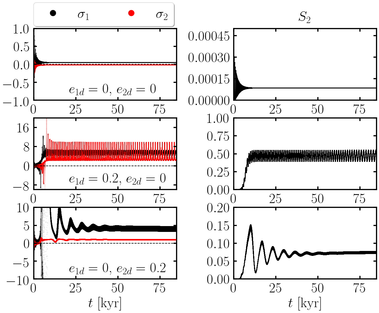
Figure 10: The quantities $\sigma_{1}$ and $\sigma_{2}$ (left) and the quantity $S_{2}$ (right, see equations 40, 42 and 43) for the three different combinations of $e_{1d}$ and $e_{2d}$ corresponding to the systems depicted in Figures 1, 8, and 9. Each row corresponds to one of the three different modes of resonance identified in this paper, $\Delta\varpi=180^{\circ}$, $\Delta\varpi=0^{\circ}$, and $\Delta\varpi=90^{\circ}$, respectively. For $\Delta\varpi=180^{\circ}$ (upper row), $\sigma_{1}$, $\sigma_{2}$, and $S_{2}$ are conserved near zero. For the other two cases, $S_{2}$ transitions to larger values near $\sim 0.5$ (middle) and $\sim 0.1$ (bottom) as the eccentricity reaches an equilibrium. Both $\sigma_{1}$ and $\sigma_{2}$ are excited to factors of a few in the apsidally aligned case (middle row), while only $\sigma_{1}$ is excited for the $\Delta\varpi=90^{\circ}$ case (bottom row). For $\Delta\varpi=0^{\circ}$ and $\Delta\varpi=90^{\circ}$ cases, the eccentricities oscillate in such a way to conserve $S_{2}$ according to equation (41).

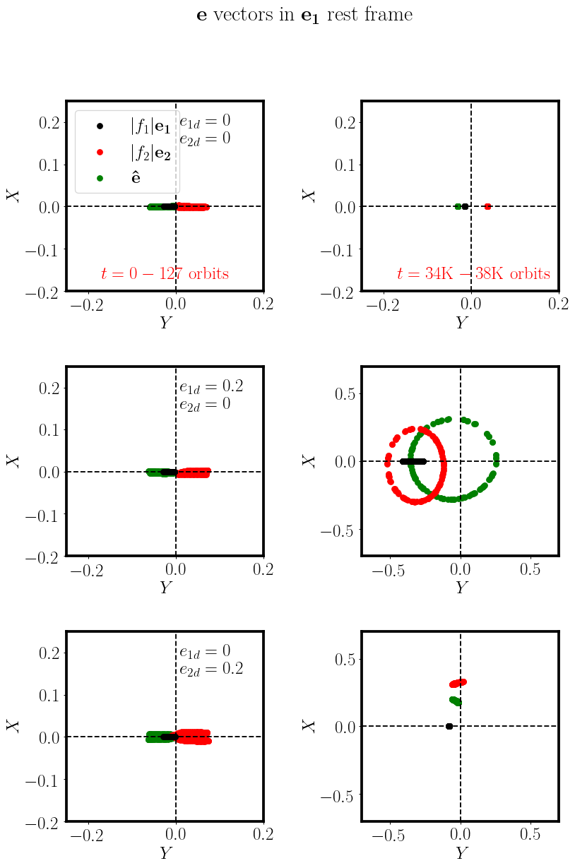
Figure 11: The eccentricity vectors $\mathbf{e}_{1}$, $\mathbf{e}_{2}$, and $\mathbf{\hat{e}}$ in the reference frame rotating with $\mathbf{e}_{1}$. As in Fig. 10, each row represents the different combination of $e_{1d}$ and $e_{2d}$ corresponding to the three different modes of resonance. The left column shows the initial conditions of the resonance, while the right column shows the evolution at late times (at $t=[34-38]\times 10^{3}$ orbits). The top row ($\Delta\varpi=180^{\circ}$) exhibits little qualitative change between the initial and late times besides the libration amplitudes shrinking to zero. The second row ($\Delta\varpi=0^{\circ}$) shows $\mathbf{e}_{2}$ circulating around $\mathbf{e}_{1}$ strictly contained to the second and third quadrants. The last row ($\Delta\varpi=90^{\circ}$) shows $\mathbf{e}_{1}$ and $\mathbf{e}_{2}$ transitioning into a perpendicular arrangement. Meanwhile, the $\mathbf{\hat{e}}$ vector circulates outside of both $\mathbf{e}_{1}$ and $\mathbf{e}_{2}$ in the second row, while remaining aligned with $\mathbf{e}_{2}$ in the bottom row.

To understand the results of Section 4.1, we carry out an analysis of the MMR Hamiltonian (equation 7). This helps to illustrate the underlying dynamics behind the capture process in Fig. 8 which leads to apsidal alignment. It can be shown that $\theta_{1}$ and $\theta_{2}$ are actually subresonances of a resonance $\hat{\theta}$, which arises after transforming the system’s Hamiltonian so that it has only a single degree of freedom (Henrard et al., 1986; Deck et al., 2013).

If we assume that the secular behavior of the semi-major axis ratio $\alpha$ is stationary or varying adiabatically, we may transform the resonant Hamiltonian $H_{\rm Kep}+H_{\rm res}$ in equation (7) into the form

$$\hat{H}(\hat{R},\hat{\theta})=-3(\delta+1)\hat{R}+\hat{R}^{2}-2\sqrt{2\hat{R}}\cos\hat{\theta}$$ (38)

through a series of rotations in phase space. For the details of these transformations, see Appendix A. The Hamiltonian in equation (38) is well studied in the literature (e.g., Murray & Dermott, 2000). The parameter $\delta$ quantifies the system’s depth into resonance. We do not include $H_{\rm sec}$ in this analysis because it is second order in eccentricities.

In equation (38), the action $\hat{R}$ is a function of both $e_{1}$ and $e_{2}$. Define $\boldsymbol{\hat{e}}=|f_{1}|\boldsymbol{e}_{1}-|f_{2}|\boldsymbol{e}_{2}$ and $\hat{e}=|\boldsymbol{\hat{e}}|$, where $\boldsymbol{e}_{i}$ is the eccentricity (Runge-Lenz) vector of each planet. The action $\hat{R}$ takes the form $\hat{R}\propto\tilde{\mu}\hat{e}^{2}$, where $\tilde{\mu}=\tilde{m}/M$ and $\tilde{m}=m_{1}m_{2}/(m_{1}+m_{2})$. The coordinate angle, $\hat{\theta}$, is given by

$$\tan\hat{\theta}=\frac{f_{1}e_{1}\sin\theta_{1}+f_{2}e_{2}\sin\theta_{2}}{f_{1}e_{1}\cos\theta_{1}+f_{2}e_{2}\cos\theta_{2}}.$$ (39)

This angle is the same one that Petit et al. (2020) found to librate in the K2-19 system.

4.3 Three modes of resonance

The one-degree-of-freedom Hamiltonian (equation 38) admits the following conserved quantity:

$$S_{2}=q\sqrt{\alpha}f_{2}^{2}e_{1}^{2}+2|f_{1}f_{2}|e_{1}e_{2}\cos(\varpi_{1}-\varpi_{2})+\frac{f_{1}^{2}}{q\sqrt{\alpha}}e_{2}^{2}.$$ (40)

By enforcing $dS_{2}/dt=0$ together with the assumption $d\alpha/dt=0$, we arrive at the following equilibrium condition:

$$\frac{dS_{2}}{dt}\propto e_{1}^{2}\left(\frac{e_{1}-e_{1\rm d}}{T_{e,1}}\right)\left|\frac{f_{2}}{f_{1}}\right|\sigma_{1}+e_{2}^{2}\left(\frac{e_{2}-e_{2\rm d}}{T_{e,2}}\right)\sigma_{2}=0,$$ (41)

where

$$\sigma_{1}= \left[q^{2}\alpha\left|\frac{f_{2}}{f_{1}}\right|+\frac{e_{2}}{e_{1}}q\sqrt{\alpha}\cos(\varpi_{1}-\varpi_{2})\right],$$ (42)

$$\sigma_{2}= \left[\left|\frac{f_{2}}{f_{1}}\right|q\sqrt{\alpha}\frac{e_{1}}{e_{2}}\cos(\varpi_{1}-\varpi_{2})+1\right].$$ (43)

The systems depicted in Figures 1, 8, and 9 are representative of three different modes of resonance, ones with $\Delta\varpi\simeq 180^{\circ}$, $\Delta\varpi\simeq 0^{\circ}$, and $\Delta\varpi\simeq 90^{\circ}$, respectively. These correspond to three different behaviors of the quantities $\sigma_{1}$ and $\sigma_{2}$ while in resonance under the influence of eccentricity forcing. In Fig. 10, we show $\sigma_{1}$, $\sigma_{2}$, and $S_{2}$ for these systems. The top row is for the standard eccentricity damping case where $e_{1d}=e_{2d}=0$. Once the system equilibrates, $S_{2}\approx 10^{-4}$ is well conserved (top left) and small. Both $\sigma_{1}$ and $\sigma_{2}$ are also close to zero. From equations (42) and (43), we see this corresponds to $e_{2}/e_{1}\sim q$, as we found in Section 2. The second row of Fig. 10 corresponds to the system shown in Fig. 8, where $e_{1d}=0.2$ and $e_{2d}=0$. At early times, while the system is still caught in the $\theta_{1}$ and $\theta_{2}$ resonances, $\sigma_{1}$, $\sigma_{2}$, and $S_{2}$ are small. Once the $\theta_{1}$ and $\theta_{2}$ resonances are broken, and only $\hat{\theta}$ librates, $\sigma_{1}$, $\sigma_{2}$ and $S_{2}$ are excited to larger values. The quantities $\sigma_{1}$ and $\sigma_{2}$ undergo large periodic oscillations away from zero, while $S_{2}$ grows and then stabilizes at its new equilibrium value, $S_{2}\approx 0.5$. The planets’ eccentricities oscillate in such a way as to conserve $S_{2}$. The bottom row of Fig. 10 corresponds to the system in Fig. 9, where $e_{2d}=0.2$ and $e_{1d}=0$, where the planets’ perihelia are perpendicular. For this case, $\sigma_{2}$ is conserved close to 0, while $\sigma_{1}$ grows to a magnitude similar to its value in the apsidally aligned case.

In Fig. 11, we plot the eccentricity vectors $\mathbf{e}_{1}$, $\mathbf{e}_{2}$, and $\mathbf{\hat{e}}$ in the reference frame rotating with $\mathbf{e}_{1}$. The three systems begin with the same configuration, caught in the $\theta_{1}$ and $\theta_{2}$ resonances; the vectors $\mathbf{e}_{1}$ and $\mathbf{e}_{2}$ are anti-aligned, while $\mathbf{\hat{e}}$ is aligned with $\mathbf{e}_{1}$. At later times, the system without eccentricity driving remains in this configuration (top row). The second and third rows exhibit the new resonance behaviors described above. For the apsidally aligned case (middle row), $\mathbf{e_{2}}$ circulates in a pattern strictly constrained to the second and third quadrants, and $\mathbf{\hat{e}}$ circulates around the other two vectors. In the bottom row, $\mathbf{e}_{1}$ and $\mathbf{e}_{2}$ are perpendicular to each other and $\mathbf{\hat{e}}$ is aligned with $\mathbf{e}_{2}$.

4.4 Dependence on $e_{\rm 1,d}$ and $e_{\rm 2,d}$

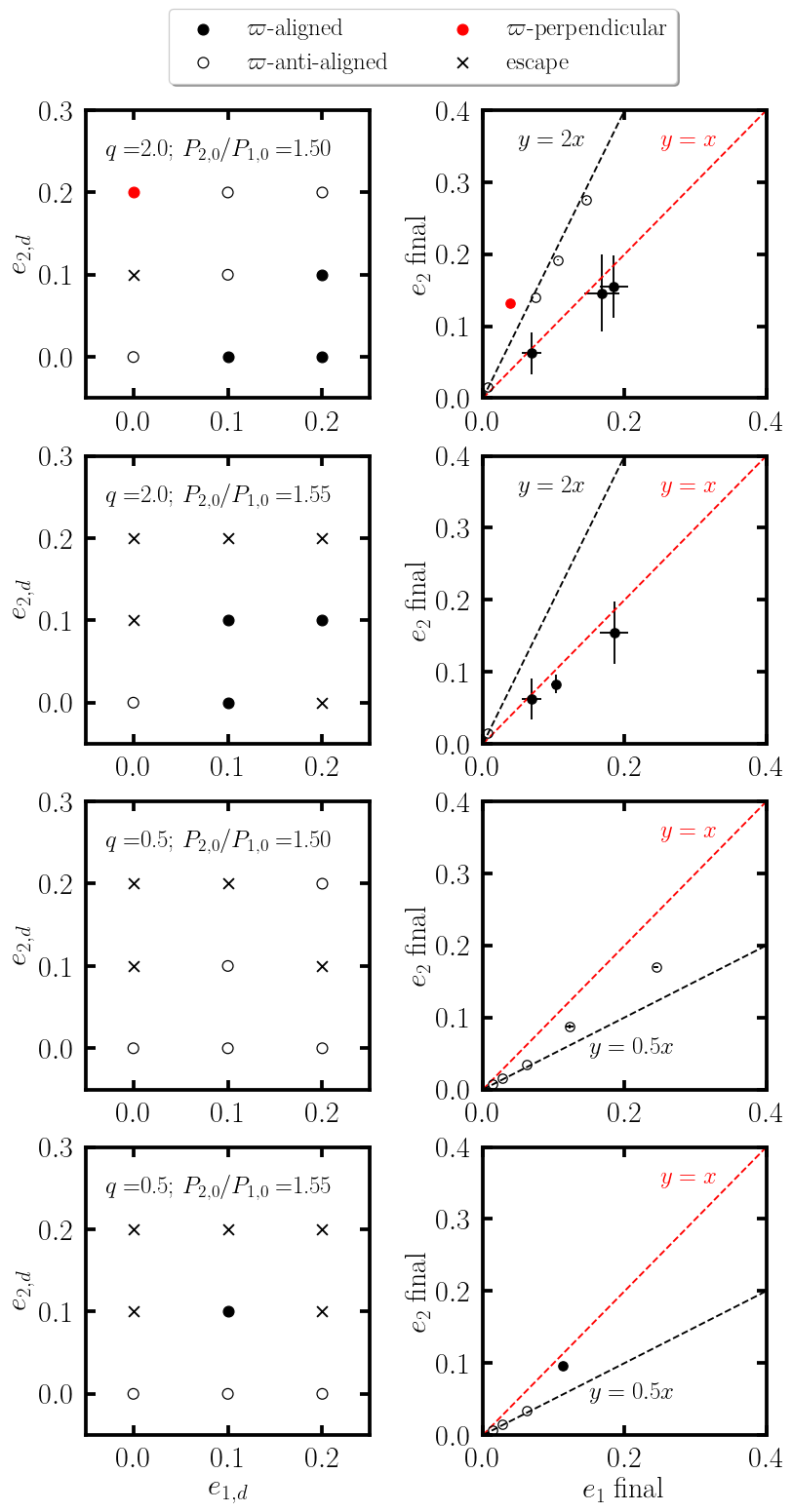
Figure 12: The resonance architecture for systems spanning a grid of driving eccentricities $e_{1,d},e_{2,d}$ (left) and the numerically averaged final eccentricities (right). We hold $h=0.03$ and $T_{e,0}=1000$ yrs, while varying $e_{1,d}$ and $e_{2,d}$. Systems which are not captured or become unstable and escape resonance are denoted by black “x”-marks. Roughly, for $e_{1d}\gtrsim e_{2d}$, the system becomes aligned. For $e_{2d}\gtrsim e_{1d}$, the system becomes perpendicular ($\Delta\varpi=90^{\circ}$) for large values of $e_{2d}$. The other systems remain trapped in both of the $\theta_{1}$ and $\theta_{2}$ resonances. The time-averaged eccentricities of the apsidally aligned systems fall just below the line $e_{2}=e_{1}$. The error bars are their standard deviations. The single perpendicular system (see the top left panel) falls just above the line $e_{2}=2e_{1}=qe_{1}$, while the anti-aligned systems fall just below it. Both have small librations compared to the aligned case.

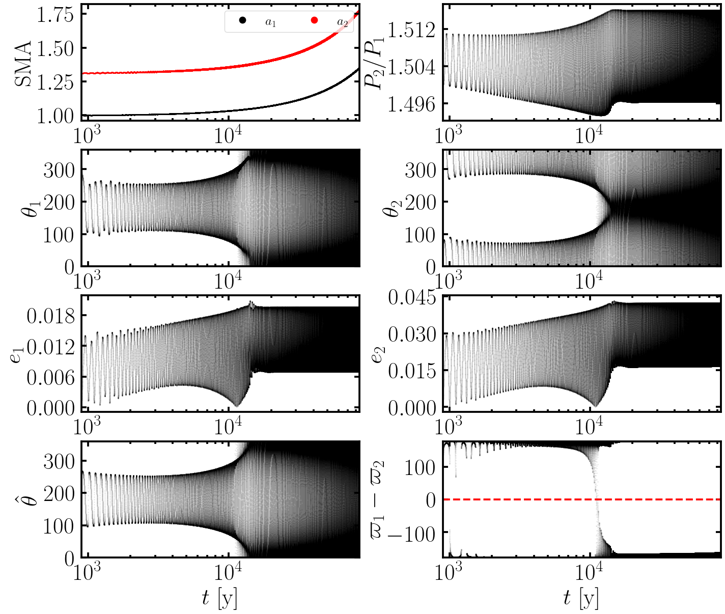
Figure 13: Same as Fig. 8, but with $e_{1d}=0$, $e_{2d}=0.1$. This system corresponds to the $\mathtt{x}$ marker in the top left panel of Fig. 12. The system starts off in resonance, with $\theta_{1}$, $\theta_{2}$ and $\hat{\theta}$ librating. However, after $10^{4}$ years, the system breaks out of all three resonances. Nevertheless, the period ratio remains locked around $1.5$ with small librations. The eccentricities reach the equilibrium values with large librations, while the apsidal angle $\Delta\varpi$ transitions from slightly less than $180^{\circ}$ to slightly larger than $180^{\circ}$.

Now that we have identified these three resonant modes, here we explore the $(e_{1d},e_{2d})$ parameter space for moderate values between $0$ and $0.2$. The top row of Fig. 12 shows the result for $q=2$, $h=0.03$, and initial period ratio $P_{2}/P_{1}=1.5$. In the left panel, we summarize the resonant behavior for each system on an $e_{1,d}$-$e_{2,d}$ grid. We mark the run which becomes unstable and escapes the resonance within the timescale of our integration by an $\mathtt{x}$ marker. Roughly, for $e_{1d}\gtrsim e_{2d}$, the system becomes apsidally aligned ($\Delta\varpi=0^{\circ}$). For $e_{2d}>e_{1d}$, one case exhibits $\Delta\varpi=90^{\circ}$, one escapes, and the others are apsidally anti-aligned. In the right panel of Fig. 12, we plot the time-averaged final eccentricities of the planets. The points share the same color-coding as in the left panel. The eccentricities for the aligned cases fall roughly along the line $e_{1}=e_{2}$, which reflects the fact that the angle $\hat{\theta}$ does not depend on the mass ratio $q$ (equation 39). The perpendicular case ($\Delta\varpi=90^{\circ}$) falls slightly above the line $e_{2}/e_{1}=q$, while the anti-aligned runs fall just under it.

The single $\mathtt{x}$ marker in the top left panel of Fig. 12 corresponds to a run which is only temporarily caught into resonance. We show the detailed evolution of this system in Fig. 13. Although all resonance angles circulate, the period ratio librates with a small amplitude around $P_{2}/P_{1}=1.5$. The planets remain in an anti-aligned configuration throughout. Before the escape, $\Delta\varpi\lesssim 180^{\circ}$, while after the escape, $\Delta\varpi\gtrsim 180^{\circ}$.

4.5 Initial period ratio

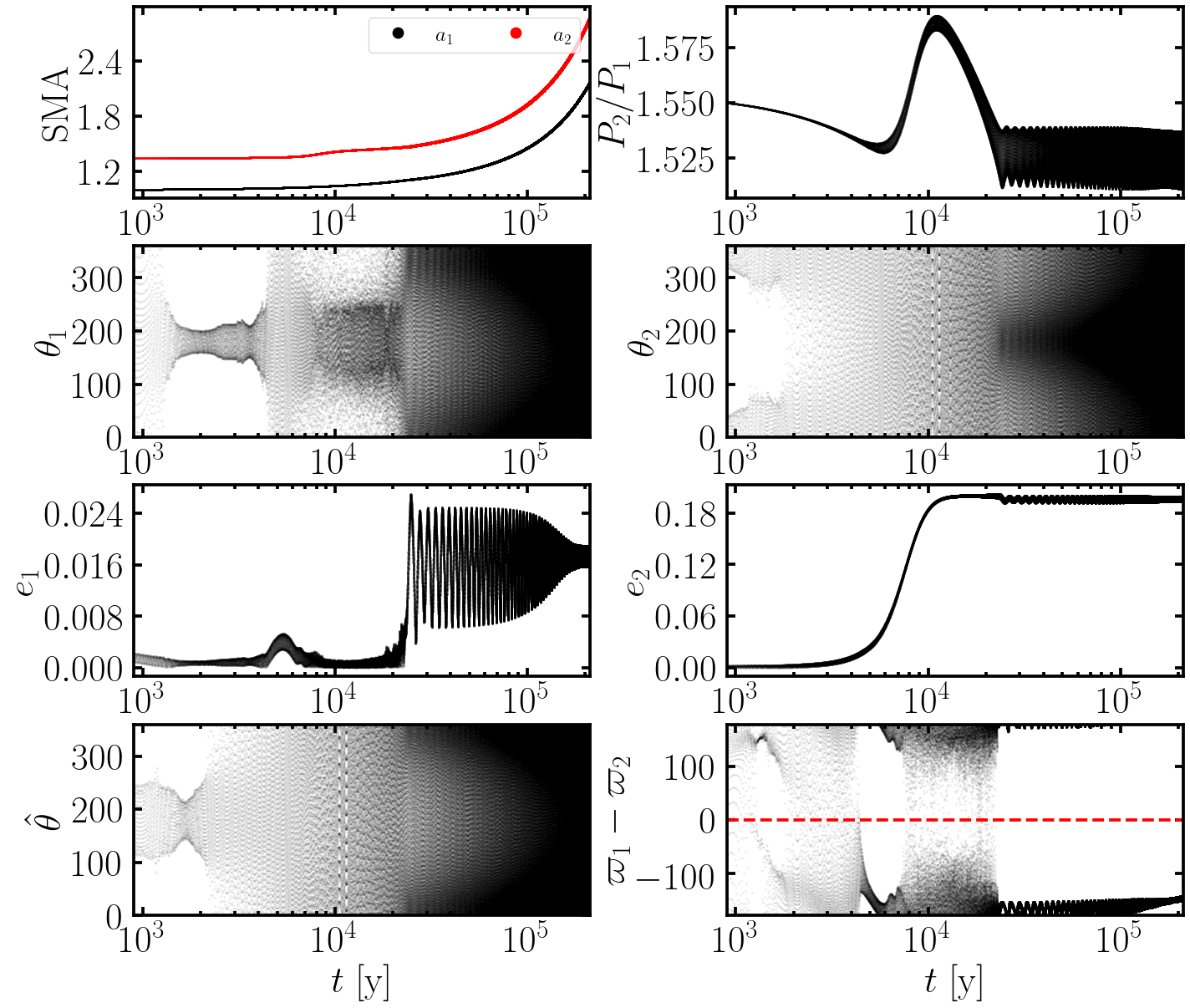
Figure 14: Same as Fig. 8 (for $q=2$) but with $e_{1d}=0$ and $e_{2d}=0.2$ and an initial period ratio of $P_{2}/P_{1}=1.55$. The system corresponds to one of the $\mathtt{x}$ marks in the left, second row of Fig. 12. The period ratio initially decreases as the planets migrate convergently. Around $t=10^{4}$ years, the period ratio increases, then again turns around and settles down into libration around 1.525, while all resonant angles circulate.

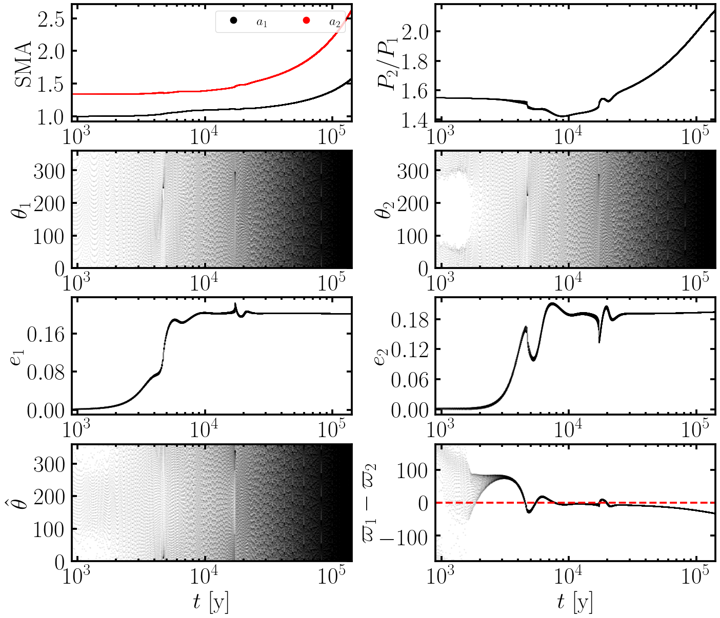
Figure 15: Same as Fig. 14, but with $e_{1d}=0.2$ and $e_{2d}=0.2$. This corresponds to one of the $\mathtt{x}$ marks in the left, second row of Fig. 12. The system convergently migrates outward for some time, after which it crosses the resonance location without being captured (i.e., the kink between $t=3000$ and 4000 years). The period ratio then turns around and misses the resonance again, after which it continues to grow for the rest of the integration. In this example, as opposed to Fig. 14, the resonance angles never appear to librate.

In the second row of Fig. 12, we have kept all of the parameters from the first row constant, but shifted the initial location of $m_{2}$ so that $P_{2}/P_{1}=1.55$. As we can see from the left panel, many more systems fail to be permanently captured.

Fig. 14 displays the result of a system which fails to be captured in the resonance. We see that after a short period of convergent migration, the outer planet is repelled away from the resonance. Following an initial decrease, the period ratio increases and then turns around and levels off into a state which resembles the late-time behavior in Fig. 13.

Fig. 15 depicts another example of failed resonance capture. Initially, both planets undergo convergent outward migration, but after some time, $a_{1}$ begins to increase. Then, the planets skip the resonance as the period ratio passes through $P_{2}/P_{1}=1.5$ from above. It continues decreasing, turns around, and then skips the resonance from below.

4.6 Mass ratio

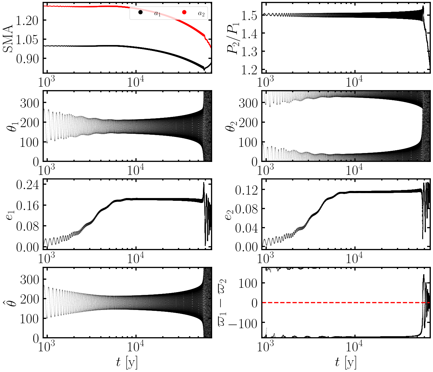
Figure 16: Same as Fig. 14, but with $q=0.5$, $e_{1d}=0.2$, $e_{2d}=0.1$ and an initial period ratio $P_{2}/P_{1}=1.5$. This corresponds to one of the $\mathtt{x}$ marks in the left, third row of Fig. 12. The planets are caught into all three resonances for most of the integration. The period ratio is likewise locked near 1.5 with libration that grows slightly over time. Then the system exits all three resonances at the same time, after which $m_{1}$ launches outwards leading to eventual orbit-crossing.

Now we turn to the effect of mass ratio on the resonance capture. Rows three and four of Fig. 12 summarize the results of running identical integrations to the first two rows but setting $q=0.5$, reversing the migration direction, and modifying the dissipation timescales appropriately. Only one system out of the 18 in the last two rows of Fig. 12 becomes apsidally aligned, while for all cases with $e_{2,d}=0$, the planets are anti-aligned. The top-left-most points (i.e. $e_{2,d}>e_{1,d}$) all escape the resonance whenever $q<1$.

In Fig. 16, we display the result of a system from the third row of Fig. 12. It has $e_{1d}=0.2$, $e_{2d}=0.1$, and an initial period ratio $P_{2}/P_{1}=1.5$. At the beginning of the integration, the two planets convergently migrate in resonance. Librations in the period ratio grow in amplitude over time. Eventually, the planets escape the resonance. The inner planet $m_{1}$ is kicked outwards and $m_{2}$ continues migrating inwards until the two planets’ orbits cross. This behavior could be related to the instability discovered for an inner test particle in the MMR capture (Goldreich & Schlichting, 2014; Xu et al., 2018).

4.7 Test particle limit

4.7.1 Relationship to the comparable mass case

The test particle Hamiltonian in equation (3) can also be transformed into the form of equation (38) through a canonical shift, analagous to the reducing rotation utilized in Section 4.2. Relative to the comparable mass case, the test-particle analysis is simpler because the vector $\mathbf{e}_{p}$ remains constant in time. Because of this, we now return to the test particle treatment of Section 3, with the goal of obtaining a heuristic understanding of apsidal alignment in real planetary systems (i.e. $0<q<\infty$).

For simplicity, we restrict ourselves to the case of an exterior test particle (as in Fig. 7), which is equivalent to the formal limit of $q=m_{1}/m_{2}\to\infty$. We now compare the $q=\infty$ case to the $q=2$ case, the latter of which we have investigated in Section 4 (i.e. the first two rows Fig. 12). Traversing Figure 7 along the $e_{p}$ axis is equivalent to traversing the $e_{1,\rm d}$ axis in Fig. 12. However, the vertical axis of Fig. 7 ($h$) is not equivalent to the vertical axis in Fig. 12 ($e_{2,\rm d}$). To relate these two quantities, we use $e_{\rm eq}$ $=h\sqrt{1.73/j}$ (equation 36) as a proxy for the “disk-driven eccentricity” of the test particle. One can see in Fig. 12 that, for the $q=2$ systems that do not escape, the division between “$\varpi-\text{aligned}$” and “$\varpi-\text{anti-aligned}$” roughly corresponds with the division between “$\varpi-\text{aligned}$” and “$\varpi-\text{circulating}$” for the test particle systems in Fig. 7. In the following, we treat “$\varpi-\text{circulating}$” and “$\varpi-\text{anti-aligned}$” as being equivalent dynamical states.

4.7.2 The condition for apsidal alignment

We again adopt the notation used in Section 3 for $q=\infty$. The resonant angle $\hat{\theta}$ can now be written as

$$\tan\hat{\theta}=\frac{e\sin\theta}{e\cos\theta-|f_{1}/f_{2}|e_{p}\cos\theta_{p}},$$ (44)

which is the test-particle limit of equation (39) (see Appendix B for details), where we have assumed $\varpi_{p}=0$. In both the $\varpi-\text{aligned}$ and $\varpi-\text{circulating}$ cases, $\theta_{p}$ circulates and $\hat{\theta}$ (as written in equation 44) librates around $0^{\circ}$. However, $\theta$ librates around $180^{\circ}$ when $\varpi$ circulates, and it circulates when $\varpi$ librates around $0$. This can be understood using the test-particle Hamiltonian (equation 3): $\dot{\varpi}$ is proportional to $\cos\theta$, and so $\varpi$ cannot librate if $\theta$ remains close to $180^{\circ}$.

The angle $\theta$ therefore determines the behavior of $\Delta\varpi$ in resonance for a test particle. Consider equation (44): since $\hat{\theta}$ always librates around $0$, then $\tan\hat{\theta}$ remains finite; this implies that the denominator never reaches $0$. Because $\theta_{p}$ always circulates, $\cos\theta_{p}$ takes on values between $-1$ and $1$. Thus, when $\theta$ librates around $180^{\circ}$, the following condition is required for $\hat{\theta}$ to librate:

$$-e+\left|\frac{f_{1}}{f_{2}}\right|e_{p}<0.$$ (45)

We assume the eccentricity librates around a central eccentricity $e_{c}\simeq e_{\rm eq}+\Delta_{e}$, which defines the parameter $\Delta_{e}$, and substitute this into equation (45):

$$e_{\rm eq}>\left|\frac{f_{1}}{f_{2}}\right|e_{p}-\Delta_{e}.$$ (46)

Using equation (36) to relate $h$ and $e_{\rm eq}$, we estimate the transition to aligned perihelia to occurs for $h<h_{c}(e_{p})$, where $h_{c}$ is given by

$$h_{c}(e_{p})=\sqrt{\frac{j}{1.73}}\left(\left|\frac{f_{1}}{f_{2}}\right|e_{p}-\Delta_{e}\right)$$ (47)

In principle, $\Delta_{e}$ could be zero, but we find $\Delta_{e}=0.015$ to be a better approximation, which we use for the line in Figure 7. Despite the many approximations, this analysis reproduces the numerical results fairly well.

4.7.3 Discussion for $0<q<\infty$

The above analysis shows that test particle apsidal alignment can be understood as a competition between $e_{\rm eq}$, which is related to $h$, and $e_{p}$, the eccentricity of the massive planet. Our interpretation of this result in the comparable mass context is to identify the disc driven eccentricities $e_{1,d}$ and $e_{2,d}$ of Section 4 with $e_{\rm eq}$ and $e_{p}$ in Section 3.

Apsidal behavior in the comparable mass regime is more complex than the test-mass system. We observe that $|\Delta\varpi|=0$, $90^{\circ}$, and $180^{\circ}$ are all possible. Each planet’s eccentricity works on the other to anti-align their periapses in resonance. However, if disc forces drive them away from the ratio $e_{1}/e_{2}=1/q$, the tendency of anti-alignment can be overcome, resulting in a different apsidal configuration. The resulting configuration has a complicated dependence on the planet and disk parameters, with some systems escaping resonance (see Fig. 12). A detailed analysis of the effects of different parameters $q$, $h$, $T_{e}$, and $e_{i,d}$ would reveal transitions between the resonance modes analogous to equation (47) for the comparable mass regime.

5 Conclusion

We have studied the mean-motion resonance capture of two migrating planets in protoplanetary disks, focusing on the property of the apsidal angles of captured planets. Our study is motivated by recent observations, which show that planets in MMR can be either apsidally aligned or anti-aligned (see Section 1).

In the standard picture of MMR capture, planets undergo convergent migration and experience eccentricity damping due to planet-disk interactions. We show in Section 2 that this standard picture always leads to capture where the resonance angles, $\theta_{1}=(j+1)\lambda_{2}-j\lambda_{1}-\varpi_{1}$ and $\theta_{2}=(j+1)\lambda_{2}-j\lambda_{1}-\varpi_{2}$, librate around zero or $\pi$, and such capture produces apsidal anti-alignment ($\Delta\varpi=\varpi_{1}-\varpi_{2}=180^{\circ}$).

To explore the possibility of producing apsidal alignment in MMR capture, we analyze the problem of a test particle in the vicinity of an MMR with a planet of mass $m_{p}$ (Section 3). We find that apsidal alignment occurs when the planet’s eccentricity $e_{p}$ is comparable or larger than the “equilibrium” eccentricity of the test particle captured in MMR (see Fig. 7), the latter results from the migration and eccentricty damping by the disc, and depends on the disc apsect ratio $h$ (see Eq. 37).

Our test particle results inform our analysis of how apsidal alignment may arise in the case of comparable-mass planets. In Section 4, we show that when the planets experience eccentricity driving due to their interactions with the disc, apsidal alignment in MMR capture can be produced. The eccentricity driving forces prevent the libration of $\theta_{1}$ and $\theta_{2}$, allowing the captured planets to settle into the apsidally aligned state (see Fig. 8) in which a “mixed” resonant angle $\hat{\theta}$ librates. However, in the presence of eccentricity driving, the process of MMR capture is highly irregular; depending on the initial condition, the planet mass ratio, and the magntitudes of the driving forces, various outcomes can be produced, including apsidal alignment, anti-alignment, and a perpendicular configuration ($\Delta\varpi=90^{\circ}$), as well as resonance disruption (see Fig. 12).

This paper represents the first investigation into the effect of eccentricity driving in mean-motion resonant systems. The observed apsidal alignment in the K2-19 system, the moderate eccentricites of K2-19b and c, and the libration of the “mixed” resonant angle ($\hat{\theta}$; Petit et al., 2020), can all be produced by this effect. These suggest that the planets in the K2-19 system have interacted with an eccentricity driving disc in the past. In addition, our finding that MMR capture can be disrupted by eccentricity driving may also contribute to the observed underabundance of exact MMRs (with $P_{2}/P_{1}=(j+1)/j$) in the Kepler multi-planet systems (Fabrycky et al., 2014), simply because the exact resonant systems can be pushed to slightly larger period ratios whenever the disc drives the planet eccentricities.

Our results come with the obvious caveat that we have used simple parameterized models (with constant dissipative timescales) for the planetary eccentricity damping and driving by the disc. In reality, the coupling between the disc and planet is a function of eccentricity, location in the disk, and disc profile. Long-term hydrodynamical simulations of two migrating planets in discs, including the possibility of eccentricity driving, would be needed to fully explore the effects studied in this paper.

Data Availability

The code used to generate the data for this paper can be found on https://github.com/jtlaune/mmr-apsidal-angle. All figures can be reproduced from this data.

Appendix A Comparable mass Hamiltonian

A.1 Scaling the Hamiltonian

The Hamiltonian for two comparable mass planets near the $j:j+1$ resonance is

$$H=-\frac{GMm_{1}}{2a_{1}}-\frac{GMm_{2}}{2a_{2}}-\frac{Gm_{1}m_{2}}{a_{2}}\left[f_{1}e_{1}\cos\theta_{1}+f_{2}e_{2}\cos\theta_{2}\right],$$ (48)

where $\theta_{1}=(j+1)\lambda_{2}-j\lambda_{1}-\varpi_{1}$ and $\theta_{2}=(j+1)\lambda_{2}-j\lambda_{1}-\varpi_{2}$ (equations 1 and 2) are the resonance angles and $f_{1}>0$, $f_{2}<0$ (equations 11 and 12) are functions of the SMA ratio, $\alpha=a_{1}/a_{2}$. Define $m_{\rm tot}=m_{1}+m_{2}$ and let $a_{0}$ be the scale length of the problem. We will then scale the Hamiltonian by $H_{0}=GMm_{\rm tot}/a_{0}$, the time by the frequency $\omega_{0}=\sqrt{GM/a_{0}^{3}}$, and the canonical momenta by $\Lambda_{0}=m_{\rm tot}\sqrt{GMa_{0}}$. The dimensionless Hamiltonian $\mathcal{H}$ is then

$$\mathcal{H}\equiv\frac{H}{H_{0}}=-\frac{m_{1}/m_{\rm tot}}{2a_{1}/a_{0}}-\frac{m_{2}/m_{\rm tot}}{2a_{2}/a_{0}}-\frac{\tilde{m}}{M(a_{2}/a_{0})}\left[f_{1}e_{1}\cos\theta_{1}+f_{2}e_{2}\cos\theta_{2}\right],$$ (49)

where $\tilde{m}=m_{1}m_{2}/m_{\rm tot}$ is the reduced mass. We assume the reduced mass ratio is small ($\tilde{\mu}=\tilde{m}/M\ll 1$). The canonical momenta, coordinate pairs are

$$\Lambda_{1} =\frac{m_{1}}{m_{\rm tot}}\sqrt{\frac{a_{1}}{a_{0}}},\quad\lambda_{1},$$ (50)

$$\Lambda_{2} =\frac{m_{2}}{m_{\rm tot}}\sqrt{\frac{a_{2}}{a_{0}}},\quad\lambda_{1},$$ (51)

$$\Gamma_{1} =\frac{m_{1}}{m_{\rm tot}}\sqrt{\frac{a_{1}}{a_{0}}}\left(1-\sqrt{1-e_{2}^{2}}\right),\quad\gamma_{1},$$ (52)

$$\Gamma_{2} =\frac{m_{2}}{m_{\rm tot}}\sqrt{\frac{a_{2}}{a_{0}}}\left(1-\sqrt{1-e_{2}^{2}}\right),\quad\gamma_{2},$$ (53)

where $\gamma_{1}=-\varpi_{1}$ and $\gamma_{2}=-\varpi_{2}$. The Hamiltonian can be expressed as a function of the momenta and resonance angles,

$$\mathcal{H}=-\frac{q^{3}}{2(1+q)^{3}\Lambda_{1}^{2}}-\frac{1}{2(1+q)^{3}\Lambda_{2}^{2}}-\frac{\tilde{\mu}}{(1+q)^{2}\Lambda_{2}^{2}}\left[f_{1}\sqrt{\frac{2\Gamma_{1}}{\Lambda_{1}}}\cos\theta_{1}+f_{2}\sqrt{\frac{2\Gamma_{2}}{\Lambda_{2}}}\cos\theta_{2}\right],$$ (54)

where we have used $q=m_{1}/m_{2}$.

A.2 Transforming the Hamiltonian

We would like to find the momenta conjugate to the fast coordinates $\lambda_{i}$ while making the slowly varying $\theta_{i}$ conjugate to $\Gamma_{i}$. Such a canonical transformation preserves the form

$$d\mathcal{H} =\Lambda_{1}d\lambda_{1}+\Lambda_{2}d\lambda_{2}+\Gamma_{1}d\gamma_{1}+\Gamma_{2}d\gamma_{2}$$

$$=\Gamma_{1}d\theta_{1}+\Gamma_{2}d\theta_{2}+J_{1}d\lambda_{1}+J_{2}d\lambda_{2}.$$ (55)

We can solve the set of equations in (A.2) for

$$J_{1} =\Lambda_{1}+j(\Gamma_{1}+\Gamma_{2}),$$ (56)

$$J_{2} =\Lambda_{2}-(j+1)(\Gamma_{1}+\Gamma_{2}),$$ (57)

where $\Gamma_{i}$ and $J_{i}$ are now conjugate to $\theta_{i}$ and $\lambda_{i}$, respectively. The coordinates $\lambda_{1}$ and $\lambda_{2}$ no longer appear in the Hamiltonian, which means $J_{1}$ and $J_{2}$ are constants of motion and equation (54) may be written in the following form:

$$\mathcal{H}=\mathcal{H}_{0}(\Gamma_{1}+\Gamma_{2};J_{1},J_{2},q)+\mathcal{H}_{\rm pert}(\theta_{1},\theta_{2},\Gamma_{1},\Gamma_{2};J_{1},J_{2},q),$$ (58)

where

$$\mathcal{H}_{0}(\Gamma_{1}+\Gamma_{2};J_{1},J_{2},q)=-\frac{q^{3}}{2(1+q)^{3}(J_{1}-j(\Gamma_{1}+\Gamma_{2}))^{2}}-\frac{1}{2(1+q)^{3}(J_{2}+(j+1)(\Gamma_{1}+\Gamma_{2}))^{2}}$$ (59)

and

$$\mathcal{H}_{\rm pert}(\Gamma_{1},\Gamma_{2};J_{1},J_{2},q)=-\frac{\tilde{\mu}}{(1+q)^{2}(J_{2}+(j+1)(\Gamma_{1}+\Gamma_{2}))^{2}}\left[f_{1}\sqrt{\frac{2\Gamma_{1}}{J_{1}-j(\Gamma_{1}+\Gamma_{2})}}\cos\theta_{1}+f_{2}\sqrt{\frac{2\Gamma_{2}}{J_{2}+(j+1)(\Gamma_{1}+\Gamma_{2})}}\cos\theta_{2}\right].$$ (60)

We have $\Gamma_{i}\ll\Lambda_{i}$ for small eccentricities. Under this assumption, we may drop terms smaller than $\mathcal{O}(\Gamma_{i}^{2}/\Lambda_{i}^{4})$. Equation (59) becomes

$$\mathcal{H}_{0}=\mathcal{C}_{0}(q,J_{1},J_{2})-\frac{1}{(1+q)^{3}}\left[\frac{q^{3}}{2\Lambda_{1}^{2}}+\frac{1}{2\Lambda_{2}^{2}}+\left(\frac{jq^{3}}{\Lambda_{1}^{3}}-\frac{(j+1)}{\Lambda_{2}^{3}}\right)(\Gamma_{1}+\Gamma_{2})-\frac{3}{2}\left(\frac{j^{2}q^{3}}{\Lambda_{1}^{4}}-\frac{(j+1)^{2}}{\Lambda_{2}^{4}}\right)(\Gamma_{1}+\Gamma_{2})^{2}\right],$$ (61)

where $\mathcal{C}_{0}$ is a constant of resonance which depends on initial conditions. Hence, we leave $\mathcal{C}_{0}$ out of the following calculations. Absent any dissipation, $\Lambda_{1}$ and $\Lambda_{2}$ are approximately constant in resonance. Hence, we may also drop the first two terms in parentheses in equation (61), leaving only the terms which include factors of $(\Gamma_{1}+\Gamma_{2})$:

$$\mathcal{H}_{0}=-\frac{1}{(1+q)^{3}}\left[\left(\frac{jq^{3}}{\Lambda_{1}^{3}}-\frac{(j+1)}{\Lambda_{2}^{3}}\right)(\Gamma_{1}+\Gamma_{2})-\frac{3}{2}\left(\frac{j^{2}q^{3}}{\Lambda_{1}^{4}}-\frac{(j+1)^{2}}{\Lambda_{2}^{4}}\right)(\Gamma_{1}+\Gamma_{2})^{2}\right].$$ (62)

The perturbation part (equation 60) reduces to its original form,

$$\mathcal{H}_{\rm pert}=-\frac{\tilde{\mu}}{(1+q)^{2}\Lambda_{2}^{2}}\left[f_{1}\sqrt{\frac{2\Gamma_{1}}{\Lambda_{1}}}\cos\theta_{1}+f_{2}\sqrt{\frac{2\Gamma_{2}}{\Lambda_{2}}}\cos\theta_{2}\right],$$ (63)

because there is already a small factor ($\tilde{\mu}$) in the numerator.

A.3 Reducing rotation

Following Henrard et al. (1986) (equivalently, Wisdom, 1986; Deck et al., 2013; Moutamid et al., 2014), let $\boldsymbol{X}$ be the Cartesian formulation

$$\boldsymbol{X} =(x_{1},x_{2},X_{1},X_{2})$$

$$=(\sqrt{\Gamma_{1}}\cos\theta_{1},\sqrt{\Gamma_{2}}\cos\theta_{2},\sqrt{\Gamma_{1}}\sin\theta_{1},\sqrt{\Gamma_{2}}\sin\theta_{2})$$ (64)

Define

$$g_{1} =f_{1}\sqrt{\frac{2}{\Lambda_{1}}},$$ (65)

$$g_{2} =f_{2}\sqrt{\frac{2}{\Lambda_{2}}},$$ (66)

and

$$\mathcal{A}=\frac{1}{\sqrt{g_{1}^{2}+g_{2}^{2}}}.$$ (68)

The perturbation Hamiltonian, $\mathcal{H}_{\rm pert}$ (equation 63), has

$$\mathcal{H}_{\rm pert}\propto g_{1}x_{1}+g_{2}x_{2}.$$ (69)

Let $\boldsymbol{\Psi}$ be the counter-clockwise phase space rotation by the angle $\psi$, where $\tan\psi=g_{2}/g_{1}$,

$$\boldsymbol{\Psi}=\mathcal{A}\begin{pmatrix}g_{1}&g_{2}\\ -g_{2}&g_{1}\end{pmatrix}.$$ (70)

The block matrix

$$\boldsymbol{M}=\begin{pmatrix}\boldsymbol{\Psi}&\boldsymbol{0}\\ \boldsymbol{0}&\boldsymbol{\Psi}\end{pmatrix}$$ (71)

is symplectic (Goldstein et al., 2000). The coefficients $g_{i}$ depend weakly on the semimajor axis ratio $\alpha$, and so $\boldsymbol{M}$ only represents a canonical transformation if $\alpha$ is stationary or varying slowly, which is a good approximation for the systems considered in this paper.

Define the coordinates

$$\boldsymbol{W}=(w_{1},w_{2},W_{1},W_{2})\equiv\boldsymbol{M}\boldsymbol{X}.$$ (72)

so that $w_{1}=\mathcal{A}(g_{1}x_{1}+g_{2}x_{2})$. Hence, $\mathcal{H}_{\rm pert}\propto w_{1}$ only. Finally, we revert the $\boldsymbol{W}$ set back to polar coordinates $(\hat{\theta},\hat{\theta}_{2},S_{1}^{\prime},S_{2}^{\prime})$, so that $\mathcal{H}_{\rm pert}\propto\sqrt{S^{\prime}_{1}}\cos\hat{\theta}$ only. The sum

$$\Gamma_{1}+\Gamma_{2}=x_{1}^{2}+x_{2}^{2}+X_{1}^{2}+X_{2}^{2}=w_{1}^{2}+w_{2}^{2}+W_{1}^{2}+W_{2}^{2}=S^{\prime}_{1}+S^{\prime}_{2}$$ (73)

is preserved, and so the form of $\mathcal{H}_{0}$ is preserved:

$$\mathcal{H}_{0}=-\frac{1}{(1+q)^{3}}\left[\left(\frac{jq^{3}}{\Lambda_{1}^{3}}-\frac{(j+1)}{\Lambda_{2}^{3}}\right)(S^{\prime}_{1}+S^{\prime}_{2})-\frac{3}{2}\left(\frac{j^{2}q^{3}}{\Lambda_{1}^{4}}-\frac{(j+1)^{2}}{\Lambda_{2}^{4}}\right)(S^{\prime}_{1}+S^{\prime}_{2})^{2}\right].$$ (74)

The perturbation part is now

$$\mathcal{H}_{\rm pert}=-\frac{\tilde{\mu}}{(1+q)^{2}\Lambda_{2}^{2}}\sqrt{S^{\prime}_{2}}\cos\hat{\theta}.$$ (75)

The new resonance angle is given by the equation

$$\tan\hat{\theta}=\frac{W_{1}}{w_{1}}=\frac{f_{1}e_{1}\sin(\theta_{1})+f_{2}e_{2}\sin(\theta_{2})}{f_{1}e_{1}\cos(\theta_{1})+f_{2}e_{2}\cos(\theta_{2})}$$ (76)

and is conjugate to the momentum

$$S_{1}^{\prime}=w_{1}^{2}+W_{1}^{2}=\mathcal{A}^{2}(f_{1}^{2}e_{1}^{2}+2f_{1}f_{2}e_{1}e_{2}\cos(\varpi_{1}-\varpi_{2})+f_{2}^{2}e_{2}^{2}).$$ (77)

After the reducing rotation, neither $\mathcal{H}_{0}$ nor $\mathcal{H}_{\rm pert}$ depend on $\hat{\theta}_{2}$, and so its conjugate momentum, $S_{2}$, is a constant of resonance:

$$S_{2}^{\prime}=w_{2}^{2}+W_{2}^{2}=\mathcal{A}^{2}\left(q\sqrt{\alpha}f_{2}^{2}e_{1}^{2}-2f_{1}f_{2}e_{1}e_{2}\cos(\varpi_{1}-\varpi_{2})+\frac{f_{1}^{2}}{q\sqrt{\alpha}}e_{2}^{2}\right).$$ (78)

Through a scale transformation (which changes the time units by a factor of $1/\mathcal{A}^{2}$), we can remove the $\mathcal{A}^{2}$ term in $S^{\prime}_{1}$ and $S^{\prime}_{2}$. This results in the momentum

$$\hat{R}=\frac{1}{\mathcal{A}^{2}}S^{\prime}_{1}=f_{1}^{2}e_{1}^{2}-2|f_{1}f_{2}|e_{1}e_{2}\cos(\varpi_{1}-\varpi_{2})+f_{2}^{2}e_{2}^{2}$$ (79)

and conserved quantity

$$S_{2}=\frac{1}{\mathcal{A}^{2}}S^{\prime}_{2}=q\sqrt{\alpha}f_{2}^{2}e_{1}^{2}+2|f_{1}f_{2}|e_{1}e_{2}\cos(\varpi_{1}-\varpi_{2})+\frac{f_{1}^{2}}{q\sqrt{\alpha}}e_{2}^{2},$$ (80)

where we have used the fact $f_{1}f_{2}=-|f_{1}f_{2}|$. $\hat{R}$ has the following geometric interpretation:

$$\hat{R}=\left\lvert|f_{1}|\mathbf{e}_{1}-|f_{2}|\mathbf{e}_{2}\right\rvert^{2},$$ (81)

where the $\mathbf{e}_{i}$ are the Runge-Lenz vectors with magnitude $e_{i}$ in the direction of $\varpi_{i}$. The key characteristic of the $\hat{R}$, $\hat{\theta}$ conjugate pair is that it does not depend on the planetary mass ratio (e.g. Deck et al., 2013).

Altogether, we arrive at the following Hamiltonian after dropping constant terms:

$$\mathcal{H}(\hat{\theta},\hat{R}) =\mathcal{H}_{0}(\hat{R})+\mathcal{H}_{\rm pert}(\hat{\theta},\hat{R}),$$ (82)

$$\mathcal{H}_{0} =\left(3\mathcal{N}\mathcal{A}^{2}S_{2}-\mathcal{M}\right)\mathcal{A}^{2}\hat{R}-\frac{3}{2}\mathcal{N}\mathcal{A}^{4}\hat{R}^{2},$$ (83)

$$\mathcal{H}_{\rm pert} =-\tilde{\mu}\mathcal{K}\mathcal{A}\sqrt{\hat{R}}\cos\hat{\theta},$$ (84)

with coefficients given by

$$\mathcal{M} =\frac{1}{(1+q)^{3}}\left(\frac{jq^{3}}{\Lambda_{1}^{3}}-\frac{j+1}{\Lambda_{2}^{3}}\right),$$ (85)

$$\mathcal{N} =\frac{1}{(1+q)^{3}}\left(\frac{j^{2}q^{3}}{\Lambda_{1}^{4}}-\frac{(j+1)^{2}}{\Lambda_{2}^{4}}\right),$$ (86)

$$\mathcal{K} =\frac{1}{(1+q)^{2}\Lambda_{2}^{2}}.$$ (87)

Appendix B Test particle Hamiltonian

The internal and external test particle limits are largely analagous, and so we focus on the external limit, with $q$ approaching infinity. The inner planet now has constant $m_{1}=m_{p}>0$, $a_{1}=a_{p}$, $e_{1}=e_{p}$, and $\varpi_{1}=\varpi_{p}$. We may arbitrarily set $\varpi_{p}=0$ due to rotational symmetry. The test particle has $m_{2}=0$, $a_{2}=a$, $e_{2}=e$, and $\varpi_{2}=\varpi$. We are again neglecting dissipative and secular effects in our analysis. After transforming to the dimensionless Poincairé elements $\Lambda=\sqrt{a/a_{p}}$ and $\Gamma=\Lambda(1-\sqrt{1-e^{2}})\approx\frac{1}{2}\Lambda e^{2}$, the Hamiltonian is

$$\mathcal{H} =-\frac{1}{2\Lambda^{2}}-\mu_{p}\left(f_{2}\sqrt{\frac{2\Gamma}{\Lambda}}\cos(\theta_{p}+\gamma)+f_{1}e_{p}\cos\theta_{p}\right),$$ (88)

where $\theta_{p}=(j+1)\lambda-jn_{p}t$ is now an explicit function of time. The coordinate $\gamma=-\varpi$ is conjugate to $\Gamma$. Utilizing the approximation that $\alpha$ is varying adiabatically, we can effectively treat $\Lambda$ and $f_{i}$ as constants while in resonance.

Because we are now dealing with a potential that is an explicit function of time, the test particle formulation is formally different than the comparable mass problem, which is defined only for the parameter range $0<q<\infty$. The canonical transformation described in Appendix A, which is generated by the infinitesimal rotation about the origin, must also formally change. The corresponding transformation here is generated by the infinitesimal translation towards the inner planet’s Runge-Lenz vector, $\mathbf{e_{p}}$.

We will reduce equation (88) to a single degree of freedom Hamiltonian. If $e_{p}=0$, the resonance angle is $\theta=\theta_{p}+\gamma$. For $e_{p}>0$, we will derive an angle $\hat{\theta}$, analagous to equation (76), which incorporates the value $e_{p}$. Similar to our comparable mass derivation, we first switch to Cartesian coordinates $\mathbf{X}=(X,Y)=(\sqrt{\Gamma}\cos\gamma,\sqrt{\Gamma}\sin\gamma)$ so that the Hamiltonian now becomes

$$\mathcal{H} =-\frac{1}{2\Lambda^{2}}-\mu_{p}\left(f_{2}\sqrt{\frac{2}{\Lambda}}X\cos\theta_{p}+f_{2}\sqrt{\frac{2}{\Lambda}}Y\sin\theta_{p}+f_{1}e_{p}\cos\theta_{p}\right).$$ (89)

The first and third term now have identical dependence on $\theta_{p}$. The transformation of $\mathbf{X}$ coordinates given by

$$X^{\prime} =X+\frac{f_{1}e_{p}}{f_{2}}\sqrt{\frac{2}{\Lambda}},$$ (90)

$$Y^{\prime} =Y,$$ (91)

induces a new canonically conjugate pair $\mathbf{X}^{\prime}=(X^{\prime},Y^{\prime})$. The Hamiltonian becomes

$$\mathcal{H} =-\frac{1}{2\Lambda^{2}}-\mu_{p}\left(f_{2}\sqrt{\frac{2}{\Lambda}}X^{\prime}\cos\theta_{p}+f_{2}\sqrt{\frac{2}{\Lambda}}Y^{\prime}\sin\theta_{p}\right).$$ (92)

Finally, returning back to the canonical polar coordinates,

$$\tan\hat{\gamma} =\frac{Y^{\prime}}{X^{\prime}}$$ (93)

$$=\frac{f_{2}e\sin\gamma}{f_{2}e\cos\gamma+f_{1}e_{p}},$$ (94)

$$\hat{\Gamma} =X^{\prime 2}+Y^{\prime 2}$$ (95)

$$=\Gamma+\frac{f_{1}e_{p}}{f_{2}}\sqrt{\frac{\Lambda\Gamma}{2}}+\frac{f_{1}^{2}}{f_{2}^{2}}\frac{\Lambda e_{p}^{2}}{2},$$ (96)

we may write the Hamiltonian as

$$\mathcal{H} =-\frac{1}{2\Lambda^{2}}-\mu_{p}\left(f_{2}\sqrt{\frac{2\hat{\Gamma}}{\Lambda}}\cos(\theta_{p}+\hat{\gamma})\right).$$ (98)

The derivation may now continue as if this were the CR3BP, which culminates with the following action-angle pair:

$$\hat{R}=\frac{2f_{2}^{2}}{\Lambda}\hat{\Gamma} =f_{1}^{2}e_{p}^{2}+2f_{2}f_{1}e_{p}e\cos\hat{\gamma}+f_{2}^{2}e^{2},$$ (99)

$$\hat{\theta} =\theta_{p}+\hat{\gamma}.$$ (100)

References

- Antoniadou & Libert (2020) Antoniadou K. I., Libert A.-S., 2020, Astronomy and Astrophysics, 640, A55
- Armstrong et al. (2015) Armstrong D. J., et al., 2015, Astronomy & Astrophysics, 582, A33
- Batygin & Morbidelli (2013) Batygin K., Morbidelli A., 2013, Astronomy & Astrophysics, 556, A28
- Chatterjee & Ford (2015) Chatterjee S., Ford E. B., 2015, The Astrophysical Journal, 803, 33
- Choksi & Chiang (2020) Choksi N., Chiang E., 2020, Monthly Notices of the Royal Astronomical Society, 495, 4192
- Cresswell & Nelson (2008) Cresswell P., Nelson R. P., 2008, Astronomy & Astrophysics, 482, 677
- Deck & Batygin (2015) Deck K. M., Batygin K., 2015, The Astrophysical Journal, 810, 119
- Deck et al. (2013) Deck K. M., Payne M., Holman M. J., 2013, The Astrophysical Journal, 774, 129
- Delisle & Laskar (2014) Delisle J.-B., Laskar J., 2014, Astronomy & Astrophysics, 570, L7
- Delisle et al. (2015) Delisle J.-B., Correia A. C. M., Laskar J., 2015, Astronomy & Astrophysics, 579, A128
- Fabrycky et al. (2014) Fabrycky D. C., et al., 2014, The Astrophysical Journal, 790, 146
- Goldreich & Sari (2003) Goldreich P., Sari R., 2003, The Astrophysical Journal, 585, 1024
- Goldreich & Schlichting (2014) Goldreich P., Schlichting H. E., 2014, The Astronomical Journal, 147, 32
- Goldreich & Tremaine (1979) Goldreich P., Tremaine S., 1979, The Astrophysical Journal, 233, 857
- Goldreich & Tremaine (1980) Goldreich P., Tremaine S., 1980, The Astrophysical Journal, 241, 425
- Goldstein et al. (2000) Goldstein Poole Sako 2000, Classical Mechanics, 3rd edn
- Henrard et al. (1986) Henrard J., Lemaitre A., Milani A., Murray C. D., 1986, Celestial Mechanics, 38, 335
- Holman et al. (2010) Holman M. J., et al., 2010, Science, 330, 51
- Izidoro et al. (2017) Izidoro A., Ogihara M., Raymond S. N., Morbidelli A., Pierens A., Bitsch B., Cossou C., Hersant F., 2017, Monthly Notices of the Royal Astronomical Society, 470, 1750
- Lin & Papaloizou (1979) Lin D. N. C., Papaloizou J., 1979, Monthly Notices of the Royal Astronomical Society, 186, 799
- Lithwick & Wu (2012) Lithwick Y., Wu Y., 2012, The Astrophysical Journal, 756, L11
- Moutamid et al. (2014) Moutamid M. E., Sicardy B., Renner S., 2014, Celestial Mechanics and Dynamical Astronomy, 118, 235
- Murray & Dermott (2000) Murray C. D., Dermott S. F., 2000, Solar System Dynamics. Cambridge University Press, Cambridge, doi:10.1017/CBO9781139174817, http://ebooks.cambridge.org/ref/id/CBO9781139174817
- Nelson (2018) Nelson R. P., 2018, in Deeg H. J., Belmonte J. A., eds, , Handbook of Exoplanets. Springer International Publishing, Cham, pp 2287–2317, doi:10.1007/978-3-319-55333-7_139, https://doi.org/10.1007/978-3-319-55333-7_139
- Petigura et al. (2018) Petigura E. A., et al., 2018, The Astronomical Journal, 156, 89
- Petigura et al. (2020) Petigura E. A., et al., 2020, The Astronomical Journal, 159, 2
- Petit et al. (2020) Petit A. C., Petigura E. A., Davies M. B., Johansen A., 2020, arXiv:2003.04931 [astro-ph]
- Ragusa et al. (2017) Ragusa E., Rosotti G., Teyssandier J., Booth R., Clarke C. J., Lodato G., 2017, Monthly Notices of the Royal Astronomical Society, 474, 4460
- Romero et al. (2021) Romero D. A. V., Masset F. S., Teyssier R., 2021, Monthly Notices of the Royal Astronomical Society, nil, nil
- Tanaka & Ward (2004) Tanaka H., Ward W. R., 2004, The Astrophysical Journal, 602, 388
- Teyssandier & Ogilvie (2017) Teyssandier J., Ogilvie G. I., 2017, Monthly Notices of the Royal Astronomical Society, 467, 4577
- Weiss et al. (2020) Weiss L. M., et al., 2020, The Astronomical Journal, 159, 242
- Wisdom (1986) Wisdom J., 1986, Celestial Mechanics, 38, 175
- Xu & Lai (2016) Xu W., Lai D., 2016, Monthly Notices of the Royal Astronomical Society, 459, 2925
- Xu et al. (2018) Xu W., Lai D., Morbidelli A., 2018, Monthly Notices of the Royal Astronomical Society, 481, 1538