: A Scalable Path-based Reasoning Approach for Knowledge Graphs

Abstract

Reasoning on large-scale knowledge graphs has been long dominated by embedding methods. While path-based methods possess the inductive capacity that embeddings lack, their scalability is limited by the exponential number of paths. Here we present , a scalable path-based method for knowledge graph reasoning. Inspired by the A* algorithm for shortest path problems, our learns a priority function to select important nodes and edges at each iteration, to reduce time and memory footprint for both training and inference. The ratio of selected nodes and edges can be specified to trade off between performance and efficiency. Experiments on both transductive and inductive knowledge graph reasoning benchmarks show that achieves competitive performance with existing state-of-the-art path-based methods, while merely visiting 10% nodes and 10% edges at each iteration. On a million-scale dataset ogbl-wikikg2, not only achieves a new state-of-the-art result, but also converges faster than embedding methods. is the first path-based method for knowledge graph reasoning at such scale.

1 Introduction

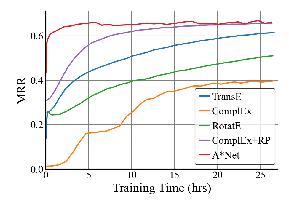
Figure 1: Validation MRR w.r.t. training time on ogbl-wikikg2 (1 A100 GPU). achieves state-of-the-art performance and the fastest convergence.

Reasoning, the ability to apply logic to draw new conclusions from existing facts, has been long pursued as a goal of artificial intelligence [32, 20]. Knowledge graphs encapsulate facts in relational edges between entities, and serve as a foundation for reasoning. Reasoning over knowledge graphs is usually studied in the form of knowledge graph completion, where a model is asked to predict missing triplets based on observed triplets in the knowledge graph. Such a task can be used to not only populate existing knowledge graphs, but also improve downstream applications like multi-hop logical reasoning [34], question answering [5] and recommender systems [53].

One challenge central to knowledge graph reasoning is the scalability of reasoning methods, as many real-world knowledge graphs [2, 44] contain millions of entities and triplets. Typically, large-scale knowledge graph reasoning is solved by embedding methods [6, 42, 38], which learn an embedding for each entity and relation to reconstruct the structure of the knowledge graph. Due to its simplicity, embedding methods have become the de facto standard for knowledge graphs with millions of entities and triplets. With the help of multi-GPU embedding systems [57, 56], they can further scale to knowledge graphs with billions of triplets.

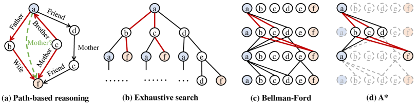
Figure 2: (a) Given a query $(a,\textit{Mother},?)$, only a few important paths (showed in red) are necessary for reasoning. Note that paths can go in the reverse direction of relations. (b) Exhaustive search algorithm (e.g., Path-RNN, PathCon) enumerates all paths in exponential time. (c) Bellman-Ford algorithm (e.g., NeuralLP, DRUM, NBFNet, RED-GNN) computes all paths in polynomial time, but needs to propagate through all nodes and edges. (d) learns a priority function to select a subset of nodes and edges at each iteration, and avoids exploring all nodes and edges.

Another stream of works, path-based methods [28, 31, 11, 58], predicts the relation between a pair of entities based on the paths between them. Take the knowledge graph in Fig. 2(a) as an example, we can prove that Mother(a, f) holds, because there are two paths a $\xrightarrow{\text{Father}}$ b $\xrightarrow{\text{Wife}}$ f and a $\xleftarrow{\text{Brother}}$ c $\xrightarrow{\text{Mother}}$ f. As the semantics of paths are purely determined by relations rather than entities, path-based methods naturally generalize to unseen entities (i.e., inductive setting), which cannot be handled by embedding methods. However, the number of paths grows exponentially w.r.t. the path length, which hinders the application of path-based methods on large-scale knowledge graphs.

Here we propose to tackle the scalability issue of path-based methods. The key idea of our method is to search for important paths rather than use all possible paths for reasoning, thereby reducing time and memory in training and inference. Inspired by the A* algorithm [22] for shortest path problems, given a head entity $u$ and a query relation $q$, we compute a priority score for each entity to guide the search towards more important paths. At each iteration, we select $K$ nodes and $L$ edges according to their priority, and use message passing to update nodes in their neighborhood. Due to the complex semantics of knowledge graphs, it is hard to use a handcrafted priority function like the A* algorithm without a significant performance drop (Tab. 6(a)). Instead, we design a neural priority function based on the node representations at the current iteration, which can be end-to-end trained by the objective function of the reasoning task without any additional supervision.

We verify our method on 4 transductive and 2 inductive knowledge graph reasoning datasets. Experiments show that achieves competitive performance against state-of-the-art path-based methods on FB15k-237, WN18RR and YAGO3-10, even with only 10% of nodes and 10% edges at each iteration (Sec. 4.2). To verify the scalability of our method, we also evaluate on ogbl-wikikg2, a million-scale knowledge graph that is 2 magnitudes larger than datasets solved by previous path-based methods. Surprisingly, with only 0.2% nodes and 0.2% edges, our method outperforms existing embedding methods and establishes new state-of-the-art results (Sec. 4.2) as the first non-embedding method on ogbl-wikikg2. By adjusting the ratios of selected nodes and edges, one can trade off between performance and efficiency (Sec. 4.3). also converges significantly faster than embedding methods (Fig. 1), which makes it a promising model for deployment on large-scale knowledge graphs. Additionally, offers interpretability that embeddings do not possess. Visualization shows that captures important paths for reasoning (Sec. 4.4).

2 Preliminary

Knowledge Graph Reasoning

A knowledge graph ${\mathcal{G}}=({\mathcal{V}},{\mathcal{E}},{\mathcal{R}})$ consists of sets of entities (nodes) ${\mathcal{V}}$, facts (edges) ${\mathcal{E}}$ and relation types ${\mathcal{R}}$. Each fact is a triplet $(x,r,y)\in{\mathcal{V}}\times{\mathcal{R}}\times{\mathcal{V}}$, which indicates a relation $r$ from entity $x$ to entity $y$. The task of knowledge graph reasoning aims at answering queries like $(u,q,?)$ or $(?,q,u)$. Without loss of generality, we assume the query is $(u,q,?)$, since $(?,q,u)$ equals to $(u,q^{-1},?)$ with $q^{-1}$ being the inverse of $q$. Given a query $(u,q,?)$, we need to predict the answer set ${\mathcal{V}}_{(u,q,?)}$, such that $\forall v\in{\mathcal{V}}_{(u,q,?)}$ the triplet $(u,q,v)$ should be true.

Path-based Methods

Path-based methods [28, 31, 11, 58] solve knowledge graph reasoning by looking at the paths between a pair of entities in a knowledge graph. For example, a path a $\xrightarrow{\text{Father}}$ b $\xrightarrow{\text{Wife}}$ f may be used to predict Mother(a, f) in Fig. 2(a). From a representation learning perspective, path-based methods aim to learn a representation ${\bm{h}}_{q}(u,v)$ to predict the triplet $(u,q,v)$ based on all paths ${\mathcal{P}}_{u\leadsto v}$ from entity $u$ to entity $v$. Following the notation in [58], ${\bm{h}}_{q}(u,v)$ is defined as

$${\bm{h}}_{q}(u,v)=\bigoplus_{P\in{\mathcal{P}}_{u\leadsto v}}{\bm{h}}_{q}(P)=\bigoplus_{P\in{\mathcal{P}}_{u\leadsto v}}\bigotimes_{(x,r,y)\in P}{\bm{w}}_{q}(x,r,y)$$ (1)

where $\bigoplus$ is a permutation-invariant aggregation function over paths (e.g., sum or max), $\bigotimes$ is an aggregation function over edges that may be permutation-sensitive (e.g., matrix multiplication) and ${\bm{w}}_{q}(x,r,y)$ is the representation of triplet $(x,r,y)$ conditioned on the query relation $q$. $\bigotimes$ is computed before $\bigoplus$. Typically, ${\bm{w}}_{q}(x,r,y)$ is designed to be independent of the entities $x$ and $y$, which enables path-based methods to generalize to the inductive setting. However, it is intractable to compute Eqn. 1, since the number of paths usually grows exponentially w.r.t. the path length.

Path-based Reasoning with Bellman-Ford algorithm

To reduce the time complexity of path-based methods, recent works [50, 35, 58, 54] borrow the Bellman-Ford algorithm [4] from shortest path problems to solve path-based methods. Instead of enumerating each possible path, the Bellman-Ford algorithm iteratively propagates the representations of $t-1$ hops to compute the representations of $t$ hops, which achieves a polynomial time complexity. Formally, let ${\bm{h}}_{q}^{(t)}(u,v)$ be the representation of $t$ hops. The Bellman-Ford algorithm can be written as

$${\bm{h}}_{q}^{(0)}(u,v)\leftarrow\text{1}_{q}(u=v)$$ (2)

$${\bm{h}}_{q}^{(t)}(u,v)\leftarrow{\bm{h}}_{q}^{(0)}(u,v)\oplus\bigoplus_{(x,r,v)\in{\mathcal{E}}(v)}{\bm{h}}_{q}^{(t-1)}(u,x)\otimes{\bm{w}}_{q}(x,r,v)$$ (3)

where $\text{1}_{q}$ is a learnable indicator function that defines the representations of $0$ hops ${\bm{h}}_{q}^{(0)}(u,v)$, also known as the boundary condition of the Bellman-Ford algorithm. ${\mathcal{E}}(v)$ is the neighborhood of node $v$. Despite the polynomial time complexity achieved by the Bellman-Ford algorithm, Eqn. 3 still needs to visit $|{\mathcal{V}}|$ nodes and $|{\mathcal{E}}|$ edges to compute ${\bm{h}}_{q}^{(t)}(u,v)$ for all $v\in{\mathcal{V}}$ in each iteration, which is not feasible for large-scale knowledge graphs.

A* Algorithm

A* algorithm [22] is an extension of the Bellman-Ford algorithm for shortest path problems. Unlike the Bellman-Ford algorithm that propagates through every node uniformly, the A* algorithm prioritizes propagation through nodes with higher priority according to a heuristic function specified by the user. With an appropriate heuristic function, A* algorithm can reduce the search space of paths. Formally, with the notation from Eqn. 1, the priority function for node $x$ is

$$s(x)=d(u,x)\otimes g(x,v)$$ (4)

where $d(u,x)$ is the length of current shortest path from $u$ to $x$, and $g(x,v)$ is a heuristic function estimating the cost from $x$ to the target node $v$. For instance, for a grid-world shortest path problem (Fig. 4(a)), $g(x,v)$ is usually defined as the $L_{1}$ distance from $x$ to $v$, $\otimes$ is the addition operator, and $s(x)$ is a lower bound for the shortest path length from $u$ to $v$ through $x$. During each iteration, the A* algorithm prioritizes propagation through nodes with smaller $s(x)$.

3 Proposed Method

We propose to scale up path-based methods with the A* algorithm. We show that the A* algorithm can be derived from the observation that only a small set of paths are important for reasoning (Sec. 3.1). Since it is hard to handcraft a good priority function for knowledge graph reasoning (Tab. 6(a)), we design a neural priority function, and train it end-to-end for reasoning (Sec. 3.2).

3.1 Path-based Reasoning with A* Algorithm

As discussed in Sec. 2, the Bellman-Ford algorithm visits all $|{\mathcal{V}}|$ nodes and $|{\mathcal{E}}|$ edges. However, in real-world knowledge graphs, only a small portion of paths is related to the query. Based on this observation, we introduce the concept of important paths. We then show that the representations of important paths can be iteratively computed with the A* algorithm under mild assumptions.

Important Paths for Reasoning

Given a query relation and a pair of entities, only some of the paths between the entities are important for answering the query. Consider the example in Fig. 2(a), the path a $\xrightarrow{\text{Friend}}$ d $\xrightarrow{\text{Mother}}$ e $\xrightarrow{\text{Friend}}$ f cannot determine whether f is an answer to Mother(a, ?) due to the use of the Friend relation in the path. On the other hand, kinship paths like a $\xrightarrow{\text{Father}}$ b $\xrightarrow{\text{Wife}}$ f or a $\xleftarrow{\text{Brother}}$ c $\xrightarrow{\text{Mother}}$ f are able to predict that Mother(a, f) is true. Formally, we define ${\mathcal{P}}_{u\leadsto v|q}\subseteq{\mathcal{P}}_{u\leadsto v}$ to be the set of paths from $u$ to $v$ that is important to the query relation $q$. Mathematically, we have

$${\bm{h}}_{q}(u,v)=\bigoplus_{P\in{\mathcal{P}}_{u\leadsto v}}{\bm{h}}_{q}(P)\approx\bigoplus_{P\in{\mathcal{P}}_{u\leadsto v|q}}{\bm{h}}_{q}(P)$$ (5)

In other words, any path $P\in{\mathcal{P}}_{u\leadsto v}\setminus{\mathcal{P}}_{u\leadsto v|q}$ has negligible contribution to ${\bm{h}}_{q}(u,v)$. In real-world knowledge graphs, the number of important paths $|{\mathcal{P}}_{u\leadsto v|q}|$ may be several orders of magnitudes smaller than the number of paths $|{\mathcal{P}}_{u\leadsto v}|$ [11]. If we compute the representation ${\bm{h}}_{q}(u,v)$ using only the important paths, we can scale up path-based reasoning to large-scale knowledge graphs.

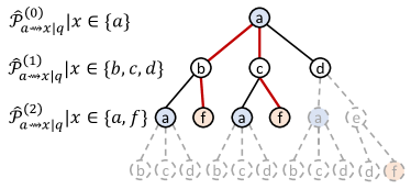
Figure 3: The colored paths are important paths ${\mathcal{P}}_{u\leadsto v|q}$, while the solid paths are the superset $\hat{{\mathcal{P}}}_{u\leadsto v|q}$ used in Eqn. 7.

Iterative Computation of Important Paths

Given a query $(u,q,?)$, we need to discover the set of important paths ${\mathcal{P}}_{u\leadsto v|q}$ for all $v\in{\mathcal{V}}$. However, it is challenging to extract important paths from ${\mathcal{P}}_{u\leadsto v}$, since the size of ${\mathcal{P}}_{u\leadsto v}$ is exponentially large. Our solution is to explore the structure of important paths and compute them iteratively. We first show that we can cover important paths with iterative path selection (Eqn. 6 and 7). Then we approximate iterative path selection with iterative node selection (Eqn. 8).

Notice that paths in ${\mathcal{P}}_{u\leadsto v}$ form a tree structure (Fig. 3). On the tree, a path is not important if any prefix of this path is not important for the query. For example, in Fig. 2(a), a $\xrightarrow{\text{Friend}}$ d $\xrightarrow{\text{Mother}}$ e $\xrightarrow{\text{Friend}}$ f is not important, as its prefix a $\xrightarrow{\text{Friend}}$ d is not important for the query Mother. Therefore, we assume there exists a path selection function $m_{q}:2^{\mathcal{P}}\mapsto 2^{\mathcal{P}}$ that selects important paths from a set of paths given the query relation $q$. $2^{\mathcal{P}}$ is the set of all subsets of ${\mathcal{P}}$. With $m_{q}$, we construct the following set of paths $\hat{{\mathcal{P}}}_{u\leadsto v|q}^{(t)}$ iteratively

$$\hat{{\mathcal{P}}}_{u\leadsto v|q}^{(0)}\leftarrow\{(u,\text{self loop},v)\}~{}\text{if}~{}u=v~{}\text{else}~{}\varnothing$$ (6)

$$\hat{{\mathcal{P}}}_{u\leadsto v|q}^{(t)}\leftarrow\bigcup_{\begin{subarray}{c}x\in{\mathcal{V}}\\ (x,r,v)\in{\mathcal{E}}(v)\end{subarray}}\left\{P+\{(x,r,v)\}\middle|P\in m_{q}(\hat{{\mathcal{P}}}_{u\leadsto x|q}^{(t-1)})\right\}$$ (7)

where $P+\{(x,r,v)\}$ concatenates the path $P$ and the edge $(x,r,v)$. The paths $\hat{{\mathcal{P}}}_{u\leadsto v|q}^{(t)}$ computed by the above iteration is a superset of the important paths ${\mathcal{P}}_{u\leadsto v|q}^{(t)}$ of length $t$ (see Thm. A.1 in App. A). Due to the tree structure of paths, the above iterative path selection still requires exponential time. Hence we further approximate iterative path selection with iterative node selection, by assuming paths with the same length and the same stop node can be merged. The iterative node selection replacing Eqn. 7 is (see Prop. A.3 in App. A)

$$\hat{{\mathcal{P}}}_{u\leadsto v|q}^{(t)}\leftarrow\bigcup_{\begin{subarray}{c}x\in n_{uq}^{(t-1)}({\mathcal{V}})\\ (x,r,v)\in{\mathcal{E}}(v)\end{subarray}}\left\{P+\{(x,r,v)\}\middle|P\in\hat{{\mathcal{P}}}_{u\leadsto x|q}^{(t-1)}\right\}$$ (8)

where $n_{uq}^{(t)}:2^{\mathcal{V}}\mapsto 2^{\mathcal{V}}$ selects ending nodes of important paths of length $t$ from a set of nodes.

Reasoning with A* Algorithm

Eqn. 8 iteratively computes the set of important paths $\hat{{\mathcal{P}}}_{u\leadsto v|q}$. In order to perform reasoning, we need to compute the representation ${\bm{h}}_{q}(u,v)$ based on the important paths, which can be achieved by an iterative process similar to Eqn. 8 (see Thm. A.4 in App. A)

$${\bm{h}}_{q}^{(t)}(u,v)\leftarrow {\bm{h}}_{q}^{(0)}(u,v)\oplus\bigoplus_{\begin{subarray}{c}x\in n_{uq}^{(t-1)}({\mathcal{V}})\\ (x,r,v)\in{\mathcal{E}}(v)\end{subarray}}{\bm{h}}_{q}^{(t-1)}(u,x)\otimes{\bm{w}}_{q}(x,r,v)$$ (9)

Eqn. 9 is the A* iteration (Fig. 2(d)) for path-based reasoning. Note the A* iteration uses the same boundary condition as Eqn. 2. Inspired by the classical A* algorithm, we parameterize $n_{uq}^{(t)}({\mathcal{V}})$ with a node priority function $s_{uq}^{(t)}:{\mathcal{V}}\mapsto[0,1]$ and select top-$K$ nodes based on their priority. However, there does not exist an oracle for the priority function $s_{uq}^{(t)}(x)$. We will discuss how to learn the priority function $s_{uq}^{(t)}(x)$ in the following sections.

3.2 Path-based Reasoning with

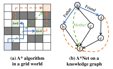
Figure 4: (a) A* algorithm computes the current distance $d(u,x)$ (blue), estimates the remaining distance $g(x,v)$ (orange), and prioritizes shorter paths. (b) A*Net computes the current representations ${\bm{h}}_{q}^{(t)}(u,x)$ (blue), estimates the remaining representations ${\bm{g}}([{\bm{h}}_{q}^{(t)}(u,x),{\bm{q}}])$ (orange) based on the query ${\bm{q}}$ (green), and prioritizes paths more relevant to the query.

Both the performance and the efficiency of the A* algorithm heavily rely on the heuristic function. While it is straightforward to use $L_{1}$ distance as the heuristic function for grid-world shortest path problems, it is not clear what a good priority function for knowledge graph reasoning is due to the complex relation semantics in knowledge graphs. Indeed, our experiments suggest that handcrafted priority functions largely hurt the performance of path-based methods (Tab. 6(a)). In this section, we discuss a neural priority function, which can be end-to-end trained by the reasoning task.

Neural Priority Function

To design the neural priority function $s_{uq}(x)$, we draw inspiration from the priority function in the A* algorithm for shortest path problems (Eqn. 4). The priority function has two terms $d(u,x)$ and $g(x,v)$, where $d(u,x)$ is the current distance from node $u$ to $x$, and $g(x,v)$ estimates the remaining distance from node $x$ to $v$.

From a representation learning perspective, we need to learn a representation ${\bm{s}}_{uq}(x)$ to predict the priority score $s_{uq}(x)$ for each node $x$. Inspired by Eqn. 4, we use the current representation ${\bm{h}}_{q}^{(t)}(u,x)$ to represent $d^{(t)}(u,x)$. However, it is challenging to find a representation for $g^{(t)}(x,v)$, since we do not know the answer entity $v$ beforehand. Noticing that in the A* algorithm, the target node $v$ can be expressed by the source node plus a displacement (Fig. 4(a)), we reparameterize the answer entity $v$ with the head entity $u$ and the query relation $q$ in . By replacing $g^{(t)}(x,v)$ with another function $g^{(t)}(u,x,q)$, the representation ${\bm{s}}_{uq}(x)$ is parameterized as

$${\bm{s}}_{uq}^{(t)}(x)={\bm{h}}_{q}^{(t)}(u,x)\otimes{\bm{g}}([{\bm{h}}_{q}^{(t)}(u,x),{\bm{q}}])$$ (10)

where ${\bm{g}}(\cdot)$ is a feed-forward network that outputs a vector representation and $[\cdot,\cdot]$ concatenates two representations. Intuitively, the learned representation ${\bm{q}}$ captures the semantic of query relation $q$, which serves the goal for answering query $(u,q,?)$. The function ${\bm{g}}([{\bm{h}}_{q}^{(t)}(u,x),{\bm{q}}])$ compares the current representation ${\bm{h}}_{q}^{(t)}(u,x)$ with the goal ${\bm{q}}$ to estimate the remaining representation (Fig. 4(b)). If ${\bm{h}}_{q}^{(t)}(u,x)$ is close to ${\bm{q}}$, the remaining representation will be close to 0, and $x$ is likely to be close to the correct answer. The final priority score is predicted by

$$s_{uq}^{(t)}(x)=\sigma(f({\bm{s}}_{uq}^{(t)}(x)))$$ (11)

where $f(\cdot)$ is a feed-forward network and $\sigma$ is the sigmoid function that maps the output to $[0,1]$.

Learning

To learn the neural priority function, we incorporate it as a weight for each message in the A* iteration. For simplicity, let ${\mathcal{X}}^{(t)}=n_{uq}^{(t-1)}({\mathcal{V}})$ be the nodes we try to propagate through at $t$-th iteration. We modify Eqn. 9 to be

$${\bm{h}}_{q}^{(t)}(u,v)\leftarrow{\bm{h}}_{q}^{(0)}(u,v)\oplus\bigoplus_{\begin{subarray}{c}x\in{\mathcal{X}}^{(t)}\\ (x,r,v)\in{\mathcal{E}}(v)\end{subarray}}s_{uq}^{(t-1)}(x)\left({\bm{h}}_{q}^{(t-1)}(u,x)\otimes{\bm{w}}_{q}(x,r,v)\right)$$ (12)

Eqn. 12 encourages the model to learn larger weights $s_{uq}^{(t)}(x)$ for nodes that are important for reasoning. In practice, as some nodes may have very large degrees, we further select top-$L$ edges from the neighborhood of $n_{uq}^{(t-1)}({\mathcal{V}})$ (see App. B). A pseudo code of is illustrated in Alg. 1. Note the top-$K$ and top-$L$ functions are not differentiable.

Nevertheless, it is still too challenging to train the neural priority function, since we do not know the ground truth for important paths, and there is no direct supervision for the priority function. Our solution is to share the weights between the priority function and the predictor for the reasoning task. The intuition is that the reasoning task can be viewed as a weak supervision for the priority function. Recall that the goal of $s_{uq}^{(t)}(x)$ is to determine whether there exists an important path from $u$ to $x$ (Eqn. 8). In the reasoning task, any positive answer entity must be present on at least one important path, while negative answer entities are less likely to be on important paths. Our ablation experiment demonstrates that sharing weights improve the performance of neural priority function (Tab. 6(b)). Following [38], is trained to minimize the binary cross entropy loss over triplets

$${\mathcal{L}}=-\log p(u,q,v)-\sum_{i=1}^{n}\frac{1}{n}\log(1-p(u_{i}^{\prime},q,v_{i}^{\prime}))$$ (13)

where $(u,q,v)$ is a positive sample and $\{(u_{i}^{\prime},q,v_{i}^{\prime})\}_{i=1}^{n}$ are negative samples. Each negative sample $(u_{i},q,v_{i})$ is generated by corrupting the head or the tail in a positive sample.

Algorithm 1

Input: head entity $u$, query relation $q$, #iterations $T$
Output: $p(v|u,q)$ for all $v\in{\mathcal{V}}$

1:for $v\in{\mathcal{V}}$ do

2:    ${\bm{h}}_{q}^{(0)}(u,v)\leftarrow\text{1}_{q}(u=v)$

3:end for

4:for $t\leftarrow 1$ to $T$ do

5:    ${\mathcal{X}}^{(t)}\leftarrow\textrm{TopK}(s_{uq}^{(t-1)}(x)|x\in{\mathcal{V}})$

6:    ${\mathcal{E}}^{(t)}\leftarrow\bigcup_{x\in{\mathcal{X}}^{(t)}}{\mathcal{E}}(x)$

7:    ${\mathcal{E}}^{(t)}\leftarrow\textrm{TopL}(s_{uq}^{(t-1)}(v)|(x,r,v)\in{\mathcal{E}}^{(t)})$

8:    ${\mathcal{V}}^{(t)}\leftarrow\bigcup_{(x,r,v)\in{\mathcal{E}}^{(t)}}\{v\}$

9:    for $v\in{\mathcal{V}}^{(t)}$ do

10:        Compute ${\bm{h}}_{q}^{(t)}(u,v)$ with Eqn. 12

11:        Compute priority $s_{uq}^{(t)}(v)$ with Eqn. 10, 11

12:    end for

13:end for

14:$\triangleright$ Share weights between $s_{uq}(v)$ and the predictor

15:return $s_{uq}^{(T)}(v)$ as $p(v|u,q)$ for all $v\in{\mathcal{V}}$

Efficient Implementation with Padding-Free Operations

Modern neural networks heavily rely on batched execution to unleash the parallel capacity of GPUs. While Alg. 1 is easy to implement for a single sample $(u,q,?)$, it is not trivial to batch for multiple samples. The challenge is that different samples may have very different sizes for nodes ${\mathcal{V}}^{(t)}$ and edges ${\mathcal{E}}^{(t)}$. A common approach is to pad the set of nodes or edges to a predefined constant, which would severely counteract the acceleration brought by .

Here we introduce padding-free $topk$ operation to avoid the overhead in batched execution. The key idea is to convert batched execution of different small samples into execution of a single large sample, which can be paralleled by existing operations in deep learning frameworks. For example, the batched execution of $topk([[1,3],[2,1,0]])$ can be converted into a multi-key sort problem over $[[0,1],[0,3],[1,2],[1,1],[1,0]]$, where the first key is the index of the sample in the batch and the second key is the original input. The multi-key sort is then implemented by composing stable single-key sort operations in deep learning frameworks. See App. C for details.

4 Experiments

We evaluate on standard transductive and inductive knowledge graph reasoning datasets, including a million-scale one ogbl-wikikg2. We conduct ablation studies to verify our design choices and visualize the important paths learned by the priority function in .

4.1 Experiment Setup

Datasets & Evaluation

We evaluate on 4 standard knowledge graphs, FB15k-237 [40], WN18RR [16], YAGO3-10 [30] and ogbl-wikikg2 [25]. For the transductive setting, we use the standard splits from their original works [40, 16]. For the inductive setting, we use the splits provided by [39], which contains 4 different versions for each dataset. As for evaluation, we use the standard filtered ranking protocol [6] for knowledge graph reasoning. Each triplet $(u,q,v)$ is ranked against all negative triplets $(u,q,v^{\prime})$ or $(u^{\prime},q,v)$ that are not present in the knowledge graph. We measure the performance with mean reciprocal rank (MRR) and HITS at K (H@K). Efficiency is measured by the average number of messages (#message) per step, wall time per epoch and memory cost. To plot the convergence curves for each model, we dump checkpoints during training with a high frequency, and evaluate the checkpoints later on the validation set. See more details in App. D.

Implementation Details

Our work is developed based on the open-source codebase of path-based reasoning with Bellman-Ford algorithm. For a fair comparison with existing path-based methods, we follow the implementation of NBFNet [58] and parameterize $\bigoplus$ with principal neighborhood aggregation (PNA) [13] or sum aggregation, and parameterize $\bigotimes$ with the relation operation from DistMult [49], i.e., vector multiplication. The indicator function (Eqn. 2) $\text{1}_{q}(u=v)=\text{1}(u=v){\bm{q}}$ is parameterized with a query embedding ${\bm{q}}$ for all datasets except ogbl-wikikg2, where we augment the indicator function with learnable embeddings based on a soft distance from $u$ to $v$ (see App. 24 for more details). The edge representation (Eqn. 12) ${\bm{w}}_{q}(x,r,v)={\bm{W}}_{r}{\bm{q}}+{\bm{b}}_{r}$ is parameterized as a linear function over the query relation $q$ for all datasets except WN18RR, where we use a simple embedding ${\bm{w}}_{q}(x,r,v)={\bm{r}}$. We use the same preprocessing steps as in [58], including augmenting each triplet with a flipped triplet, and dropping out query edges during training.

For the neural priority function, we have two hyperparameters: $K$ for the maximum number of nodes and $L$ for the maximum number of edges. To make hyperparameter tuning easier, we define maximum node ratio $\alpha=K/|{\mathcal{V}}|$ and maximum average degree ratio $\beta=L|{\mathcal{V}}|/K|{\mathcal{E}}|$, and tune the ratios for each dataset. The maximum edge ratio is determined by $\alpha\beta$. The other hyperparameters are kept the same as the values in [58]. We train with 4 Tesla A100 GPUs (40 GB), and select the best model based on validation performance. See App. 24 for more details.

Baselines

We compare against embedding methods, GNNs and path-based methods. The embedding methods are TransE [6], ComplEx [42], RotatE [38], HAKE [55], RotH [7], PairRE [8], ComplEx+Relation Prediction [12] and ConE [3]. The GNNs are RGCN [36], CompGCN [43] and GraIL [39]. The path-based methods are MINERVA [14], Multi-Hop [29], CURL [52], NeuralLP [50], DRUM [35], NBFNet [58] and RED-GNN [54]. Note that path-finding methods [14, 29, 52] that use reinforcement learning and assume sparse answers can only be evaluated on tail prediction. Training time of all baselines are measured based on their official open-source implementations, except that we use a more recent implementation of TransE and ComplEx.

4.2 Main Results

Table 1: Performance on transductive knowledge graph reasoning. Results of embedding methods are from [3]. Results of GNNs and path-based methods are from [58]. Performance and efficiency on YAGO3-10 are in App. E.

Method FB15k-237 WN18RR MRR H@1 H@3 H@10 MRR H@1 H@3 H@10 TransE 0.294 - - 0.465 0.226 - 0.403 0.532 RotatE 0.338 0.241 0.375 0.533 0.476 0.428 0.492 0.571 HAKE 0.341 0.243 0.378 0.535 0.496 0.451 0.513 0.582 RotH 0.344 0.246 0.380 0.535 0.495 0.449 0.514 0.586 ComplEx+RP 0.388 0.298 0.425 0.568 0.488 0.443 0.505 0.578 ConE 0.345 0.247 0.381 0.540 0.496 0.453 0.515 0.579 RGCN 0.273 0.182 0.303 0.456 0.402 0.345 0.437 0.494 CompGCN 0.355 0.264 0.390 0.535 0.479 0.443 0.494 0.546 NeuralLP 0.240 - - 0.362 0.435 0.371 0.434 0.566 DRUM 0.343 0.255 0.378 0.516 0.486 0.425 0.513 0.586 NBFNet 0.415 0.321 0.454 0.599 0.551 0.497 0.573 0.666 RED-GNN 0.374 0.283 - 0.558 0.533 0.485 - 0.624 0.411 0.321 0.453 0.586 0.549 0.495 0.573 0.659

Table 2: Tail prediction performance on transductive knowledge graphs. Results of compared methods are from [14, 29, 52].

Method FB15k-237 WN18RR MRR H@1 H@3 H@10 MRR H@1 H@3 H@10 MINERVA 0.293 0.217 0.329 0.456 0.448 0.413 0.456 0.513 Multi-Hop 0.393 0.329 - 0.544 0.472 0.437 - 0.542 CURL 0.306 0.224 0.341 0.470 0.460 0.429 0.471 0.523 NBFNet 0.509 0.411 0.562 0.697 0.557 0.503 0.579 0.669 0.505 0.410 0.556 0.687 0.557 0.504 0.580 0.666

Table 3: Efficiency on transductive knowledge graph reasoning.

Method FB15k-237 WN18RR #message time memory #message time memory NBFNet 544,230 16.8 min 19.1 GiB 173,670 9.42 min 26.4 GiB 38,610 8.07 min 11.1 GiB 4,049 1.39 min 5.04 GiB Improvement 14.1$\times$ 2.1$\times$ 1.7$\times$ 42.9$\times$ 6.8$\times$ 5.2$\times$

Figure 5: Validation MRR w.r.t. training time (1 A100 GPU).

Table 4: Performance on ogbl-wikikg2 (MRR). Results of compared methods are from [8, 12].

Method ogbl-wikikg2 Test Valid #Params TransE 0.4256 0.4272 1,251 M ComplEx 0.4027 0.3759 1,251 M RotatE 0.4332 0.4353 1,251 M PairRE 0.5208 0.5423 500 M ComplEx+RP 0.6392 0.6561 250 M NBFNet OOM OOM OOM 0.6767 0.6851 6.83 M

Tab. 4.2 shows that outperforms all embedding methods and GNNs, and is on par with NBFNet on transductive knowledge graph reasoning. We also observe a similar trend of and NBFNet over path-finding methods on tail prediction (Tab. 4.2). Since path-finding methods select only one path with reinforcement learning, such results imply the advantage of aggregating multiple paths in . also converges faster than all the other methods (Fig. 5). Notably, unlike NBFNet that propagates through all nodes and edges, only propagates through 10% nodes and 10% edges on both datasets, which suggests that most nodes and edges are not important for path-based reasoning. Tab. 4.2 shows that reduces the number of messages by 14.1$\times$ and 42.9$\times$ compared to NBFNet on two datasets respectively. Note that the reduction in time and memory is less than the reduction in the number of messages, since operates on subgraphs with dynamic sizes and is harder to parallel than NBFNet on GPUs. We leave better parallel implementation as future work.

Tab. 4 shows the performance on ogbl-wikikg2, which has 2.5 million entities and 16 million triplets. While NBFNet faces out-of-memory (OOM) problem even for a batch size of 1, can perform reasoning by propagating through 0.2% nodes and 0.2% edges at each step. Surprisingly, even with such sparse propagation, outperforms embedding methods and achieves a new state-of-the-art result. Moreover, the validation curve in Fig. 1 shows that converges significantly faster than embedding methods. Since only learns parameters for relations but not entities, it only uses 6.83 million parameters, which is 36.6$\times$ less than the best embedding method ComplEx+RP.

Tab. 6 shows the performance on inductive knowledge graph reasoning. is on par with NBFNet and significantly outperforms all the other methods. Note that embedding methods cannot deal with the inductive setting. Other metrics (H@1, H@10) and efficiency results are in App. E.

4.3 Ablation Studies

Priority Function

To verify the effectiveness of neural priority function, we compare it against three handcrafted priority functions: personalized PageRank (PPR), Degree and Random. PPR selects nodes with higher PPR scores w.r.t. the query head entity $u$. Degree selects nodes with larger degrees, while Random selects nodes uniformly. Tab. 6(b) shows that the neural priority function outperforms all three handcrafted priority functions, suggesting the necessity of learning a neural priority function.

Sharing Weights

As discussed in Sec. 3.2, we share the weights between the neural priority function and the reasoning predictor to help train the neural priority function. Tab. 6(b) compares trained with and without sharing weights. It can be observed that sharing weights is essential to training a good neural priority function in .

Trade-off between Performance and Efficiency

While matches the performance of NBFNet in less training time, one may further trade off performance and efficiency in by adjusting the ratios $\alpha$ and $\beta$. Fig. 7 plots curves of performance and speedup ratio w.r.t. different $\alpha$ and $\beta$. If we can accept a performance similar to embedding methods (e.g., ConE [3]), we can set either $\alpha$ to 1% or $\beta$ to 10%, resulting in 8.7$\times$ speedup compared to NBFNet.

4.4 Visualization of Learned Important Paths

We can extract the important paths from the neural priority function in for interpretation. For a given query $(u,q,?)$ and a predicted entity $v$, we can use the node priority $s_{uq}^{(t)}(x)$ at each step to estimate the importance of a path. Empirically, the importance of a path $s_{q}(P)$ is estimated by

$$s_{q}(P)=\frac{1}{|P|}\sum_{t=1,P^{(t)}=(x,r,y)}^{|P|}\frac{s_{uq}^{(t-1)}(x)}{S_{uq}^{(t-1)}}$$ (14)

where $S_{uq}^{(t-1)}=\max_{x\in{\mathcal{V}}^{(t-1)}}s_{uq}^{(t-1)}(x)$ is a normalizer to normalize the priority score for each step $t$. To extract the important paths with large $s_{q}(P)$, we perform beam search over the priority function $s_{uq}^{(t-1)}(x)$ of each step. Fig. 7 shows the important paths learned by for a test sample in FB15k-237. Given the query (Bandai, industry, ?), we can see both paths Bandai $\xleftarrow{\text{subsidiary}}$ Bandai Namco $\xrightarrow{\text{industry}}$ video game and Bandai $\xrightarrow{\text{industry}}$ media$\xleftarrow{\text{industry}}$ Pony Canyon $\xrightarrow{\text{industry}}$ video game are consistent with human cognition. More visualization results can be found in App. F.

Table 5: Performance on inductive knowledge graph reasoning (MRR). V1-v4 are 4 standard inductive splits. Results of compared methods are taken from [54]. $\alpha=50\%$ and $\beta=100\%$ for FB15k237. $\alpha=5\%$ and $\beta=100\%$ for WN18RR. More metrics and efficiency results are in App. E.

Method FB15k-237 WN18RR v1 v2 v3 v4 v1 v2 v3 v4 GraIL 0.279 0.276 0.251 0.227 0.627 0.625 0.323 0.553 NeuralLP 0.325 0.389 0.400 0.396 0.649 0.635 0.361 0.628 DRUM 0.333 0.395 0.402 0.410 0.666 0.646 0.380 0.627 NBFNet 0.422 0.514 0.476 0.453 0.741 0.704 0.452 0.641 RED-GNN 0.369 0.469 0.445 0.442 0.701 0.690 0.427 0.651 0.457 0.510 0.476 0.466 0.727 0.704 0.441 0.661

Table 6: Ablation studies of on transductive FB15k-237.

(a) Choices of priority function.

Priority FB15k-237 Function MRR H@1 H@3 H@10 PPR 0.266 0.212 0.296 0.371 Degree 0.347 0.268 0.383 0.501 Random 0.378 0.288 0.413 0.556 Neural 0.411 0.321 0.453 0.586

(b) W/ or w/o sharing weights.

Sharing FB15k-237 Weights MRR H@1 H@3 H@10 No 0.374 0.282 0.413 0.557 Yes 0.411 0.321 0.453 0.586

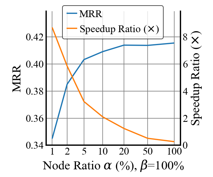
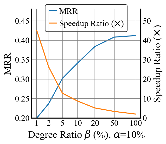
Figure 6: Performance and efficiency trade-off w.r.t. node ratio $\alpha$ and degree ratio $\beta$. Speedup ratio is relative to NBFNet.

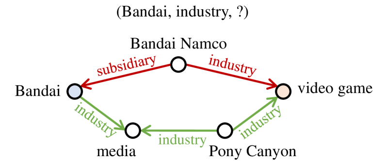
Figure 7: Visualization of important paths learned by the neural priority function in .

5 Related Work

Path-based Reasoning

Path-based methods use paths between entities for knowledge graph reasoning. Early methods like Path Ranking [28, 19] collect relational paths as symbolic features for classification. Path-RNN [31, 15] and PathCon [45] improve Path Ranking by learning the representations of paths with recurrent neural networks (RNN). However, these works operate on the full set of paths between two entities, which grows exponentially w.r.t. the path length. Typically, these methods can only be applied to paths with at most 3 edges.

To avoid the exhaustive search of paths, many methods learn to sample important paths for reasoning. DeepPath [47] and MINERVA [14] learn an agent to collect meaningful paths on the knowledge graph through reinforcement learning. These methods are hard to train due to the extremely sparse rewards. Later works improve them by engineering the reward function [29] or the search strategy [37], using multiple agents for positive and negative paths [24] or for coarse- and fine-grained paths [52]. [11] and [33] use a variational formulation to learn a sparse prior for path sampling. Another category of methods utilizes the dynamic programming to search paths in a polynomial time. NeuralLP [50] and DRUM [35] use dynamic programming to learn linear combination of logic rules. All-Paths [41] adopts a Floyd-Warshall-like algorithm to learn path representations between all pairs of entities. Recently, NBFNet [58] and RED-GNN [54] leverage a Bellman-Ford-like algorithm to learn path representations from a single-source entity to all entities. While dynamic programming methods achieve state-of-the-art results among path-based methods, they need to perform message passing on the full knowledge graph. By comparison, our learns a priority function and only explores a subset of paths, which is more scalable than existing dynamic programming methods.

Efficient Graph Neural Networks

Our work is also related to efficient graph neural networks, since both try to improve the scalability of graph neural networks (GNNs). Sampling methods [21, 9, 26, 51] reduce the cost of message passing by computing GNNs with a sampled subset of nodes and edges. Non-parametric GNNs [27, 46, 18, 10] decouple feature propagation from feature transformation, and reduce time complexity by preprocessing feature propagation. However, both sampling methods and non-parametric GNNs are designed for homogeneous graphs, and it is not straightforward to adapt them to knowledge graphs. On knowledge graphs, RS-GCN [17] learns to sample neighborhood with reinforcement learning. DPMPN [48] learns an attention to iteratively select nodes for message passing. SQALER [1] first predicts important path types based on the query, and then applies GNNs on the subgraph extracted by the predicted paths. Our shares the same goal with these methods, but learns a neural priority function to iteratively select important paths.

6 Discussion and Conclusion

Limitation and Future Work

One limitation for is that we focus on algorithm design rather than system design. As a result, the improvement in time and memory cost is much less than the improvement in the number of messages (Tab. 4.2 and App. E). In the future, we will co-design the algorithm and the system to further improve the efficiency.

Societal Impact

This work proposes a scalable model for path-based reasoning. On the positive side, it reduces the training and test time of reasoning models, which helps control carbon emission. On the negative side, reasoning models might be used in malicious activities, such as discovering sensitive relationship in anonymized data, which could be augmented by a more scalable model.

Conclusion

We propose , a scalable path-based method, to solve knowledge graph reasoning by searching for important paths, which is guided by a neural priority function. Experiments on both transductive and inductive knowledge graphs verify the performance and efficiency of . Meanwhile, is the first path-based method that scales to million-scale knowledge graphs.

Appendix A Path-based Reasoning with A* Algorithm

Here we prove the correctness of path-based reasoning with A* algorithm.

A.1 Iterative Path Selection for Computing Important Paths

First, we prove that $\hat{{\mathcal{P}}}_{u\leadsto v|q}^{(t)}$ computed by Eqn. 6 and 7 equals to the set of important paths and paths that are different from important paths in the last hop.

Theorem A.1.

If $m_{q}({\mathcal{P}}):2^{\mathcal{P}}\mapsto 2^{\mathcal{P}}$ can select all important paths from a set of paths ${\mathcal{P}}$, the set of paths $\hat{{\mathcal{P}}}_{u\leadsto v|q}^{(t)}$ computed by Eqn. 6 and 7 equals to the set of important paths and paths that are different from important paths in the last hop of length $t$.

$$\hat{{\mathcal{P}}}_{u\leadsto v|q}^{(0)}\leftarrow\{(u,\text{self loop},v)\}~{}\text{if}~{}u=v~{}\text{else}~{}\varnothing$$ (6)

$$\hat{{\mathcal{P}}}_{u\leadsto v|q}^{(t)}\leftarrow\bigcup_{\begin{subarray}{c}x\in{\mathcal{V}}\\ (x,r,v)\in{\mathcal{E}}(v)\end{subarray}}\left\{P+\{(x,r,v)\}\middle|P\in m_{q}(\hat{{\mathcal{P}}}_{u\leadsto x|q}^{(t-1)})\right\}$$ (7)

Proof.

We use ${\mathcal{Q}}_{u\leadsto v|q}^{(t)}$ to denote the set of important paths and paths that are different from important paths in the last hop of length $t$. For paths of length $0$, we define them to be important as they should be the prefix of some important paths. Therefore, ${\mathcal{Q}}_{u\leadsto v|q}^{(0)}=\{(u,\text{self loop},v)\}$ if $u=v$ else $\varnothing$. We use $P_{:-1}$ to denote the prefix of path $P$ without the last hop. The goal is to prove $\hat{{\mathcal{P}}}_{u\leadsto v|q}^{(t)}={\mathcal{Q}}_{u\leadsto v|q}^{(t)}$.

First, we prove $\hat{{\mathcal{P}}}_{u\leadsto v|q}^{(t)}\subseteq{\mathcal{Q}}_{u\leadsto v|q}^{(t)}$. It is obvious that $\hat{{\mathcal{P}}}_{u\leadsto v|q}^{(0)}\subseteq{\mathcal{Q}}_{u\leadsto v|q}^{(0)}$. In the case of $t>0$, $\forall P\in\hat{{\mathcal{P}}}_{u\leadsto v|q}^{(t)}$, we have $P_{:-1}\in m_{q}(\hat{{\mathcal{P}}}_{u\leadsto v|q}^{(t-1)})$ according to Eqn. 7. Therefore, $P\in{\mathcal{Q}}_{u\leadsto v|q}^{(t)}$.

Second, we prove ${\mathcal{Q}}_{u\leadsto v|q}^{(t)}\subseteq\hat{{\mathcal{P}}}_{u\leadsto v|q}^{(t)}$ by induction. For the base case $t=0$, it is obvious that ${\mathcal{Q}}_{u\leadsto v|q}^{(0)}\subseteq\hat{{\mathcal{P}}}_{u\leadsto v|q}^{(0)}$. For the inductive case $t>0$, $\forall Q\in{\mathcal{Q}}_{u\leadsto v|q}^{(t)}$, $Q_{:-1}$ is an important path of length $t-1$ according to the definition of ${\mathcal{Q}}_{u\leadsto v|q}^{(t)}$. $Q_{:-1}\in m_{q}({\mathcal{Q}}_{u\leadsto v|q}^{(t-1)})\subseteq{\mathcal{Q}}_{u\leadsto v|q}^{(t-1)}$ according to the definition of $m_{q}(\cdot)$ and ${\mathcal{Q}}_{u\leadsto v|q}^{(t-1)}$. Based on the inductive assumption, we get $Q_{:-1}\in\hat{{\mathcal{P}}}_{u\leadsto v|q}^{(t-1)}$. Therefore, $Q\in\hat{{\mathcal{P}}}_{u\leadsto v|q}^{(t)}$ according to Eqn. 7. ∎

As a corollary of Thm. A.1, $\hat{{\mathcal{P}}}_{u\leadsto v|q}$ is a slightly larger superset of the important paths $P_{u\leadsto v|q}$.

Corollary A.2.

If the end nodes of important paths are uniformly distributed in the knowledge graph, the expected size of $\hat{{\mathcal{P}}}_{u\leadsto v|q}^{(t)}$ is $\left|{\mathcal{P}}_{u\leadsto v|q}^{(t)}\right|+\frac{|{\mathcal{E}}|}{|{\mathcal{V}}|}\left|{\mathcal{P}}_{u\leadsto v|q}^{(t-1)}\right|$.

Proof.

Thm. A.1 indicates that $\hat{{\mathcal{P}}}_{u\leadsto v|q}^{(t)}$ contains two types of paths: important paths and paths that are different from important paths in the last hop of length $t$. The number of the first type is $\left|{\mathcal{P}}_{u\leadsto v|q}^{(t)}\right|$. Each of the second type corresponds to an important path of length $t-1$. From an inverse perspective, each important path of length $t-1$ generates $d$ paths of the second type for $\hat{{\mathcal{P}}}_{u\leadsto v|q}^{(t)}$, where $d$ is the degree of the end node in the path. If the end nodes are uniformly distributed in the knowledge graph, we have $\mathbb{E}\left[\hat{{\mathcal{P}}}_{u\leadsto v|q}^{(t)}\right]=\left|{\mathcal{P}}_{u\leadsto v|q}^{(t)}\right|+\frac{|{\mathcal{E}}|}{|{\mathcal{V}}|}\left|{\mathcal{P}}_{u\leadsto v|q}^{(t-1)}\right|$. For real-world knowledge graphs, $\frac{|{\mathcal{E}}|}{|{\mathcal{V}}|}|$ is usually a small constant (e.g., $\leq 50$), and $\left|\hat{{\mathcal{P}}}_{u\leadsto v|q}^{(t)}\right|$ is slightly larger than $\left|{\mathcal{P}}_{u\leadsto v|q}^{(t)}\right|$ in terms of complexity. ∎

A.2 From Iterative Path Selection to Iterative Node Selection

Second, we demonstrate that Eqn. 7 can be solved by Eqn. 8 if paths with the same length and the same stop node can be merged.

Proposition A.3.

If $m_{q}({\mathcal{P}})$ selects paths only based on the length $t$, the start node $u$ and the end node $x$ of each path, by replacing $m_{q}({\mathcal{P}})$ with $n_{uq}^{(t)}({\mathcal{V}})$, $\hat{{\mathcal{P}}}_{u\leadsto v|q}^{(t)}$ can be computed as follows

$$\hat{{\mathcal{P}}}_{u\leadsto v|q}^{(t)}\leftarrow\bigcup_{\begin{subarray}{c}x\in n_{uq}^{(t-1)}({\mathcal{V}})\\ (x,r,v)\in{\mathcal{E}}(v)\end{subarray}}\left\{P+\{(x,r,v)\}\middle|P\in\hat{{\mathcal{P}}}_{u\leadsto x|q}^{(t-1)}\right\}$$ (8)

This proposition is obvious. As a result of Prop. A.3, we merge paths by their length and stop nodes, which turns the exponential tree search to a polynomial dynamic programming algorithm.

A.3 Reasoning with A* Algorithm

Finally, we prove that the A* iteration (Eqn. 9) covers all important paths for reasoning (Eqn. 5).

Theorem A.4.

If $n_{uq}^{(t)}({\mathcal{V}}):2^{\mathcal{V}}\mapsto 2^{\mathcal{V}}$ can determine whether paths from $u$ to $x$ are important or not, and $\langle\oplus,\otimes\rangle$ forms a semiring [23], the representation ${\bm{h}}_{q}(u,v)$ for path-based reasoning can be computed by

$${\bm{h}}_{q}^{(t)}(u,v)\leftarrow{\bm{h}}_{q}^{(0)}(u,v)\oplus\bigoplus_{\begin{subarray}{c}x\in n_{uq}^{(t-1)}({\mathcal{V}})\\ (x,r,v)\in{\mathcal{E}}(v)\end{subarray}}{\bm{h}}_{q}^{(t-1)}(u,x)\otimes{\bm{w}}_{q}(x,r,v)$$ (9)

Proof.

In order to prove Thm. A.4, we first prove a lemma for the analytic form of ${\bm{h}}_{q}^{(t)}(u,v)$, and then show that $\lim_{t\rightarrow\infty}{{\bm{h}}_{q}^{(t)}(u,v)}$ converges to the goal of path-based reasoning.

Lemma A.5.

Under the same condition as Thm. A.4, the intermediate representation ${\bm{h}}_{q}^{(t)}(u,v)$ computed by Eqn. 2 and 9 aggregates all important paths within a length of $t$ edges, i.e.

$${\bm{h}}_{q}^{(t)}(u,v)=\bigoplus_{P\in\hat{{\mathcal{P}}}_{u\leadsto v|q}^{(\leq t)}}\bigotimes_{i=1}^{|P|}{\bm{w}}_{q}(e_{i})$$ (15)

where $\hat{{\mathcal{P}}}_{u\leadsto v|q}^{(\leq t)}=\bigcup_{k=0}^{t}\hat{{\mathcal{P}}}_{u\leadsto v|q}^{(k)}$.

Proof.

We prove Lem. A.5 by induction. Let $\scriptsize{0}⃝_{q}$ and $\scriptsize{1}⃝_{q}$ denote the identity elements of $\oplus$ and $\otimes$ respectively. We have $\text{1}_{q}(u=v)=\scriptsize{1}⃝_{q}$ if $u=v$ else $\scriptsize{0}⃝_{q}$. Note paths of length $0$ only contain self loops, and we define them as important paths, since they should be prefix of some important paths.

For the base case $t=0$, we have ${\bm{h}}_{q}^{(0)}(u,u)=\scriptsize{1}⃝_{q}=\bigoplus_{P\in{\mathcal{P}}_{u\leadsto u|q}:|P|\leq 0}\bigotimes_{i=1}^{|P|}{\bm{w}}_{q}(e_{i})$ since the only path from $u$ to $u$ is the self loop, which has the representation $\scriptsize{1}⃝_{q}$. For $u\neq v$, we have ${\bm{h}}_{q}^{(0)}(u,v)=\scriptsize{0}⃝_{q}=\bigoplus_{P\in{\mathcal{P}}_{u\leadsto v|q}:|P|\leq 0}\bigotimes_{i=1}^{|P|}{\bm{w}}_{q}(e_{i})$ since there is no important path from $u$ to $v$ within length $0$.

For the inductive case $t>0$, we have

$${\bm{h}}^{(t)}_{q}(u,v) ={\bm{h}}^{(0)}_{q}(u,v)\oplus\bigoplus_{\begin{subarray}{c}x\in n_{uq}^{(t-1)}({\mathcal{V}})\\ (x,r,v)\in{\mathcal{E}}(v)\end{subarray}}{\bm{h}}_{q}^{(t-1)}(u,x)\otimes{\bm{w}}_{q}(x,r,v)$$ (16)

$$={\bm{h}}^{(0)}_{q}(u,v)\oplus\bigoplus_{\begin{subarray}{c}x\in n_{uq}^{(t-1)}({\mathcal{V}})\\ (x,r,v)\in{\mathcal{E}}(v)\end{subarray}}\left(\bigoplus_{P\in\hat{{\mathcal{P}}}_{u\leadsto v|q}^{(\leq t-1)}}\bigotimes_{i=1}^{|P|}{\bm{w}}_{q}(e_{i})\right)\otimes{\bm{w}}_{q}(x,r,v)$$ (17)

$$={\bm{h}}^{(0)}_{q}(u,v)\oplus\bigoplus_{\begin{subarray}{c}x\in n_{uq}^{(t-1)}({\mathcal{V}})\\ (x,r,v)\in{\mathcal{E}}(v)\end{subarray}}\left[\bigoplus_{P\in\hat{{\mathcal{P}}}_{u\leadsto v|q}^{(\leq t-1)}}\left(\bigotimes_{i=1}^{|P|}{\bm{w}}_{q}(e_{i})\right)\otimes{\bm{w}}_{q}(x,r,v)\right]$$ (18)

$$=\left(\bigoplus_{P\in\hat{{\mathcal{P}}}_{u\leadsto v|q}^{(0)}}\bigotimes_{i=1}^{|P|}{\bm{w}}_{q}(e_{i})\right)\oplus\left(\bigoplus_{P\in\hat{{\mathcal{P}}}_{u\leadsto v|q}^{(\leq t)}\setminus\hat{{\mathcal{P}}}_{u\leadsto v|q}^{(0)}}\bigotimes_{i=1}^{|P|}{\bm{w}}_{q}(e_{i})\right)$$ (19)

$$=\bigoplus_{P\in\hat{{\mathcal{P}}}_{u\leadsto v|q}^{(\leq t)}}\bigotimes_{i=1}^{|P|}{\bm{w}}_{q}(e_{i}),$$ (20)

where Eqn. 17 uses the inductive assumption, Eqn. 18 relies on the distributive property of $\otimes$ over $\oplus$, and Eqn. 19 uses Prop. A.3. In the above equations, $\bigotimes$ and $\otimes$ are always applied before $\bigoplus$ and $\oplus$. ∎

Since ${\mathcal{P}}_{u\leadsto v|q}^{(t)}\subseteq\hat{{\mathcal{P}}}_{u\leadsto v|q}^{(t)}$, we have ${\mathcal{P}}_{u\leadsto v|q}\subseteq\hat{{\mathcal{P}}}_{u\leadsto v|q}\subseteq{\mathcal{P}}_{u\leadsto v}$. Based on Lem. A.5 and Eqn. 5, it is obvious to see that

$$\lim_{t\rightarrow\infty}{{\bm{h}}_{q}^{(t)}(u,v)}=\bigoplus_{P\in\hat{{\mathcal{P}}}_{u\leadsto v|q}}{\bm{h}}_{q}(P)\approx\bigoplus_{P\in{\mathcal{P}}_{u\leadsto v}}{\bm{h}}_{q}(P)={\bm{h}}_{q}(u,v)$$ (21)

Therefore, Thm. A.4 holds. ∎

Appendix B Additional Edge Selection Step in

As demonstrated in Sec. 3.2, selects top-$K$ nodes according to the current priority function, and computes the A* iteration

$${\bm{h}}_{q}^{(t)}(u,v)\leftarrow{\bm{h}}_{q}^{(0)}(u,v)\oplus\bigoplus_{\begin{subarray}{c}x\in{\mathcal{X}}^{(t)}\\ (x,r,v)\in{\mathcal{E}}(v)\end{subarray}}s_{uq}^{(t-1)}(x)\left({\bm{h}}_{q}^{(t-1)}(u,x)\otimes{\bm{w}}_{q}(x,r,v)\right)$$ (12)

However, even if we choose a small $K$, Eqn. 12 may still propagate the messages to many nodes in the knowledge graph, resulting in a high computation cost. This is because some nodes in the knowledge graph may have very large degrees, e.g., the entity Human is connected to every person in the knowledge graph. In fact, it is not necessary to propagate the messages to every neighbor of a node, especially if the node has a large degree. Based on this observation, we propose to further select top-$L$ edges from the neighborhood of ${\mathcal{X}}^{(t)}$ to create ${\mathcal{E}}^{(t)}$

$${\mathcal{E}}^{(t)}\leftarrow\textrm{TopL}(s_{uq}^{(t-1)}(v)|x\in{\mathcal{X}}^{(t)},(x,r,v)\in{\mathcal{E}}(x))$$ (22)

where each edge is picked according to the priority of node $v$, i.e., the tail node of an edge. By doing so, we reuse the neural priority function and avoid introducing any additional priority function. The intuition of Eqn. 22 is that if an edge $(x,r,v)$ goes to a node with a higher priority, it is likely we are propagating towards the answer entities. With the selected edges ${\mathcal{E}}^{(t)}$, the A* iteration becomes

$${\bm{h}}_{q}^{(t)}(u,v)\leftarrow{\bm{h}}_{q}^{(0)}(u,v)\oplus\bigoplus_{\begin{subarray}{c}x\in{\mathcal{X}}^{(t)}\\ (x,r,v)\in{\mathcal{E}}^{(t)}(v)\end{subarray}}s_{uq}^{(t-1)}(x)\left({\bm{h}}_{q}^{(t-1)}(u,x)\otimes{\bm{w}}_{q}(x,r,v)\right)$$ (23)

which is also the implementation in Alg. 1.

Appendix C Padding-Free Operations

In , different training samples may have very different sizes for the selected nodes ${\mathcal{V}}^{(t)}$ and ${\mathcal{E}}^{(t)}$. To avoid the additional computation over padding in conventional batched execution, we introduce padding-free operations, which operates on the concatenation of samples without any padding.

Specifically, padding-free operations construct IDs for each sample in the batch, such that we can distinguish different samples when we apply operations to the whole batch. As showed in Fig. 8, for padding-free topk, we pair the inputs with their sample IDs, and cast the problem as a multi-key sort over the whole batch. The multi-key sort is implemented by two calls to standard stable sort operations sequentially. We then apply indexing operations and remove the sample IDs to get the desired output. Alg. C provides the pseudo code for padding-free topk in PyTorch.

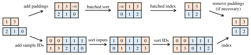
Figure 8: Comparison between padding-based topk (up) and padding-free topk (down) for $K=2$. Padding-based operations first add paddings to create a padded tensor for batched operations, and then remove the paddings. Padding-free operations pair the inputs with their sample IDs (showed in colors), and then apply single-sample operations over the whole batch.

Algorithm 2 Padding-free implementation of topk in PyTorch

Input: Input values of each sample inputs}, size of each sample \mintinlinepython

sizes,

K} \\
    \textbf

Output: TopK values of each sample, indices of topk values

⬇

# the sample id of each element

sample_ids = torch.arange(batch_size).repeat_interleave(sizes)

# multi-key sort of (sample_ids, inputs)

indices = inputs.argsort()

indices = sample_ids[indices].argsort(stable=True)

sorteds = inputs[indices]

# take top-k values of each sample

ranges = torch.arange(K).repeat(batch_size)

ranges = ranges + sizes.cumsum(0).repeat_interleave(K) - K

return sorteds[ranges], indices[ranges]

Appendix D Datasets & Evaluation

Dataset statistics for transductive and inductive knowledge graph reasoning is summarized in Tab. 7 and 8 respectively. For the transductive setting, given a query head (or tail) and a query relation, we rank each answer tail (or head) entity against all negative entities. For the inductive setting, we follow [54] and rank each each answer tail (or head) entity against all negative entities, rather than 50 randomly sampled negative entities in [39]. We report the mean reciprocal rank (MRR) and HITS at K (H@K) of the rankings.

Table 7: Dataset statistics for transductive knowledge graph reasoning.

Dataset	#Relation	#Entity	#Triplet
			#Train	#Valid	#Test
FB15k-237	237	14,541	272,115	17,535	20,466
WN18RR	11	40,943	86,835	3,034	3,134
YAGO3-10	37	123,182	1,079,040	5000	5000
ogbl-wikikg2	535	2,500,604	16,109,182	429,456	598,543

Table 8: Dataset statistics for inductive knowledge graph reasoning.

Dataset #Relation Train Validation Test #Entity #Query #Fact #Entity #Query #Fact #Entity #Query #Fact FB15k-237 v1 180 1,594 4,245 4,245 1,594 489 4,245 1,093 205 1,993 v2 200 2,608 9,739 9,739 2,608 1,166 9,739 1,660 478 4,145 v3 215 3,668 17,986 17,986 3,668 2,194 17,986 2,501 865 7,406 v4 219 4,707 27,203 27,203 4,707 3,352 27,203 3,051 1,424 11,714 WN18RR v1 9 2,746 5,410 5,410 2,746 630 5,410 922 188 1,618 v2 10 6,954 15,262 15,262 6,954 1,838 15,262 2,757 441 4,011 v3 11 12,078 25,901 25,901 12,078 3,097 25,901 5,084 605 6,327 v4 9 3,861 7,940 7,940 3,861 934 7,940 7,084 1,429 12,334

As for efficiency evaluation, we compute the number of messages (#message) per step, wall time per epoch and memory cost. The number of messages is averaged over all samples and steps

$$\#\text{message}=\mathbb{E}_{(u,q,v)\in{\mathcal{E}}}\mathbb{E}_{t}\left|{\mathcal{E}}^{(t)}\right|$$ (24)

The wall time per epoch is defined as the average time to complete a single training epoch. We measure the wall time based on 10 epochs. The memory cost is measured by the function

torch.cuda.max_memory_allocated()} in PyTorch.
\section

Implementation Details Our work is based on the open-source codebase of path-based reasoning with Bellman-Ford algorithm. Tab. 9 lists the hyperparameters for on all datasets and in both transductive and inductive settings. For the inductive setting, we use the same set of hyperparameters for all 4 splits of each dataset.

Table 9: Hyperparameter configurations of on all datasets. For FB15k-237, WN18RR and YAGO3-10, we use the same hyperparameters as NBFNet [58], except for the neural priority function introduced in . There is no publicly available hyperparameters of NBFNet on ogbl-wikikg2.

Hyperparameter FB15k-237 WN18RR YAGO3-10 ogbl-wikikg2 transductive inductive transductive inductive transductive transductive Message Passing #step ($T$) 6 6 6 6 6 6 hidden dim. 32 32 32 32 32 32 message DistMult DistMult DistMult DistMult DistMult DistMult aggregation PNA sum PNA sum PNA sum Priority Function ${\bm{g}}(\cdot)$ #layer 1 1 1 1 1 1 $f(\cdot)$ #layer 2 2 2 2 2 2 hidden dim. 64 64 64 64 64 64 node ratio $\alpha$ 10% 50% 10% 5% 10% 0.2% degree ratio $\beta$ 100% 100% 100% 100% 100% 100% Learning optimizer Adam Adam Adam Adam Adam Adam batch size 256 256 256 256 40 128 learning rate 5e-3 5e-3 5e-3 5e-3 5e-3 5e-3 #epoch 20 20 20 20 0.4 0.2 adv. temperature 0.5 0.5 1 1 0.5 0.5 #negative 32 32 32 32 32 1,048,576

Neural Parameterization

For a fair comparison with existing path-based methods, we follow NBFNet [58] and parameterize $\bigoplus$ with principal neighborhood aggregation (PNA), which is a permutation-invariant function over a set of elements. We parameterize $\bigotimes$ with the relation operation from DistMult [49], i.e., vector multiplication. Note that PNA relies on the degree information of each node to perform aggregation. We observe that PNA does not generalize well when degrees are dynamically determined by the priority function. Therefore, we precompute the degree for each node on the full graph, and use them in PNA no matter how many nodes and edges are selected by the priority function. Following NBFNet [58], we parameterize the indicator function as $\text{1}_{q}(u=v)=\text{1}(u=v){\bm{q}}$. Intuitively, this produces a boundary condition of zero vectors except for the head entity $u$, which is labeled with the query embedding $q$. For ogbl-wikikg2, instead of using a boundary condition of mostly zeros, we find it is better to incorporate distance information in the boundary condition. To this end, we use the personalized PageRank score $p_{u,v}$ from $u$ to $v$ as a soft distance metric, and parameterize the indicator function as $\text{1}_{q}(u=v)=\text{1}(u=v){\bm{q}}+\text{1}(u\neq v){\bm{p}}_{u,v}$, where ${\bm{p}}_{u,v}$ is an embedding learned based on discretized value of $p_{u,v}$.

Data Augmentation

We follow the data augmentation steps of NBFNet [58]. For each triplet $(x,r,y)$, we add an inverse triplet $(y,r^{-1},x)$ to the knowledge graph, so that can propagate in both directions. Each triplet and its inverse may have different priority and are picked independently in the edge selection step. Since test queries are always missing in the graph, we remove the edges of training queries during training to prevent the model from copying the input.

Appendix E More Experiment Results

Tab. 10(b) shows the performance and efficiency results on YAGO3-10. We observe that achieves compatible performance with NBFNet, while reducing the number of messages by 16.0$\times$. also reduces the time and memory of NBFNet by 2.5$\times$ and 2.0$\times$ respectively. Tab. 11 provides all metrics of the performance on inductive knowledge graph reasoning. It can be observed that consistently outperforms all compared methods except NBFNet. achieves competitive performance compared to NBFNet, despite the fact that reduces the number of messages, wall time and memory on both datasets and all splits (Tab. 12).

Table 10: Performance and efficiency on YAGO3-10. Results of compared methods are from [38].

(a) Performance results.

Method	YAGO3-10
	MRR	H@1	H@3	H@10
DistMult	0.34	0.24	0.38	0.54
ComplEx	0.36	0.26	0.40	0.55
RotatE	0.495	0.402	0.550	0.670
NFBNet	0.563	0.480	0.612	0.708
	0.556	0.470	0.611	0.707

(b) Efficiency results.

Method YAGO3-10 #message time memory NBFNet 2,158,080 51.3 min 26.1 GiB 134,793 20.8 min 13.1 GiB Improvement 16.0$\times$ 2.5$\times$ 2.0$\times$

Table 11: Performance on inductive knowledge graph reasoning. V1-v4 refer to the 4 standard splits.

Method v1 v2 v3 v4 MRR H@1 H@10 MRR H@1 H@10 MRR H@1 H@10 MRR H@1 H@10 FB15k-237 GraIL 0.279 0.205 0.429 0.276 0.202 0.424 0.251 0.165 0.424 0.227 0.143 0.389 NeuralLP 0.325 0.243 0.468 0.389 0.286 0.586 0.400 0.309 0.571 0.396 0.289 0.593 DRUM 0.333 0.247 0.474 0.395 0.284 0.595 0.402 0.308 0.571 0.410 0.309 0.593 NBFNet 0.422 0.335 0.574 0.514 0.421 0.685 0.476 0.384 0.637 0.453 0.360 0.627 RED-GNN 0.369 0.302 0.483 0.469 0.381 0.629 0.445 0.351 0.603 0.442 0.340 0.621 0.457 0.381 0.589 0.510 0.419 0.672 0.476 0.389 0.629 0.466 0.365 0.645 WN18RR GraIL 0.627 0.554 0.760 0.625 0.542 0.776 0.323 0.278 0.409 0.553 0.443 0.687 NeuralLP 0.649 0.592 0.772 0.635 0.575 0.749 0.361 0.304 0.476 0.628 0.583 0.706 DRUM 0.666 0.613 0.777 0.646 0.595 0.747 0.380 0.330 0.477 0.627 0.586 0.702 NBFNet 0.741 0.695 0.826 0.704 0.651 0.798 0.452 0.392 0.568 0.641 0.608 0.694 RED-GNN 0.701 0.653 0.799 0.690 0.633 0.780 0.427 0.368 0.524 0.651 0.606 0.721 0.727 0.682 0.810 0.704 0.649 0.803 0.441 0.386 0.544 0.661 0.616 0.743

Table 12: Efficiency on inductive knowledge graph reasoning. V1-v4 refer to the 4 standard splits.

Method v1 v2 v3 v4 #msg. time memory #msg. time memory #msg. time memory #msg. time memory FB15k-237 NBFNet 8,490 4.50 s 2.79 GiB 19,478 11.3 s 4.49 GiB 35,972 27.2 s 6.28 GiB 54,406 50.1 s 7.99 GiB 2,644 3.40 s 0.97 GiB 6,316 8.90 s 1.60 GiB 12,153 18.9 s 2.31 GiB 18,501 33.7 s 3.05 GiB Improvement 3.2$\times$ 1.3$\times$ 2.9$\times$ 3.1$\times$ 1.3 $\times$ 2.8$\times$ 3.0$\times$ 1.4$\times$ 2.7$\times$ 2.9$\times$ 1.5$\times$ 2.6$\times$ WN18RR NBFNet 10,820 8.80 s 1.79 GiB 30,524 30.9 s 4.48 GiB 51,802 78.6 s 7.75 GiB 7,940 13.6 s 2.49 GiB 210 2.85 s 0.11 GiB 478 8.65 s 0.26 GiB 704 13.2 s 0.41 GiB 279 4.20 s 0.14 GiB Improvement 51.8$\times$ 3.1$\times$ 16.3$\times$ 63.9$\times$ 3.6$\times$ 17.2$\times$ 73.6$\times$ 6.0$\times$ 18.9$\times$ 28.5$\times$ 3.2$\times$ 17.8$\times$

Appendix F More Visualization of Learned Important Paths

Fig. 9 visualizes learned important paths on different samples. All the samples are picked from the test set of transductive FB15k-237.

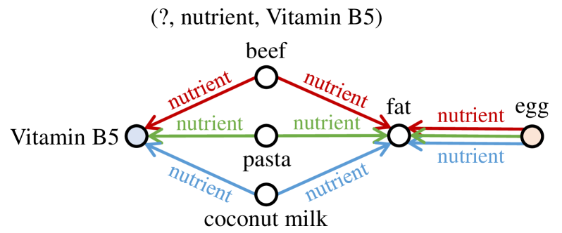
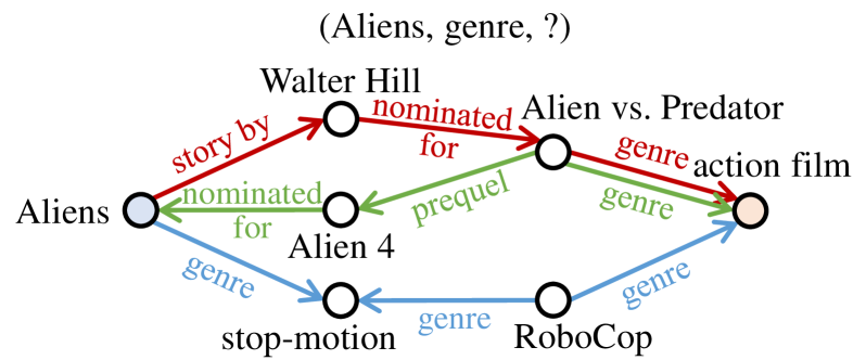
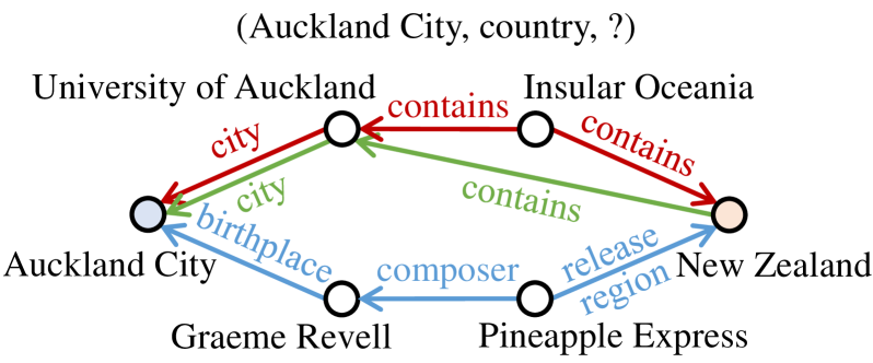
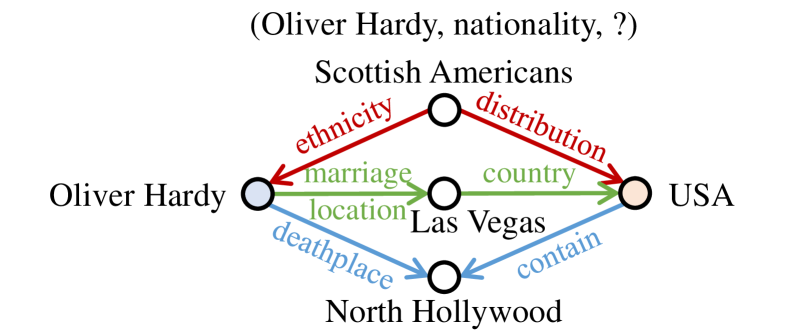
Figure 9: Visualization of important paths in on different test samples. Each important path is highlighted by a separate color.

References

- [1] Mattia Atzeni, Jasmina Bogojeska, and Andreas Loukas. Sqaler: Scaling question answering by decoupling multi-hop and logical reasoning. Advances in Neural Information Processing Systems, 34, 2021.
- [2] Sören Auer, Christian Bizer, Georgi Kobilarov, Jens Lehmann, Richard Cyganiak, and Zachary Ives. Dbpedia: A nucleus for a web of open data. In The semantic web, pages 722–735. Springer, 2007.
- [3] Yushi Bai, Zhitao Ying, Hongyu Ren, and Jure Leskovec. Modeling heterogeneous hierarchies with relation-specific hyperbolic cones. Advances in Neural Information Processing Systems, 34, 2021.
- [4] Richard Bellman. On a routing problem. Quarterly of applied mathematics, 16(1):87–90, 1958.
- [5] Jonathan Berant, Andrew Chou, Roy Frostig, and Percy Liang. Semantic parsing on freebase from question-answer pairs. In Proceedings of the 2013 conference on empirical methods in natural language processing, pages 1533–1544, 2013.
- [6] Antoine Bordes, Nicolas Usunier, Alberto Garcia-Duran, Jason Weston, and Oksana Yakhnenko. Translating embeddings for modeling multi-relational data. Advances in neural information processing systems, 26, 2013.
- [7] Ines Chami, Adva Wolf, Da-Cheng Juan, Frederic Sala, Sujith Ravi, and Christopher Ré. Low-dimensional hyperbolic knowledge graph embeddings. In Proceedings of the 58th Annual Meeting of the Association for Computational Linguistics, pages 6901–6914, 2020.
- [8] Linlin Chao, Jianshan He, Taifeng Wang, and Wei Chu. Pairre: Knowledge graph embeddings via paired relation vectors. In Proceedings of the 59th Annual Meeting of the Association for Computational Linguistics and the 11th International Joint Conference on Natural Language Processing (Volume 1: Long Papers), pages 4360–4369, 2021.
- [9] Jie Chen, Tengfei Ma, and Cao Xiao. Fastgcn: Fast learning with graph convolutional networks via importance sampling. In International Conference on Learning Representations, 2018.
- [10] Ming Chen, Zhewei Wei, Bolin Ding, Yaliang Li, Ye Yuan, Xiaoyong Du, and Ji-Rong Wen. Scalable graph neural networks via bidirectional propagation. Advances in neural information processing systems, 33:14556–14566, 2020.
- [11] Wenhu Chen, Wenhan Xiong, Xifeng Yan, and William Yang Wang. Variational knowledge graph reasoning. In Proceedings of the 2018 Conference of the North American Chapter of the Association for Computational Linguistics: Human Language Technologies, Volume 1 (Long Papers), pages 1823–1832, 2018.
- [12] Yihong Chen, Pasquale Minervini, Sebastian Riedel, and Pontus Stenetorp. Relation prediction as an auxiliary training objective for improving multi-relational graph representations. In 3rd Conference on Automated Knowledge Base Construction, 2021.
- [13] Gabriele Corso, Luca Cavalleri, Dominique Beaini, Pietro Liò, and Petar Veličković. Principal neighbourhood aggregation for graph nets. Advances in Neural Information Processing Systems, 33:13260–13271, 2020.
- [14] Rajarshi Das, Shehzaad Dhuliawala, Manzil Zaheer, Luke Vilnis, Ishan Durugkar, Akshay Krishnamurthy, Alex Smola, and Andrew McCallum. Go for a walk and arrive at the answer: Reasoning over paths in knowledge bases using reinforcement learning. In International Conference on Learning Representations, 2018.
- [15] Rajarshi Das, Arvind Neelakantan, David Belanger, and Andrew McCallum. Chains of reasoning over entities, relations, and text using recurrent neural networks. In Proceedings of the 15th Conference of the European Chapter of the Association for Computational Linguistics: Volume 1, Long Papers, pages 132–141, 2017.
- [16] Tim Dettmers, Pasquale Minervini, Pontus Stenetorp, and Sebastian Riedel. Convolutional 2d knowledge graph embeddings. In Proceedings of the AAAI conference on artificial intelligence, volume 32, 2018.
- [17] Arthur Feeney, Rishabh Gupta, Veronika Thost, Rico Angell, Gayathri Chandu, Yash Adhikari, and Tengfei Ma. Relation matters in sampling: A scalable multi-relational graph neural network for drug-drug interaction prediction. arXiv preprint arXiv:2105.13975, 2021.
- [18] Fabrizio Frasca, Emanuele Rossi, Davide Eynard, Ben Chamberlain, Michael Bronstein, and Federico Monti. Sign: Scalable inception graph neural networks. arXiv preprint arXiv:2004.11198, 2020.
- [19] Matt Gardner and Tom Mitchell. Efficient and expressive knowledge base completion using subgraph feature extraction. In Proceedings of the 2015 Conference on Empirical Methods in Natural Language Processing, pages 1488–1498, 2015.
- [20] Ben Goertzel and Cassio Pennachin. Artificial general intelligence, volume 2. Springer, 2007.
- [21] Will Hamilton, Zhitao Ying, and Jure Leskovec. Inductive representation learning on large graphs. Advances in neural information processing systems, 30, 2017.
- [22] Peter E Hart, Nils J Nilsson, and Bertram Raphael. A formal basis for the heuristic determination of minimum cost paths. IEEE transactions on Systems Science and Cybernetics, 4(2):100–107, 1968.
- [23] Udo Hebisch and Hanns Joachim Weinert. Semirings: algebraic theory and applications in computer science, volume 5. World Scientific, 1998.
- [24] Marcel Hildebrandt, Jorge Andres Quintero Serna, Yunpu Ma, Martin Ringsquandl, Mitchell Joblin, and Volker Tresp. Reasoning on knowledge graphs with debate dynamics. In Proceedings of the AAAI Conference on Artificial Intelligence, volume 34, pages 4123–4131, 2020.
- [25] Weihua Hu, Matthias Fey, Hongyu Ren, Maho Nakata, Yuxiao Dong, and Jure Leskovec. Ogb-lsc: A large-scale challenge for machine learning on graphs. arXiv preprint arXiv:2103.09430, 2021.
- [26] Wenbing Huang, Tong Zhang, Yu Rong, and Junzhou Huang. Adaptive sampling towards fast graph representation learning. Advances in neural information processing systems, 31, 2018.
- [27] Johannes Klicpera, Aleksandar Bojchevski, and Stephan Günnemann. Predict then propagate: Graph neural networks meet personalized pagerank. In International Conference on Learning Representations, 2018.
- [28] Ni Lao and William W Cohen. Relational retrieval using a combination of path-constrained random walks. Machine learning, 81(1):53–67, 2010.
- [29] Xi Victoria Lin, Richard Socher, and Caiming Xiong. Multi-hop knowledge graph reasoning with reward shaping. In EMNLP, 2018.
- [30] Farzaneh Mahdisoltani, Joanna Biega, and Fabian Suchanek. Yago3: A knowledge base from multilingual wikipedias. In 7th biennial conference on innovative data systems research. CIDR Conference, 2014.
- [31] Arvind Neelakantan, Benjamin Roth, and Andrew McCallum. Compositional vector space models for knowledge base completion. In Proceedings of the 53rd Annual Meeting of the Association for Computational Linguistics and the 7th International Joint Conference on Natural Language Processing (Volume 1: Long Papers), pages 156–166, 2015.
- [32] Judea Pearl. Probabilistic reasoning in intelligent systems: networks of plausible inference. Morgan kaufmann, 1988.
- [33] Meng Qu, Junkun Chen, Louis-Pascal Xhonneux, Yoshua Bengio, and Jian Tang. Rnnlogic: Learning logic rules for reasoning on knowledge graphs. In International Conference on Learning Representations, 2021.
- [34] Hongyu Ren, Mikhail Galkin, Michael Cochez, Zhaocheng Zhu, and Jure Leskovec. Neural graph reasoning: Complex logical query answering meets graph databases. arXiv preprint arXiv:2303.14617, 2023.
- [35] Ali Sadeghian, Mohammadreza Armandpour, Patrick Ding, and Daisy Zhe Wang. Drum: End-to-end differentiable rule mining on knowledge graphs. Advances in Neural Information Processing Systems, 32, 2019.
- [36] Michael Schlichtkrull, Thomas N Kipf, Peter Bloem, Rianne van den Berg, Ivan Titov, and Max Welling. Modeling relational data with graph convolutional networks. In European semantic web conference, pages 593–607. Springer, 2018.
- [37] Yelong Shen, Jianshu Chen, Po-Sen Huang, Yuqing Guo, and Jianfeng Gao. M-walk: Learning to walk over graphs using monte carlo tree search. Advances in Neural Information Processing Systems, 31, 2018.
- [38] Zhiqing Sun, Zhi-Hong Deng, Jian-Yun Nie, and Jian Tang. Rotate: Knowledge graph embedding by relational rotation in complex space. In International Conference on Learning Representations, 2019.
- [39] Komal Teru, Etienne Denis, and Will Hamilton. Inductive relation prediction by subgraph reasoning. In International Conference on Machine Learning, pages 9448–9457. PMLR, 2020.
- [40] Kristina Toutanova and Danqi Chen. Observed versus latent features for knowledge base and text inference. In Proceedings of the 3rd workshop on continuous vector space models and their compositionality, pages 57–66, 2015.
- [41] Kristina Toutanova, Xi Victoria Lin, Wen-tau Yih, Hoifung Poon, and Chris Quirk. Compositional learning of embeddings for relation paths in knowledge base and text. In Proceedings of the 54th Annual Meeting of the Association for Computational Linguistics (Volume 1: Long Papers), pages 1434–1444, 2016.
- [42] Théo Trouillon, Johannes Welbl, Sebastian Riedel, Éric Gaussier, and Guillaume Bouchard. Complex embeddings for simple link prediction. In International Conference on Machine Learning, pages 2071–2080. PMLR, 2016.
- [43] Shikhar Vashishth, Soumya Sanyal, Vikram Nitin, and Partha Talukdar. Composition-based multi-relational graph convolutional networks. In International Conference on Learning Representations, 2020.
- [44] Denny Vrandečić and Markus Krötzsch. Wikidata: a free collaborative knowledgebase. Communications of the ACM, 57(10):78–85, 2014.
- [45] Hongwei Wang, Hongyu Ren, and Jure Leskovec. Relational message passing for knowledge graph completion. In Proceedings of the 27th ACM SIGKDD Conference on Knowledge Discovery & Data Mining, pages 1697–1707, 2021.
- [46] Felix Wu, Amauri Souza, Tianyi Zhang, Christopher Fifty, Tao Yu, and Kilian Weinberger. Simplifying graph convolutional networks. In International conference on machine learning, pages 6861–6871. PMLR, 2019.
- [47] Wenhan Xiong, Thien Hoang, and William Yang Wang. Deeppath: A reinforcement learning method for knowledge graph reasoning. In Proceedings of the 2017 Conference on Empirical Methods in Natural Language Processing (EMNLP 2017), Copenhagen, Denmark, September 2017. ACL.
- [48] Xiaoran Xu, Wei Feng, Yunsheng Jiang, Xiaohui Xie, Zhiqing Sun, and Zhi-Hong Deng. Dynamically pruned message passing networks for large-scale knowledge graph reasoning. In International Conference on Learning Representations, 2019.
- [49] Bishan Yang, Wen-tau Yih, Xiaodong He, Jianfeng Gao, and Li Deng. Embedding entities and relations for learning and inference in knowledge bases. International Conference on Learning Representations, 2015.
- [50] Fan Yang, Zhilin Yang, and William W Cohen. Differentiable learning of logical rules for knowledge base reasoning. In Advances in Neural Information Processing Systems, pages 2316–2325, 2017.
- [51] Hanqing Zeng, Hongkuan Zhou, Ajitesh Srivastava, Rajgopal Kannan, and Viktor Prasanna. Graphsaint: Graph sampling based inductive learning method. In International Conference on Learning Representations, 2019.
- [52] Denghui Zhang, Zixuan Yuan, Hao Liu, Hui Xiong, et al. Learning to walk with dual agents for knowledge graph reasoning. In Proceedings of the AAAI Conference on Artificial Intelligence, volume 36, pages 5932–5941, 2022.
- [53] Fuzheng Zhang, Nicholas Jing Yuan, Defu Lian, Xing Xie, and Wei-Ying Ma. Collaborative knowledge base embedding for recommender systems. In Proceedings of the 22nd ACM SIGKDD international conference on knowledge discovery and data mining, pages 353–362, 2016.
- [54] Yongqi Zhang and Quanming Yao. Knowledge graph reasoning with relational digraph. In Proceedings of the ACM Web Conference 2022, pages 912–924, 2022.
- [55] Zhanqiu Zhang, Jianyu Cai, Yongdong Zhang, and Jie Wang. Learning hierarchy-aware knowledge graph embeddings for link prediction. In Proceedings of the AAAI Conference on Artificial Intelligence, volume 34, pages 3065–3072, 2020.
- [56] Da Zheng, Xiang Song, Chao Ma, Zeyuan Tan, Zihao Ye, Jin Dong, Hao Xiong, Zheng Zhang, and George Karypis. Dgl-ke: Training knowledge graph embeddings at scale. In Proceedings of the 43rd International ACM SIGIR Conference on Research and Development in Information Retrieval, pages 739–748, 2020.
- [57] Zhaocheng Zhu, Shizhen Xu, Jian Tang, and Meng Qu. Graphvite: A high-performance cpu-gpu hybrid system for node embedding. In The World Wide Web Conference, pages 2494–2504, 2019.
- [58] Zhaocheng Zhu, Zuobai Zhang, Louis-Pascal Xhonneux, and Jian Tang. Neural bellman-ford networks: A general graph neural network framework for link prediction. Advances in Neural Information Processing Systems, 34, 2021.