An approximation algorithm for random generation of capacities

Abstract

Capacities on a finite set are sets functions vanishing on the empty set and being monotonic w.r.t. inclusion. Since the set of capacities is an order polytope, the problem of randomly generating capacities amounts to generating all linear extensions of the Boolean lattice. This problem is known to be intractable even as soon as $n>5$, therefore approximate methods have been proposed, most notably one based on Markov chains. Although quite accurate, this method is time consuming. In this paper, we propose the 2-layer approximation method, which generates a subset of linear extensions, eliminating those with very low probability. We show that our method has similar performance compared to the Markov chain but is much less time consuming.

Keywords: capacity, random generation, linear extension, Markov chain

1 Introduction

Capacities, introduced by Choquet [5], are monotone set functions vanishing on the empty set. They are widely used in decision making under risk and uncertainty, multicriteria decision making, and related to many combinatorial problems in Operations Research (see [8] for a detailed account).

In the phase of determining or learning a model based on capacities, it is often important to generate randomly capacities in a uniform way. The problem appears to be surprisingly difficult, due to the monotonicity constraints, and naive methods give poor results, with extremely biased distributions for some coefficients of the capacity. The theoretical exact solution to this problem is however known, since the set of capacities on a finite set $N$ is an order polytope, associated to the Boolean lattice $(2^{N},\subseteq)$, and generating uniformly random elements in an order polytope amounts to generating all linear extensions of the the underlying poset, that is, in our case, the Boolean lattice. Unfortunately, the number of linear extensions in $(2^{N},\subseteq)$ grows tremendously with $|N|$, and is even not known beyond $|N|=7$. This obliges to resort to approximate methods. The literature has produced many such methods, among which the Markov chain approach seems to give the best results.

The aim of this paper is to propose a new approximate method, counting a limited number of linear extensions, eliminating linear extensions with very low probability. The basic idea for this is to concentrate on the two top and two bottom layers on the Boolean lattice, and to eliminate one by one maximal elements in the two top layers, and minimal elements in the two bottom layers. For this reason, the method is called 2-layer approximation method.

A second contribution of the paper is to provide two ways for measuring the performance of any method generating uniformly distributed random capacities. The first way is based on the probability distribution of the coefficients of the capacity. It is shown that if a capacity $\mu$ is uniformly generated, then the distribution of $\mu(S)$ for any $S\subseteq N$ depends only on the cardinality of $S$, and is symmetric w.r.t. the distribution of $\mu(N\setminus S)$. However, the exact form of the distribution of $\mu(S)$ seems to be very difficult to compute. A second way consists in computing the centroid of the set of generated capacities, and to verify that it is close to the theoretical centroid of the polytope of capacities. Our experiments show that our 2-layer approximation method slightly outperforms the Markov chain method, while taking much less computation time.

The paper is organized as follows. Section 2 settles the problem in its full generality, relating uniform random generation with linear extensions. Section 3 focuses on the generation of capacities and gives the state of the art. The 2-layer approximation method is developed in Section 4 in full detail. Section 5 is devoted to the measure of performance of any method of random generation of capacities.

2 Preliminaries

Let $P$ be a finite set, endowed with a partial order $\preccurlyeq$, that is, a reflexive, antisymmetric and transitive binary relation. We say that $(P,\preccurlyeq)$ is a (finite) poset. Recall that $x\in P$ is maximal if $x\preccurlyeq y$ with $y\in P$ implies $x=y$. Similarly, $x\in P$ is minimal if $y\preccurlyeq x$ with $y\in P$ implies $x=y$. We denote by $\mathsf{Max}(P,\preccurlyeq)$ and $\mathsf{Min}(P,\preccurlyeq)$ (simply $\mathsf{Max}(P),\mathsf{Min}(P)$ if there is no ambiguity) the set of maximal and minimal elements of $P$, respectively.

The order polytope [15] associated to $(P,\preccurlyeq)$, denoted by $\mathcal{O}(P)$, is the set

$$\mathcal{O}(P)=\{f:P\longrightarrow[0,1]\mid f(x)\leqslant f(y)\text{ if }x\preccurlyeq y\}.$$

It is a polytope of dimension $p:=|P|$, whose volume $V(\mathcal{O}(P))$ can be computed by the following formula [15]:

$$V(\mathcal{O}(P))=\frac{e(P)}{p!},$$ (1)

where $e(P)$ is the number of linear extensions of $(P,\preccurlyeq)$. A linear extension of $(P,\preccurlyeq)$ is a total order $\leqslant$ on $P$ which is compatible with the partial order $\preccurlyeq$ in the following sense: $x\preccurlyeq y$ implies $x\leqslant y$. It is convenient to denote a linear extension by the sequence of the elements of $P$ arranged in increasing order according to $\leqslant$: assuming $P=\{x_{1},\ldots,x_{p}\}$, the linear extension $\leqslant$ is denoted by $x_{\sigma(1)},\ldots,x_{\sigma(p)}$, with $\sigma$ a permutation on $\{1,\ldots,p\}$ and $x_{\sigma(1)}<\cdots<x_{\sigma(p)}$.

Let $N:=\{1,2,\ldots,n\}$ be a finite set of $n$ elements. A (normalized) capacity [5, 16, 8] on $N$ is a set function $\mu:2^{N}\longrightarrow[0,1]$ satisfying $\mu(\varnothing)=0$, $\mu(N)=1$ (normalization), and the property $S\subseteq T\Rightarrow\mu(S)\leqslant\mu(T)$ (monotonicity).

We denote the set of capacities on $N$ by $\mathcal{C}(N)$. From its definition, one can see that $\mathcal{C}(N)$ is an order polytope, whose underlying poset is $(2^{N}\setminus\{\varnothing,N\},\subseteq)$.

3 Random generation of capacities

3.1 Random generation and linear extensions

The problem of randomly generating capacities according to a uniform distribution amounts to picking a point in the polytope $\mathcal{C}(N)$ in a uniform way. This is made simple because $\mathcal{C}(N)$ is an order polytope. According to Stanley [15], given a poset $(P,\preccurlyeq)$ with $P=\{x_{1},\ldots,x_{p}\}$ and its associated order polytope $\mathcal{O}(P)$, each linear extension of $(P,\preccurlyeq)$ defines a region in $\mathcal{O}(P)$:

$$R_{\sigma}:=\{f\in\mathcal{O}(P)\mid 0\leqslant f(x_{\sigma(1)})\leqslant f(x_{\sigma(2)})\leqslant\cdots\leqslant f(x_{\sigma(p)})\leqslant 1\}$$

where $\sigma$ is the permutation associated to the linear extension, i.e., $x_{\sigma(1)}<\cdots<x_{\sigma(p)}$. All regions $R_{\sigma}$ are identical (up to a change of coordinates), are $p$-dimensional simplices with volume $\frac{1}{p!}$, which leads to (1). Vertices of this simplex are the $p+1$ functions given by

$$0=f(x_{\sigma(1)})=\cdots=f(x_{\sigma(k)}),\ f(x_{\sigma(k+1)})=\cdots=f(x_{\sigma(p)})=1,\quad(k=0,1,\ldots,p).$$ (2)

As a consequence, the random generation of a point in $\mathcal{O}(P)$ w.r.t. a uniform distribution amounts to uniformly selecting a linear extension, and then to uniformly selecting a point in the associated region $R_{\sigma}$. The latter step is done as follows: generate $p$ independent numbers in $[0,1]$ according to the uniform distribution, then order them in increasing order, say, $z_{1}\leqslant\cdots\leqslant z_{p}$, and put $f(x_{\sigma(1)})=z_{1},\ldots,f(x_{\sigma(p)})=z_{p}$. This define $f\in\mathcal{O}(P)$.

The above technique can be applied to the uniform generation of capacities. As explained above, $(2^{N}\setminus\{\varnothing,N\},\subseteq)$ is the underlying poset. It suffices to select randomly a linear extension $<$ of $(2^{N}\setminus\{\varnothing,N\},\subseteq)$, say

$$S_{\sigma(1)}<\cdots<S_{\sigma(2^{n}-2)},$$

and then generate independently and uniformly $2^{n}-2$ numbers in $[0,1]$, letting $\mu(S_{\sigma(i)})=z_{i}$, where $z_{i}$ is the $i$th smallest generated number. The problem is then theoretically solved but the above method reveals to be intractable as soon as $n\geqslant 5$. Indeed, the number of linear extensions on the Boolean lattice $(2^{N},\subseteq)$ (note that it is equal to the number of linear extensions on $(2^{N}\setminus\{\varnothing,N\},\subseteq)$) increases extremely fast, as indicated in Table 1 below.

$n$	$e(2^{N})$
1	1
2	2
3	48
4	1680384
5	14807804035657359360
6	141377911697227887117195970316200795630205476957716480

Table 1: Number of linear extensions of $2^{N}$

There is no known closed-form formula for computing the number of linear extensions on $2^{N}$, nor is it known beyond $n=7$ (it is sequence A046873 in the Online Encyclopedia of Integer Sequences), however bounds are known (see, e.g., [2]). More generally, the problem of counting the number of linear extensions on a poset is a $\sharp$-P complete problem, as shown in [3].

As a consequence, only approximate methods can be used to generate capacities in a uniform way.

3.2 Related literature

We give here a brief account of the literature on approximate methods for generating capacities. One of the simplest method (shown in [9]) is to select randomly in each step one element of a capacity and then draw uniformly a number within an interval imposed by the monotonicity constraints of the already drawn numbers. This method, called raandom node generator, although very simple to implement, yields fairly biased results.

Several methods try to generate linear extensions of the considered poset, from which it is immediate to generate a capacity as we explained above. Karzanov and Khachiyan [10] propose to use the Markov Chain technique to generate linear extensions of a given poset $P$. Consider each linear extension as a state of a Markov Chain, and denote by $E$ the set of all linear extensions of $P$. The Markov chain with its transition probability matrix describes a random walk through the simplices of the order polytope $\mathcal{O}(P)$, and Karzanov and Khachiyan prove that its transition probability is an ergodic time-reversible Markov chain with a uniform stationary distribution, which means that for an arbitrary initial probability distribution on $E$, after $T$ steps ($T$ large enough), the distribution converges to the uniform distribution on $E$. Thus, for any given poset $P$ and sufficiently large $T$, the Markov chain method gives a nearly uniform generator of linear extensions of the poset. However, when the cardinality of $P$ is large, it is costly in computation time. In addition to the original classical Karzanov-Khachiyan chain method, there exist some more efficient Markov Chain algorithms, for example, Bubley and Dyer introduced the Insertion Chain algorithm in [4], while [17] mentions some other Markov Chain algorithms.

Combarro et al. [6] gives a good survey of methods of generating capacities, and propose a method to generate linear extensions of $P$, which consists in selecting a minimal element of $P$ with a certain probability, then delete it and repeat this procedure until all elements have been selected. If we could determine this probability exactly, we would obtain an exact method. For example, for generating 2-symmetric capacities, Miranda and Garcia Segador [13] transform the problem into generating a linear extension of the Young rectangular diagram. Since there exists a closed-form formula for the number of linear extensions of the Young diagram, according to the general probability formula of an element $x$ being selected $\mathbb{P}(x)=\frac{e(P\setminus x)}{e(P)}$ (see Formula (3) below), we get an exact method to generate 2-symmetric capacities. Besides, Beliakov introduces an approximation method in [1] to generate supermodular capacities, and Miranda and Garcia Segador introduce an exact method in [14] to generate 2-additive capacities.

For a general capacity, the idea of generating a linear extension by the method introduced in [6] could be used, at the condition to find a way to determine the probability of selecting an element. Miranda and Garcia Segador have proposed some approximation methods to obtain this probability, namely the Bottom-up method [12], while Combarro et al. have proposed the Minimals Plus method [7].

In this article, we present another approximation method to determine the probability of selecting a minimal (or maximal) element, which is presented in the next section.

4 The 2-layer approximation algorithm

4.1 Basic idea

Let us consider an arbitrary poset $(P,\preccurlyeq)$ with $P=\{x_{1},\ldots,x_{p}\}$. Clearly, any linear extension $x_{\sigma(1)},\ldots,x_{\sigma(p)}$ starts with a minimal element and terminates with a maximal element, i.e., $x_{\sigma(1)}\in\mathsf{Min}(P)$ and $x_{\sigma(p)}\in\mathsf{Max}(P)$. Observe that $x_{\sigma(2)}$ must be a minimal element of $P\setminus\{x_{\sigma(1)}\}$, and $x_{\sigma(p-1)}$ is a maximal element on $P\setminus\{x_{\sigma(p)}\}$, and so on. This gives a recursive structure to linear extensions.

Based on this observation, the probability that a linear extension of $P$ starts with $m\in\mathsf{Min}(P)$ is

$$\mathrm{Pr}(m\mid P) =\frac{e(P\setminus\{m\})}{e(P)}$$

$$=1-\frac{\sum_{m^{\prime}\in\mathsf{Min}(P),m^{\prime}\neq m}e(P\setminus\{m^{\prime}\})}{e(P)},$$ (3)

and smilarly the probability that a linear extension terminates with $M\in\mathsf{Max}(P)$ is

$$\mathrm{Pr}(M\mid P) =\frac{e(P\setminus\{M\})}{e(P)}$$

$$=1-\frac{\sum_{M^{\prime}\in\mathsf{Max}(P),M^{\prime}\neq M}e(P\setminus\{M^{\prime}\})}{e(P)}.$$ (4)

Then, generating a linear extension amounts to choosing, according to the correct probability given by (3) and (4), a minimal or a maximal element of a poset which is diminished by one element at each step. As the computation of the probability directly depends on the number of linear extensions, the computation can be exact only when $P$ becomes small enough. Otherwise, some approximation must be done. The idea we propose is to take the lower part of the poset for choosing minimal elements, and the upper part for choosing maximal elements, thus neglecting minimal and maximal elements which are outside these two subparts. These two subposets are also used to make the computation of the respective probabilities by (3) and (4). The method, explained in the next subsection, is however specific to posets being subsets of the Boolean lattice $(2^{N},\subseteq)$.

4.2 Approximation method

From now on, we deal with posets which are particular subsets of $(2^{N}\setminus\{\varnothing,N\},\subseteq)$. As explained in Section 4.1, we proceed by deleting step by step minimal or maximal elements of the Boolean lattice $(2^{N}\setminus\{\varnothing,N\},\subseteq)$, which yields at each step of the process a poset $(H,\subseteq)$ which is a subset of $(2^{N}\setminus\{\varnothing,N\},\subseteq)$. For commodity, and referring to its Hasse diagram, we call nodes the subsets of $N$ in $H$, denoting them most often by $x,y,\ldots$ (unless the usual set notation $S,T,\ldots$ is more adequate), and we define a layer of $H$ as the set of all nodes (subsets) of same cardinality.

The principle of the method is to limit the search of maximal elements (resp., minimal elements) of $H$ as well as the computation of their probability of occurrence to the two top layers (resp., to the two bottom layers). We denote by $T_{H}$ the poset formed by the two top layers of $H$, and for ease of readability often write $T_{H}[h,k,|I|]$ to specify its basic parameters $h,k,|I|$ explained below. The upper layer contains $h$ nodes of cardinality say $\ell$, with $2\leqslant\ell\leqslant n-1$, while the lower layer contains $k$ nodes of cardinality $\ell-1$, among which some of them are isolated, i.e., with no predecessor, and we denote by $I$ the set of isolated nodes and by $|I|$ its number. A node $y$ of the lower layer has predecessors in the upper layer, i.e., sets $x$ satisfying $x\supset y$. We denote by $\mathsf{prec}(y)$ the set of predecessors of $y$. Similarly, for a node $x$ of the upper layer, we denote by $\mathsf{succ}(x)$ the set of its successors, i.e., subsets of $x$ in the lower layer. In a dual way, we introduce $B_{H}$ (denoted also $B_{H}[h^{\prime},k^{\prime},|I^{\prime}|]$), the poset of the two bottom layers of $H$, with $h^{\prime}$ nodes on the upper level, $k^{\prime}$ nodes on the lower level, and $I^{\prime}$ is the set of isolated nodes in the upper (!) level. Fig. 1 illustrates the definitions.

Figure 1: Example of poset $H$ with the poset $T_{H}(2,6,1)$ formed by the two top layers framed in red. Braces and commas are omitted for denoting sets. Maximal elements of $H$ are in red. 13 is the only isolated node.

Consider $H\subseteq 2^{N}\setminus\{\varnothing,N\}$ and take a maximal element $M$ of $H$ belonging to $T_{H}$ (i.e., a maximal element of $T_{H}$), and a minimal element $m$ of $H$ belonging to $B_{H}$ (note that it is equivalent to write $T_{H}\setminus\{M\}$ or $T_{H\setminus\{M\}}$). The probabilities that $M$ and $m$ are terminal and initial elements of a linear extension of $H$ are approximated by:

$$\mathrm{Pr}(M\mid H)\approx \frac{e(T_{H}\setminus\{M\})}{e(T_{H})}=\mathrm{Pr}(M\mid T_{H})$$ (5)

$$\mathrm{Pr}(m\mid H)\approx \frac{e(B_{H}\setminus\{m\})}{e(B_{H})}=\mathrm{Pr}(m\mid B_{H}).$$ (6)

This approximation is based on the following observation: the number of nodes which are above a given node in layer $k$ increases very fast with $k$. Indeed, supposing that a node has in average $\ell$ predecessors, each predecessor has in turn $\ell$ predecessors as well, so that the number of nodes above a given one in the two layers above it is of the order $\ell^{2}$, and so on. Consequently, a node $x$ in the third layer (or below) has very little probability to become a maximal element and hence to be selected, since all nodes above it must be eliminated first, without eliminating all nodes of the 1st layer, because otherwise $x$ becomes a node of the 2nd layer.

The algorithm for the generation of linear extensions with uniform probability is described below.

generate-linext$(P,l)$
Input: a poset $P$ subset of $2^{N}\setminus\{\varnothing,N\}$
Output: a linear extension $l$ of $P$ generated with a uniform distribution
$H\leftarrow P$; $lmin\leftarrow\varnothing$; $lmax\leftarrow\varnothing$
While height of $H>2$ do
          Compute the basic parameters of $T_{H}$: $k,h,|I|$
          Select $M\in T_{H}[h,k,|I|]$ with probability $\mathrm{Pr}(M\mid T_{H}[h,k,|I|])$
          Add $M$ at the beginning of $lmax$
          Compute the basic parameters of $B_{H}$: $k^{\prime},h^{\prime},|I^{\prime}|$
          Select $m\in B_{H}[h^{\prime},k^{\prime},|I^{\prime}|]$ with probability $\mathrm{Pr}(m\mid B_{H}[h^{\prime},k^{\prime},|I^{\prime}|])$
          Add $m$ at the end of $lmin$
$H\leftarrow H\setminus\{M,m\}$
end while
% Now $H$ is reduced to two layers: $B_{H}$ and $T_{H}$ coincide
While height of $H=2$ do
         If number of nodes in the upper layer $\leqslant$ number of nodes in the lower layer then
                  Select $M\in T_{H}[h,k,|I|]$ with probability $\mathrm{Pr}(M\mid T_{H}[h,k,|I|])$
                  Add $M$ at the beginning of $lmax$
         otherwise
                  Select $m\in B_{H}[h^{\prime},k^{\prime},|I^{\prime}|]$ with probability $\mathrm{Pr}(m\mid B_{H}[h^{\prime},k^{\prime},|I^{\prime}|])$
                  Add $m$ at the end of $lmin$
          end if
end while
% Now $H$ is reduced to one layer, which is an antichain whose elements have
% the same probability
While $H\neq\varnothing$ do
          Select uniformly at random an element $x\in H$
          Add $x$ at the end of $lmin$
          $H\leftarrow H\setminus\{x\}$
end while
$l\leftarrow lmin$ ; concatenate $lmax$ to the end of $l$

Observe the particularity when the height of $H$ is equal to 2. Indeed, the two top layers coincide with the two bottom layers, so that one may either select maximal or minimal elements. In order to minimize the number of steps, $H$ is considered as $B_{H}$ if there are more nodes in the upper layer, and as $T_{H}$ otherwise.

We now aim at getting an explicit expression of $\mathrm{Pr}(M\mid T_{H}[h,k,|I|])$ (the same development can be done in a dual way for $\mathrm{Pr}(\mid B_{H}[h^{\prime},k^{\prime},|I^{\prime}|])$).

We start with a simple property and observation.

Lemma 1.

For any poset $H\subseteq 2^{N}\setminus\{\varnothing,N\}$, the number of linear extensions in the poset $T_{H}[h,k,|I|]$ is

$$e(T_{H}(h,k,|I|))=e(T_{H\setminus I}[h,k-|I|,0])\times\prod_{i=1}^{|I|}(k-|I|+h+i).$$

Proof.

Take $H\subseteq 2^{N}\setminus\{\varnothing,N\}$ and consider the two top layers $T_{H}[h,k,|I|]$. The isolated nodes being incomparable with the remaining elements, they can appear at any position in a linear extension of $T_{H}[h,k,|I|]$. Hence, there are $k+h-|I|+1$ possibilities to insert one isolated node into a linear extension of $T_{H\setminus I}[h,k-|I|,0]$, then $k+h-|I|+2$ possibilities to insert a second one independently of the first choice, etc. This yields the desired formula. ∎

Deriving other properties of $e(T_{H})$ requires some assumption on the structure of $T_{H}$. The following definition is central in our development.

Definition 1.

Let $x$ be a node of the upper layer of $T_{H}$.

1. The function $f_{x}$ assigns to every node $y$ of the lower layer an integer as follows:

   $$f_{x}(y)=\begin{cases}|\mathsf{prec}(y)|,&y\in\mathsf{succ}(x)\\ 0,&\text{otherwise.}\end{cases}$$

2. The function $n_{x}:\mathbb{N}\rightarrow\mathbb{N}$ is defined from $f_{x}$ as follows: $n_{x}(r)$ is the number of occurences of $f_{x}(y)=r$, i.e., $n_{x}(r)=|f_{x}^{-1}(r)|$. When $r>0$, it is the number of successors of $x$ having $r$ predecessors, otherwise when $r=0$ it is the number of nodes in the lower layer which are not successors of $x$.

Definitions for $B_{H}$ are dual: $x$ is in the lower layer and for every $y$ in the upper layer $f_{x}(y)$ is the number of successors of $y$, etc.

Definition 2.

We say that $T_{H}$ (respectively, $B_{H}$) is regular if $n_{x}$ is invariant with $x$, i.e., $n_{x}(r)=n_{x^{\prime}}(r)$ for every $r$ and every two nodes $x,x^{\prime}$ in the upper layer (respectively, in the lower layer).

As regularity will be the key property in the sequel, we elaborate on it and relate it to more intuitive properties. The first one is based on the following observation.

Observation 1.

For any two nodes $x,x^{\prime}$ in the upper level of poset $T_{H}$, we always have $|\mathsf{succ}(x)\cap\mathsf{succ}(x^{\prime})|\leqslant 1$.

Proof.

let $x$ be in the upper layer of $T_{H}$ and suppose that $x$ has at least two successors. As successors of $x$ have one less element than $x$, two successors of $x$ have the form $S\cup\{i\}$ and $S\cup\{j\}$, with $x=S\cup\{i,j\}$. Consequently, $S\cup\{i\}$ and $S\cup\{j\}$ cannot be successors of another node $x^{\prime}$ of the supper layer of $T_{H}$, hence $|\mathsf{succ}(x)\cap\mathsf{succ}(x^{\prime})|\leqslant 1$. ∎

We say that $T_{H}$ is closed under intersection if for every two nodes $x,x^{\prime}$ of the upper layer, $|\mathsf{succ}(x)\cap\mathsf{succ}(x^{\prime})|=1$. i.e., $x\cap x^{\prime}$ belongs to the lower layer. Similarly for the two bottom layers, $B_{H}$ is closed under union if for every node $x,x^{\prime}$ of the lower layer, $x\cup x^{\prime}$ belongs to the upper layer. See the Appendix for a characterization of posets closed under intersection.

In addition, we say that $T_{H}$ is balanced if $|\mathsf{succ}(x)|=|\mathsf{succ}(x^{\prime})|$ for every $x,x^{\prime}$ in the upper layer. Similarly, $B_{H}$ is balanced if $|\mathsf{prec}(x)|=|\mathsf{prec}(x^{\prime})|$ for every $x,x^{\prime}$ in the lower layer.

The next proposition relates all these properties.

Proposition 1.

Consider a poset $H$.

1. If $T_{H}$ is regular, then it is balanced.

2. If $T_{H}$ is closed under intersection and balanced, then it is regular.

3. Regularity of $T_{H}$ does not imply that $T_{H}$ is closed under intersection.

4. $T_{H}$ is regular if $H=2^{N}\setminus\{N,\varnothing\}$.

The same assertions hold for $B_{H}$.

(see proof in the Appendix)

Thus, in the algorithm generate-linext, the alternance of selecting maximal elements and minimal elements permits to keep as long as possible the assumption of regularity.

We are now in position to show the next important result.

Proposition 2.

Consider a poset $H$ with its two top layers $T_{H}[h,k,0]$ without isolated nodes, and suppose that it is regular. Then, for every $x$ in the upper layer,

$$e(T_{H}[h,k,0])=h\times e(T_{H\setminus\{x\}}[h-1,k,|I|]),$$ (7)

where $I$ is the set of isolated nodes in the two upper layers of $H\setminus\{x\}$.

Proof.

If $n_{x}$ is invariant w.r.t $x$, it means that every node $x$ has the same structure of successors, implying that $H\setminus\{x\}$ has a number $I$ of isolated nodes which does not depend of $x$, which in turn implies that $e(T_{H\setminus\{x\}}[h-1,k,|I|])$ does not depend on $x$. As any node of the upper layer is a maximal element, i.e., can be the last element in a linear extension, this proves (7). ∎

The next step is to establish the probability to select a maximal element from $T_{H}$. A maximal element can be either a node from the upper layer, or an isolated node of the lower layer. It is easy to see that in the latter case, the probability does not depend on the isolated element. This is because an isolated node can appear in any position of the linear extension, without constraint. Interestingly, one can prove that under regularity, the same property holds for nodes of the upper layer.

Proposition 3.

Consider a poset $H$ with its two top layers $T_{H}$, and suppose that it is regular. Then, for every node $x$ of the upper layer in $T_{H}$, the probability $\mathrm{Pr}(x\mid T_{H})$ that a linear extension in $T_{H}$ terminates by $x$ is independent of $x$.

Proof.

We just need to prove that the poset $T_{H}$ is symmetric w.r.t. the nodes in the upper layer, that is, all nodes in the upper layer have the same number of successors having exactly $r$ predecessors (for any $r$). But this means that $n_{x}$ is invariant. ∎

Remark that the same property when removing a node from the bottom layer holds for the two bottom layers, with symmetric conditions.

As a consequence of the above proposition and remark, we can get an explicit expression of these probabilities.

Proposition 4.

Consider the poset $T_{H}[h,k,|I|]$ and suppose that it is regular. Then the probabilities $\mathbb{P}_{u}(T_{H}[h,k,|I|])$ that node $x$ of the upper layer terminates a linear extension, and $\mathbb{P}_{l}(T_{H}[h,k,|I|])$ that isolated node $y$ of the lower layer terminates a linear extension are given by

$$\mathbb{P}_{u}(T_{H}[h,k,|I|]) =\frac{1}{h}\frac{\prod_{i=1}^{|I^{\prime}|}(h-1+k-|I^{\prime}|+i)}{\prod_{i=1}^{|I^{\prime}|}(h-1+k-|I^{\prime}|+i)+|I|\times\prod_{i=1}^{|I^{\prime\prime}|}(h-1+k-|I^{\prime}|+i)\prod_{i=1}^{|I|-1}(h+k-|I|+i)}$$ (8)

$$\mathbb{P}_{l}(T_{H}[h,k,|I|]) =\frac{\prod_{i=1}^{|I^{\prime\prime}|}(h-1+k-|I^{\prime}|+i)\prod_{i=1}^{|I|-1}(h+k-|I|+i)}{\prod_{i=1}^{|I^{\prime}|}(h-1+k-|I^{\prime}|+i)+|I|\times\prod_{i=1}^{|I^{\prime\prime}|}(h-1+k-|I^{\prime}|+i)\prod_{i=1}^{|I|-1}(h+k-|I|+i)},$$ (9)

where $I^{\prime}$ is the set of isolated nodes in the poset $T_{H\setminus\{x\}}$, and $I\cup I^{\prime\prime}=I^{\prime}$.

Proof.

Removing a node $x$ of the upper layer of $T_{H}[h,k,|I|]$ yields the poset $T_{H\setminus\{x\}}[h-1,k,|I^{\prime}|]$ with $I^{\prime}\supseteq I$. Then by Lemma 1

$$e(T_{H\setminus\{x\}}[h-1,k,|I^{\prime}|])=e(T_{H\setminus(\{x\}\cup I^{\prime})}[h-1,k-|I^{\prime}|,0])\times\prod_{i=1}^{|I^{\prime}|}(h-1+k-|I^{\prime}|+i).$$ (10)

Removing an isolated node $y$ of the lower layer yields the poset $T_{H\setminus\{y\}}[h,k-1,|I|-1]$. Removing all isolated nodes and one node $x$ of the upper layer yields the poset $T_{H\setminus(I\cup\{x\})}[h-1,k-|I|,|I^{\prime\prime}|]$, with the disjoint union $I\cup I^{\prime\prime}=I^{\prime}$, i.e., $|I|+|I^{\prime\prime}|=|I^{\prime}|$. Applying again Lemma 1 we obtain

$$e(T_{H\setminus\{y\}}[h,k-1,|I|-1] =e(T_{H\setminus I}[h,k-|I|,0]\prod_{i=1}^{|I|-1}(h+k-|I|+i)$$

$$=h\times e(T_{H\setminus(I\cup\{x\})}[h-1,k-|I|,|I^{\prime\prime}|]\prod_{i=1}^{|I|-1}(h+k-|I|+i)$$

$$=h\times e(T_{H\setminus(I^{\prime}\cup\{x\})}[h-1,k-|I^{\prime}|,0]\prod_{i=1}^{|I^{\prime\prime}|}(h-1+k-|I^{\prime}|+i)\prod_{i=1}^{|I|-1}(h+k-|I|+i)$$ (11)

where in the second equality we have used the fact that $T_{H\setminus I}[h,k-|I|,0]$ is regular, as well as Proposition 2.

By (4), we have for any node $x$ of the upper level and any isolated node $y$:

$$\mathbb{P}_{u}(T_{H}[h,k,|I|]) =\frac{e(T_{H\setminus\{x\}}[h-1,k,|I^{\prime}|])}{e(T_{H}[h,k,|I|])}$$

$$=\frac{e(T_{H\setminus\{x\}}[h-1,k,|I^{\prime}|])}{h\times e(T_{H\setminus\{x\}}[h-1,k,|I^{\prime}|])+|I|\times e(T_{H\setminus\{y\}}[h,k-1,|I|-1])}$$

$$=\frac{1}{h}\frac{\prod_{i=1}^{|I^{\prime}|}(h-1+k-|I^{\prime}|+i)}{\prod_{i=1}^{|I^{\prime}|}(h-1+k-|I^{\prime}|+i)+|I|\times\prod_{i=1}^{|I^{\prime\prime}|}(h-1+k-|I^{\prime}|+i)\prod_{i=1}^{|I|-1}(h+k-|I|+i)}$$

where in the second equality we have used Proposition 3, and in the third equality Eqs. (10) and (11). Similarly, we get

$$\mathbb{P}_{l}(T_{H}[h,k,|I|]) =\frac{e(T_{H\setminus\{y\}}[h,k-1,|I|-1])}{h\times e(T_{H\setminus\{x\}}[h-1,k,|I^{\prime}|])+|I|\times e(T_{H\setminus\{y\}}[h,k-1,|I|-1])}$$

$$=\frac{\prod_{i=1}^{|I^{\prime\prime}|}(h-1+k-|I^{\prime}|+i)\prod_{i=1}^{|I|-1}(h+k-|I|+i)}{\prod_{i=1}^{|I^{\prime}|}(h-1+k-|I^{\prime}|+i)+|I|\times\prod_{i=1}^{|I^{\prime\prime}|}(h-1+k-|I^{\prime}|+i)\prod_{i=1}^{|I|-1}(h+k-|I|+i)}.$$

∎

As a conclusion,

$$\mathrm{Pr}(M\mid T_{H}[h,k,|I|])=\begin{cases}\mathbb{P}_{u}(T_{H}[h,k,|I|]),&\text{ if }M\text{ is a node of the upper layer}\\ \mathbb{P}_{l}(T_{H}[h,k,|I|]),&\text{ if }M\text{ is an isolated node of the lower layer.}\end{cases}$$ (12)

Similar expressions can be obtained for $\mathrm{Pr}(m\mid B_{H}(h^{\prime},k^{\prime},|I^{\prime}|))$. Both can be used in Algorithm generate-linext. Note that these expressions of probabilities are approximative, as the assumption that both $T_{H}(h,k,|I|)$ and $B_{H}(h^{\prime},k^{\prime},|I^{\prime}|)$ are regular are valid in the first iteration, but not necessarily in the subsequent iterations.

4.3 Example

We illustrate the 2-layer approximation algorithm by applying it for generating a linear extension with $n=4$ (see Figure 2 (a), (b), … (i)). For simplicity, sets are denoted by 123 instead of $\{1,2,3\}$, etc.

1. (a): the two top layers are considered. Here, since all maximal nodes are on the first layer, by Proposition 3, all maximal nodes have the same probability of 0.25. Suppose 234 is selected, which yields Figure (b).

2. (b): now the two bottom layers are considered. Similarly, all minimal nodes are equiprobable. Suppose node 1 is selected, this yields (c).

3. (c): As for (a), we consider again the two top layers. All maximal nodes are on the first layer, hence equiprobable. Supposing 134 is selected, (d) is obtained.

4. (d): As for (b), we consider the two bottom layers, whose minimal nodes are on the bottom layer, hence equiprobable. Supposing node 4 is selected, we obtain (e).

5. (e): In the two upper layers, one maximal node is on the second layer. Then Proposition 4 has to be used to compute the probabilities for the first and second layer, which are respectively 0.437 and 0.125. Supposing 124 is selected, (f) is obtained.

6. (f): In the two bottom layers, one minimal element is 14 on the second layer, hence again Proposition 4 must be used. One finds 0.437 for nodes 2 and 3, and 0.125 for 14. Supposing 14 is selected, we obtain (g).

7. (g): Now the probability of selecting 123 is 0.67, and is 0.167 for selecting 24 and 34. Supposing 123 is selected, we obtain (h).

8. (h): The two top and bottom layers coincide. We consider them as the two bottom layers, since there are less minimal elements than maximal elements, and select a minimal element. They are equiprobable. Supposing node 2 is selected, (i) is obtained.

9. (i): Again, we select a minimal node. Applying Proposition 4, the probabilities are 0.67 for selecting node 3, and 0.167 for selecting 12 and 24. Supposing node 3 is selected, we obtain (j).

10. (j): there is only one layer, i.e., all nodes are both maximal and minimal and are equiprobable. We may suppose that they are selected in this order: 12, 34, 24, 23, 13.

Finally, the obtained linear extension is: 1, 4, 14, 2, 3, 12, 34, 24, 23, 13, 123, 124, 134, 234.

Figure 2: Process of node selection according to Algorithm generate-linext. The dotted red and green boxes indicate the two top and bottom layers under consideration, respectively. Red nodes are maximal elements in the two top layers, while green nodes are minimal elements in the two bottom layers.

5 Measures of performance

An important point is to be able to assess the performance of a given algorithm generating capacities in a uniform way, i.e., how much uniform is the distribution obtained? Given the high dimension of the polyhedron of capacities, no graphical view is possible, and the topic appears to be more difficult than it looks at first sight. In what follows, we propose two ways of measuring the performance, based on the distribution of $\mu(S)$ for a given subset $S$, and on the centroid of $\mathcal{C}(N)$.

5.1 Distribution of $\mu(S)$

Uniform distribution of the capacity does not mean that the distribution of $\mu(S)$ for any $S\subseteq N$, $S\neq\varnothing,N$ is uniform. An explicit and convenient expression for the distribution of $\mu(S)$ seems however very difficult to obtain. The following can be said, however.

We denote by $\boldsymbol{\mu}$ the corresponding random variable. Refering to the notation of Section 3.1, consider a linear extension associated to the permutation $\sigma$ on $2^{N}\setminus\{\varnothing,N\}$, and $R_{\sigma}$ the corresponding simplex in $\mathcal{C}(N)$. Supposing $\boldsymbol{\mu}\in R_{\sigma}$, we have that $\boldsymbol{\mu}(S_{\sigma(k)})$ follows the distribution of the $k$th order statistics on $[0,1]$. It is known that the probability density function $f_{(k)}$ of the $k$th order statistics on $[0,1]$ when the underlying $2^{n}-2$ random variables are i.i.d. and uniform is a Beta distribution:

$$f_{(k)}(u)=(2^{n}-2)\binom{2^{n}-3}{k-1}(1-u)^{2^{n}-2-k}u^{k-1}=\mathrm{Beta}(k,2^{n}+k-1)$$

with $\mathrm{Beta}(r,s)=\frac{1}{B(r,s)}u^{r-1}(1-u)^{s-1}$, and $B(r,s)$ is the Beta function

$$B(r,s)=\int_{0}^{1}t^{r-1}(1-t)^{s-1}\mathrm{d}t=\frac{\Gamma(s)\Gamma(r)}{\Gamma(r+s)}$$

with $\Gamma(r)=\int_{0}^{1}t^{r-1}e^{-t}\mathrm{d}t$ the Gamma function. Denoting by $\mathrm{OS}_{k}$ the corresponding cumulative distribution function, it follows that for any $S\in 2^{N}\setminus\{\varnothing,N\}$, the distribution $F_{\boldsymbol{\mu}(S)}(\alpha)$ is given by

$$F_{\boldsymbol{\mu}(S)}(\alpha) =\mathrm{Pr}(\boldsymbol{\mu}(S)\leqslant\alpha)=\sum_{\sigma\in E(2^{N}\setminus\{\varnothing,N\})}\mathrm{Pr}(\boldsymbol{\mu}(S)\leqslant\alpha\mid\boldsymbol{\mu}\in R_{\sigma})\mathrm{Pr}(\boldsymbol{\mu}\in R_{\sigma})$$

$$=\frac{1}{e(2^{N})}\sum_{\sigma\in E(2^{N}\setminus\{\varnothing,N\})}\mathrm{Pr}(\boldsymbol{\mu}(S)\leqslant\alpha\mid\boldsymbol{\mu}\in R_{\sigma})$$

$$=\frac{1}{e(2^{N})}\sum_{\sigma\in E(2^{N}\setminus\{\varnothing,N\})}\mathrm{OS}_{k(S,\sigma)}(\alpha),$$ (13)

where $E(2^{N}\setminus\{\varnothing,N\})$ is the set of permutations corresponding to linear extensions, and $k(S,\sigma)$ is such that $S=S_{\sigma(k)}$.

Based on this formula, the following can be shown.

Lemma 2.

Assume $\boldsymbol{\mu}$ is uniformly distributed and take $\varnothing\neq S,S^{\prime}\subset N$. Then

1. $\boldsymbol{\mu}(S)$ and $\boldsymbol{\mu}(S^{\prime})$ for $|S|=|S^{\prime}|$ are identically distributed.

2. $\boldsymbol{\mu}(S)$ and $1-\boldsymbol{\mu}(N\setminus S)$ are identically distributed.

Proof.

(i) Consider distinct subsets $S,S^{\prime}\in 2^{N}\setminus\{\varnothing,N\}$ such that $|S|=|S^{\prime}|$, and fix a linear extension $\sigma$. Then there exists a permutation $\pi$ on $N$ such that $\pi(S)=S^{\prime}$, and $k(S,\sigma)=k(\pi(S),\pi(\sigma))$, where $\pi(S)=\{\pi(i),i\in S\}$ and $\pi(\sigma)$ is the linear extension $\pi(S_{\sigma(1)}),\ldots,\pi(S_{\sigma(2^{n}-2)})$. Applying (13) we find:

$$\mathrm{Pr}(\boldsymbol{\mu}(S)\leqslant\alpha) =\frac{1}{e(2^{N})}\sum_{\sigma\in E(2^{N}\setminus\{\varnothing,N\})}\mathrm{OS}_{k(S,\sigma)}(\alpha)$$

$$=\frac{1}{e(2^{N})}\sum_{\pi(\sigma)\in E(2^{N}\setminus\{\varnothing,N\})}\mathrm{OS}_{k(\pi(S),\pi(\sigma))}(\alpha)=\mathrm{Pr}(\boldsymbol{\mu}(S^{\prime})\leqslant\alpha),$$

the last equation following from the fact that $\pi$ is a bijection on $E(2^{N}\setminus\{\varnothing,N\})$.

(ii) Consider the conjugate capacity $\overline{\boldsymbol{\mu}}$ defined by $\boldsymbol{\mu}(S)=1-\boldsymbol{\mu}(N\setminus S)$. Taking a linear extension $S_{\sigma}(1)<S_{\sigma(2)}<\cdots<S_{\sigma(2^{n}-2)}$, it is easy to see that the sequence

$$N\setminus S_{\sigma(2^{n}-2)},\ldots,N\setminus S_{\sigma(2)},N\setminus S_{\sigma(1)}$$

is also a linear extension $\overline{\sigma}$ with the property $k(S,\sigma)=2^{n}-2-k(N\setminus S,\overline{\sigma})$. Using the fact that $\mathrm{OS}_{k}$ is distributed as $1-\mathrm{OS}_{2^{n}-2-k}$, we obtain

$$\mathrm{Pr}(\boldsymbol{\mu}(S)\leqslant\alpha) =\frac{1}{e(2^{N})}\sum_{\sigma\in E(2^{N}\setminus\{\varnothing,N\})}\mathrm{OS}_{k(S,\sigma)}(\alpha)$$

$$=\frac{1}{e(2^{N})}\sum_{\overline{\sigma}\in E(2^{N}\setminus\{\varnothing,N\})}\mathrm{OS}_{2^{n}-2-k(N\setminus S,\overline{\sigma})}(\alpha)=1-\frac{1}{e(2^{N})}\sum_{\overline{\sigma}\in E(2^{N}\setminus\{\varnothing,N\})}\mathrm{OS}_{k(N\setminus S,\overline{\sigma})}(\alpha)$$

$$=1-\mathrm{Pr}(\boldsymbol{\mu}(N\setminus S)\leqslant\alpha),$$

the last equation following from the fact that $\sigma\mapsto\overline{\sigma}$ is a bijection on $E(2^{N}\setminus\{\varnothing,N\})$.

∎

Several methods for measuring the uniformity of the distribution of $\boldsymbol{\mu}$ may be deduced from the above results. When $n\leqslant 4$, it is possible to generate all linear extensions and therefore to have an exact generator for uniform capacities. It suffices then to compare the histograms obtained for $\boldsymbol{\mu}(S)$ for the considered method and the exact method. Thanks to Lemma 2, we may limit to $\lceil\frac{n}{2}\rceil$ comparisons, as it suffices to take one set of cardinality $1,2,\ldots,\lceil\frac{n}{2}\rceil$ (provided the properties of Lemma 2 are satisfied by the method under consideration).

Figures 3, 4, 5 and 6 show the histograms obtained for all subsets $S\in 2^{N}\setminus{\varnothing,N}$ for $n=4$, respectively for the exact method, the 2-layer approximation method, the Markov chain generator [10], and the random node generator [9].

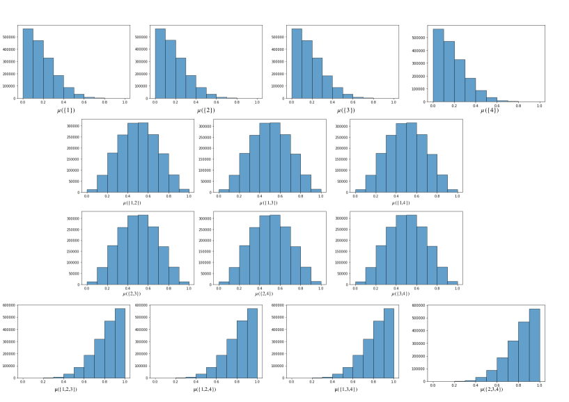
Figure 3: Histograms of $\boldsymbol{\mu}(S)$ for $n=4$ and the exact method

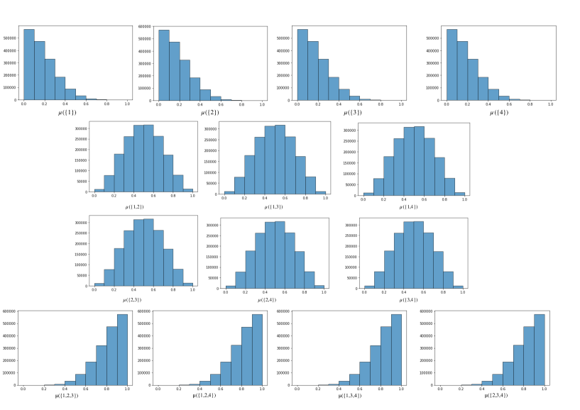
Figure 4: Histograms of $\boldsymbol{\mu}(S)$ for $n=4$ and the 2-layer approximation method

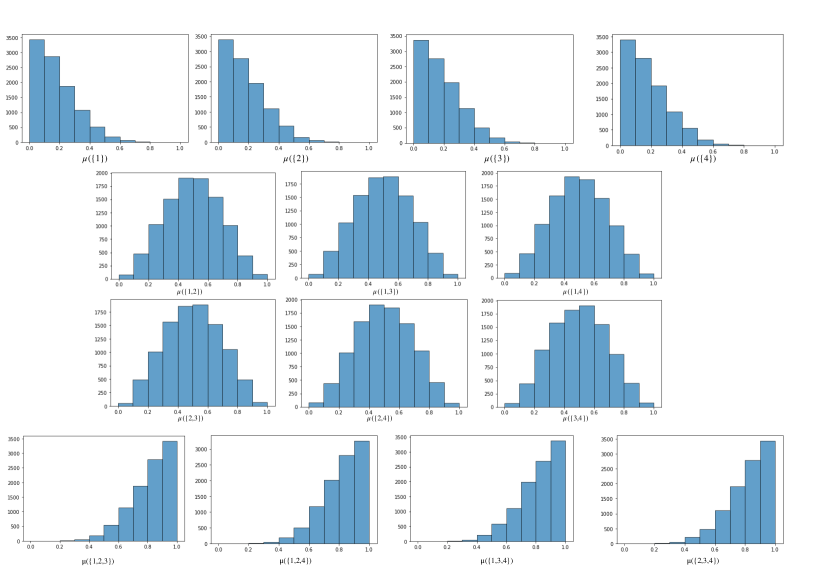
Figure 5: Histograms of $\boldsymbol{\mu}(S)$ for $n=4$ and the Markov chain method

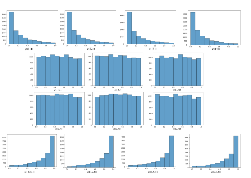
Figure 6: Histograms of $\boldsymbol{\mu}(S)$ for $n=4$ and the Random Node Generator

For comparing the histograms produced by the different methods with those of the exact methods, we use the Kullback-Leibler divergence. Given two discrete probability distribution $p,q$ on the same universe $X$, the Kullback-Leibler diveregence is defined as

$$\mathbb{D}_{KL}(p||q)=\sum_{x\in X}p(x)\log\frac{p(x)}{q(x)}.$$

The smaller the value, the closer are the two distributions. We have computed $\mathbb{D}_{KL}(p||q)$, replacing $p$ with the exact distribution and $q$ with the distribution obtained by the Markov chain method and the 2-layer approximation, respectively. Table 2 show the results for $n=4$.

capacity generator	$\mu(\{1\})$	$\mu(\{2\})$	$\mu(\{3\})$	$\mu(\{4\})$
Markov chain	0.6658	0.6698	0.6597	0.6650
2-layer approximation	0.6633	0.6614	0.6637	0.6635

capacity generator	$\mu(\{1,2\})$	$\mu(\{1,3\})$	$\mu(\{1,4\})$	$\mu(\{2,3\})$	$\mu(\{2,4\})$	$\mu(\{3,4\})$
Markov chain	0.1595	0.1593	0.1595	0.1593	0.1596	0.1593
2-layer approximation	0.1585	0.1586	0.1587	0.1586	0.1587	0.1586

capacity generator	$\mu(\{1,2,3\})$	$\mu(\{1,2,4\})$	$\mu(\{1,3,4\})$	$\mu(\{2,3,4\})$
Markov chain	0.0303	0.0304	0.0303	0.0303
2-layer approximation	0.0299	0.0300	0.0299	0.0299

Table 2: Kullback-Leibler divergence for the 2-layer approximation method and the Markov chain method compared to the exact distribution ($n=4$)

As it can be seen, the divergences obtained for the two methods are very close, with a slight advantage for the 2-layer approximation method since its values are systematically smaller.

When $n\geqslant 5$, no comparison with the exact method can be done any more, and one can only check that the properties of Lemma 2 are satisfied. Figures 7 and 8 show that histograms obtained when $n=5$ for the 2-layer approximation method and the Markov chain method. One can see that both method perform well, with a slight advantage for the 2-layer approximation method.

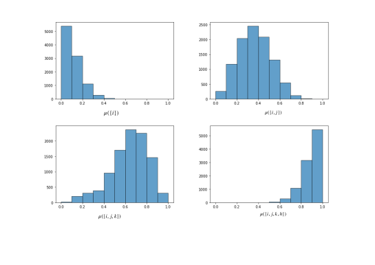
Figure 7: Histograms of $\boldsymbol{\mu}(S)$ for $n=5$ and the 2-layer approximation method

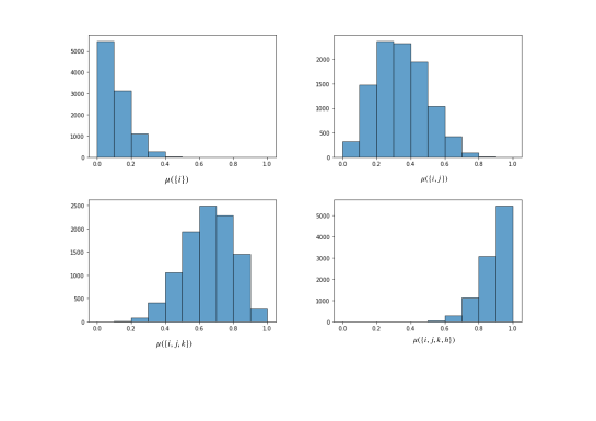
Figure 8: Histograms of $\boldsymbol{\mu}(S)$ for $n=5$ and the Markov chain method

In summary, the 2-layer approximation method and the Markov chain methods haven similar performance, with a slight advantage for the former. Concerning the computation time, however, there is a clear advantage for the 2-layer approximation method (see Table 3). Computations are done on a 3.2 GHz PC with 16 GB of RAM.

method	$n=4$	$n=5$
Two-layer approximation method	2s	13s
Markov Chain method	26s	265s

Table 3: Comparison of CPU time for generating 10000 capacities

5.2 The centroid

In order to check if the set of generated capacities is well balanced in the whole polyhedron $\mathcal{C}(N)$, we propose to compute its average capacity and to check if it coincides with the centroid of $\mathcal{C}(N)$. We recall that for a convex polyhedron $P$, the centroid can be obtained from a triangulation of the polyhedron into simplices. The centroid of a simplex is the barycenter of its vertices, and the centroid of $P$ is the average of the centroids of all simplices. Note that it differs from the barycenter of the vertices of $P$ in general.

From Section 3.1, we know that $\mathcal{C}(N)$ can be triangulated by the regions $R_{\sigma}$, each region corresponding to a linear extension, and its vertices are given by Eq. (2).

We illustrate the method of computation with $n=3$. Then, $\mathcal{C}(N)$ is a 6-dimensional polytope, triangulated into 48 simplices corresponding to the 48 linear extensions (see Table 1):

$$\sigma_{1} =\{1\},\{2\},\{3\},\{1,2\},\{1,3\},\{2,3\}$$

$$\sigma_{2} =\{1\},\{2\},\{3\},\{1,2\},\{2,3\},\{1,3\}$$

$$\sigma_{3} =\{1\},\{2\},\{3\},\{1,3\},\{1,2\},\{2,3\}$$

$$\sigma_{4} =\{1\},\{2\},\{3\},\{1,3\},\{2,3\},\{1,2\}$$

$$\sigma_{5} =\{1\},\{2\},\{3\},\{2,3\},\{1,2\},\{1,3\}$$

$$\vdots \quad\vdots$$

According to (2), the vertices of $R_{\sigma_{1}}$ are:

$$(0,0,0,0,0,0),\ (0,0,0,0,0,1),\ (0,0,0,0,1,1),\ (0,0,0,1,1,1),\ (0,0,1,1,1,1),\ (0,1,1,1,1,1),\ (1,1,1,1,1,1)$$

where the coordinates of a capacity $\mu$ in $\mathcal{C}(N)$ are given in the following order: $(\mu(\{1\})$,$\mu(\{2\})$,$\mu(\{3\})$,$\mu(\{1,2\})$, $\mu(\{1,3\})$,$\mu(\{2,3\}))$. Hence, the centroid $c_{1}$ of this simplex is the barycenter of the 7 above vertices, which yields

$$c_{1}=\Big{(}\frac{1}{7},\frac{2}{7},\frac{3}{7},\frac{4}{7},\frac{5}{7},\frac{6}{7}\Big{)}.$$

Similarly, we obtain for $R_{\sigma_{2}}$ the centroid $c_{2}$:

$$c_{2}=\Big{(}\frac{1}{7},\frac{2}{7},\frac{3}{7},\frac{4}{7},\frac{6}{7},\frac{5}{7}\Big{)}.$$

After computing the centroids of $R_{\sigma_{1}},\ldots,R_{\sigma_{48}}$, the centroid $c$ of $\mathcal{C}(N)$ is the average of all these centroids:

$$c=(0.298,0.298,0.298,0.702,0.702,0.702).$$

Exact computation can be done also for $n=4$, but not for greater values, as the number of linear extensions is too huge. Note that the centroid, whose computation is based on linear extensions, inherits the same properties as the random variables $\boldsymbol{\mu}(S)$, i.e., denoting by $c(S)$ the coordinate of $c$ pertaining to subset $S$, $c(S)$ depends only on the cardinality of $S$, and $c(N\setminus S)=1-c(S)$. This was already remarked by Miranda and Combarro [11].

Table 4 gives experimental results for $n=3$ obtained with 10000 capacities generated by the 2-layer approximation method and the Markov chain method, then averaging all of them as an estimation of the centroid. The squared error indicates the total squared error between the exact method and the considered method.

Method	centroid	squared error
exact method	(0.298, 0.298, 0.298, 0.702, 0.702, 0.702)	$-$
2-layer approximation	(0.298, 0.298, 0.296, 0.703, 0.703, 0.702)	$6\times 10^{-6}$
Markov chain	(0.297, 0.297, 0.297, 0.702, 0.703, 0.701)	$5\times 10^{-6}$

Table 4: The centroid and its estimated values for $n=3$

Table 5 is for $n=4$, and we have generated 10 times 10000 capacities in order to compute the standard deviation for the 2-layer approximation method and the Markov chain method over the 10 realizations.

Method	centroid	squared error
exact method	(0.1810, 0.1810, 0.1810, 0.1810, 0.5000, 0.5000, 0.5000, 0.5000, 0.5000, 0.5000, 0.8190, 0.8190, 0.8190, 0.8190)	$-$
2-layer approximation (mean value)	(0.1821, 0.1823, 0.1822, 0.1825, 0.5010, 0.5008, 0.5015, 0.5015, 0.5014, 0.5015, 0.8196, 0.8201 0.8204, 0.8200)	$2147\times 10^{-8}$
standard deviation	(0.0015, 0.0013, 0.0010, 0.0013, 0.0017, 0.0014, 0.0018, 0.0011, 0.0017, 0.0009, 0.0015, 0.0012, 0.0011, 0.0008)
Markov chain (mean value)	(0.1812, 0.1804, 0.1808, 0.1813, 0.5002, 0.5008, 0.5003, 0.5005, 0.5004, 0.5006, 0.8199, 0.8200, 0.8201, 0.8204)	$705\times 10^{-8}$
standard deviation	(0.0008, 0.0008, 0.0012, 0.0005, 0.0015, 0.0010, 0.0017, 0.0013, 0.0016, 0.0011, 0.0010, 0.0014, 0.0009, 0.0009)

Table 5: The centroid and its estimated values for $n=4$

Both methods show very good performance, with a slight advantage for the Markov chain method in terms of squared error when $n=4$.

5.3 Related literature

Several methods are used in the literature to measure the performance of a generator. Combarro et al. [6] use the centroid and its properties of symmetry mentioned above. They compute via an index they define if the coordinates of the average of the generated capacities are indeed depending only on the cardinality and if the symmetry $S$ vs. $N\setminus S$ is verified. This, however, is not sufficient to ensure that the averaga capacity is close to the centroid.

In [7], Combarro et al. propose to measure the total variation distance to the uniform distribution, that is to compute $\frac{1}{2}\sum_{l}|p_{l}-\frac{1}{e(p)}|$ with $p_{l}$ the probability of obtaining linear extension $l$ with a given capacity generator, and $e(p)$ is the total number of linear extensions.

Another method used in [9] is to draw the histogram and calculate the entropy of the weight $w_{\sigma(i)}$ on each source $x_{\sigma(i)}$ with $w_{\sigma(i)}=\mu(A_{i})-\mu(A_{i-1})$ and $A_{i}=\{x_{\sigma(1)},\ldots,x_{\sigma(i)}\}$. However, for the distribution of $w_{\sigma(i)}$, we only know that it holds symmetry, but nothing more is known about its properties.

Appendix A Study of posets $T_{H}$ closed under intersection

We give here a characterization of posets $T_{H}$ closed under intersection, as well as the proof of Proposition 1.

We characterize now the form of any $T_{H}$ closed under intersection. To this end, we need to distinguish two cases:

1. Situation 1: for any node $y$ of the lower layer, $|\mathsf{prec}(y)|\leq 2$.

2. Situation 2: there exists a unique $y$ of the lower layer s.t. $|\mathsf{prec}(y)|=h$, with $h$ the number of nodes in the upper layer, and $h\geqslant 3$.

We claim that under the assumption of closure under intersection, there is no other alternative.

Lemma 3.

For any $T_{H}$ closed under intersection there is no other possibility than Situations 1 and 2.

Proof.

Let $h$ be the number of nodes in the upper layer. We begin by remarking that if a node of the lower layer has $h$ predecessors, it must be unique as it is the intersection of all nodes of the upper layer.

The cases where $h=1,2$ are trivial. For $h=3$, either the number of predecessors of a lower node is at most 2, or it is 3, so either Situation 1 or 2 arises.

Assume then $h>3$. Suppose there exist a node $T$ at the lower level with $\mathsf{prec}(T)$ containing at least three nodes, say $T\cup\{1\},T\cup\{2\},T\cup\{3\}$ (therefore $T\subseteq N\setminus\{1,2,3\}$). Assume by contradiction that there exist $S$ in the upper level such that $T\not\in\mathsf{succ}(S)$. Since $T_{H}$ is closed under intersection, there must exist a successor common to $T\cup\{1\}$ and $S$. As $T\not\subseteq S$, this successor has the form $(T\setminus\{i\})\cup\{1\}$ for some $i\in T$. Therefore, $S\supseteq(T\setminus\{i\})\cup\{1\}$. Similarly, $T\cup\{2\}$ and $S$ must have a common successor, which implies that $2\in S$. Similarly, we have also that $3\in S$. Then

$$|S|\geq 3+|T\setminus\{i\}|=|T|+2,$$

which is impossible by definition of $T_{H}$. ∎

Proposition 5.

Assume $T_{H}$ is closed under intersection, let $N^{\prime}:=\bigcup_{x\in\text{upper layer}}x$, with $|N^{\prime}|=n^{\prime}\leqslant n$, and denote by $h$ the number of nodes in the upper layer, of cardinality $\ell$.

The two situations are characterized as follows:

• Situation 1:

  • Case 1: $h=1$, i.e., there is only one element in the upper layer;

  • Case 2: $h\geqslant 2$. Then $\ell=n^{\prime}-1$, i.e., the nodes of the upper layer are of the form $N^{\prime}\setminus\{i\}$. We have $\frac{h(h-1)}{2}$ nodes in the lower layer having exactly $2$ predecessors.

• Situation 2: $h=n^{\prime}-\ell+1$ and $\ell<n^{\prime}-1$. Nodes of the upper level are of the form $S\cup\{i\}$, and the lower layer contains the node $S$ with $h$ predecessors, and possibly other nodes with $0$ or $1$ predecessor.

Proof.

For Situation 1: Suppose we have $h$ nodes in the upper layer, $h\geqslant 2$. As $T_{H}$ is closed under intersection, any two nodes in the upper layer have a common successor in the lower layer. Now, in Situation 1, any node in the lower layer has at most $2$ predecessors. Hence the $\frac{h(h-1)}{2}$ pairs of nodes $x,x^{\prime}$ in the upper layer yield $\frac{h(h-1)}{2}$ distinct elements in the lower layer. Indeed, if they were not distinct, some node in the lower level would have at least $3$ predecessors.

It remains to prove that $\ell=n^{\prime}-1$. To this aim, let us take two nodes in the upper layer with common successor the set $S\subseteq N^{\prime}$. Then these two nodes must be of the form $S\cup\{i\}$ and $S\cup\{j\}$. If $h=2$, we have $N^{\prime}=S\cup\{i,j\}$, which proves the assertion. Suppose now that $h\geqslant 3$ and consider in the upper layer a set $T\neq S\cup\{i\},S\cup\{j\}$. We claim that $N^{\prime}=S\cup\{i,j\}$, i.e., $T\subseteq S\cup\{i,j\}$, which proves our assertion. Suppose by contradiction that $T$ contains an element $l$ such that $l\not\in S\cup\{i,j\}$. Let us write $T=S^{\prime}\cup\{l\}$ with $S^{\prime}\not\ni l$. As $T_{H}$ is closed under intersection, $T$ and $S\cup\{i\}$ have a common successor, which must be $S^{\prime}$, because $l$ does not belong to the successor and the successor must have $\ell-1$ elements. Similarly, the common successor of $T$ and $S\cup\{j\}$ must be $S^{\prime}$. But then $S^{\prime}$ has three predecessors, a contradiction.

For Situation 2: Denoting by $S_{1},\ldots,S_{h}$ the nodes in the upper layer, we know by definition of Situation 2 that there exists $S$ in the lower layer s.t. $S=S_{1}\cap\cdots\cap S_{h}$. Hence, the nodes in the upper layer have the form $S\cup\{i\}$ with $i\in N^{\prime}\setminus S$. Consequently, $h=n^{\prime}-|S|=n^{\prime}-\ell+1$, i.e., $\ell=n^{\prime}-h+1<n^{\prime}-1$ since $h\geqslant 3$.

Moreover, any two nodes $S\cup\{i\}$ and $S\cup\{j\}$ of the upper layer have a unique common successor, which is $S$. Hence, any $T\not=S$ in the lower layer must have $0$ or $1$ predecessor. ∎

Of course, symmetric results can be established for the two bottom layers $B_{H}$.

Figures 9 and 10 illustrate Situations 1 and 2, as well as the function $n_{x}$.

Figure 9: Situation 1.

Figure 10: Situation 2.

Proof of Proposition 1.

1. Observe that $n_{x}(0)=k-\mathsf{succ}(x)$, where $k$ is the number of nodes in the lower layer. As $n_{x}$ is invariant, $\mathsf{succ}(x)$ does not depend on $x$.

2. We distinguish two cases: Situation 1 and Situation 2.

   1. Suppose we are in Situation 1, i.e., $|\mathsf{prec}(y)|=0$, 1 or 2 for every $y$ in the lower layer. We have by definition $n_{x}(0)=k-|\mathsf{succ}(x)|$. As $|\mathsf{succ}(x)|$ is constant with $x$ by blancedness, $n_{x}(0)$ does not depend on $x$. Now, as $T_{H}[h,k,0]$ is closed under intersection, a given node $x$ has $h-1$ distinct successors $y$ given by $\mathsf{succ}(x)\cap\mathsf{succ}(x^{\prime})$ for each $x^{\prime}\neq x$ in the upper layer. Therefore $|\mathsf{prec}(y)|=2$ for each of them, so that $n_{x}(2)=h-1$. Finally, $n_{x}(1)=k-n_{x}(2)-n_{x}(0)$, which establishes the result.

   2. Suppose we are in Situation 2. From Proposition 5, we know that $|\mathsf{prec}(y)|=0$, 1 or $h$. It suffices to prove that $n_{x}$ is invariant w.r.t. $x$. We know from Proposition 5 again that there is a unique node $y$ with $|\mathsf{prec}(y)|=h$, so that clearly $n_{x}(h)=1$ for every $x$. Similarly as above, $n_{x}(0)=k-|\mathsf{succ}(x)|$, which is invariant w.r.t. $x$. Finally, $n_{x}(1)=k-n_{x}(h)-n_{x}(0)$, which establishes the result.

3. Take $T_{H}=\{123,124,23,24\}$. Then $n_{x}$ is invariant but $T_{H}$ is not closed under intersection.

4. Take $H=2^{N}\setminus\{N,\varnothing\}$, with $|N|=n$. Then $f_{x}(y)=2$ for every $y$ successor of $x$, so that clearly $n_{x}$ is invariant.

References

- [1] G. Beliakov. On random generation of supermodular capacities. IEEE Tr. on Fuzzy Systems, 30:293–296, 2022.
- [2] G. Brightwell and P. Tetali. The number of linear extensions of the Boolean lattice. Order, 20:333–345, 2003.
- [3] G. Brightwell and P. Winkler. Counting linear extensions. Order, 8:225–242, 1991.
- [4] R. Bubley and M. Dyer. Faster random generation of linear extensions. Discrete Mathematics, 201:81–88, 1999.
- [5] G. Choquet. Theory of capacities. Annales de l’Institut Fourier, 5:131–295, 1953.
- [6] E. F. Combarro, I. Díaz, and P. Miranda. On random generation of fuzzy measures. Fuzzy Sets and Systems, 228:64–77, 2013.
- [7] E. F. Combarro, J. Hurtado de Saracho, and I. Díaz. Minimals Plus: an improved algorithm for the random generation of linear extensions of partially ordered sets. Information Sciences, 501:50–67, 2019.
- [8] M. Grabisch. Set Functions, Games and Capacities in Decision Making, volume 46 of Theory and Decision Library C. Springer, 2016.
- [9] T. C. Havens and A. J. Pinar. Generating random fuzzy (capacity) measures for datafusion simulations. In IEEE Symposium Series on Computational Intelligence (IEEE SSCI2017), pages 1–8, 2017.
- [10] A. Karzanov and L. Khachiyan. On the conductance of order Markov chains. Order, 8:7–15, 1991.
- [11] P. Miranda and E. Combarro. On the structure of some families of fuzzy measures. IEEE Tr. on Fuzzy Systems, 15(6):1068–1081, 2007.
- [12] P. Miranda and P. García-Segador. Bottom-up: a new algorithm to generate random linear extensions of a poset. Order, 36:437–462, 2019.
- [13] P. Miranda and P. García-Segador. Applying Young diagrams to 2-symmetric fuzzy measures with an application to general fuzzy measures. Fuzzy Sets and Systems, 379:20–36, 2020.
- [14] P. Miranda and P. García-Segador. Combinatorial structure of the polytope of 2-additive measures. IEEE Transactions on Fuzzy Systems, 28:2864–2874, 2020.
- [15] R. Stanley. Two poset polytopes. Discrete and Computational Geometry, 1:9–23, 1986.
- [16] M. Sugeno. Theory of fuzzy integrals and its applications. PhD thesis, Tokyo Institute of Technology, 1974.
- [17] T. Talvitie, T. Niinimäki, and M. Koivisto. The mixing of Markov chains on linear extensions in practice. In Proceedings of the Twenty-Sixth International Joint Conference on Artificial Intelligence (IJCAI-17), pages 524–530, Melbourne, Australia, 2017.