1 Introduction

Monotone equations (MEs) capture a wide range of problems that include convex optimization problems, convex-concave saddle-point problems and computational models of equilibria in game-theoretic settings. Let $\mathcal{H}$ be a real Hilbert space and we define $F(x):\mathcal{H}\mapsto\mathcal{H}$ as a continuous operator. In the context of ME problem, we assume that $F$ is monotone, i.e., $\langle F(x)-F(y),x-y\rangle\geq 0$ for any $x,y\in\mathcal{H}$, and want to find a point $x^{\star}\in\mathcal{H}$ such that

$$F(x^{\star})=0.$$ (1.1)

Note that the ME problem can be equivalently formulated as unconstrained variational inequality (VI) problems corresponding to $F$ and $\mathcal{H}$ (Facchinei and Pang, 2007). In particular, we have that $x^{\star}\in\mathcal{H}$ is the solution to Eq. (1.1) if and only if we have

$$\langle F(x^{\star}),x-x^{\star}\rangle\geq 0,\quad\textnormal{for all }x\in\mathcal{H}.$$

There are many application problems that can be directly cast into the ME framework, including problems in economics and game theory (Morgenstern and Von Neumann, 1953; Fudenberg and Levine, 1998), interval arithmetic (Moore, 1979), kinematics (Morgan and Sommese, 1987), chemical engineering (Meintjes and Morgan, 1990), neurophysiology (Verschelde et al., 1994) and other engineering problems (Morgan, 2009). For an overview of recent progress on solving nonlinear equations and many more applications, we refer to Heath (2018). This line of research has recently been brought into contact with machine learning (ML), in the guise of optimality conditions for saddle-point problems, with concrete applications including robust prediction and regression (Xu et al., 2009; Esfahani and Kuhn, 2018), adversarial learning (Goodfellow et al., 2020), online learning in games (Cesa-Bianchi and Lugosi, 2006) and distributed computing (Shamma, 2008). Emerging ML applications often involve multi-agent systems, multi-way markets, or social context, and this is driving increasing interest in equilibrium formulations that can be solved as ME problems.

The classical iterative method for solving the ME problems is so-called generalized steepest descent method (Bertsekas, 1982; Hammond and Magnanti, 1987). Although this algorithm is not globally convergent for the general case where the Jacobian of $F$ is asymmetric, Hammond and Magnanti (1987) established a local linear convergence guarantee when $F$ is uniformly monotone and twice differentiable. The global convergence was proved when $F(x)=Mx-b$ and both $M$ and $M^{2}$ are positive definite. The subsequent work of Magnanti and Perakis (1997) combined the generalized steepest descent method with averaging and proved the global convergence results under weaker assumption that $M^{2}$ is semidefinite. An alternative state-of-the-art method for solving the ME problem is the Newton method which enjoys a local superlinear convergence guarantee under certain regularity conditions (Kelley, 1995, 2003). Higher-order methods were also proposed that improve upon Newton method—they are guaranteed to achieve local superquadratic convergence under the high-order Lipschitz continuity of $F$ (Homeier, 2004; Darvishi and Barati, 2007; Cordero and Torregrosa, 2007; McDougall and Wotherspoon, 2014). As for the global convergence, while it is indeed possible to give an asymptotic guarantee using line search and hyperplane projection (Solodov and Svaiter, 1999a), the global convergence rate for these methods remains unknown.

Since the ME problems are equivalent to unconstrained variational inequality (VI) problems, the VI methods can be applied with a global convergence rate guarantee. Examples include the extragradient (EG) method (Korpelevich, 1976; Nemirovski, 2004), optimistic gradient method (Popov, 1980; Mokhtari et al., 2020), dual extrapolation method (Nesterov, 2007) and other methods (Solodov and Svaiter, 1999b; Monteiro and Svaiter, 2010, 2011). All of these methods are first order and achieve the same rate of $O(1/k)$ in terms of a restricted gap function if $F$ is Lipschitz continuous. In terms of a residue function $\|F(x)\|$, the rate of $O(1/\sqrt{k})$ has been derived for the EG method (Solodov and Svaiter, 1999b; Gorbunov et al., 2022) and optimistic gradient method (Ryu et al., 2019; Kotsalis et al., 2022). It was later improved to an optimal rate of $O(1/k)$ by an anchored EG method (Yoon and Ryu, 2021). However, these existing results were restricted to first-order methods and the ME problem with a Lipschitz continuous operator. It remains unclear how to obtain global acceleration using high-order Lipschitz continuity of $F$.

As noted by Monteiro and Svaiter (2012), a global acceleration is obtained by second-order methods if $F$ is second-order Lipschitz continuous. More specifically, the $p^{\textnormal{th}}$-order methods can be used to solve the ME problems when $F$ is $p^{\textnormal{th}}$-order Lipschitz continuous (Bullins and Lai, 2022; Jiang and Mokhtari, 2022; Adil et al., 2022; Lin and Jordan, 2022b, 2023). However, the convergence analysis depends on a heuristic Lyapunov function and the global rate is only obtained in terms of a restricted gap function which is arguably less natural than a residue function for the ME problems.

This paper is motivated by the continuous-time perspective of interpreting accelerated methods as the discretization of dynamical systems. In particular, we propose novel accelerated rescaled gradient systems for characterizing global acceleration for ME problems in Eq. (1.1). Formally, our new systems can be written as follows:

$$\begin{array}[]{lll}\dot{s}(t)=-\tfrac{F(x(t))}{\|F(x(t))\|^{1-1/p}},&v(t)=x_{0}+s(t),&x(t)-v(t)+\tfrac{F(x(t))}{\|F(x(t))\|^{1-1/p}}=0,\end{array}$$ (1.2)

where $\theta>0$ and $p\in\{1,2,\ldots\}$. The initial condition is $s(0)=0$ and $x(0)=x_{0}\in\{x\in\mathcal{H}\mid F(x)\neq 0\}$. Note that this is not a restrictive condition since $F(x)=0$ implies that $x\in\mathcal{H}$ is a solution to Eq. (1.1). Throughout the paper, unless otherwise indicated, we assume that

$F:\mathcal{H}\rightarrow\mathcal{H}$ is continuous and monotone and Eq. (1.1) has at least one solution.

Our Contributions.

We summarize the main contributions of this paper as follows:

1. We show that the accelerated rescaled gradient systems in Eq. (1.2) are equivalent to closed-loop control systems (Lin and Jordan, 2023). This result is surprising since our systems are open loop without any explicit control law involved. Based on this fact, we establish the desired properties of solution trajectories, including global existence and uniqueness (see Theorem 2.2) and asymptotic weak and strong asymptotic convergence (see Theorem 2.4). Our results also include a convergence rate estimate in terms of a residue function (see Theorem 2.6).

2. We provide a unified algorithmic frameworks obtained from discretization of the system in Eq. (1.2). When combined with two different approximate subroutines it yields the classical $p^{\textnormal{th}}$-order VI methods specialized to solve ME problems (Lin and Jordan, 2022b) and new first-order methods. This highlights the advantage of our new systems over the closed-loop control systems since the resulting methods do not require line search at each iteration. We prove that the $p^{\textnormal{th}}$-order method achieves a global rate of $O(1/k^{p/2})$ in terms of $\|F(x)\|$ if $F$ is $p^{\textnormal{th}}$-order Lipschitz continuous (see Theorem 3.3) and the first-order method achieves the same global rate if $F$ is $p^{\textnormal{th}}$-order strongly Lipschitz continuous (see Theorem 3.4). If $F$ is further strongly monotone, the restarted versions of these methods can achieve a local convergence with order $p$ when $p\geq 2$ (see Theorem 3.5). All of these results are new to the best of our knowledge.

Our discrete-time analysis is largely motivated by the continuous-time analysis and demonstrates the fundamental role that rescaled gradients play in global acceleration for solving the ME problem.

Additional Related Works.

The interplay between continuous-time dynamics and discrete-time methods has been a milestone in optimization theory. A flurry of recent work in convex optimization has focused on uncovering a general principle underlying Nesterov’s accelerated gradient method (NAG) with a focus on interpreting the acceleration phenomenon using a temporal discretization of a continuous-time dynamical system with damping term (Su et al., 2016; Wibisono et al., 2016; Attouch et al., 2016b, 2018; Diakonikolas and Orecchia, 2019; Wilson et al., 2021; Muehlebach and Jordan, 2019, 2021, 2022; Shi et al., 2022; Lin and Jordan, 2022a). Among the aforementioned works, Wilson et al. (2021) found an unified time-dependent Lyapunov function and showed that their Lyapunov analysis is equivalent to Nesterov’s estimate sequence technique in a number of cases, including quasi-monotone subgradient, accelerated gradient descent and conditional gradient.

Extending the continuous-time dynamics and Lyapunov function analysis from convex optimization to monotone variational inequality and inclusion problems has been an active research area during the last two decades (Attouch and Svaiter, 2011; Maingé, 2013; Abbas et al., 2014; Attouch et al., 2013, 2016a; Attouch and László, 2020, 2021; Lin and Jordan, 2023). In particular, Attouch et al. (2016a) has proposed a second-order method for solving monotone inclusion problems but obtained a convergence rate estimate only in an optimization setting. Lin and Jordan (2023) proposed a closed-loop damping approach that generalizes Attouch et al. (2016a) and gave high-order methods with convergence rate estimates for monotone inclusion problems. In this context, the Lyapunov function has an intuitive interpretation of being the distance between the solution trajectory and an optimal solution.

Another line of works leveraged the asymptotic pseudo-trajectory (APT) theory (Benaïm and Hirsch, 1996) to push the trajectory convergence in the continuous-time dynamics to the last-iterate convergence for stochastic discrete-time methods (Benaïm et al., 2005; Mertikopoulos and Staudigl, 2018; Zhou et al., 2017, 2020). For example, Zhou et al. (2020) examined the asymptotic convergence of stochastic mirror descent (SMD) in a class of optimization problems that are not necessarily convex and proved that SMD reaches a minimum point in a finite number of steps (a.s) in problems with sharp minima. In contrast, our work presented a unified framework to develop a class of deterministic first-order and high-order methods for monotone equation problems and derive their convergence rate in terms of residue norm.

The closest work to ours is Wilson et al. (2019), who derived novel first-order optimization methods via appeal to the discretization of rescaled gradient system and proved that their accelerated methods can achieve the same global rate as accelerated high-order methods under a strong smoothness condition. While our systems in Eq. (1.2) are built upon the idea of scaling and our strong Lipschitzness condition is inspired by their condition, Wilson et al. (2019) considered a fundamentally different clas of dynamical systems without any continuous-time analysis and the derivations of their accelerated methods do not flow from a single underlying principle but tend to involve case-specific algebra.

Organization.

The remainder of the current paper is organized as follows. In Section 2, we establish global existence and uniqueness results and analyze the convergence properties of solution trajectories. In Section 3, we propose two algorithmic frameworks via appeal to the discretization of the accelerated rescaled gradient systems in Eq. (1.2), one of which when combined with an approximate tensor subroutine recovers the existing $p^{\textnormal{th}}$-order VI methods and the other of which yields a new suite of simple first-order methods. In Section 4, we provide a global convergence rate estimate in terms of a residue function. In Section 5, we conduct experiments on synthetic data to validate the efficiency of our methods. In Section 6, we conclude the paper with a discussion on future research directions.

Notation.

We use lower-case letters such as $x$ to denote vectors, and upper-case letters such as $X$ to denote tensors. We let $\mathcal{H}$ be a real Hilbert space which is endowed with an inner product $\langle\cdot,\cdot\rangle$. For $x\in\mathcal{H}$, we let $\|x\|$ denote the norm induced by $\langle\cdot,\cdot\rangle$. If $\mathcal{H}=\mathbb{R}^{d}$ is a real Euclidean space, $\|x\|$ reduces to the $\ell_{2}$-norm of $x$. Then, for $X\in\mathbb{R}^{d_{1}\times d_{2}\times\ldots\times d_{p}}$, we define

$$X[z^{1},\cdots,z^{p}]=\sum_{1\leq i_{j}\leq d_{j},1\leq j\leq p}(X_{i_{1},\cdots,i_{p}})z_{i_{1}}^{1}\cdots z_{i_{p}}^{p},$$

and let $\|X\|_{\textnormal{op}}=\max_{\|z^{i}\|=1,1\leq j\leq p}X[z^{1},\cdots,z^{p}]$. Fixing $k\geq 1$, we say $F:\mathbb{R}^{d}\rightarrow\mathbb{R}^{d}$ is $k^{\textnormal{th}}$-order Lipschitz continuous if there exists a positive constant $L>0$ such that $\|D^{(k-1)}F(x^{\prime})-D^{(k-1)}F(x)\|\leq L\|x^{\prime}-x\|$ for all $x,x^{\prime}\in\mathbb{R}^{d}$. Here, $D^{(j)}F(x)$ stands for the $j^{\textnormal{th}}$-order derivative of $F$ at $x\in\mathbb{R}^{d}$ and $D^{(0)}F=F$; indeed, for $\{z_{1},z_{2},\ldots,z_{j}\}\subseteq\mathbb{R}^{d}$, we have

$$D^{(j-1)}F(x)[z^{1},\cdots,z^{j}]=\sum_{1\leq i_{1},\ldots,i_{j}\leq d}\left[\tfrac{\partial F_{i_{1}}}{\partial x_{i_{2}}\cdots\partial x_{i_{j}}}(x)\right]z_{i_{1}}^{1}\cdots z_{i_{j}}^{j}.$$

Lastly, the notation $a=O(b(k))$ stands for an upper bound $a\leq C\cdot b(k)$, where $C>0$ is independent of the iteration count $k\in\{1,2,\ldots\}$ and $a=\tilde{O}(b(k))$ indicates the same inequality where $C>0$ might depend on the logarithmic factors of $k$.

2 Continuous-Time Accelerated Rescaled Gradient Systems

We begin by showing that the accelerated rescaled gradient systems in Eq. (1.2) are equivalent to the closed-loop control systems proposed by Lin and Jordan (2023). Based on this fact, we use dynamical systems concepts to establish the existence and uniqueness of a global solution of Eq. (1.2) and to prove asymptotic weak and strong convergence of solution trajectories. We also propose a simple yet novel Lyapunov function which we employ to derive nonasymptotic global convergence rates in terms of a residue function.

2.1 Reformulation via closed-loop control

We rewrite the accelerated rescaled gradient system in Eq. (1.2) as follows:

$$\begin{array}[]{lll}\dot{s}(t)=-\tfrac{F(x(t))}{\|F(x(t))\|^{1-1/p}},&v(t)=x_{0}+s(t),&x(t)-v(t)+\tfrac{F(x(t))}{\|F(x(t))\|^{1-1/p}}=0.\end{array}$$

Introducing the function $\lambda(t)=\frac{1}{\|F(x(t))\|^{1-1/p}}$, we have

$$\begin{array}[]{lll}\dot{s}(t)=-\lambda(t)F(x(t)),&v(t)=x_{0}+s(t),&x(t)-v(t)+\lambda(t)F(x(t))=0.\end{array}$$ (2.1)

Since $s(t)=v(t)-x_{0}$ and $s(0)=0$, we have $v(0)=x_{0}$ and

$$\dot{v}(t)=\dot{s}(t)=-\lambda(t)F(x(t))=x(t)-v(t).$$

In addition, we have $x(t)=(I+\lambda(t)F)^{-1}v(t)$. Thus, we can rewrite Eq. (2.1) as

$$\left\{\begin{array}[]{ll}&\dot{v}(t)=(I+\lambda(t)F)^{-1}v(t)-v(t),\\ &s(t)=v(t)-x_{0},\\ &x(t)=(I+\lambda(t)F)^{-1}v(t).\end{array}\right.$$

This implies that $(x,s)$ depend on the variables $(v,\lambda)$ explicitly and can be eliminated from the system. By the definition of $\lambda(\cdot)$, we have

$$1=(\lambda(t))^{p}\|F(x(t))\|^{p-1}=\lambda(t)\|\lambda(t)F(x(t))\|^{p-1}=\lambda(t)\|\dot{v}(t)\|^{p-1}.$$

Summarizing, the accelerated rescaled gradient systems in Eq. (1.2) can be equivalently reformulated as closed-loop control systems (cf. Attouch et al., 2016a; Lin and Jordan, 2023) as follows:

$$\left\{\begin{array}[]{ll}&\dot{v}(t)=(I+\lambda(t)F)^{-1}v(t)-v(t),\\ &\lambda(t)\|\dot{v}(t)\|^{p-1}=1,\\ &v(0)=x_{0}\in\Omega=\{x\in\mathcal{H}\mid F(x)\neq 0\}.\end{array}\right.$$ (2.2)

Remark 2.1

The above relationship between the accelerated rescaled gradient systems in Eq. (1.2) and the closed-loop systems in Eq. (2.2) pave the way for proving global existence and uniqueness as well as asymptotic weak and strong convergence via appeal to the existing results for closed-loop control systems studied by Lin and Jordan (2023, Theorem 2.7, 3.1 and 3.6). Such a closed-loop formulation also provides a pathway to establishing global convergence result results that are distinct from those employed in other rescaled gradient systems associated with convex optimization methods (Cortés, 2006; Wibisono et al., 2016; Wilson et al., 2019; Romero and Benosman, 2020). For further discussion of dynamical systems approaches to optimization, we refer to Romero and Benosman (2020).

2.2 Main results

We state our main theorem on the existence and uniqueness of a global solution.

Theorem 2.2

The accelerated rescaled gradient system with a fixed value of $p\geq 1$ has a unique global solution, $(x,v,s):[0,+\infty)\mapsto\mathcal{H}\times\mathcal{H}\times\mathcal{H}$. In addition, we have that $x(\cdot)$ is continuous, $v(\cdot)$ and $s(\cdot)$ are continuously differentiable, and $\|F(x(t))\|^{1/p-1}$ is nondecreasing as a function of $t$. If $p\geq 2$, we have

$$\|F(x(t))\|\geq\|F(x_{0})\|e^{-\frac{pt}{p-1}},\quad\textnormal{for all }t\geq 0.$$

Proof. By Lin and Jordan (2023, Theorem 2.7 and Lemma 2.11), the closed-loop control system in Eq. (2.2) has a unique global solution, $(v,\lambda):[0,+\infty)\mapsto\mathcal{H}\times(0,+\infty)$. In addition, $v(\cdot)$ is continuously differentiable and $\lambda(\cdot)$ is locally Lipschitz continuous and nondecreasing. If $p\geq 2$, we have

$$\|v(t)-(I+\lambda(t)F)^{-1}v(t)\|\geq\|v(0)-(I+\lambda(0)F)^{-1}v(0)\|e^{-\frac{t}{p-1}},\quad\textnormal{for all }t\geq 0.$$ (2.3)

Recall that Eq. (1.2) can be reformulated as Eq. (2.2) with the following transformations:

$$s(t)=v(t)-x_{0},\quad x(t)=(I+\lambda(t)F)^{-1}v(t),\quad\lambda(t)=\tfrac{1}{\|F(x(t))\|^{1-1/p}}.$$

Since $v(\cdot)$ is continuously differentiable, we have $s(\cdot)$ is continuously differentiable. Since $\lambda(\cdot)$ is locally Lipschitz continuous and nondecreasing, we obtain from the definition of $\lambda(t)$ that $\|F(x(t))\|^{1/p-1}$ is nondecreasing as a function of $t$. As for the relationship between $x(\cdot)$ and $v(\cdot)$, we have

$$v(t)=x(t)+\lambda(t)F(x(t))=x(t)+\tfrac{F(x(t))}{\|F(x(t))\|^{1-1/p}},$$

which implies that $\|x(t)-v(t)\|=\|F(x(t))\|^{1/p}$ and further we have

$$F(x(t))+\|x(t)-v(t)\|^{p-1}(x(t)-v(t))=0,\quad\textnormal{for all }t\geq 0.$$ (2.4)

We claim that $x(\cdot)$ is uniquely determined by $v(\cdot)$ and that $x(\cdot)$ is continuous. Indeed, let $x_{1}(t)$ and $x_{2}(t)$ both satisfy Eq. (2.4) and let $x_{1}(t_{0})\neq x_{2}(t_{0})$ for some $t_{0}>0$. For simplicity, we assume that $x_{1}=x_{1}(t_{0})$, $x_{2}=x_{2}(t_{0})$, $v=v(t_{0})$ and $\tilde{F}(\cdot)=F(\cdot)+\|\cdot-v\|^{p-1}(\cdot-v)$. Then, we have

$$\tilde{F}(x_{1})=\tilde{F}(x_{2})=0.$$

Define $f(\cdot)=\frac{1}{p+1}\|\cdot-v\|^{p+1}$, we have $\tilde{F}(\cdot)=F(\cdot)+\nabla f(\cdot)$. Since $f$ is strictly convex and $F$ is monotone, we have that $\tilde{F}$ is strictly monotone. Putting these pieces together yields that $x_{1}=x_{2}$. By the definition of $x_{1}$ and $x_{2}$, this contradicts $x_{1}(t_{0})\neq x_{2}(t_{0})$. As such, $x(\cdot)$ is uniquely determined by $v(\cdot)$.

We next prove the continuity of $x(\cdot)$ by contradiction. Assume that there exists $t_{0}>0$ such that $x(t_{n})\rightarrow\tilde{x}\neq x(t_{0})$ for some sequence $t_{n}\rightarrow t_{0}$. Note that Eq. (2.4) implies that

$$F(x(t_{n}))+\|x(t_{n})-v(t_{n})\|^{p-1}(x(t_{n})-v(t_{n}))=0.$$

Taking the limit of this equation with respect to the sequence $t_{n}$ and using the continuity of $F$ and $v(\cdot)$, we have

$$F(\tilde{x})+\|\tilde{x}-v(t_{0})\|^{p-1}(\tilde{x}-v(t_{0}))=0.$$

In addition, we have

$$F(x(t_{0}))+\|x(t_{0})-v(t_{0})\|^{p-1}(x(t_{0})-v(t_{0}))=0.$$

Combining these two equations with the previous argument implies that $\tilde{x}=x(t_{0})$ which is a contradiction. Thus, $x(\cdot)$ is continuous.

Finally, we have

$$v(t)-(I+\lambda(t)F)^{-1}v(t)=\lambda(t)F(x(t))=\tfrac{F(x(t))}{\|F(x(t))\|^{1-1/p}}.$$ (2.5)

Combining Eq. (2.3) and Eq. (2.5) implies that

$$\|F(x(t))\|^{1/p}\geq\|F(x_{0})\|^{1/p}e^{-\frac{t}{p-1}},\quad\textnormal{for all }t\geq 0.$$

which is equivalent to

$$\|F(x(t))\|\geq\|F(x_{0})\|e^{-\frac{pt}{p-1}},\quad\textnormal{for all }t\geq 0.$$

This completes the proof. $\Box$

Remark 2.3

Theorem 2.2 shows that $F(x(t))\neq 0$ for all $t\geq 0$ which is equivalent to the assertion that the orbit $x(\cdot)$ stays in $\Omega=\{x\in\mathcal{H}\mid F(x)\neq 0\}$. In other words, if $x(0)=x_{0}\in\Omega$ and $s(0)=0$ hold, the accelerated rescaled gradient systems in Eq. (1.2) can not be stabilized in finite time, which implies the asymptotic convergence behavior of corresponding discrete-time methods to an optimal solution (see Sections 3 and 4 for details). In contrast, other existing rescaled gradient systems associated with convex optimization methods (Cortés, 2006; Romero and Benosman, 2020) can exhibit finite-time convergence to an optimal solution when the function satisfies the generalized Polyak-$\L$ojasiewicz (PL) inequality.

We present our results on the asymptotic weak convergence of solution trajectories and further establish asymptotic strong convergence results under additional conditions.

Theorem 2.4

Suppose that $(x,v,s):[0,+\infty)\mapsto\mathcal{H}\times\mathcal{H}\times\mathcal{H}$ is a global solution of accelerated rescaled gradient system with a fixed value of $p\geq 1$. Then, there exists points $\bar{x}\in\{x\in\mathcal{H}\mid F(x)=0\}$ such that the solution trajectories $x(t)$ and $v(t)$ weakly converge to $\bar{x}$ as $t\rightarrow+\infty$. In addition, strong convergence results can be established if either of the following conditions holds true:

1. $F=\nabla f$ where $f:\mathcal{H}\mapsto\mathbb{R}\cup\{+\infty\}$ is convex, differentiable and inf-compact.

2. $\{x\in\mathcal{H}\mid F(x)=0\}$ has a nonempty interior.

Proof. By Lin and Jordan (2023, Theorem 3.1 and 3.6), the unique global solution $(v,\lambda)$ of the closed-loop control system in Eq. (2.2) satisfies the condition that there exists $\bar{x}\in\{x\in\mathcal{H}\mid F(x)=0\}$ such that the trajectory $v(t)$ weakly converges to $\bar{x}$ and $\|\dot{v}(t)\|\rightarrow 0$ as $t\rightarrow+\infty$. Since Eq. (1.2) can be reformulated as Eq. (2.2) with the same $v(t)$, there exist points $\bar{x}\in\{x\in\mathcal{H}\mid F(x)=0\}$ such that the solution trajectory $v(t)$ weakly converges to $\bar{x}$ as $t\rightarrow+\infty$ and the strong convergence results hold under the additional conditions stated in the theorem. Further, we see from Eq. (2.2) that $\|x(t)-v(t)\|=\|\dot{v}(t)\|\rightarrow 0$. This implies that the solution trajectory $x(t)$ weakly converges to the same $\bar{x}$ as $t\rightarrow+\infty$ with strong convergence under the same additional conditions. $\Box$

Remark 2.5

In an infinite-dimensional setting, the weak convergence of $x(\cdot)$ and $v(\cdot)$ to some points $\bar{x}\in\{x\in\mathcal{H}\mid F(x)=0\}$ in Theorem 2.4 is the best possible result we can expect without any additional conditions. However, strong convergence results are more desirable since it guarantees that the distance between the solution trajectories and $\bar{x}$ converges to 0 in terms of a norm (Bauschke and Combettes, 2001). Indeed, Güler (1991) provided an example showing the importance of strong convergence where the sequence of function values converges faster if the generated iterates achieves strong convergence. In addition, the conditions imposed by Theorem 2.4 are not restrictive and are verifiable in practice.

Before stating the main theorems on the global convergence rate, we define the residue function for the ME problems. Recalling that $x_{0}\in\Omega=\{x\in\mathcal{H}\mid F(x)\neq 0\}$ is an initial point, we define the residue function directly from the ME problem as follows:

$$\textsc{res}(x)=\|F(x)\|.$$ (2.6)

In the context of ME problems, it is arguable that this residue function serves as a more suitable optimality criterion than the celebrated merit function which was introduced by Nesterov (2007), generalizing the function gap in convex optimization problems (Facchinei and Pang, 2007).

We are now ready to present our main results on the global convergence rate estimation in terms of the residue function in Eq. (2.6).

Theorem 2.6

Suppose that $(x,v,s):[0,+\infty)\mapsto\mathcal{H}\times\mathcal{H}\times\mathcal{H}$ is a global solution of the accelerated rescaled gradient system with a fixed $p\geq 1$. Then, we have

$$\textsc{res}(x(t))=O(t^{-\frac{p}{2}}).$$

Remark 2.7

Theorem 2.6 is new and extend existing results for discrete-time first-order methods; indeed, the discrete-time version of our results for the case of $p=1$ was obtained for various first-order methods (Gorbunov et al., 2022; Kotsalis et al., 2022). Although the advantage of averaging has been well recognized in the literature (Bruck Jr, 1977; Lions, 1978; Nemirovski and Yudin, 1978; Nemirovski, 1981) and the averaged iterates can gain better rate of $O(k^{-1})$ (Ouyang and Xu, 2021), the last-iterate global convergence rate results received much attention (Mertikopoulos et al., 2018; Mertikopoulos and Zhou, 2019; Lin et al., 2020, 2021; Golowich et al., 2020a, b) and the corresponding lower complexity bound of $O(k^{-p/2})$ was recently established (Gorbunov et al., 2022; Cai et al., 2022).

We define a Lyapunov function for the system in Eq. (1.2) as follows:

$$\mathcal{E}(t)=\|s(t)\|^{2}.$$ (2.7)

Note that the function in Eq. (2.7) is the squared norm of $s(t)$ which can be seen as a continuous-time version of a dual variable in the dual extrapolation methods. This function is simpler than that used for analyzing the convergence of Newton-like inertial systems (Attouch and Svaiter, 2011; Attouch et al., 2013; Abbas et al., 2014; Attouch and László, 2020, 2021) and closed-loop control systems (Attouch et al., 2016a; Lin and Jordan, 2023). We also note that our discrete-time analysis for high-order methods largely depends on the discrete-time version of the Lyapunov function in Eq. (2.7) with a small modification to handle the constraint sets (see Section 4).

Proof of Theorem 2.6:

Using the definition of $\mathcal{E}(\cdot)$ in Eq. (2.7), we have

$$\frac{d\mathcal{E}(t)}{dt}=2\langle\dot{s}(t),s(t)\rangle=-\frac{2\langle F(x(t)),v(t)-x_{0}\rangle}{\|F(x(t))\|^{1-1/p}}.$$ (2.8)

Expanding this equality with any $z\in\mathcal{H}$, we have

$$\frac{d\mathcal{E}(t)}{dt}=\frac{2(\langle F(x(t)),x_{0}-z\rangle+\langle F(x(t)),z-x(t)\rangle+\langle F(x(t)),x(t)-v(t)\rangle)}{\|F(x(t))\|^{1-1/p}}.$$

Since $\dot{s}(t)=-\tfrac{F(x(t))}{\|F(x(t))\|^{1-1/p}}$, we have

$$\frac{\langle F(x(t)),x_{0}-z\rangle}{\|F(x(t))\|^{1-1/p}}=\langle\dot{s}(t),x_{0}-z\rangle.$$

Since $F$ is monotone, we have

$$\langle F(x(t)),z-x(t)\rangle\leq\langle F(z),z-x(t)\rangle.$$

Since $x(t)-v(t)+\tfrac{F(x(t))}{\|F(x(t))\|^{1-1/p}}=0$, we have

$$\frac{\langle F(x(t)),x(t)-v(t)\rangle}{\|F(x(t))\|^{1-1/p}}=-\|F(x(t))\|^{\frac{2}{p}}.$$

Putting these pieces together in Eq. (2.8) yields that, for any $z\in\mathcal{H}$, we have

$$\frac{d\mathcal{E}(t)}{dt}\leq 2\langle\dot{s}(t),x_{0}-z\rangle-2\|F(x(t))\|^{\frac{1-p}{p}}\langle F(z),x(t)-z\rangle-2\|F(x(t))\|^{\frac{2}{p}}.$$ (2.9)

Letting $z=\bar{x}$ be a solution satisfying $F(\bar{x})=0$ and $\|x_{0}-\bar{x}\|\leq D$ in Eq. (2.9), we have

$$\frac{d\mathcal{E}(t)}{dt}\leq 2\langle\dot{s}(t),x_{0}-\bar{x}\rangle-2\|F(x(t))\|^{\frac{2}{p}}.$$

Integrating this inequality over $[0,t]$ and using $\mathcal{E}(0)=0$, we have

$$\int_{0}^{t}\|F(x(s))\|^{\frac{2}{p}}\;ds\leq\frac{1}{2}\left(\langle s(t),x_{0}-z\rangle-\|s(t)\|^{2}\right)\leq\frac{D^{2}}{8},\quad\textnormal{for all }t\geq 0.$$

We claim that $t\mapsto\|F(x(t))\|$ is nonincreasing. Indeed, for the case of $p=1$, we have

$$\dot{s}(t)=-F(x(t)),\quad v(t)=x_{0}+s(t),\quad x(t)-v(t)+F(x(t))=0.$$

In this case, we can write $x(t)=(I+F)^{-1}v(t)$. Since $v(\cdot)$ is continuously differentiable, we have $x(\cdot)$ is also continuously differentiable. Define the function $g(t)=\frac{1}{2}\|v(t)-x(t)\|^{2}$. Then, we have

$$\dot{g}(t)=\langle\dot{v}(t)-\dot{x}(t),v(t)-x(t)\rangle=-\langle\dot{v}(t)-\dot{x}(t),\dot{v}(t)\rangle=-\|\dot{v}(t)-\dot{x}(t)\|^{2}-\langle\dot{v}(t)-\dot{x}(t),\dot{x}(t)\rangle.$$

Since $\dot{v}(t)-\dot{x}(t)=F(\dot{x}(t))$ and $F$ is monotone, we have $\langle\dot{v}(t)-\dot{x}(t),\dot{x}(t)\rangle\geq 0$. This implies that $\dot{g}(t)\leq 0$ and hence $g(t)$ is nonincreasing. For the case of $p\geq 2$, Theorem 2.2 implies that $\|F(x(t))\|^{1/p-1}$ is nondecreasing. Since $1/p-1<0$, we have $t\mapsto\|F(x(t))\|$ is nonincreasing as desired. Putting these pieces together yields that

$$\textsc{res}(x(t))=\|F(x(t))\|\leq\left(\frac{D^{2}}{8t}\right)^{\frac{p}{2}}=O(t^{-\frac{p}{2}}).$$

This completes the proof.

2.3 Discussion

In continuous-time optimization, a dynamical system is designed to be computable under the oracles of a convex and differentiable function $f:\mathcal{H}\mapsto\mathbb{R}$ such that the solution trajectory $x(t)$ converges to a minimizer of $f$. A classical example is the gradient flow in the form of $\dot{x}(t)+\nabla f(x(t))=0$ which has been long studied due to its ability to yield that $x(t)$ converges to a minimizer of $f$ as $t\rightarrow+\infty$ (Hadamard, 1908; Courant, 1943; Ambrosio et al., 2005). The subsequent work of Schropp (1995) and Schropp and Singer (2000) explored links between nonlinear dynamical systems and gradient-based optimization, including nonlinear constraints.

In his seminal work, Cortés (2006) proposed two discontinuous normalized modifications of gradient flows to attain finite-time convergence. Specifically, his dynamical systems are

$$\dot{x}(t)+\frac{\nabla f(x(t))}{\|\nabla f(x(t))\|}=0,$$ (2.10)

and

$$\dot{x}(t)+\textnormal{sign}(\nabla f(x(t)))=0.$$ (2.11)

If $f$ is twice continuously differentiable and strongly convex in an open neighborhood $D\subseteq\mathbb{R}^{n}$ of $x^{\star}$, he proved that the maximal solutions to the dynamical systems in Eq. (2.10) and (2.11) (in the sense of Filippov (Filippov, 1964; Paden and Sastry, 1987; Arscott and Filippov, 1988)) exist and converge in finite time to $x^{\star}$, given that $x_{0}$ is in some positively invariant compact subset $S\subseteq D$. The convergence times are upper bounded by

$$t^{\star}\leq\left\{\begin{array}[]{lr}\tfrac{\|\nabla f(x_{0})\|}{\min_{x\in S}\lambda_{\min}[\nabla^{2}f(x)]},&\textnormal{ for Eq.~{}\eqref{sys:NGF-first}},\\ \tfrac{\|\nabla f(x_{0})\|_{1}}{\min_{x\in S}\lambda_{\min}[\nabla^{2}f(x)]},&\textnormal{ for Eq.~{}\eqref{sys:NGF-second}}.\end{array}\right.$$

Recently, Romero and Benosman (2020) have extended the finite-time convergence results to the rescaled gradient flow proposed by Wibisono et al. (2016) as follows:

$$\dot{x}(t)+\frac{\nabla f(x(t))}{\|\nabla f(x(t))\|^{1-1/p}}=0,$$ (2.12)

and considered a new rescaled gradient flow as follows,

$$\dot{x}(t)+\|\nabla f(x(t))\|^{1/p}\textnormal{sign}(\nabla f(x(t)))=0.$$ (2.13)

In particular, if $f$ is continuously differentiable and $\mu$-gradient-dominated of order $q\in(1,p+1)$ near a strict local minimizer $x^{\star}$, the maximal solutions to the dynamical systems in Eq. (2.12) and (2.13) (in the sense of Filippov) exist and converge in finite time to $x^{\star}$, given that $\|x_{0}-x^{\star}\|>0$ is sufficiently small. The upper bounds for convergence times are summarized in Romero and Benosman (2020, Theorem 1).

However, the above works are restricted to studying the dynamical systems associated with convex optimization methods. It has been unknown whether or not these methodologies can be extended to monotone equation problems and further lead to accelerated first-order and high-order methods with global convergence rate guarantees.

3 Discrete-Time Algorithms

We propose two algorithmic frameworks that arise via temporal discretization of the systems in Eq. (1.2). Our approach highlights the importance of the dual extrapolation step (Nesterov, 2007), interpreting it as the discretization of an integral. The first framework together with an approximate tensor subroutine recovers the existing $p^{\textnormal{th}}$-order VI methods specialized to solve ME problems while the second framework yields a new suite of simple first-order methods for solving ME problems.

3.1 Temporal discretization

We begin by studying an algorithm which is derived by temporal discretization of the accelerated rescaled gradient systems in Eq. (1.2) in a Euclidean setting. In particular, the systems can be rewritten as follows,

$$\begin{array}[]{lll}\dot{s}(t)=-\tfrac{F(x(t))}{\|F(x(t))\|^{1-1/p}},&v(t)=x_{0}+s(t),&x(t)-v(t)+\tfrac{F(x(t))}{\|F(x(t))\|^{1-1/p}}=0.\end{array}$$

By introducing $\lambda(t)=\|F(x(t))\|^{1/p-1}$, we obtain

$$\left\{\begin{array}[]{ll}&\dot{s}(t)+\lambda(t)F(x(t))=0,\\ &v(t)=x_{0}+s(t),\\ &x(t)-v(t)+\tfrac{F(x(t))}{\|F(x(t))\|^{1-1/p}}=0,\\ &(\lambda(t))^{p}\|F(x(t))\|^{p-1}=1.\\ \end{array}\right.$$

Since $\|x(t)-v(t)\|=\|F(x(t))\|^{1/p}=\|\lambda(t)F(x(t))\|$, we have

$$\left\{\begin{array}[]{ll}&\dot{s}(t)+\lambda(t)F(x(t))=0,\\ &-s(t)+v(t)-x_{0}=0,\\ &F(x(t))+\|x(t)-v(t)\|^{p-1}(x(t)-v(t))=0,\\ &\lambda(t)\|x(t)-v(t)\|^{p-1}=1.\end{array}\right.$$ (3.1)

We define a sequence $\{(x_{k},v_{k+1},s_{k},\lambda_{k+1})\}_{k\geq 0}$ as a discrete-time counterpart of the solution trajectory $\{(x(t),v(t),s(t),\lambda(t))\}_{t\geq 0}$. By appeal to a discretization of the systems in Eq. (3.1), we have

$$\left\{\begin{array}[]{ll}&s_{k+1}-s_{k}+\lambda_{k+1}F(x_{k+1})=0,\\ &-s_{k}+v_{k+1}-x_{0}=0,\\ &F(x_{k+1})+\|x_{k+1}-v_{k+1}\|^{p-1}(x_{k+1}-v_{k+1})=0,\\ &\lambda_{k+1}\|x_{k+1}-v_{k+1}\|^{p-1}=1,\\ &x_{0}\in\{x\in\mathbb{R}^{d}\mid F(x)\neq 0\}\textnormal{ and }s_{0}=0.\end{array}\right.$$ (3.2)

According to the argument from Lin and Jordan (2022a), we relax the equation $\lambda_{k+1}\|x_{k+1}-v_{k+1}\|^{p-1}=1$ using $\lambda_{k+1}\|x_{k+1}-v_{k+1}\|^{p-1}\geq\theta$, where $\theta>0$ is a parameter that enhances the flexibility of our methods. It is worth mentioning that the aforementioned frameworks are intrinsically different from the large-step A-HPE framework of Monteiro and Svaiter (2012) and its high-order extension (Lin and Jordan, 2023) in that computing $x_{k+1}$ in our new frameworks do not require the value of $\lambda_{k+1}$. Indeed, the large-step A-HPE framework and its variants need to compute a pair of $x_{k+1}\in\mathbb{R}^{d}$ and $\lambda_{k+1}>0$ jointly since the computation of $x_{k+1}$ is based on $\lambda_{k+1}$ and the computation of $\lambda_{k+1}$ is based on $x_{k+1}$. This is the reason why the binary search is necessary in those frameworks.

3.2 Algorithmic schemes

By instantiating our new framework with an approximate tensor subroutine, we can recover the existing $p^{\textnormal{th}}$-order VI methods when specialized to solve ME problems (Lin and Jordan, 2022b). Indeed, the idea behind our approach is that we consider the setting where $F$ is $p^{\textnormal{th}}$-order Lipschitz continuous and define the approximate tensor subroutine based on the Taylor expansion of $F$.

Input: $p\geq 1$, $x_{0}\in\mathbb{R}^{d}$, $L>0$ and $T\geq 1$.   Initialization: $s_{0}=0\in\mathbb{R}^{d}$.   for $k=0,1,2,\ldots,T$ do      If $x_{k}$ is a solution of Eq. (1.1), then Stop.      $v_{k+1}\leftarrow x_{0}+s_{k}$.      Find $x_{k+1}$ satisfying $F_{v_{k+1}}(x_{k+1})=0$.      $\lambda_{k+1}\leftarrow\frac{\eta_{1}(p,L)}{\|x_{k+1}-v_{k+1}\|^{p-1}}$ where $\eta_{1}$ is a function.      $s_{k+1}\leftarrow s_{k}-\lambda_{k+1}F(x_{k+1})$.   end for   Output: $\bar{x}=\mathop{\rm argmin}_{x\in\{x_{0},\ldots,x_{T}\}}\|F(x)\|$. Algorithm 1 High-Order ME Methods

Input: $p\geq 1$, $x_{0}\in\mathbb{R}^{d}$, $L>0$ and $T\geq 1$.   Initialization: $s_{0}=0\in\mathbb{R}^{d}$.   for $k=0,1,2,\ldots,T$ do      If $x_{k}$ is a solution of Eq. (1.1), then Stop.      $v_{k+1}\leftarrow x_{0}+s_{k}$.      $x_{k+1}\leftarrow v_{k+1}-\gamma\|F(v_{k+1})\|^{1/p-1}F(v_{k+1})$.      $\lambda_{k+1}\leftarrow\frac{\eta_{2}(p,L,\gamma)}{\|x_{k+1}-v_{k+1}\|^{p-1}}$ where $\eta_{2}$ is a function.      $s_{k+1}\leftarrow s_{k}-\lambda_{k+1}F(x_{k+1})$.   end for   Output: $\bar{x}=\mathop{\rm argmin}_{x\in\{x_{0},\ldots,x_{T}\}}\|F(x)\|$. Algorithm 2 First-Order ME Methods

We can see from our framework that the following step plays a pivotal role:

$$\textnormal{Find }x_{k+1}\in\mathbb{R}^{d}\textnormal{ such that }F(x_{k+1})+\|x_{k+1}-v_{k+1}\|^{p-1}(x_{k+1}-v_{k+1})=0,$$

which amounts to solving a strictly monotone equation problem and which could be challenging from a computational point of view. If $F$ is $p^{\textnormal{th}}$-order Lipschitz continuous, we can approximate $F(x_{k+1})$ using the Taylor expansion of $F$ at a point $v\in\mathbb{R}^{d}$. That is, we define

$$F_{v}(x)=F(v)+\langle DF(v),x-v\rangle+\ldots+\tfrac{1}{(p-1)!}D^{(p-1)}F(v)[x-v]^{p-1}+\tfrac{2L}{(p-1)!}\|x-v\|^{p-1}(x-v),$$ (3.3)

and consider the following subproblem given by

$$\textnormal{Find }x_{k+1}\in\mathbb{R}^{d}\textnormal{ such that }F_{v_{k+1}}(x_{k+1})=0.$$

The resulting $p^{\textnormal{th}}$-order methods recover the existing $p^{\textnormal{th}}$-order VI methods when specialized to solve ME problems (Lin and Jordan, 2022b) and we summarize the details in Algorithm 1. For simplicity, we assume an access to an oracle which returns an exact solution of each subproblem and do not take the inexact approaches into account.

Following the idea of Wilson et al. (2019), we also approximate $F(x_{k+1})$ using the first-order Taylor expansion of $F$ at a point $v\in\mathbb{R}^{d}$ and consider another subproblem given by

$$\textnormal{Find }x_{k+1}\in\mathbb{R}^{d}\textnormal{ such that }F(v_{k+1})+\tfrac{1}{\gamma^{p}}\|x_{k+1}-v_{k+1}\|^{p-1}(x_{k+1}-v_{k+1})=0.$$

This yields a new suite of simple first-order methods where each subproblem admits a closed-form solution. We summarize the details in Algorithm 2.

We also summarize the restarted versions of two above ME methods in Algorithm 3, which is built upon the restart strategy. Suppose that $F$ is strongly monotone around a unique optimal solution and $p\geq 2$, we consider Algorithm 3 and prove that it achieves a local superlinear convergence. Concerning Algorithm 3, we run one iteration of Algorithm 1 and 2 initialized with $x_{k}$ at each epoch; indeed, we simply restart Algorithm 1 and 2 properly. It is also promising to combine our methods with adaptive restart strategies (O’donoghue and Candes, 2015; Roulet and d’Aspremont, 2017), and/or prove a local convergence guarantee under weaker conditions than the strong monotonicity of $F$.

  Input: $p\geq 1$, $x_{0}\in\mathbb{R}^{d}$, $L>0$ and $T\geq 1$.

  for $k=0,1,2,\ldots,T$ do

     If $x_{k}$ is a solution of Eq. (1.1), then Stop.

     $x_{k+1}$ is an output of Algorithms 1 and 2 with $(p,x_{k},L,1)$, i.e., one iteration but initialized with $x_{k}$.

  end for

Algorithm 3 The Restart Versions of Algorithms 1 and 2

3.3 Main results

We start with the presentation of our main results for Algorithm 1 and 2. To facilitate the presentation, we rewrite the definition of a residue function as $\textsc{res}(x)=\|F(x)\|$ and also recall the definitions of $p^{\textnormal{th}}$-order Lipschitz continuous and $p^{\textnormal{th}}$-order strongly Lipschitz continuous operators as follows.

Definition 3.1

$F$ is $p^{\textnormal{th}}$-order Lipschitz continuous if $\|D^{(p-1)}F(x^{\prime})-D^{(p-1)}F(x)\|\leq L\|x^{\prime}-x\|$.

Definition 3.2

$F$ is $p^{\textnormal{th}}$-order strongly Lipschitz continuous if $\|D^{(p-1)}F(x^{\prime})-D^{(p-1)}F(x)\|\leq L\|x^{\prime}-x\|$ and $\|D^{(m)}F(x)[F(x)]^{m}\|\leq L\|F(x)\|^{m+1-m/p}$ for $1\leq m\leq p-1$.

We summarize our results in the following theorems.

Theorem 3.3

Letting $F$ be monotone and $p^{\textnormal{th}}$-order Lipschitz continuous and we set $\frac{p!}{(12p-6)L}\leq\eta_{1}(p,L)\leq\frac{p!}{(4p+2)L}$ in Algorithm 1. Then, the iterates $\{x_{k}\}_{k\geq 0}$ generated by the algorithm satisfy

$$\inf_{0\leq i\leq k}\textsc{res}(x_{i})=O(k^{-\frac{p}{2}}).$$

Theorem 3.4

Letting $F$ be monotone and $p^{\textnormal{th}}$-order strongly Lipschitz continuous and we set $\frac{\gamma^{p}}{6-6\gamma Lc_{p}}\leq\eta_{2}(p,L,\gamma)\leq\frac{\gamma^{p}}{2+2\gamma Lc_{p}}$ where $0<\gamma<\min\{1,\frac{1}{2Lc_{p}}\}$ with $c_{p}=\sum_{m=1}^{p}\tfrac{1}{m!}$ in Algorithm 2. Then, the iterates $\{x_{k}\}_{k\geq 0}$ generated by the algorithm satisfy

$$\inf_{0\leq i\leq k}\textsc{res}(x_{i})=O(k^{-\frac{p}{2}}).$$

The local convergence guarantee for Algorithm 3 when $p\geq 2$ was established in the following theorem. Our analysis is based on Theorem 3.3 and 3.4 and our results are expressed in terms of $\|x_{k}-x^{\star}\|$, where $x^{\star}\in\mathbb{R}^{d}$ is a unique solution of Eq. (1.1) in the sense that $F(x^{\star})=0$.

Theorem 3.5

Suppose that $F$ be $\mu$-strongly monotone. Then, the following statements hold true.

• Under the same assumption as in Theorem 3.3, the iterates $\{x_{k}\}_{k\geq 0}$ generated by Algorithm 3 with Algorithm 1 as the subroutine satisfy

  $$\|x_{k+1}-x^{\star}\|\leq\left(\tfrac{4^{p}(2p+1)}{p!}\tfrac{L}{\mu}\right)\|x_{k}-x^{\star}\|^{p},\quad\textnormal{for all }k\geq 0.$$

  As a consequence, the above iterates $\{x_{k}\}_{k\geq 0}$ converge with a rate at least of the order $p\geq 2$ if the following condition holds true:

  $$\|x_{0}-x^{\star}\|\leq\tfrac{1}{2}\left(\tfrac{p!}{4^{p}(2p+1)}\tfrac{\mu}{L}\right)^{\frac{1}{p-1}}.$$

• Under the same assumption as in Theorem 3.4, the iterates $\{x_{k}\}_{k\geq 0}$ generated by Algorithm 3 with Algorithm 2 as the subroutine satisfy

  $$\|x_{k+1}-x^{\star}\|\leq\left(\tfrac{2^{2p+1}}{\mu\gamma^{p}}\right)\|x_{k}-x^{\star}\|^{p},\quad\textnormal{for all }k\geq 0.$$

  As a consequence, the above iterates $\{x_{k}\}_{k\geq 0}$ converge with a rate at least of the order $p\geq 2$ if the following condition holds true:

  $$\|x_{0}-x^{\star}\|\leq\tfrac{1}{2}\left(\tfrac{\mu\gamma^{p}}{2^{2p+1}}\right)^{\frac{1}{p-1}}.$$

Remark 3.6

Theorem 3.3 improves the convergence rate of $O(k^{-(p+1)/2}\log(k))$ which was obtained for $p^{\textnormal{th}}$-order line-search-based methods (Lin and Jordan, 2023) under the same assumptions. The local convergence guarantee in Theorem 3.5 has been derived by Jiang and Mokhtari (2022) for generalized optimistic gradient methods but without counting the required number of binary searches at each iteration.

Remark 3.7

Theorem 3.4 and 3.5 are new and can be understood as a generalization of Wilson et al. (2019) from unconstrained convex optimization problems to monotone equation problems. There are also examples of strongly Lipschitz continuous operators in machine learning and we refer to Wilson et al. (2019) for concrete examples and relevant discussion.

Remark 3.8

The anchored extragradient method from Yoon and Ryu (2021) was shown to achieve an optimal convergence rate of $O(1/k)$ in terms of $\|F(x)\|$ and thus outperforms Algorithm 1 for the case of $p=1$. Can we interpret the anchoring scheme from a continuous-time viewpoint and develop a high-order anchored method with an improved convergence rate guarantee? We leave this for future work and believe this would be a worthwhile research problem that deserves a specialized treatment on its own.

4 Discrete-Time Convergence Analysis

We conduct the discrete-time convergence analysis for Algorithm 1 and 2. In terms of a residue function, we prove a global rate of $O(k^{-p/2})$ for Algorithm 1 if $F$ is $p^{\textnormal{th}}$-order Lipschitz continuous and Algorithm 2 if $F$ is $p^{\textnormal{th}}$-order strongly Lipschitz continuous. Our analysis is motivated by the continuous-time analysis from Section 2 and thus differs from the previous analysis in Lin and Jordan (2022b).

4.1 Proof of Theorem 3.3

We construct a discrete-time Lyapunov function for Algorithm 1 as follows:

$$E_{k}=\tfrac{1}{2}\|s_{k}\|^{2},$$ (4.1)

which will be used to prove several technical lemmas for proving Theorem 3.3.

Lemma 4.1

For every integer $T\geq 1$, we have

$$\sum_{k=1}^{T}\lambda_{k}\langle F(x_{k}),x_{k}-x\rangle\leq E_{0}-E_{T}+\langle s_{T},x-x_{0}\rangle-\tfrac{1}{10}\left(\sum_{k=1}^{T}\|x_{k}-v_{k}\|^{2}\right),\quad\textnormal{for all }x\in\mathbb{R}^{d}.$$

Proof. We have

$$E_{k+1}-E_{k}=\langle s_{k+1}-s_{k},s_{k+1}\rangle-\tfrac{1}{2}\|s_{k+1}-s_{k}\|^{2}.$$

Combining this equation with the definition of $v_{k+1}$, we have

$$E_{k+1}-E_{k}=\lambda_{k+1}\langle F(x_{k+1}),x_{0}-v_{k+2}\rangle-\tfrac{1}{2}\|v_{k+2}-v_{k+1}\|^{2}.$$

Letting $x\in\mathbb{R}^{d}$, we have

$$E_{k+1}-E_{k}\leq\lambda_{k+1}\langle F(x_{k+1}),x_{0}-x\rangle+\lambda_{k+1}\langle F(x_{k+1}),x-x_{k+1}\rangle+\lambda_{k+1}\langle F(x_{k+1}),x_{k+1}-v_{k+2}\rangle-\tfrac{1}{2}\|v_{k+2}-v_{k+1}\|^{2}.$$

Summing up this inequality over $k=0,1,\ldots,T-1$ and changing the counter $k+1$ to $k$ yields

$$\sum_{k=1}^{T}\lambda_{k}\langle F(x_{k}),x_{k}-x\rangle\leq E_{0}-E_{T}+\underbrace{\sum_{k=1}^{T}\lambda_{k}\langle F(x_{k}),x_{0}-x\rangle}_{\textbf{I}}+\underbrace{\sum_{k=1}^{T}\lambda_{k}\langle F(x_{k}),x_{k}-v_{k+1}\rangle-\tfrac{1}{2}\|v_{k}-v_{k+1}\|^{2}}_{\textbf{II}}.$$ (4.2)

Using the update formula $s_{k+1}=s_{k}-\lambda_{k+1}F(x_{k+1})$ and $s_{0}=0\in\mathbb{R}^{d}$, we have

$$\textbf{I}=\langle s_{0}-s_{T},x_{0}-x\rangle=\langle s_{T},x-x_{0}\rangle.$$ (4.3)

Recall that $F_{v_{k}}(x_{k})=0$ where $F_{v}(x):\mathbb{R}^{d}\rightarrow\mathbb{R}^{d}$ is defined with any fixed $v\in\mathcal{X}$ as follows,

$$F_{v}(x)=F(v)+\langle DF(v),x-v\rangle+\ldots+\tfrac{1}{(p-1)!}D^{(p-1)}F(v)[x-v]^{p-1}+\tfrac{2L}{(p-1)!}\|x-v\|^{p-1}(x-v).$$

Since $F$ is $p^{\textnormal{th}}$-order Lipschitz continuous, we have

$$\|F(x_{k})-F_{v_{k}}(x_{k})+\tfrac{2L}{(p-1)!}\|x_{k}-v_{k}\|^{p-1}(x_{k}-v_{k})\|\leq\tfrac{L}{p!}\|x_{k}-v_{k}\|^{p}.$$ (4.4)

We perform a decomposition of $\langle F(x_{k}),x_{k}-v_{k+1}\rangle$ and derive from Eq. (4.4) that

$$\langle F(x_{k}),x_{k}-v_{k+1}\rangle$$

$$= \langle F(x_{k})-F_{v_{k}}(x_{k})+\tfrac{2L}{(p-1)!}\|x_{k}-v_{k}\|^{p-1}(x_{k}-v_{k}),x_{k}-v_{k+1}\rangle-\tfrac{2L}{(p-1)!}\|x_{k}-v_{k}\|^{p-1}\langle x_{k}-v_{k},x_{k}-v_{k+1}\rangle$$

$$\leq \|F(x_{k})-F_{v_{k}}(x_{k})+\tfrac{2L}{(p-1)!}\|x_{k}-v_{k}\|^{p-1}(x_{k}-v_{k})\|\|x_{k}-v_{k+1}\|-\tfrac{2L}{(p-1)!}\|x_{k}-v_{k}\|^{p-1}\langle x_{k}-v_{k},x_{k}-v_{k+1}\rangle$$

$$\leq \tfrac{L}{p!}\|x_{k}-v_{k}\|^{p}\|x_{k}-v_{k+1}\|-\tfrac{2L}{(p-1)!}\|x_{k}-v_{k}\|^{p-1}\langle x_{k}-v_{k},x_{k}-v_{k+1}\rangle\quad\textnormal{(cf. Eq.~{}\eqref{inequality:HO-descent-third})}$$

$$\leq \tfrac{L}{p!}\|x_{k}-v_{k}\|^{p+1}+\tfrac{L}{p!}\|x_{k}-v_{k}\|^{p}\|v_{k}-v_{k+1}\|-\tfrac{2L}{(p-1)!}\|x_{k}-v_{k}\|^{p-1}\langle x_{k}-v_{k},x_{k}-v_{k+1}\rangle.$$

Note that we have

$$\langle x_{k}-v_{k},x_{k}-v_{k+1}\rangle=\|x_{k}-v_{k}\|^{2}+\langle x_{k}-v_{k},v_{k}-v_{k+1}\rangle\geq\|x_{k}-v_{k}\|^{2}-\|x_{k}-v_{k}\|\|v_{k}-v_{k+1}\|.$$

Putting these pieces together yields that

$$\langle F(x_{k}),x_{k}-v_{k+1}\rangle\leq\tfrac{(2p+1)L}{p!}\|x_{k}-v_{k}\|^{p}\|v_{k}-v_{k+1}\|-\tfrac{(2p-1)L}{p!}\|x_{k}-v_{k}\|^{p+1}.$$

Since $\lambda_{k}=\frac{\eta_{1}(p,L)}{\|x_{k}-v_{k}\|^{p-1}}$ and $\frac{p!}{(12p-6)L}\leq\eta_{1}(p,L)\leq\frac{p!}{(4p+2)L}$, we have $\frac{1}{12p-6}\leq\frac{\lambda_{k}L\|x_{k}-v_{k}\|^{p-1}}{p!}\leq\frac{1}{4p+2}$. Thus, we have

II $$\leq \sum_{k=1}^{T}\left(\tfrac{(2p+1)\lambda_{k}L}{p!}\|x_{k}-v_{k}\|^{p}\|\|v_{k}-v_{k+1}\|-\tfrac{1}{2}\|v_{k}-v_{k+1}\|^{2}-\tfrac{(2p-1)\lambda_{k}L}{p!}\|x_{k}-v_{k}\|^{p+1}\right)$$ (4.5)

$$\leq \sum_{k=1}^{T}\left(\tfrac{1}{2}\|x_{k}-v_{k}\|\|\|v_{k}-v_{k+1}\|-\tfrac{1}{2}\|v_{k}-v_{k+1}\|^{2}-\tfrac{1}{6}\|x_{k}-v_{k}\|^{2}\right)$$

$$\leq \sum_{k=1}^{T}\left(\max_{a\geq 0}\left\{\tfrac{1}{2}\|x_{k}-v_{k}\|a-\tfrac{1}{2}a^{2}\right\}-\tfrac{1}{6}\|x_{k}-v_{k}\|^{2}\right)$$

$$= -\tfrac{1}{24}\left(\sum_{k=1}^{T}\|x_{k}-v_{k}\|^{2}\right).$$

Plugging Eq. (4.3) and Eq. (4.5) into Eq. (4.2) yields that

$$\sum_{k=1}^{T}\lambda_{k}\langle F(x_{k}),x_{k}-x\rangle\leq E_{0}-E_{T}+\langle s_{T},x-x_{0}\rangle-\tfrac{1}{24}\left(\sum_{k=1}^{T}\|x_{k}-v_{k}\|^{2}\right).$$

This completes the proof. $\Box$

Lemma 4.2

For every integer $T\geq 1$ and let $x\in\mathbb{R}^{d}$, we have

$$\sum_{k=1}^{T}\|x_{k}-v_{k}\|^{2}\leq 12\|x^{\star}-x_{0}\|^{2},$$

where $x^{\star}\in\mathbb{R}^{d}$ is a solution of Eq. (1.1) satisfying that $F(x^{\star})=0$.

Proof. For any $x\in\mathbb{R}^{d}$, we have

$$E_{0}-E_{T}+\langle s_{T},x-x_{0}\rangle=E_{0}-\tfrac{1}{2}\|s_{T}\|^{2}+\langle s_{T},x-x_{0}\rangle.$$

Since $s_{0}=0$, we have $E_{0}=0$. By Young’s inequality, we have

$$E_{0}-E_{T}+\langle s_{T},x-x_{0}\rangle\leq-\tfrac{1}{2}\|s_{T}\|^{2}+\tfrac{1}{2}\|s_{T}\|^{2}+\tfrac{1}{2}\|x-x_{0}\|^{2}=\tfrac{1}{2}\|x-x_{0}\|^{2}.$$

This together with Lemma 4.1 yields that

$$\sum_{k=1}^{T}\lambda_{k}\langle F(x_{k}),x_{k}-x\rangle+\tfrac{1}{24}\left(\sum_{k=1}^{T}\|x_{k}-v_{k}\|^{2}\right)\leq\tfrac{1}{2}\|x-x_{0}\|^{2},\quad\textnormal{for all }x\in\mathbb{R}^{d},$$

which implies the first inequality. Letting $x=x^{\star}$ be a solution of Eq. (1.1) satisfying that $F(x^{\star})=0$ in the above inequality yields the desired inequality. $\Box$

Proof of Theorem 3.3:

We let $x^{\star}\in\mathbb{R}^{d}$ be a solution of Eq. (1.1) defined in Lemma 4.2 and have

$$\inf_{1\leq k\leq T}\|x_{k}-v_{k}\|^{2}\leq\tfrac{1}{T}\sum_{k=1}^{T}\|x_{k}-v_{k}\|^{2}\leq\tfrac{12\|x^{\star}-x_{0}\|^{2}}{T}.$$ (4.6)

Recall that Eq. (4.4) in the proof of Lemma 4.1 yields

$$\|F(x_{k})-F_{v_{k}}(x_{k})+\tfrac{2L}{(p-1)!}\|x_{k}-v_{k}\|^{p-1}(x_{k}-v_{k})\|\leq\tfrac{L}{p!}\|x_{k}-v_{k}\|^{p}.$$

Since $F_{v_{k}}(x_{k})=0$, we have

$$\|F(x_{k})\|\leq\tfrac{L}{p!}\|x_{k}-v_{k}\|^{p}+\tfrac{2L}{(p-1)!}\|x_{k}-v_{k}\|^{p}\leq\tfrac{(2p+1)L}{p!}\|x_{k}-v_{k}\|^{p}.$$

By the definition of $\textsc{res}(\cdot)$, we have

$$\inf_{1\leq k\leq T}\textsc{res}(x_{k})=\inf_{1\leq k\leq T}\|F(x_{k})\|\leq\tfrac{(2p+1)L}{p!}\left(\inf_{1\leq k\leq T}\|x_{k}-v_{k}\|^{p}\right).$$ (4.7)

Plugging Eq. (4.6) into Eq. (4.7) yields the desired result.

4.2 Proof of Theorem 3.4

We use the same discrete-time Lyapunov function in Eq. (4.1) to analyze the dynamics of Algorithm 2.

Lemma 4.3

For every integer $T\geq 1$, we have

$$\sum_{k=1}^{T}\lambda_{k}\langle F(x_{k}),x_{k}-x\rangle\leq E_{0}-E_{T}+\langle s_{T},x-x_{0}\rangle-\tfrac{1}{10}\left(\sum_{k=1}^{T}\|x_{k}-v_{k}\|^{2}\right),\quad\textnormal{for all }x\in\mathbb{R}^{d}.$$

Proof. Using the same arguments as in Lemma 4.1, we have

$$\sum_{k=1}^{T}\lambda_{k}\langle F(x_{k}),x_{k}-x\rangle\leq E_{0}-E_{T}+\langle s_{T},x-x_{0}\rangle+\underbrace{\sum_{k=1}^{T}\lambda_{k}\langle F(x_{k}),x_{k}-v_{k+1}\rangle-\tfrac{1}{2}\|v_{k}-v_{k+1}\|^{2}}_{\textbf{III}}.$$ (4.8)

Recall that $x_{k}=v_{k}-\gamma\|F(v_{k})\|^{1/p-1}F(v_{k})$, we have

$$x_{k}-v_{k}=-\gamma\|F(v_{k})\|^{1/p-1}F(v_{k}).$$ (4.9)

We perform a decomposition of $\|F(x_{k})-F(v_{k})\|$ and derive from Eq. (4.9) that

$$\|F(x_{k})-F(v_{k})\|\leq\|F(x_{k})-F(v_{k})-\sum_{m=1}^{p-1}\tfrac{1}{m!}D^{(m)}F(v_{k})[x_{k}-v_{k}]^{m}\|+\sum_{m=1}^{p-1}\tfrac{1}{m!}|D^{(m)}F(v_{k})[x_{k}-v_{k}]^{m}|$$

$$= \|F(x_{k})-F(v_{k})-\sum_{m=1}^{p-1}\tfrac{1}{m!}D^{(m)}F(v_{k})[x_{k}-v_{k}]^{m}\|+\sum_{m=1}^{p-1}\tfrac{\gamma^{m}}{m!}\|F(v_{k})\|^{\frac{m(1-p)}{p}}|D^{(m)}F(v_{k})[F(v_{k})]^{m}|.$$

Since $F$ is $p^{\textnormal{th}}$-order strongly Lipschitz continuous, we have

$$\|F(x_{k})-F(v_{k})-\sum_{m=1}^{p-1}\tfrac{1}{m!}D^{(m)}F(v_{k})[x_{k}-v_{k}]^{m}\|\leq\tfrac{L}{p!}\|x_{k}-v_{k}\|^{p},$$

and

$$\sum_{m=1}^{p-1}\tfrac{\gamma^{m}}{m!}\|F(v_{k})\|^{\frac{m(1-p)}{p}}|D^{(m)}F(v_{k})[F(v_{k})]^{m}|\leq\left(\sum_{m=1}^{p-1}\tfrac{\gamma^{m}}{m!}\right)L\|F(v_{k})\|=\left(\sum_{m=1}^{p-1}\tfrac{\gamma^{m-p}}{m!}\right)L\|x_{k}-v_{k}\|^{p}.$$

Since $0<\gamma<1$, we have

$$\|F(x_{k})-F(v_{k})\|\leq\left(\sum_{m=1}^{p}\tfrac{\gamma^{m-p}}{m!}\right)L\|x_{k}-v_{k}\|^{p}\leq\tfrac{1}{\gamma^{p-1}}\left(\sum_{m=1}^{p}\tfrac{1}{m!}\right)L\|x_{k}-v_{k}\|^{p}.$$ (4.10)

For simplicity, we let $c_{p}=\sum_{m=1}^{p}\tfrac{1}{m!}$. By using the argument as in Lemma 4.1 with Eq. (4.9) and (4.10), we have

$$\langle F(x_{k}),x_{k}-v_{k+1}\rangle=\langle F(x_{k})-F(v_{k}),x_{k}-v_{k+1}\rangle+\langle F(v_{k}),x_{k}-v_{k+1}\rangle$$

$$\leq \langle F(x_{k})-F(v_{k}),x_{k}-v_{k+1}\rangle-\tfrac{1}{\gamma^{p}}\|x_{k}-v_{k}\|^{p-1}\langle x_{k}-v_{k},x_{k}-v_{k+1}\rangle\quad\textnormal{(cf. Eq.~{}\eqref{inequality:FO-descent-second})}$$

$$\leq \tfrac{Lc_{p}}{\gamma^{p-1}}\|x_{k}-v_{k}\|^{p}\|x_{k}-v_{k+1}\|-\tfrac{1}{\gamma^{p}}\|x_{k}-v_{k}\|^{p-1}\langle x_{k}-v_{k},x_{k}-v_{k+1}\rangle\quad\textnormal{(cf. Eq.~{}\eqref{inequality:FO-descent-third})}$$

$$\leq \tfrac{Lc_{p}}{\gamma^{p-1}}\|x_{k}-v_{k}\|^{p+1}+\tfrac{Lc_{p}}{\gamma^{p-1}}\|x_{k}-v_{k}\|^{p}\|v_{k}-v_{k+1}\|-\tfrac{1}{\gamma^{p}}\|x_{k}-v_{k}\|^{p-1}\langle x_{k}-v_{k},x_{k}-v_{k+1}\rangle.$$

Since $\langle x_{k}-v_{k},x_{k}-v_{k+1}\rangle\geq\|x_{k}-v_{k}\|^{2}-\|x_{k}-v_{k}\|\|v_{k}-v_{k+1}\|$, we have

$$\langle F(x_{k}),x_{k}-v_{k+1}\rangle\leq\tfrac{1+\gamma Lc_{p}}{\gamma^{p}}\|x_{k}-v_{k}\|^{p}\|v_{k}-v_{k+1}\|-\tfrac{1-\gamma Lc_{p}}{\gamma^{p}}\|x_{k}-v_{k}\|^{p+1}.$$

Since $0<\gamma<\frac{1}{2Lc_{p}}$, the interval $[\tfrac{\gamma^{p}}{6-6\gamma Lc_{p}},\tfrac{\gamma^{p}}{2+2\gamma Lc_{p}}]$ is nonempty. Thus, it would be reasonable to define the function $\eta_{2}(p,L,\gamma)$ satisfying that

$$\tfrac{\gamma^{p}}{6-6\gamma Lc_{p}}\leq\eta_{2}(p,L,\gamma)\leq\tfrac{\gamma^{p}}{2+2\gamma Lc_{p}}.$$

Since $\lambda_{k}=\frac{\eta_{2}(p,L,\gamma)}{\|x_{k}-v_{k}\|^{p-1}}$, we have $\frac{1}{6-6\gamma Lc_{p}}\leq\frac{\lambda_{k}\|x_{k}-v_{k}\|^{p-1}}{\gamma^{p}}\leq\frac{1}{2+2\gamma Lc_{p}}$. This yields

III $$\leq \sum_{k=1}^{T}\left(\tfrac{1+\gamma Lc_{p}}{\gamma^{p}}\lambda_{k}\|x_{k}-v_{k}\|^{p}\|v_{k}-v_{k+1}\|-\tfrac{1}{2}\|v_{k}-v_{k+1}\|^{2}-\tfrac{1-\gamma Lc_{p}}{\gamma^{p}}\lambda_{k}\|x_{k}-v_{k}\|^{p+1}\right)$$ (4.11)

$$\leq \sum_{k=1}^{T}\left(\tfrac{1}{2}\|x_{k}-v_{k}\|\|\|v_{k}-v_{k+1}\|-\tfrac{1}{2}\|v_{k}-v_{k+1}\|^{2}-\tfrac{1}{6}\|x_{k}-v_{k}\|^{2}\right)$$

$$\leq \sum_{k=1}^{T}\left(\max_{a\geq 0}\left\{\tfrac{1}{2}\|x_{k}-v_{k}\|a-\tfrac{1}{2}a^{2}\right\}-\tfrac{1}{6}\|x_{k}-v_{k}\|^{2}\right)$$

$$= -\tfrac{1}{24}\left(\sum_{k=1}^{T}\|x_{k}-v_{k}\|^{2}\right).$$

Plugging Eq. (4.11) into Eq. (4.8) yields that

$$\sum_{k=1}^{T}\lambda_{k}\langle F(x_{k}),x_{k}-x\rangle\leq E_{0}-E_{T}+\langle s_{T},x-x_{0}\rangle-\tfrac{1}{24}\left(\sum_{k=1}^{T}\|x_{k}-v_{k}\|^{2}\right).$$

This completes the proof. $\Box$

Proof of Theorem 3.4:

Since Lemma 4.3 guarantees that Lemma 4.2 still holds true for Algorithm 2, we have

$$\inf_{1\leq k\leq T}\|x_{k}-v_{k}\|^{2}\leq\tfrac{12\|x^{\star}-x_{0}\|^{2}}{T}.$$ (4.12)

Recall that Eq. (4.10) in the proof of Lemma 4.3 yields

$$\|F(x_{k})-F(v_{k})\|\leq\tfrac{1}{\gamma^{p-1}}\left(\sum_{m=1}^{p}\tfrac{1}{m!}\right)L\|x_{k}-v_{k}\|^{p}.$$

Since $0<\gamma<\frac{1}{2Lc_{p}}$ where $c_{p}=\sum_{m=1}^{p}\tfrac{1}{m!}$, we have

$$\|F(x_{k})-F(v_{k})\|\leq\tfrac{1}{2\gamma^{p}}\|x_{k}-v_{k}\|^{p}.$$

Recall that $x_{k}=v_{k}-\gamma\|F(v_{k})\|^{1/p-1}F(v_{k})$ yields $\|F(v_{k})\|=\frac{1}{\gamma^{p}}\|x_{k}-v_{k}\|^{p}$, we have

$$\|F(x_{k})\|\leq\tfrac{1}{\gamma^{p}}\|x_{k}-v_{k}\|^{p}+\tfrac{1}{2\gamma^{p}}\|x_{k}-v_{k}\|^{p}\leq\tfrac{2}{\gamma^{p}}\|x_{k}-v_{k}\|^{p}.$$

By the definition of $\textsc{res}(\cdot)$, we have

$$\inf_{1\leq k\leq T}\textsc{res}(x_{k})=\inf_{1\leq k\leq T}\|F(x_{k})\|\leq\tfrac{2}{\gamma^{p}}\left(\inf_{1\leq k\leq T}\|x_{k}-v_{k}\|^{p}\right).$$ (4.13)

Plugging Eq. (4.12) into Eq. (4.13) yields the desired result.

4.3 Proof of Theorem 3.5

We derive from Eq. (4.6) and Eq. (4.7) in the proof of Theorem 3.3 that one iteration of Algorithm 1 with an input $x_{0}$ satisfies that

$$\|F(x_{1})\|\leq\tfrac{(2p+1)L}{p!}(12\|x_{0}-x^{\star}\|^{2})^{\frac{p}{2}}\leq\tfrac{4^{p}(2p+1)L}{p!}\|x_{0}-x^{\star}\|^{p}.$$

By abuse of notation, we let the iterates $\{x_{k}\}_{k\geq 0}$ be generated by Algorithm 3 with Algorithm 1 as the subroutine. Then, $x_{k+1}$ is an output of Algorithm 1 with the input $(p,x_{k},L,1)$, i.e., one iteration of Algorithm 1 with an input $x_{k}$. This implies that

$$\|F(x_{k+1})\|\leq\tfrac{4^{p}(2p+1)L}{p!}\|x_{k}-x^{\star}\|^{p}.$$

Since $F$ is $\mu$-strongly monotone, we have

$$\|x_{k+1}-x^{\star}\|^{2}\leq\tfrac{1}{\mu}\langle F(x_{k+1}),x_{k+1}-x^{\star}\rangle\leq\tfrac{1}{\mu}\|F(x_{k+1})\|\|x_{k+1}-x^{\star}\|.$$

Putting these pieces together yields that

$$\|x_{k+1}-x^{\star}\|\leq\tfrac{1}{\mu}\|F(x_{k+1})\|\leq\tfrac{4^{p}(2p+1)}{p!}\tfrac{L}{\mu}\|x_{k}-x^{\star}\|^{p},$$

which implies that

$$\|x_{k+1}-x^{\star}\|\leq\left(\tfrac{4^{p}(2p+1)}{p!}\tfrac{L}{\mu}\right)\|x_{k}-x^{\star}\|^{p}.$$ (4.14)

For the case of $p\geq 2$, we have $p-1\geq 1$. If the following condition holds true:

$$\|x_{0}-x^{\star}\|\leq\tfrac{1}{2}\left(\tfrac{p!}{4^{p}(2p+1)}\tfrac{\mu}{L}\right)^{\frac{1}{p-1}},$$

then we have

$$\left(\tfrac{4^{p}(2p+1)}{p!}\tfrac{L}{\mu}\right)^{\frac{1}{p-1}}\|x_{k+1}-x^{\star}\|\leq\left(\tfrac{4^{p}(2p+1)}{p!}\tfrac{L}{\mu}\right)^{\frac{p}{p-1}}\|x_{k}-x^{\star}\|^{p}$$

$$= \left(\left(\tfrac{4^{p}(2p+1)}{p!}\tfrac{L}{\mu}\right)^{\frac{1}{p-1}}\|x_{k}-x^{\star}\|\right)^{p}\leq\left(\left(\tfrac{4^{p}(2p+1)}{p!}\tfrac{L}{\mu}\right)^{\frac{1}{p-1}}\|x_{0}-x^{\star}\|\right)^{p^{k+1}}\leq(\tfrac{1}{2})^{p^{k+1}}.$$

For Algorithm 2, we have

$$\|F(x_{1})\|\leq\tfrac{2}{\gamma^{p}}(12\|x_{0}-x^{\star}\|^{2})^{\frac{p}{2}}\leq\tfrac{2^{2p+1}}{\gamma^{p}}\|x_{0}-x^{\star}\|^{p}.$$

By a similar argument, we have

$$\|x_{k+1}-x^{\star}\|\leq\left(\tfrac{2^{2p+1}}{\mu\gamma^{p}}\right)\|x_{k}-x^{\star}\|^{p}.$$

Thus, if the following condition holds true:

$$\|x_{0}-x^{\star}\|\leq\tfrac{1}{2}\left(\tfrac{\mu\gamma^{p}}{2^{2p+1}}\right)^{\frac{1}{p-1}},$$

we have

$$\left(\tfrac{2^{2p+1}}{\mu\gamma^{p}}\right)^{\frac{1}{p-1}}\|x_{k+1}-x^{\star}\|\leq(\tfrac{1}{2})^{p^{k+1}}.$$

This completes the proof.

5 Experiments

We evaluate the performance of Algorithm 2 for solving unconstrained min-max optimization problems with synthetic datasets. The baseline method is the first-order extragradient (EG) method. Both our method and the EG method were implemented using MATLAB R2021b on a MacBook Pro with an Intel Core i9 2.4GHz and 16GB memory.

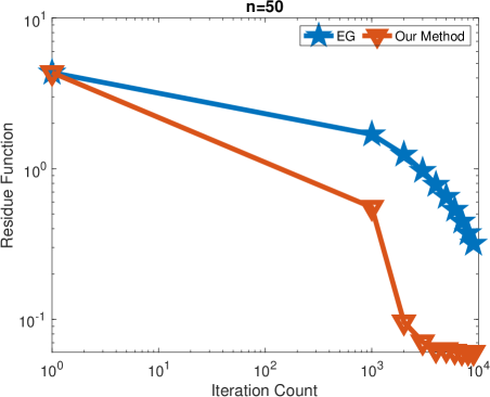
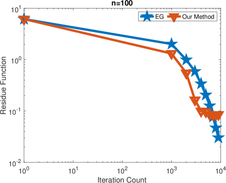
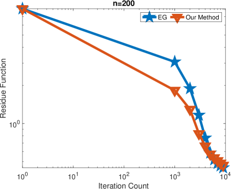
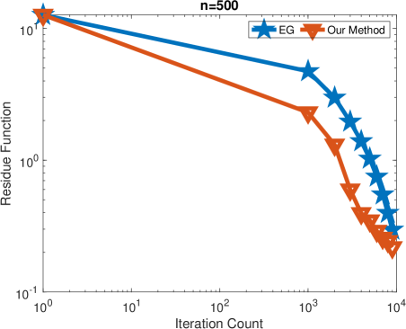
Figure 1: Performance of all the algorithms for $n\in\{50,100,200\}$ when $\rho=\frac{1}{20n}$ is set. The numerical results are presented in terms of iteration count (Top) and computational time (Bottom).

Following the setup of Jiang and Mokhtari (2022), we consider a problem in the following form:

$$\min_{z\in\mathbb{R}^{n}}\max_{y\in\mathbb{R}^{n}}\ f(z,y)=\tfrac{\rho}{24}\|z\|^{4}+y^{\top}(Az-b),$$ (5.1)

where $\rho>0$, the entries of $b\in\mathbb{R}^{n}$ are generated independently from $[-1,1]$ and $A\in\mathbb{R}^{n\times n}$ is given by

$$A=\begin{bmatrix}1&-1&&&\\ &1&-1&&\\ &&\ddots&\ddots&\\ &&&1&-1\\ &&&&1\end{bmatrix}.$$

This min-max optimization problem is convex-concave and has a unique global solution $z^{\star}=A^{-1}b$ and $y^{\star}=-\frac{\rho}{6}\|z^{\star}\|^{2}(A^{\top})^{-1}z^{\star}$. It can be reformulated in the form of ME problem (cf. Eq. (1.1)) with

$$x=\begin{bmatrix}z\\ y\end{bmatrix},\qquad F(x)=\begin{bmatrix}\tfrac{\rho}{6}\|z\|^{2}z+A^{\top}y\\ -(Az-b)\end{bmatrix}.$$

In our experiment, we set $\rho=\frac{1}{100n}$ where $n\in\{50,100,200,500\}$ varies and use the residue function as the evaluation metric. We set the stepsize in the EG method as $0.05$ and $p=3$ in Algorithm 2. Our results are summarized in Figure 1 and we can see that our new method outperforms the EG method in terms of solution accuracy. This is because that our method can exploit the special structure of Eq. (5.1), demonstrating the potential to design new gradient-based algorithms for solving structured application problems. Our empirical findings coincide with a line of existing works (Maddison et al., 2018; Zhang et al., 2018; Wilson et al., 2019; O’Donoghue and Maddison, 2019; Loizou et al., 2020), which designed new accelerated gradient-based methods for solving structured problems (e.g., with strongly smooth loss functions) with provably fast global convergence rate and favorable numerical results.

6 Conclusions

We have presented a new class of accelerated rescaled gradient systems that yield global acceleration in the general setting of monotone equation (ME) problems. Our analysis shows that our systems are equivalent to closed-loop control systems (Lin and Jordan, 2023), which allows for establishing desired properties of solution trajectories, including global existence and uniqueness, global asymptotic weak and/or strong convergence, and global convergence rate estimation in terms of a residue function. Our framework provides a systematic approach to deriving existing high-order methods and additionally to derive a new suite of simple first-order methods for solving ME problems. The same global rate in terms of a residue function is established for these methods under suitable high-order Lipschitz continuity conditions. For future research, it would be of interest to bring our continuous-time perspective for understanding various ME methods into register with the Lagrangian and Hamiltonian frameworks that have proved productive (Wibisono et al., 2016; Diakonikolas and Jordan, 2021; Muehlebach and Jordan, 2021).

References

- Abbas et al. [2014] B. Abbas, H. Attouch, and B. F. Svaiter. Newton-like dynamics and forward-backward methods for structured monotone inclusions in Hilbert spaces. Journal of Optimization Theory and Applications, 161(2):331–360, 2014.
- Adil et al. [2022] D. Adil, B. Bullins, A. Jambulapati, and S. Sachdeva. Optimal methods for higher-order smooth monotone variational inequalities. ArXiv Preprint: 2205.06167, 2022.
- Ambrosio et al. [2005] L. Ambrosio, N. Gigli, and G. Savaré. Gradient Flows: in Metric Spaces and in the Space of Probability Measures. Springer Science & Business Media, 2005.
- Arscott and Filippov [1988] F. M. Arscott and A. F. Filippov. Differential Equations with Discontinuous Righthand Sides: Control Systems. Springer Netherlands, 1988.
- Attouch and László [2020] H. Attouch and S. C. László. Newton-like inertial dynamics and proximal algorithms governed by maximally monotone operators. SIAM Journal on Optimization, 30(4):3252–3283, 2020.
- Attouch and László [2021] H. Attouch and S. C. László. Continuous Newton-like inertial dynamics for monotone inclusions. Set-Valued and Variational Analysis, 29(3):555–581, 2021.
- Attouch and Svaiter [2011] H. Attouch and B. F. Svaiter. A continuous dynamical Newton-like approach to solving monotone inclusions. SIAM Journal on Control and Optimization, 49(2):574–598, 2011.
- Attouch et al. [2013] H. Attouch, P. Redont, and B. F. Svaiter. Global convergence of a closed-loop regularized Newton method for solving monotone inclusions in Hilbert spaces. Journal of Optimization Theory and Applications, 157(3):624–650, 2013.
- Attouch et al. [2016a] H. Attouch, M. M. Alves, and B. F. Svaiter. A dynamic approach to a proximal-Newton method for monotone inclusions in Hilbert spaces, with complexity . Journal of Convex Analysis, 23(1):139–180, 2016a.
- Attouch et al. [2016b] H. Attouch, J. Peypouquet, and P. Redont. Fast convex optimization via inertial dynamics with Hessian driven damping. Journal of Differential Equations, 261(10):5734–5783, 2016b.
- Attouch et al. [2018] H. Attouch, Z. Chbani, J. Peypouquet, and P. Redont. Fast convergence of inertial dynamics and algorithms with asymptotic vanishing viscosity. Mathematical Programming, 168(1-2):123–175, 2018.
- Bauschke and Combettes [2001] H. H. Bauschke and P. L. Combettes. A weak-to-strong convergence principle for Fejér-monotone methods in Hilbert spaces. Mathematics of Operations Research, 26(2):248–264, 2001.
- Benaïm and Hirsch [1996] M. Benaïm and M. W. Hirsch. Asymptotic pseudotrajectories and chain recurrent flows, with applications. Journal of Dynamics and Differential Equations, 8:141–176, 1996.
- Benaïm et al. [2005] M. Benaïm, J. Hofbauer, and S. Sorin. Stochastic approximations and differential inclusions. SIAM Journal on Control and Optimization, 44(1):328–348, 2005.
- Bertsekas [1982] D. P. Bertsekas. Constrained Optimization and Lagrange Multiplier Methods. Academic Press, 1982.
- Bruck Jr [1977] R. E. Bruck Jr. On the weak convergence of an ergodic iteration for the solution of variational inequalities for monotone operators in Hilbert space. Journal of Mathematical Analysis and Applications, 61(1):159–164, 1977.
- Bullins and Lai [2022] B. Bullins and K. A. Lai. Higher-order methods for convex-concave min-max optimization and monotone variational inequalities. SIAM Journal on Optimization, 32(3):2208–2229, 2022.
- Cai et al. [2022] Y. Cai, A. Oikonomou, and W. Zheng. Finite-time last-iterate convergence for learning in multi-player games. In NeurIPS, pages 33904–33919, 2022.
- Cesa-Bianchi and Lugosi [2006] N. Cesa-Bianchi and G. Lugosi. Prediction, Learning, and Games. Cambridge University Press, 2006.
- Cordero and Torregrosa [2007] A. Cordero and J. R. Torregrosa. Variants of Newton’s method using fifth-order quadrature formulas. Applied Mathematics and Computation, 190(1):686–698, 2007.
- Cortés [2006] J. Cortés. Finite-time convergent gradient flows with applications to network consensus. Automatica, 42(11):1993–2000, 2006.
- Courant [1943] R. Courant. Variational methods for the solution of problems of equilibrium and vibrations. Bulletin of the American Mathematical Society, 49(1):1–23, 1943.
- Darvishi and Barati [2007] M. T. Darvishi and A. Barati. A third-order Newton-type method to solve systems of nonlinear equations. Applied Mathematics and Computation, 187(2):630–635, 2007.
- Diakonikolas and Jordan [2021] J. Diakonikolas and M. I. Jordan. Generalized momentum-based methods: A Hamiltonian perspective. SIAM Journal on Optimization, 31(1):915–944, 2021.
- Diakonikolas and Orecchia [2019] J. Diakonikolas and L. Orecchia. The approximate duality gap technique: A unified theory of first-order methods. SIAM Journal on Optimization, 29(1):660–689, 2019.
- Esfahani and Kuhn [2018] P. M. Esfahani and D. Kuhn. Data-driven distributionally robust optimization using the Wasserstein metric: Performance guarantees and tractable reformulations. Mathematical Programming, 171(1):115–166, 2018.
- Facchinei and Pang [2007] Francisco Facchinei and Jong-Shi Pang. Finite-Dimensional Variational Inequalities and Complementarity Problems. Springer Science & Business Media, 2007.
- Filippov [1964] A. F. Filippov. Differential equations with discontinuous right-hand side. American Mathematical Society Translations, 42:199–231, 1964.
- Fudenberg and Levine [1998] D. Fudenberg and D. K. Levine. The Theory of Learning in Games, volume 2. MIT Press, 1998.
- Golowich et al. [2020a] N. Golowich, S. Pattathil, and C. Daskalakis. Tight last-iterate convergence rates for no-regret learning in multi-player games. In NeurIPS, pages 20766–20778, 2020a.
- Golowich et al. [2020b] N. Golowich, S. Pattathil, C. Daskalakis, and A. Ozdaglar. Last iterate is slower than averaged iterate in smooth convex-concave saddle point problems. In COLT, pages 1758–1784. PMLR, 2020b.
- Goodfellow et al. [2020] I. Goodfellow, J. Pouget-Abadie, M. Mirza, B. Xu, D. Warde-Farley, S. Ozair, A. Courville, and Y. Bengio. Generative adversarial networks. Communications of the ACM, 63(11):139–144, 2020.
- Gorbunov et al. [2022] E. Gorbunov, N. Loizou, and G. Gidel. Extragradient method: O (1/k) last-iterate convergence for monotone variational inequalities and connections with cocoercivity. In AISTATS, pages 366–402. PMLR, 2022.
- Güler [1991] O. Güler. On the convergence of the proximal point algorithm for convex minimization. SIAM Journal on Control and Optimization, 29(2):403–419, 1991.
- Hadamard [1908] J. Hadamard. Mémoire sur le problème d’analyse relatif à l’équilibre des plaques élastiques encastrées, volume 33. Imprimerie Nationale, 1908.
- Hammond and Magnanti [1987] J. H. Hammond and T. L. Magnanti. Generalized descent methods for asymmetric systems of equations. Mathematics of Operations Research, 12(4):678–699, 1987.
- Heath [2018] M. T. Heath. Scientific Computing: An Introductory Survey, Revised Second Edition. SIAM, 2018.
- Homeier [2004] H. H. H. Homeier. A modified Newton method with cubic convergence: the multivariate case. Journal of Computational and Applied Mathematics, 169(1):161–169, 2004.
- Jiang and Mokhtari [2022] R. Jiang and A. Mokhtari. Generalized optimistic methods for convex-concave saddle point problems. ArXiv Preprint: 2202.09674, 2022.
- Kelley [1995] C. T. Kelley. Iterative Methods for Linear and Nonlinear Equations. SIAM, 1995.
- Kelley [2003] C. T. Kelley. Solving Nonlinear Equations with Newton’s Method. SIAM, 2003.
- Korpelevich [1976] G. M. Korpelevich. The extragradient method for finding saddle points and other problems. Matecon, 12:747–756, 1976.
- Kotsalis et al. [2022] G. Kotsalis, G. Lan, and T. Li. Simple and optimal methods for stochastic variational inequalities, I: operator extrapolation. SIAM Journal on Optimization, 32(3):2041–2073, 2022.
- Lin and Jordan [2022a] T. Lin and M. I. Jordan. A control-theoretic perspective on optimal high-order optimization. Mathematical Programming, 195(1):929–975, 2022a.
- Lin and Jordan [2022b] T. Lin and M. I. Jordan. Perseus: A simple and optimal high-order method for variational inequalities. ArXiv Preprint: 2205.03202, 2022b.
- Lin and Jordan [2023] T. Lin and M. I. Jordan. Monotone inclusions, acceleration, and closed-loop control. Mathematics of Operations Research, 48(4):2353–2382, 2023.
- Lin et al. [2020] T. Lin, Z. Zhou, P. Mertikopoulos, and M. I. Jordan. Finite-time last-iterate convergence for multi-agent learning in games. In ICML, pages 6161–6171, 2020.
- Lin et al. [2021] T. Lin, Z. Zhou, W. Ba, and J. Zhang. Doubly optimal no-regret online learning in strongly monotone games with bandit feedback. ArXiv Preprint: 2112.02856, 2021.
- Lin et al. [2022] T. Lin, P. Mertikopoulos, and M. I. Jordan. Explicit second-order min-max optimization methods with optimal convergence guarantee. ArXiv Preprint: 2210.12860, 2022.
- Lions [1978] P. L. Lions. Une méthode itérative de résolution d’une inéquation variationnelle. Israel Journal of Mathematics, 31(2):204–208, 1978.
- Loizou et al. [2020] N. Loizou, H. Berard, A. Jolicoeur-Martineau, P. Vincent, S. Lacoste-Julien, and I. Mitliagkas. Stochastic Hamiltonian gradient methods for smooth games. In ICML, pages 6370–6381, 2020.
- Maddison et al. [2018] C. J. Maddison, D. Paulin, Y. W. Teh, B. O’Donoghue, and A. Doucet. Hamiltonian descent methods. ArXiv Preprint: 1809.05042, 2018.
- Magnanti and Perakis [1997] T. L. Magnanti and G. Perakis. Averaging schemes for variational inequalities and systems of equations. Mathematics of Operations Research, 22(3):568–587, 1997.
- Maingé [2013] P-E. Maingé. First-order continuous Newton-like systems for monotone inclusions. SIAM Journal on Control and Optimization, 51(2):1615–1638, 2013.
- McDougall and Wotherspoon [2014] T. J. McDougall and S. J. Wotherspoon. A simple modification of Newton’s method to achieve convergence of order 1+. Applied Mathematics Letters, 29:20–25, 2014.
- Meintjes and Morgan [1990] K. Meintjes and A. P. Morgan. Chemical equilibrium systems as numerical test problems. ACM Transactions on Mathematical Software (TOMS), 16(2):143–151, 1990.
- Mertikopoulos and Staudigl [2018] P. Mertikopoulos and M. Staudigl. Stochastic mirror descent dynamics and their convergence in monotone variational inequalities. Journal of Optimization Theory and Applications, 179(3):838–867, 2018.
- Mertikopoulos and Zhou [2019] P. Mertikopoulos and Z. Zhou. Learning in games with continuous action sets and unknown payoff functions. Mathematical Programming, 173:465–507, 2019.
- Mertikopoulos et al. [2018] P. Mertikopoulos, C. Papadimitriou, and G. Piliouras. Cycles in adversarial regularized learning. In SODA, pages 2703–2717. SIAM, 2018.
- Mokhtari et al. [2020] A. Mokhtari, A. E. Ozdaglar, and S. Pattathil. Convergence rate of o(1/k) for optimistic gradient and extragradient methods in smooth convex-concave saddle point problems. SIAM Journal on Optimization, 30(4):3230–3251, 2020.
- Monteiro and Svaiter [2010] R. D. C. Monteiro and B. F. Svaiter. On the complexity of the hybrid proximal extragradient method for the iterates and the ergodic mean. SIAM Journal on Optimization, 20(6):2755–2787, 2010.
- Monteiro and Svaiter [2011] R. D. C. Monteiro and B. F. Svaiter. Complexity of variants of Tseng’s modified FB splitting and Korpelevich’s methods for hemivariational inequalities with applications to saddle-point and convex optimization problems. SIAM Journal on Optimization, 21(4):1688–1720, 2011.
- Monteiro and Svaiter [2012] R. D. C. Monteiro and B. F. Svaiter. Iteration-complexity of a Newton proximal extragradient method for monotone variational inequalities and inclusion problems. SIAM Journal on Optimization, 22(3):914–935, 2012.
- Moore [1979] R. E. Moore. Methods and Applications of Interval Analysis. SIAM, 1979.
- Morgan [2009] A. Morgan. Solving polynomial systems using continuation for engineering and scientific problems. SIAM, 2009.
- Morgan and Sommese [1987] A. Morgan and A. Sommese. Computing all solutions to polynomial systems using homotopy continuation. Applied Mathematics and Computation, 24(2):115–138, 1987.
- Morgenstern and Von Neumann [1953] O. Morgenstern and J. Von Neumann. Theory of Games and Economic Behavior. Princeton University Press, 1953.
- Muehlebach and Jordan [2019] M. Muehlebach and M. I. Jordan. A dynamical systems perspective on Nesterov acceleration. In ICML, pages 4656–4662, 2019.
- Muehlebach and Jordan [2021] M. Muehlebach and M. I. Jordan. Optimization with momentum: Dynamical, control-theoretic, and symplectic perspectives. Journal of Machine Learning Research, 22(73):1–50, 2021.
- Muehlebach and Jordan [2022] M. Muehlebach and M. I. Jordan. On constraints in first-order optimization: A view from non-smooth dynamical systems. Journal of Machine Learning Research, 23(256):1–47, 2022.
- Nemirovski [2004] A. Nemirovski. Prox-method with rate of convergence o(1/t) for variational inequalities with Lipschitz continuous monotone operators and smooth convex-concave saddle point problems. SIAM Journal on Optimization, 15(1):229–251, 2004.
- Nemirovski [1981] A. S. Nemirovski. Effective iterative methods for solving equations with monotone operators. Ekonom. i Mat. Metody, 17(2):344–359, 1981.
- Nemirovski and Yudin [1978] A. S. Nemirovski and D. B. Yudin. Cesari convergence of the gradient method of approximating saddle points of convex-concave functions. Doklady Akademii Nauk, 239(5):1056–1059, 1978.
- Nesterov [2007] Y. Nesterov. Dual extrapolation and its applications to solving variational inequalities and related problems. Mathematical Programming, 109(2):319–344, 2007.
- O’Donoghue and Maddison [2019] B. O’Donoghue and C. J. Maddison. Hamiltonian descent for composite objectives. In NeurIPS, pages 14470–14480, 2019.
- Ouyang and Xu [2021] Y. Ouyang and Y. Xu. Lower complexity bounds of first-order methods for convex-concave bilinear saddle-point problems. Mathematical Programming, 185(1):1–35, 2021.
- O’donoghue and Candes [2015] B. O’donoghue and E. Candes. Adaptive restart for accelerated gradient schemes. Foundations of Computational Mathematics, 15(3):715–732, 2015.
- Paden and Sastry [1987] B. Paden and S. Sastry. A calculus for computing Filippov’s differential inclusion with application to the variable structure control of robot manipulators. IEEE Transactions on Circuits and Systems, 34(1):73–82, 1987.
- Popov [1980] L. D. Popov. A modification of the Arrow-Hurwicz method for search of saddle points. Mathematical notes of the Academy of Sciences of the USSR, 28(5):845–848, 1980.
- Romero and Benosman [2020] O. Romero and M. Benosman. Finite-time convergence in continuous-time optimization. In ICML, pages 8200–8209. PMLR, 2020.
- Roulet and d’Aspremont [2017] V. Roulet and A. d’Aspremont. Sharpness, restart and acceleration. In NeurIPS, pages 1119–1129, 2017.
- Ryu et al. [2019] E. K. Ryu, K. Yuan, and W. Yin. ODE analysis of stochastic gradient methods with optimism and anchoring for minimax problems. ArXiv Preprint: 1905.10899, 2019.
- Schropp [1995] J. Schropp. Using dynamical systems methods to solve minimization problems. Applied Numerical Mathematics, 18(1-3):321–335, 1995.
- Schropp and Singer [2000] J. Schropp and I. Singer. A dynamical systems approach to constrained minimization. Numerical Functional Analysis and Optimization, 21(3-4):537–551, 2000.
- Shamma [2008] J. Shamma. Cooperative Control of Distributed Multi-agent Systems. John Wiley & Sons, 2008.
- Shi et al. [2022] B. Shi, S. S. Du, M. I. Jordan, and W. J. Su. Understanding the acceleration phenomenon via high-resolution differential equations. Mathematical Programming, 195(1):79–148, 2022.
- Solodov and Svaiter [1999a] M. V. Solodov and B. F. Svaiter. A globally convergent inexact Newton method for systems of monotone equations. Reformulation: Nonsmooth, Piecewise Smooth, Semismooth and Smoothing Methods, pages 355–369, 1999a.
- Solodov and Svaiter [1999b] M. V. Solodov and B. F. Svaiter. A hybrid approximate extragradient-proximal point algorithm using the enlargement of a maximal monotone operator. Set-Valued Analysis, 7(4):323–345, 1999b.
- Su et al. [2016] W. Su, S. Boyd, and E. J. Candès. A differential equation for modeling Nesterov’s accelerated gradient method: theory and insights. The Journal of Machine Learning Research, 17(1):5312–5354, 2016.
- Verschelde et al. [1994] J. Verschelde, P. Verlinden, and R. Cools. Homotopies exploiting Newton polytopes for solving sparse polynomial systems. SIAM Journal on Numerical Analysis, 31(3):915–930, 1994.
- Wibisono et al. [2016] A. Wibisono, A. C. Wilson, and M. I. Jordan. A variational perspective on accelerated methods in optimization. Proceedings of the National Academy of Sciences, 113(47):E7351–E7358, 2016.
- Wilson et al. [2019] A. C. Wilson, L. Mackey, and A. Wibisono. Accelerating rescaled gradient descent: Fast optimization of smooth functions. In NeurIPS, pages 13555–13565, 2019.
- Wilson et al. [2021] A. C. Wilson, B. Recht, and M. I. Jordan. A Lyapunov analysis of accelerated methods in optimization. Journal of Machine Learning Research, 22(113):1–34, 2021.
- Xu et al. [2009] H. Xu, C. Caramanis, and S. Mannor. Robustness and regularization of support vector machines. Journal of Machine Learning Research, 10(Jul):1485–1510, 2009.
- Yoon and Ryu [2021] T. Yoon and E. K. Ryu. Accelerated algorithms for smooth convex-concave minimax problems with rate on squared gradient norm. In ICML, pages 12098–12109. PMLR, 2021.
- Zhang et al. [2018] J. Zhang, A. Mokhtari, S. Sra, and A. Jadbabaie. Direct Runge-Kutta discretization achieves acceleration. In NIPS, pages 3904–3913, 2018.
- Zhou et al. [2017] Z. Zhou, P. Mertikopoulos, A. L. Moustakas, N. Bambos, and P. Glynn. Mirror descent learning in continuous games. In CDC, pages 5776–5783. IEEE, 2017.
- Zhou et al. [2020] Z. Zhou, P. Mertikopoulos, N. Bambos, S. P. Boyd, and P. W. Glynn. On the convergence of mirror descent beyond stochastic convex programming. SIAM Journal on Optimization, 30(1):687–716, 2020.