QuasinormalModes.jl: A Julia package for computing discrete eigenvalues of second order ODEs

Summary

In General Relativity, when perturbing a black hole with an external field, or particle, the system relaxes by emitting damped gravitational waves, known as quasinormal modes. These are the characteristic frequencies of the black hole and gain the quasi prefix due to the fact that they have a real frequency, which represents the oscillation frequency of the response, and an imaginary frequency that represents the decay rate of said oscillations. In many cases, such perturbations can be described by a second order homogeneous ordinary differential equation (ODE) with discrete complex eigenvalues.

Determining these characteristic frequencies quickly and accurately for a large range of models is important for many practical reasons. It has been shown that the gravitational wave signal emitted at the final stage of the coalescence of two compact objects is well described by quasinormal modes (Buonanno et al., 2007; Seidel, 2004). This means that if one has access to a database of quasinormal modes and of gravitational wave signals from astrophysical collision events, it is possible to characterize the remnant object using its quasinormal frequencies. Since there are many different models that aim to describe remnants, being able to compute the quasinormal frequencies for such models in a reliable way is paramount for confirming or discarding them.

Statement of need

QuasinormalModes.jl is a Julia package for computing the quasinormal modes of any General Relativity model whose perturbation equation can be expressed as second order homogeneous ODE. Not only that, the package can be used to compute the discrete eigenvalues of any second order homogeneous ODE (such as the energy eigenstates of the time independent Schrödinger equation) provided that these eigenvalues actually exist. The package features a flexible and user friendly API where the user simply needs to provide the coefficients of the problem ODE after incorporating boundary and asymptotic conditions on it. The user can also choose to use machine or arbitrary precision arithmetic for the underlying floating point operations involved and whether or not to do computations sequentially or in parallel using threads. The API also tries not to force any particular workflow on the users so that they can incorporate and adapt the existing functionality on their research pipelines without unwanted intrusions. Often user friendliness, flexibility and performance are treated as mutually exclusive, particularly in scientific applications. By using Julia as an implementation language, the package can have all of theses features simultaneously.

Another important motivation for using Julia and writing this package was the lack of generalist, free (both in the financial and license-wise sense) open source tools that serve the same purpose. More precisely, there are tools which are free and open source, but run on top of a proprietary paid and expensive software framework such as the ones developped by Jansen (2017) and Fortuna & Vega (2020), which are both excellent packages that aim to perform the same task as QuasinormalModes.jl and can be obtained and modified freely but, unfortunately, require the user to own a license of the proprietary Wolfram Mathematica CAS. Furthermore, their implementations are limited to solve problems where the eigenvalues must appear in the ODE as a polynomials of order $p$. While this is not prohibitively restrictive to most astrophysics problems, it can be an important limitation in other areas. There are also packages that are free and run on top of Mathematica but are not aimed at being general eigenvalue solvers at all, such as the one by O’Toole et al. (2019), that can only compute modes of Schwarzschild and Kerr black holes. Finally, the Python package by Stein (2019) is open source and free but can only compute Kerr quasinormal modes.

QuasinormalModes.jl fills the existing gap for free, open source tools that are able to compute discrete eigenvalues (and in particular, quasinormal modes) efficiently for a broad class of models and problems. The package was developed during the author’s PhD research where it is actively used for producing novel results that shall appear in the author’s thesis. It is also actively used in a collaborative research effort (of which the author is one of the members) for computing quasinormal modes produced by perturbations with integer (but different than 0) spins and semi-integer spins. These results are being contrasted with those obtained by other methods and so far show excellent agreement with each other and with literature results.

Underlying algorithm

QuasinormalModes.jl internally uses a relativity new numerical method called the Asymptotic Iteration Method (AIM). The method was introduced by Ciftci et al. (2003) but the actual implementation used in this package is based on the revision performed by Cho et al. (2012). The main purpose of the (AIM) is to solve the following general linear homogeneous second order ODE:

$$y^{\prime\prime}(x)-\lambda_{0}(x)y^{\prime}(x)-s_{0}(x)y(x)=0,$$ (1)

where primes denote derivatives with respect to to the variable $x$ (that is defined over some interval that is not necessarily bounded), $\lambda_{0}(x)\neq 0$ and $s_{0}(x)\in C_{\infty}$. The method is based upon the following theorem: let $\lambda_{0}$ and $s_{0}$ be functions of the variable $x\in(a,b)$ that are $C_{\infty}$ on the same interval, the solution of the differential equation, Eq. (1), has the form

$$y(x)=\exp\left(-\int\alpha\mathrm{d}t\right)\times\left[C_{2}+C_{1}\int^{x}\exp\left(\int^{t}(\lambda_{0}(\tau)+2\alpha(\tau))\mathrm{d}\tau\right)\mathrm{d}t\right]$$ (2)

if for some $n>0$ the condition

$$\delta\equiv s_{n}\lambda_{n-1}-\lambda_{n}s_{n-1}=0$$ (3)

is satisfied, where

$$\lambda_{k}(x)\equiv \lambda^{\prime}_{k-1}(x)+s_{k-1}(x)+\lambda_{0}(x)\lambda_{k-1}(x)$$ (4)

$$s_{k}(x)\equiv s^{\prime}_{k-1}(x)+s_{0}\lambda_{k-1}(x)$$ (5)

where $k$ is an integer that ranges from $1$ to $n$.

Provided that the theorem is satisfied we can find both the eigenvalues and eigenvectors of the second order ODE using, respectively, Eq. (3) and Eq. (2). Due to the recursive nature of Eq.(4) and Eq.(5), to compute the quantization condition, Eq.(3), using $n$ iterations the $n$-th derivatives of $\lambda_{0}$ and $s_{0}$ must be computed multiple times. To address this issue, Cho et al. (2012) proposed the use of a Taylor expansion of both $\lambda$ and $s$ around a point $\xi$ where the AIM is to be performed. This improved version is implemented in QuasinormalModes.jl

Benchmark

To show QuasinormalModes.jl in action, this section provides a simple benchmark where the fundamental quasinormal mode ($n=\ell=m=s=0$) of a Schwarzschild black hole was computed using 16 threads on a Intel(R) Core(TM) i9-7900X @ 3.30GHz CPU with 256 bit precision floating point numbers.

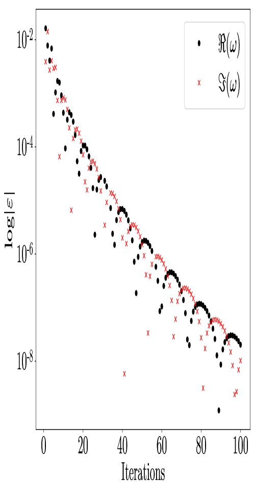
Figure 1: Error convergence for the fundamental Schwarzschild quasinormal mode as a function of the number of AIM iterations.

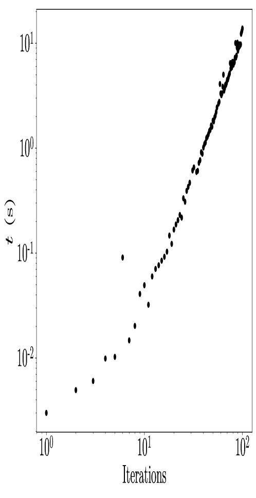
Figure 2: Time taken to compute the fundamental Schwarzschild quasinormal mode as a function of the number of AIM iterations on a logarithmic scale.

In order to quantify the rate at which the method converges to the correct results, the error measure $\varepsilon$ was defined as follows: given the computed real and imaginary quasinormal frequencies, denoted respectively by $\omega_{R}$ and $\omega_{I}$, and the reference frequencies given by Berti et al. (2009), denoted respectively as $\overline{\omega}_{R}$ and $\overline{\omega}_{I}$ we have that $|\varepsilon|=|\omega_{R,I}-\overline{\omega}_{R,I}|$. In Figure 1 $\varepsilon$ is plotted as a function of the number of iterations for both the real and imaginary frequencies. We can see that, as the number of iterations increases, the error in the computed values rapidly decreases.

In Figure 2, the time required to perform a certain number of iterations is plotted in logarithmic scale. Each data point is the arithmetic mean time obtained after 10 runs of the algorithm for a given number of iterations. The time measurement takes care to exclude the overhead induced at “startup” due to Julia’s JIT compilation. Even though the time taken to perform a certain number of iterations increases with a power law, the time scale required to achieve highly accurate results is still around 10s. This time would be even smaller if one choose to use built-in floating point types instead of arbitrary precision numbers.

References

Berti, E., Cardoso, V., & Starinets, A. O. (2009). Quasinormal modes of black holes and black branes. Class. Quant. Grav., 26, 163001. https://doi.org/10.1088/0264-9381/26/16/163001

Buonanno, A., Cook, G. B., & Pretorius, F. (2007). Inspiral, merger and ring-down of equal-mass black-hole binaries. Phys. Rev. D, 75, 124018. https://doi.org/10.1103/PhysRevD.75.124018

Cho, H. T., Cornell, A. S., Doukas, J., Huang, T. R., & Naylor, W. (2012). A New Approach to Black Hole Quasinormal Modes: A Review of the Asymptotic Iteration Method. Adv. Math. Phys., 2012, 281705. https://doi.org/10.1155/2012/281705

Ciftci, H., Hall, R. L., & Saad, N. (2003). Asymptotic iteration method for eigenvalue problems. Journal of Physics A: Mathematical and General, 36(47), 11807–11816. https://doi.org/10.1088/0305-4470/36/47/008

Fortuna, S., & Vega, I. (2020). Bernstein spectral method for quasinormal modes and other eigenvalue problems. http://arxiv.org/abs/2003.06232

Jansen, A. (2017). Overdamped modes in Schwarzschild-de Sitter and a Mathematica package for the numerical computation of quasinormal modes. Eur. Phys. J. Plus, 132(12), 546. https://doi.org/10.1140/epjp/i2017-11825-9

O’Toole, C., Macedo, R., Stratton, T., & Wardell, B. (2019). QuasiNormalModes. In GitHub repository. GitHub. https://github.com/BlackHolePerturbationToolkit/QuasiNormalModes

Seidel, E. (2004). Nonlinear impact of perturbation theory on numerical relativity. Classical and Quantum Gravity, 21(3), S339–S349. https://doi.org/10.1088/0264-9381/21/3/021

Stein, L. C. (2019). qnm: A Python package for calculating Kerr quasinormal modes, separation constants, and spherical-spheroidal mixing coefficients. Journal of Open Source Software, 4(42), 1683. https://doi.org/10.21105/joss.01683