I’m Me, We’re Us, and I’m Us:
Tri-directional Contrastive Learning on Hypergraphs

Abstract

Although machine learning on hypergraphs has attracted considerable attention, most of the works have focused on (semi-)supervised learning, which may cause heavy labeling costs and poor generalization. Recently, contrastive learning has emerged as a successful unsupervised representation learning method. Despite the prosperous development of contrastive learning in other domains, contrastive learning on hypergraphs remains little explored. In this paper, we propose TriCL (Tri-directional Contrastive Learning), a general framework for contrastive learning on hypergraphs. Its main idea is tri-directional contrast, and specifically, it aims to maximize in two augmented views the agreement (a) between the same node, (b) between the same group of nodes, and (c) between each group and its members. Together with simple but surprisingly effective data augmentation and negative sampling schemes, these three forms of contrast enable TriCL to capture both node- and group-level structural information in node embeddings. Our extensive experiments using 14 baseline approaches, 10 datasets, and two tasks demonstrate the effectiveness of TriCL, and most noticeably, TriCL almost consistently outperforms not just unsupervised competitors but also (semi-)supervised competitors mostly by significant margins for node classification. The code and datasets are available at https://github.com/wooner49/TriCL.

1 Introduction

Many real-world interactions are group-wise. Examples include collaborations of researchers, discussions on online Q&A sites, group conversations on messaging apps, co-citations of documents, and co-purchases of items. A hypergraph, which is a generalized graph, allows an edge to join an arbitrary number of nodes, and thus each such edge, which is called a hyperedge, naturally represents such group-wise interactions (Benson et al. 2018; Do et al. 2020; Lee, Ko, and Shin 2020).

Recently, machine learning on hypergraphs has drawn a lot of attention from a broad range of fields, including social network analysis (Yang et al. 2019), recommender systems (Xia et al. 2021), and bioinformatics (Zheng et al. 2019). Hypergraph-based approaches often outperform graph-based ones on various machine learning tasks, including classification (Feng et al. 2019), clustering (Benson, Gleich, and Leskovec 2016), ranking (Yu et al. 2021), and outlier detection (Lee, Choe, and Shin 2022).

Previous studies have largely focused on developing encoder architectures so-called hypergraph neural networks for hypergraph-structured data (Feng et al. 2019; Yadati et al. 2019; Dong, Sawin, and Bengio 2020; Bai, Zhang, and Torr 2021; Arya et al. 2020), and in most cases, such hypergraph neural networks are trained in a (semi-)supervised way. However, data labeling is often time, resource, and labor-intensive, and neural networks trained only in a supervised way can easily overfit and may fail to generalize (Rong et al. 2020), making it difficult to be applied to other tasks.

Thus, self-supervised learning (Liu et al. 2022; Jaiswal et al. 2020; Liu et al. 2021), which does not require labels, has become popular, and especially contrastive learning has achieved great success in computer vision (Chen et al. 2020; Hjelm et al. 2019) and natural language processing  (Gao, Yao, and Chen 2021). Contrastive learning has proved effective also for learning on (ordinary) graphs (Veličković et al. 2018b; Peng et al. 2020; Hassani and Khasahmadi 2020; Zhu et al. 2020, 2021b; You et al. 2020), and a common approach is to (a) create two augmented views from the input graph and (b) learn machine learning models to maximize the agreement between the two views.

However, contrastive learning on hypergraphs remains largely underexplored with only a handful of previous studies (Xia et al. 2021; Zhang et al. 2021; Yu et al. 2021) (see Section 2 for details). Especially, the following questions remain open: (Q1) what to contrast?, (Q2) how to augment a hypergraph?, and (Q3) how to select negative samples?

For Q1, which is our main focus, we propose tri-directional contrast. In addition to node-level contrast, which is the only form of contrast employed in the previous studies, we propose the use of group-level and membership-level contrast. That is, in two augmented views, we aim to maximize agreements (a) between the same node, (b) between the same group of nodes, and (c) between each group and its members. These three forms of contrast are complementary, leading to representations that capture both node- and group-level (i.e., higher-order) relations in hypergraphs.

In addition, for Q2, we demonstrate that combining two simple augmentation strategies (spec., membership corruption and feature corruption) is effective. For Q3, we reveal that uniform random sampling is surprisingly successful, and in our experiments, even an extremely small sample size leads to marginal performance degradation.

Our proposed method TriCL, which is based on the aforementioned observations, is evaluated extensively using 14 baseline approaches, 10 datasets, and two tasks. The most notable result is that, for node classification, TriCL outperforms not just unsupervised competitors but also all (semi-)supervised competitors on almost all considered datasets, mostly by considerable margins. Moreover, we demonstrate the consistent effectiveness of tri-directional contrast, which is our main contribution.

2 Related Work

Hypergraph learning

Due to its enough expressiveness to capture higher-order structural information, learning on hypergraphs has received a lot of attention. Many recent studies have focused on generalizing graph neural networks (GNNs) to hypergraphs (Feng et al. 2019; Bai, Zhang, and Torr 2021; Yadati et al. 2019). Most of them redefine hypergraph message aggregation schemes based on clique expansion (i.e., replacing hyperedges with cliques to obtain a graph) or its variants. While its simplicity is appealing, clique expansion causes structural distortion and leads to undesired information loss (Hein et al. 2013; Li and Milenkovic 2018). On the other hand, HNHN (Dong, Sawin, and Bengio 2020) prevents information loss by extending star expansion using two distinct weight matrices for node- and hyperedge-side message aggregations. Arya et al. (2020) propose HyperSAGE for inductive learning on hypergraphs based on two-stage message aggregation. Several studies attempt to unify hypergraphs and GNNs (Huang and Yang 2021; Zhang et al. 2022); and Chien et al. (2022) generalize message aggregation methods as multiset functions learned by Deep Sets (Zaheer et al. 2017) and Set Transformer (Lee et al. 2019). Most approaches above use (semi-)supervised learning.

Contrastive learning

In the image domain, the latest contrastive learning frameworks (e.g., SimCLR (Chen et al. 2020) and MoCo (He et al. 2020)) leverage the unchanging semantics under various image transformations, such as random flip, rotation, color distortion, etc, to learn visual features. They aim to learn distinguishable representations by contrasting positive and negative pairs.

In the graph domain, DGI (Veličković et al. 2018b) combines the power of GNNs and contrastive learning, which seeks to maximize the mutual information between node embeddings and graph embeddings. Recently, a number of graph contrastive learning approaches (You et al. 2020; Zhu et al. 2020, 2021b; Hassani and Khasahmadi 2020) that follow a common framework (Chen et al. 2020) have been proposed. Although these methods have achieved state-of-the-art performance on their task of interest, they cannot naturally exploit group-wise interactions, which we focus on in this paper. More recently, gCooL (Li, Jing, and Tong 2022) utilizes community contrast, which is a similar concept to membership-level contrast in TriCL, to maximize community consistency between two augmented views. However, gCooL has an information loss when constructing a community, thus information on subgroups (i.e., a smaller group in a large community) cannot be used. On the other hand, TriCL can preserve and fully utilize such group information.

Hypergraph contrastive learning

Contrastive learning on hypergraphs is still in its infancy. Recently, several studies explore contrastive learning on hypergraphs (Zhang et al. 2021; Xia et al. 2021; Yu et al. 2021). For example, Zhang et al. (2021) proposes S²-HHGR for group recommendation, which applies contrastive learning to remedy a data sparsity issue. In particular, they propose a hypergraph augmentation scheme that uses a coarse- and fine-grained node dropout for each view. However, they do not consider group-wise contrast. Although Xia et al. (2021) employ group-wise contrast for session recommendation, they do not account for node-wise and node-group pair-wise relationships when constructing their contrastive loss. Moreover, these approaches have been considered only in the context of group-based recommendation but not in the context of general representation learning.

3 Proposed Method: TriCL

In this section, we describe TriCL, our proposed framework for hypergraph contrastive learning. First, we introduce some preliminaries on hypergraphs and hypergraph neural networks, and then we elucidate the problem setting and details of the proposed method.

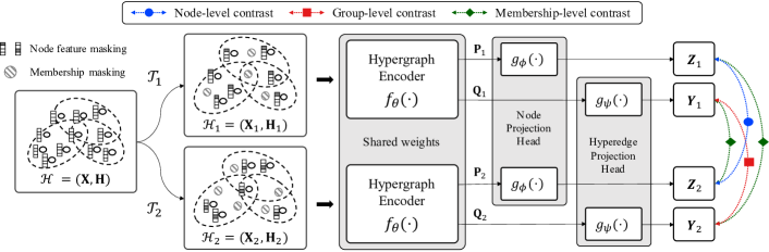
Figure 1: Overview of our proposed TriCL method. First, two different semantically similar views are generated by augmentations $\mathcal{T}_{1}$ and $\mathcal{T}_{2}$ from the original hypergraph. From these, we use a shared hypergraph encoder $f_{\theta}(\cdot)$ to form node and hyperedge representations. After passing node and hyperedge representations to their respective projection heads (i.e., $g_{\phi}(\cdot)$ and $g_{\psi}(\cdot)$), we maximize the agreement between two views via our proposed tri-directional contrast, which is a combination of node-, group-, and membership-level contrast.

3.1 Preliminaries

Hypergraphs and notation.

A hypergraph, a set of hyperedges, is a natural extension of a graph, allowing the hyperedge to contain any number of nodes. Formally, let $H=(V,E)$ be a hypergraph, where $V=\{v_{1},v_{2},\dots,v_{|V|}\}$ is a set of nodes and $E=\{e_{1},e_{2},\dots,e_{|E|}\}$ is a set of hyperedges, with each hyperedge is a non-empty subset of $V$. The node feature matrix is represented by $\mathbf{X}\in\mathbb{R}^{|V|\times F}$, where $\bm{x}_{i}=\mathbf{X}[i,:]^{T}\in\mathbb{R}^{F}$ is the feature of node $v_{i}$. In general, a hypergraph can alternatively be represented by its incidence matrix $\mathbf{H}\in\{0,1\}^{|V|\times|E|}$, with entries defined as $h_{ij}=1$ if $v_{i}\in e_{j}$, and $h_{ij}=0$ otherwise. In other words, $h_{ij}=1$ when node $v_{i}$ and hyperedge $e_{j}$ form a membership. Each hyperedge $e_{j}\in E$ is assigned a positive weight $w_{j}$, and all the weights formulate a diagonal matrix $\mathbf{W}\in\mathbb{R}^{|E|\times|E|}$. We use the diagonal matrix $\mathbf{D}_{V}$ to represent the degree of vertices, where its entries $d_{i}=\sum_{j}{w_{j}h_{ij}}$. Also we use the diagonal matrix $\mathbf{D}_{E}$ to denote the degree of hyperedges, where its element $\delta_{j}=\sum_{i}{h_{ij}}$ represents the number of nodes connected by the hyperedge $e_{j}$.

Hypergraph neural networks.

Modern hypergraph neural networks (Feng et al. 2019; Yadati et al. 2019; Bai, Zhang, and Torr 2021; Dong, Sawin, and Bengio 2020; Arya et al. 2020; Chien et al. 2022) follow a two-stage neighborhood aggregation strategy: node-to-hyperedge and hyperedge-to-node aggregation. They iteratively update the representation of a hyperedge by aggregating representations of its incident nodes and the representation of a node by aggregating representations of its incident hyperedges. Let $\mathbf{P}^{(k)}\in\mathbb{R}^{|V|\times F_{k}^{\prime}}$ and $\mathbf{Q}^{(k)}\in\mathbb{R}^{|E|\times F_{k}^{\prime\prime}}$ be the node and hyperedge representations at the $k$-th layer, respectively. Formally, the $k$-th layer of a hypergraph neural network is

$$\begin{split}&\bm{q}_{j}^{(k)}=f_{V\rightarrow E}^{(k)}\Big{(}\bm{q}_{j}^{(k-1)},\big{\{}\bm{p}_{i}^{(k-1)}:v_{i}\in e_{j}\big{\}}\Big{)},\\ &\bm{p}_{i}^{(k)}=f_{E\rightarrow V}^{(k)}\Big{(}\bm{p}_{i}^{(k-1)},\big{\{}\bm{q}_{j}^{(k)}:v_{i}\in e_{j}\big{\}}\Big{)},\end{split}$$ (1)

where $\bm{p}_{i}^{(0)}=\bm{x}_{i}$. The choice of aggregation rules, $f_{V\rightarrow E}(\cdot)$ and $f_{E\rightarrow V}(\cdot)$, is critical, and a number of models have been proposed. In HGNN (Feng et al. 2019), for example, they choose $f_{V\rightarrow E}$ and $f_{E\rightarrow V}$ to be the weighted sum over inputs with normalization as:

$$\bm{q}_{j}^{(k)}=\sum_{v_{i}\in e_{j}}{\frac{\bm{p}_{i}^{(k-1)}}{\sqrt{d_{i}}}},\ \bm{p}_{i}^{(k)}=\sigma\bigg{(}\frac{1}{\sqrt{d_{i}}}\sum_{e_{j}:v_{i}\in e_{j}}\frac{w_{j}\bm{q}_{j}^{(k)}\mathbf{\Theta}^{(k)}}{\delta_{j}}+\bm{b}^{(k)}\bigg{)},$$ (2)

where $\mathbf{\Theta}^{(k)}$ is a learnable weight matrix, $\bm{b}^{(k)}$ is a bias, and $\sigma$ denotes a non-linear activation function. Many other hypergraph neural networks can be represented by (1).

3.2 Problem Setting: Hypergraph-based Contrastive Learning

Our objective is to train a hypergraph encoder, $f_{\theta}:\mathbb{R}^{|V|\times F}\times\mathbb{R}^{|V|\times|E|}\rightarrow\mathbb{R}^{|V|\times F^{\prime}}\times\mathbb{R}^{|E|\times F^{\prime\prime}}$, such that $f_{\theta}(\mathbf{X},\mathbf{H})=(\mathbf{P},\mathbf{Q})$ produces low-dimensional representations of nodes and hyperedges in a fully unsupervised manner, specifically a contrastive manner. These representations may then be utilized for downstream tasks, such as node classification and clustering.

3.3 TriCL: Tri-directional Contrastive Learning

Basically, TriCL follows the conventional multi-view graph contrastive learning paradigm, where a model aims to maximize the agreement of representations between different views (You et al. 2020; Hassani and Khasahmadi 2020; Zhu et al. 2020). While most existing approaches only use node-level contrast, TriCL applies three forms of contrast for each of the three essential elements constituting hypergraphs: nodes, hyperedges, and node-hyperedge memberships. Figure 1 visually summarizes TriCL’s architecture. TriCL is composed of the following four major components:

(1) Hypergraph augmentation.

We consider a hypergraph $\mathcal{H}=(\mathbf{X},\mathbf{H})$. TriCL first generates two alternate views of the hypergraph $\mathcal{H}$: $\mathcal{H}_{1}=(\mathbf{X}_{1},\mathbf{H}_{1})$ and $\mathcal{H}_{2}=(\mathbf{X}_{2},\mathbf{H}_{2})$, by applying stochastic hypergraph augmentation function $\mathcal{T}_{1}$ and $\mathcal{T}_{2}$, respectively. We use a combination of random node feature masking (You et al. 2020; Zhu et al. 2020) and membership masking to augment a hypergraph in terms of attributes and structure. Following previous studies (You et al. 2020; Thakoor et al. 2022), node feature masking is not applied to each node independently, and instead, we generate a single random binary mask of size $F$ where each entry is sampled from a Bernoulli distribution $\mathcal{B}(1-p_{f})$, and we use it to mask features of all nodes.Similarly, we use a binary mask of size $K=nnz(\mathbf{H})$ where each element is sampled from a Bernoulli distribution $\mathcal{B}(1-p_{m})$ to mask node-hyperedge memberships. The degree of augmentation is controlled by $p_{f}$ and $p_{m}$, and we can adopt different hyperparameters for each augmented view. More details on hypergraph augmentation are provided in Appendix D.

(2) Hypergraph encoder.

A hypergraph encoder $f_{\theta}(\cdot)$ produces node and hyperedge representations, $\mathbf{P}$ and $\mathbf{Q}$, respectively, for two augmented views: $(\mathbf{P}_{1},\mathbf{Q}_{1}):=f_{\theta}(\mathbf{X}_{1},\mathbf{H}_{1})$ and $(\mathbf{P}_{2},\mathbf{Q}_{2}):=f_{\theta}(\mathbf{X}_{2},\mathbf{H}_{2})$. TriCL does not constrain the choice of hypergraph encoder architectures if they can be formulated by (1). In our proposed method, we use the element-wise mean pooling layer as a special instance of (1) (see Appendix E.2 for comparison with an alternative). That is, $f_{V\rightarrow E}$ and $f_{E\rightarrow V}$ are as:

$$\begin{split}&\bm{q}_{j}^{(k)}=\sigma\bigg{(}\sum_{v_{i}\in e_{j}}{\frac{\bm{p}_{i}^{(k-1)}\mathbf{\Theta}_{E}^{(k)}}{\delta_{j}}}+\bm{b}_{E}^{(k)}\bigg{)},\\ &\bm{p}_{i}^{(k)}=\sigma\bigg{(}\sum_{e_{j}:v_{i}\in e_{j}}{\frac{w_{j}\bm{q}_{j}^{(k)}\mathbf{\Theta}_{V}^{(k)}}{d_{i}}}+\bm{b}_{V}^{(k)}\bigg{)},\end{split}$$ (3)

where $\mathbf{\Theta}_{E}^{(k)}$ and $\mathbf{\Theta}_{V}^{(k)}$ are trainable weights and $\bm{b}_{E}^{(k)}$ and $\bm{b}_{V}^{(k)}$ are trainable biases. We use $w_{j}=1$ for simplicity, and (3) can be represented as (4) in matrix form.

$$\begin{split}&\mathbf{Q}^{(k)}=\sigma\big{(}\mathbf{D}_{E}^{-1}\mathbf{H}^{T}\mathbf{P}^{(k-1)}\mathbf{\Theta}_{E}^{(k)}+\bm{b}_{E}^{(k)}\big{)},\\ &\mathbf{P}^{(k)}=\sigma\big{(}\mathbf{D}_{V}^{-1}\mathbf{H}\mathbf{W}\mathbf{Q}^{(k)}\mathbf{\Theta}_{V}^{(k)}+\bm{b}_{V}^{(k)}\big{)},\end{split}$$ (4)

where $\mathbf{P}^{(0)}=\mathbf{X}$ and $\mathbf{W}$ is the identity matrix.

(3) Projection head.

Chen et al. (2020) empirically demonstrate that including a non-linear transformation called projection head which maps representations to another latent space where contrastive loss is applied helps to improve the quality of representations. We also adopt two projection heads denoted by $g_{\phi}(\cdot)$ and $g_{\psi}(\cdot)$ for projecting node and hyperedge representations, respectively. Both projection heads in our method are implemented with a two-layer MLP and ELU activation (Clevert, Unterthiner, and Hochreiter 2016). Formally, $\mathbf{Z}_{k}:=g_{\phi}(\mathbf{P}_{k})$ and $\mathbf{Y}_{k}:=g_{\psi}(\mathbf{Q}_{k})$, where $k=1,2$ for two augmented views.

(4) Tri-directional contrastive loss.

In TriCL framework, we employ three contrastive objectives: (a) node-level contrast aims to discriminate the representations of the same node in the two augmented views from other node representations, (b) group-level contrast tries to distinguish the representations of the same hyperedge in the two augmented views from other hyperedge representations, and (c) membership-level contrast seeks to differentiate a “real” node-hyperedge membership from a “fake” one across the two augmented views. We utilize the InfoNCE loss (Oord, Li, and Vinyals 2018), one of the popular contrastive losses, as in (Zhu et al. 2020, 2021b; Qiu et al. 2020).

In the rest of this subsection, we first provide a motivating example for the tri-directional contrastive loss. Then, we describe each of its three components in detail.

Motivating example.

How can the three forms of contrast be helpful for node representation learning? In node classification tasks, for example, information about a group of nodes could help improve performance. Specifically, in co-authorship networks such as Cora-A and DBLP, nodes and hyperedges represent papers and authors, respectively, and papers written by the same author are more likely to belong to the same field and cover similar topics (i.e. homophily exists in hypergraphs (Veldt, Benson, and Kleinberg 2021)). Thus, high-quality author information could be useful in inferring the field of the papers he wrote, especially when information about the paper is insufficient.

Furthermore, leveraging node-hyperedge membership helps enrich the information of each node and hyperedge. For example, the fact that a meteorology paper is written by an author who studies mainly machine learning is a useful clue to suspect that (a) the paper is about application of machine learning techniques to meteorological problems and (b) the author is interested not only in machine learning but also in meteorology. In order to utilize such benefits explicitly, we proposed the tri-directional contrastive loss, which is described below.

Node-level contrast.

For any node $v_{i}$, its representation from the first view, $\bm{z}_{1,i}$, is set to the anchor, the representation of it from the second view, $\bm{z}_{2,i}$, is treated as the positive sample, and the other representations from the second view, $\bm{z}_{2,k}$, where $k\neq i$, are regarded as negative samples. Let $s(\cdot,\cdot)$ denote the score function (a.k.a. critic function) that assigns high values to the positive pair, and low values to negative pairs (Tschannen et al. 2019). We use the cosine similarity as the score (i.e. $s(\bm{u},\bm{v})=\bm{u}^{T}\bm{v}/\|\bm{u}\|\|\bm{v}\|$). Then the loss function for each positive node pair is defined as:

$$\ell_{n}(\bm{z}_{1,i},\bm{z}_{2,i})=-\log{\frac{e^{s(\bm{z}_{1,i},\bm{z}_{2,i})/\tau_{n}}}{\sum_{k=1}^{|V|}{e^{s(\bm{z}_{1,i},\bm{z}_{2,k})/\tau_{n}}}}},$$

where $\tau_{n}$ is a temperature parameter. In practice, we symmetrize this loss by setting the node representation of the second view as the anchor. The objective function for node-level contrast is the average over all positive pairs as:

$$\mathcal{L}_{n}=\frac{1}{2|V|}\sum_{i=1}^{|V|}{\big{\{}\ell_{n}(\bm{z}_{1,i},\bm{z}_{2,i})+\ell_{n}(\bm{z}_{2,i},\bm{z}_{1,i})\big{\}}}.$$ (5)

Group-level contrast.

For any hyperedge (i.e., a group of nodes) $e_{j}$, its representation from the first view, $\bm{y}_{1,j}$, is set to the anchor, the representation of it from the other view, $\bm{y}_{2,j}$, is treated as the positive sample, and the other representations from the view where the positive samples lie, $\bm{y}_{2,k}$, where $k\neq j$, are regarded as negative samples. We also use the cosine similarity as the critic, and then the loss function for each positive hyperedge pair is defined as:

$$\ell_{g}(\bm{y}_{1,j},\bm{y}_{2,j})=-\log{\frac{e^{s(\bm{y}_{1,j},\bm{y}_{2,j})/\tau_{g}}}{\sum_{k=1}^{|E|}{e^{s(\bm{y}_{1,j},\bm{y}_{2,k})/\tau_{g}}}}},$$

where $\tau_{g}$ is a temperature parameter. The objective function for group-level contrast is defined as:

$$\mathcal{L}_{g}=\frac{1}{2|E|}\sum_{j=1}^{|E|}{\big{\{}\ell_{g}(\bm{y}_{1,j},\bm{y}_{2,j})+\ell_{g}(\bm{y}_{2,j},\bm{y}_{1,j})\big{\}}}.$$ (6)

Membership-level contrast.

For any node $v_{i}$ and hyperedge $e_{j}$ that form membership (i.e., $v_{i}\in e_{j}$) in the original hypergraph, the node representation from the first view, $\bm{z}_{1,i}$, is set to the anchor, the hyperedge representation from the other view, $\bm{y}_{2,j}$, is treated as the positive sample. The negative samples are drawn from the representations of the other hyperedges that are not associated with node $v_{i}$, denoted by $\bm{y}_{2,k}$, where $k:i\notin k$. Symmetrically, $\bm{y}_{2,j}$ can also be the anchor, in which case the negative samples are $\bm{z}_{1,k}$, where $k:k\notin j$. To differentiate a “real” node-hyperedge membership from a “fake” one, we employ a discriminator, $\mathcal{D}:\mathbb{R}^{F^{\prime}}\times\mathbb{R}^{F^{\prime\prime}}\rightarrow\mathbb{R}$ as the scoring function so that $\mathcal{D}(\bm{z},\bm{y})$ represents the probability scores assigned to this node-hyperedge representation pair (should be higher for “real” pairs) (Hjelm et al. 2019; Veličković et al. 2018b). For simplicity, we omit the augmented view number in the equation. Then we use the following objective:

$$\begin{split}\ell_{m}(\bm{z}_{i},\bm{y}_{j})=&-\underbrace{\log{\frac{e^{\mathcal{D}(\bm{z}_{i},\bm{y}_{j})/\tau_{m}}}{e^{\mathcal{D}(\bm{z}_{i},\bm{y}_{j})/\tau_{m}}+\sum_{k:i\notin k}{e^{\mathcal{D}(\bm{z}_{i},\bm{y}_{k})/\tau_{m}}}}}}_{{\textstyle{\text{when $\bm{z}_{i}$ is the anchor}}}}\\ &-\underbrace{\log{\frac{e^{\mathcal{D}(\bm{z}_{i},\bm{y}_{j})/\tau_{m}}}{e^{\mathcal{D}(\bm{z}_{i},\bm{y}_{j})/\tau_{m}}+\sum_{k:k\notin j}{e^{\mathcal{D}(\bm{z}_{k},\bm{y}_{j})/\tau_{m}}}}}}_{\textstyle{\text{when $\bm{y}_{j}$ is the anchor}}},\end{split}$$

where $\tau_{m}$ is a temperature parameter. From a practical point of view, considering a large number of negatives poses a prohibitive cost, especially for large graphs (Zhu et al. 2020; Thakoor et al. 2022). We, therefore, decide to randomly select a single negative sample per positive sample for $\ell_{m}(\bm{z}_{i},\bm{y}_{j})$. Since two views are symmetric, we get two node-hyperedge pairs for a single membership. The objective function for membership-level contrast is defined as:

$$\mathcal{L}_{m}=\frac{1}{2K}\sum_{i=1}^{|V|}{\sum_{j=1}^{|E|}{\mathds{1}_{[h_{ij}=1]}\big{\{}\ell_{m}(\bm{z}_{1,i},\bm{y}_{2,j})+\ell_{m}(\bm{z}_{2,i},\bm{y}_{1,j})\big{\}}}}.$$ (7)

Finally, by integrating Eq. (5), (6), and (7), our proposed contrastive loss is formulated as:

$$\mathcal{L}=\mathcal{L}_{n}+\omega_{g}\mathcal{L}_{g}+\omega_{m}\mathcal{L}_{m},$$ (8)

where $\omega_{g}$ and $\omega_{m}$ are the weights of $\mathcal{L}_{g}$ and $\mathcal{L}_{m}$, respectively.

To sum up, TriCL jointly optimizes three contrastive objectives (i.e., node-, group-, and membership-level contrast), which enable the learned embeddings of nodes and hyperedges to preserve both the node- and group-level structural information at the same time.

Table 1: Node classification accuracy and standard deviations. Graph methods, marked as $\star$, are applied after converting hypergraphs to graphs via clique expansion. For each dataset, the best and the second-best performances are highlighted in boldface and underlined, respectively. A.R. denotes average rank, OOT denotes cases where results are not obtained within 24 hours, and OOM indicates out of memory on a 24GB GPU. In most cases, TriCL outperforms all others, including the supervised ones.

Method

Cora-C

Citeseer

Pubmed

Cora-A

DBLP

Zoo

20News

Mushroom

NTU2012

ModelNet40

A.R.$\downarrow$

Supervised

MLP

60.32 $\pm$ 1.5

62.06 $\pm$ 2.3

76.27 $\pm$ 1.1

64.05 $\pm$ 1.4

81.18 $\pm$ 0.2

75.62 $\pm$ 9.5

79.19 $\pm$ 0.5

99.58 $\pm$ 0.3

65.17 $\pm$ 2.3

93.75 $\pm$ 0.6

12.5

GCN ​⋆

77.11 $\pm$ 1.8

66.07 $\pm$ 2.4

82.63 $\pm$ 0.6

73.66 $\pm$ 1.3

87.58 $\pm$ 0.2

36.79 $\pm$ 9.6

OOM

92.47 $\pm$ 0.9

71.17 $\pm$ 2.4

91.67 $\pm$ 0.2

11.7

GAT ​⋆

77.75 $\pm$ 2.1

67.62 $\pm$ 2.5

81.96 $\pm$ 0.7

74.52 $\pm$ 1.3

88.59 $\pm$ 0.1

36.48 $\pm$ 10.0

OOM

OOM

70.94 $\pm$ 2.6

91.43 $\pm$ 0.3

11

HGNN

77.50 $\pm$ 1.8

66.16 $\pm$ 2.3

83.52 $\pm$ 0.7

74.38 $\pm$ 1.2

88.32 $\pm$ 0.3

78.58 $\pm$ 11.1

80.15 $\pm$ 0.3

98.59 $\pm$ 0.5

72.03 $\pm$ 2.4

92.23 $\pm$ 0.2

8.1

HyperConv

76.19 $\pm$ 2.1

64.12 $\pm$ 2.6

83.42 $\pm$ 0.6

73.52 $\pm$ 1.0

88.83 $\pm$ 0.2

62.53 $\pm$ 14.5

79.83 $\pm$ 0.4

97.56 $\pm$ 0.6

72.62 $\pm$ 2.6

91.84 $\pm$ 0.1

9.8

HNHN

76.21 $\pm$ 1.7

67.28 $\pm$ 2.2

80.97 $\pm$ 0.9

74.88 $\pm$ 1.6

86.71 $\pm$ 1.2

78.89 $\pm$ 10.2

79.51 $\pm$ 0.4

99.78 $\pm$ 0.1

71.45 $\pm$ 3.2

92.96 $\pm$ 0.2

8.9

HyperGCN

64.11 $\pm$ 7.4

59.92 $\pm$ 9.6

78.40 $\pm$ 9.2

60.65 $\pm$ 9.2

76.59 $\pm$ 7.6

40.86 $\pm$ 2.1

77.31 $\pm$ 6.0

48.26 $\pm$ 0.3

46.05 $\pm$ 3.9

69.23 $\pm$ 2.8

15.1

HyperSAGE

64.98 $\pm$ 5.3

52.43 $\pm$ 9.4

79.49 $\pm$ 8.7

64.59 $\pm$ 4.3

79.63 $\pm$ 8.6

40.86 $\pm$ 2.1

OOT

OOT

OOT

OOT

14.7

UniGCN

77.91 $\pm$ 1.9

66.40 $\pm$ 1.9

84.08 $\pm$ 0.7

77.30 $\pm$ 1.4

90.31 $\pm$ 0.2

72.10 $\pm$ 12.1

80.24 $\pm$ 0.4

98.84 $\pm$ 0.5

73.27 $\pm$ 2.7

94.62 $\pm$ 0.2

5.9

AllSet

76.21 $\pm$ 1.7

67.83 $\pm$ 1.8

82.85 $\pm$ 0.9

76.94 $\pm$ 1.3

90.07 $\pm$ 0.3

72.72 $\pm$ 11.8

79.90 $\pm$ 0.4

99.78 $\pm$ 0.1

75.09 $\pm$ 2.5

96.85 $\pm$ 0.2

6.2

Unsupervised

Node2vec ​⋆

70.99 $\pm$ 1.4

53.85 $\pm$ 1.9

78.75 $\pm$ 0.9

58.50 $\pm$ 2.1

72.09 $\pm$ 0.3

17.02 $\pm$ 4.1

63.35 $\pm$ 1.7

88.16 $\pm$ 0.8

67.72 $\pm$ 2.1

84.94 $\pm$ 0.4

15.6

DGI ​⋆

78.17 $\pm$ 1.4

68.81 $\pm$ 1.8

80.83 $\pm$ 0.6

76.94 $\pm$ 1.1

88.00 $\pm$ 0.2

36.54 $\pm$ 9.7

OOM

OOM

72.01 $\pm$ 2.5

92.18 $\pm$ 0.2

9.3

GRACE ​⋆

79.11 $\pm$ 1.7

68.65 $\pm$ 1.7

80.08 $\pm$ 0.7

76.59 $\pm$ 1.0

OOM

37.07 $\pm$ 9.3

OOM

OOM

70.51 $\pm$ 2.4

90.68 $\pm$ 0.3

10.4

S2-HHGR

78.08 $\pm$ 1.7

68.21 $\pm$ 1.8

82.13 $\pm$ 0.6

78.15 $\pm$ 1.1

88.69 $\pm$ 0.2

80.06 $\pm$ 11.1

79.75 $\pm$ 0.3

97.15 $\pm$ 0.5

73.95 $\pm$ 2.4

93.26 $\pm$ 0.2

6.8

Random-Init

63.62 $\pm$ 3.1

60.44 $\pm$ 2.5

67.49 $\pm$ 2.2

66.27 $\pm$ 2.2

76.57 $\pm$ 0.6

78.43 $\pm$ 11.0

77.14 $\pm$ 0.6

97.40 $\pm$ 0.6

74.39 $\pm$ 2.6

96.29 $\pm$ 0.3

11.9

TriCL-N

80.23 $\pm$ 1.2

70.28 $\pm$ 1.5

83.44 $\pm$ 0.6

81.94 $\pm$ 1.1

90.88 $\pm$ 0.1

79.94 $\pm$ 11.1

80.18 $\pm$ 0.2

99.76 $\pm$ 0.2

75.20 $\pm$ 2.6

97.01 $\pm$ 0.2

3.4

TriCL-NG

81.45 $\pm$ 1.2

71.38 $\pm$ 1.2

83.68 $\pm$ 0.7

82.00 $\pm$ 1.0

90.94 $\pm$ 0.1

80.19 $\pm$ 11.1

80.18 $\pm$ 0.2

99.81 $\pm$ 0.1

75.25 $\pm$ 2.5

97.02 $\pm$ 0.1

2

TriCL

81.57 $\pm$ 1.1

72.02 $\pm$ 1.2

84.26 $\pm$ 0.6

82.15 $\pm$ 0.9

91.12 $\pm$ 0.1

80.25 $\pm$ 11.2

80.14 $\pm$ 0.2

99.83 $\pm$ 0.1

75.23 $\pm$ 2.4

97.08 $\pm$ 0.1

1.5

4 Experiments

In this section, we empirically evaluate the quality of node representations learnt by TriCL on two hypergraph learning tasks: node classification and clustering, which have been commonly used to benchmark hypergraph learning algorithms (Zhou, Huang, and Schölkopf 2006).

4.1 Dataset

We assess the performance of TriCL on 10 commonly used benchmark datasets; these datasets are categorized into (1) co-citation datasets (Cora, Citeseer, and Pubmed) (Sen et al. 2008), (2) co-authorship datasets (Cora and DBLP (Rossi and Ahmed 2015)), (3) computer vision and graphics datasets (NTU2012 (Chen et al. 2003) and ModelNet40 (Wu et al. 2015)), and (4) datasets from the UCI Categorical Machine Learning Repository (Dua and Graff 2017) (Zoo, 20Newsgroups, and Mushroom). Further descriptions and the statistics of datasets are provided in Appendix A.

4.2 Experimental Setup

Evaluation protocol.

For the node classification task, we follow the standard linear-evaluation protocol as introduced in Veličković et al. (2018b). The encoder is firstly trained in a fully unsupervised manner and computes node representations; then, a simple linear classifier is trained on top of these frozen representations through a $\ell_{2}$-regularized logistic regression loss, without flowing any gradients back to the encoder. For all the datasets, we randomly split them, where 10%, 10%, and 80% of nodes are chosen for the training, validation, and test set, respectively, as has been followed in Zhu et al. (2020); Thakoor et al. (2022). We evaluate the model with 20 dataset splits over 5 random weight initializations for unsupervised setting, and report the averaged accuracy on each dataset. In a supervised setting, we use 20 dataset splits and a different model initialization for each split and report the averaged accuracy.

For the clustering task, we assess the quality of representations using the k-means clustering by operating it on the frozen node representations produced by each model. We employ the local Lloyd algorithm (Lloyd 1982) with the k-means++ seeding (Arthur and Vassilvitskii 2006) approach. For a fair comparison, we train each model with 5 random weight initializations, perform k-means 5 times on each trained encoder, and report the averaged results.

Baselines.

We compare TriCL with various representative baseline approaches including 10 (semi-)supervised models and 4 unsupervised models. A detailed description of these baselines is provided in Appendix B. Note that, since the methods working on graphs can not be directly applied to hypergraphs, we use them after transforming hypergraphs to graphs via clique expansion. For all baselines, we report their performance based on their official implementations.

Implementation details.

We employ a one-layer mean pooling hypergraph encoder described in (4) and PReLU (He et al. 2015) activation for non-linearlity. Following Tschannen et al. (2019), which has experimentally shown a bilinear critic yields better downstream performance than higher-capacity MLP critics, we use a bilinear function as a discriminator to score node-hyperedge representation pairs, formulated as $\mathcal{D}(\bm{z},\bm{y})=\sigma(\bm{z}^{T}\mathbf{S}\bm{y})$. Here, $\mathbf{S}$ denotes a trainable scoring matrix and $\sigma$ is the sigmoid function to transform scores into probabilities of $(\bm{z},\bm{y})$ being a positive sample. A description of the optimizer and model hyperparameters are provided in Appendix C.

4.3 Performance on Node Classification

Table 2: Comparison of node classification accuracy according to whether or not to use each type of contrast (i.e., $\mathcal{L}_{n}$, $\mathcal{L}_{g}$, and $\mathcal{L}_{m}$). Using all types of contrasts (i.e., node-, group-, and membership-level contrast) achieves the best performance in most cases as they are complementarily reinforcing each other.

$\mathcal{L}_{n}$

$\mathcal{L}_{g}$

$\mathcal{L}_{m}$

Cora-C

Citeseer

Pubmed

Cora-A

DBLP

Zoo

20News

Mushroom

NTU2012

ModelNet40

A.R.$\downarrow$

✓

-

-

80.23 $\pm$ 1.2

70.28 $\pm$ 1.5*

83.44 $\pm$ 0.6

81.94 $\pm$ 1.1

90.88 $\pm$ 0.1

79.94 $\pm$ 11.1

80.18 $\pm$ 0.2

99.76 $\pm$ 0.2

75.20 $\pm$ 2.6

97.01 $\pm$ 0.2

3.8

-

✓

-

79.69 $\pm$ 1.6

71.02 $\pm$ 1.3*

80.20 $\pm$ 1.3

78.98 $\pm$ 1.4

88.60 $\pm$ 0.2

79.31 $\pm$ 10.7

79.35 $\pm$ 0.4

99.13 $\pm$ 0.3

74.41 $\pm$ 2.6

96.66 $\pm$ 0.2

5.7

-

-

✓

76.76 $\pm$ 1.8

63.98 $\pm$ 2.0

79.86 $\pm$ 0.9

76.77 $\pm$ 1.1

63.95 $\pm$ 7.2

79.80 $\pm$ 11.0

79.27 $\pm$ 0.3

94.87 $\pm$ 0.7

73.11 $\pm$ 2.8

96.57 $\pm$ 0.2

6.9

✓

✓

-

81.45 $\pm$ 1.2

71.38 $\pm$ 1.4

83.68 $\pm$ 0.7

82.00 $\pm$ 1.0

90.94 $\pm$ 0.1

80.19 $\pm$ 11.1

80.18 $\pm$ 0.2

99.81 $\pm$ 0.1

75.25 $\pm$ 2.5

97.02 $\pm$ 0.1

2.3

✓

-

✓

80.49 $\pm$ 1.3

70.46 $\pm$ 1.5

83.98 $\pm$ 0.7

81.62 $\pm$ 1.0

90.75 $\pm$ 0.1

80.19 $\pm$ 11.1

80.15 $\pm$ 0.2

99.74 $\pm$ 0.2

75.12 $\pm$ 2.5

97.03 $\pm$ 0.1

3.6

-

✓

✓

80.80 $\pm$ 1.1

71.73 $\pm$ 1.4

82.81 $\pm$ 0.7

80.24 $\pm$ 1.0

90.17 $\pm$ 0.1

80.20 $\pm$ 11.1

79.29 $\pm$ 0.2

99.82 $\pm$ 0.1

73.76 $\pm$ 2.5

96.74 $\pm$ 0.1

4.1

✓

✓

✓

81.57 $\pm$ 1.1

72.02 $\pm$ 1.4

84.26 $\pm$ 0.6

82.15 $\pm$ 0.9

91.12 $\pm$ 0.1

80.25 $\pm$ 11.2

80.14 $\pm$ 0.2

99.83 $\pm$ 0.1

75.23 $\pm$ 2.4

97.08 $\pm$ 0.1

1.4

Table 3: TriCL is very robust to the number of negative samples (i.e., $k$). A.P.D. stands for average performance degradation. Even if only two negative samples are used at every gradient step, the performance degrades by less than 1%.

Method	Cora-C	Citeseer	Pubmed	Cora-A	DBLP	Zoo	20News	Mushroom	NTU2012	ModelNet40	A.P.D.
S2-HHGR all negatives	78.08 $\pm$ 1.7	68.21 $\pm$ 1.8	82.13 $\pm$ 0.6	78.15 $\pm$ 1.1	88.69 $\pm$ 0.2	80.06 $\pm$ 11.1	79.75 $\pm$ 0.3	97.15 $\pm$ 0.5	73.95 $\pm$ 2.4	93.26 $\pm$ 0.2	-
TriCL-Subsampling $(k=2)$	80.62 $\pm$ 1.3	71.95 $\pm$ 1.3	83.22 $\pm$ 0.7	81.25 $\pm$ 1.0	90.66 $\pm$ 0.2	80.10 $\pm$ 11.1	80.03 $\pm$ 0.2	99.82 $\pm$ 0.1	74.95 $\pm$ 2.6	97.02 $\pm$ 0.1	0.49%
TriCL-Subsampling $(k=4)$	81.15 $\pm$ 1.2	72.24 $\pm$ 1.2	83.91 $\pm$ 0.7	81.85 $\pm$ 0.9	90.83 $\pm$ 0.1	80.16 $\pm$ 11.3	80.08 $\pm$ 0.2	99.84 $\pm$ 0.1	75.02 $\pm$ 2.6	97.05 $\pm$ 0.1	0.18%
TriCL-Subsampling $(k=8)$	81.32 $\pm$ 1.2	72.04 $\pm$ 1.3	83.88 $\pm$ 0.7	82.05 $\pm$ 0.9	90.93 $\pm$ 0.1	80.14 $\pm$ 11.2	80.12 $\pm$ 0.2	99.84 $\pm$ 0.1	75.09 $\pm$ 2.5	97.05 $\pm$ 0.1	0.14%
TriCL-Subsampling $(k=16)$	81.49 $\pm$ 1.1	72.02 $\pm$ 1.2	84.23 $\pm$ 0.7	82.10 $\pm$ 0.9	90.97 $\pm$ 0.1	80.10 $\pm$ 11.1	80.13 $\pm$ 0.2	99.84 $\pm$ 0.1	75.16 $\pm$ 2.5	97.07 $\pm$ 0.1	0.06%
TriCL all negatives	81.57 $\pm$ 1.1	72.02 $\pm$ 1.2	84.26 $\pm$ 0.6	82.15 $\pm$ 0.9	91.12 $\pm$ 0.1	80.25 $\pm$ 11.2	80.14 $\pm$ 0.2	99.83 $\pm$ 0.1	75.23 $\pm$ 2.4	97.08 $\pm$ 0.1	-

Table 1 summarizes the empirical performance of all methods. Overall, our proposed method achieves the strongest performance across all datasets. In most cases, TriCL outperforms its unsupervised baselines by significant margins, and also outperforms the models trained with label supervision. Below, we make three notable observations.

First, applying graph contrastive learning methods, such as Node2vec, DGI, and GRACE, to hypergraph datasets is less effective. They show significantly lower accuracy compared to TriCL. This is because converting hypergraphs to graphs via clique expansion involves a loss of structural information (Dong, Sawin, and Bengio 2020). Especially, the Zoo dataset has large maximum and average hyperedge sizes (see Appendix A). When clique expansion is performed, a nearly complete graph, where most of the nodes are pairwisely connected to each other, is obtained, and thus most of the structural information is lost, resulting in significant performance degradation.

Second, rather than just using node-level contrast, considering the different types of contrast (i.e., group- and membership-level contrast) together can help improve performance. We propose and evaluate two model variants, denoted as TriCL-N and TriCL-NG, which use only node-level contrast and node- and group-level contrast, respectively, to validate the effect of each type of contrast. From Table 1, we note that the more types of contrast we use, the better the performance tends to be. To be more specific, we analyze the effectiveness of each type of contrast (i.e., $\mathcal{L}_{n}$, $\mathcal{L}_{g}$, and $\mathcal{L}_{m}$) on the node classification task in Table 2. We conduct experiments on all combinations of all types of contrast. The results show that using all types of contrast achieves the best performance in most cases as they are complementarily reinforcing each other (see Section 3.3 for motivating examples of how different types of contrast can be helpful for node representation learning). In most cases, using a combination of any two types of contrast is more powerful than using only one. It is noteworthy that while membership-level contrast causes model collapse (especially for the Citeseer, DBLP, and Mushroom datasets) when used alone, it boosts performance when used with node- or group-level contrast.

Lastly, in Table 2, we note that group-level contrast is more crucial than node-level contrast for the Citeseer dataset (marked with asterisk), even though the downstream task is node-level. This result empirically supports our motivations mentioned in Section 1.

To sum up, the superior performance of TriCL demonstrates that it produces highly generalized representations. More ablation studies and sensitivity analysis on hyperparameters used in TriCL are provided in Appendix E.

Robustness to the number of negatives.

To analyze how the number of negative samples influences the node classification performance, we propose an approximation of TriCL’s objective called TriCL-Subsampling. Here, instead of constructing the contrastive loss with all negatives, we randomly subsample $k$ negatives across the hypergraph for node- and group-level contrast, respectively, at every gradient step. Our results in Table 3 show that TriCL is very robust to the number of negatives; even if only two negative samples are used for node- and group-level contrast, the performance degradation is less than 1%, still outperforming the best performing unsupervised baseline method, S²-HHGR, by great margins. Additionally, the results indicate that the random negative sampling is sufficiently effective for TriCL, and there is no need to select hard negatives, which incur additional computational costs.

Table 4: Evaluation of the embeddings learned by unsupervised methods using k-means clustering. As a naïve baseline method, expressed by ‘features’, we only use the node features as an input of k-means. All metrics are normalized by multiplying 100. Larger NMI and F1 indicate better performance, and A.R. denotes average ranking. TriCL ranks first in clustering performance.

Method	Cora-C		Citeseer		Pubmed		Cora-A		DBLP		Zoo		20News		Mushroom		NTU2012		ModelNet40		A.R.$\downarrow$
	NMI$\uparrow$	F1$\uparrow$	NMI$\uparrow$	F1$\uparrow$	NMI$\uparrow$	F1$\uparrow$	NMI$\uparrow$	F1$\uparrow$	NMI$\uparrow$	F1$\uparrow$	NMI$\uparrow$	F1$\uparrow$	NMI$\uparrow$	F1$\uparrow$	NMI$\uparrow$	F1$\uparrow$	NMI$\uparrow$	F1$\uparrow$	NMI$\uparrow$	F1$\uparrow$
features	20.0	28.8	21.5	36.1	19.5	53.4	17.2	29.2	37.0	47.3	78.3	77.3	15.7	41.1	36.6	72.4	81.7	69.0	90.6	86.5	3.8
Node2vec ​⋆	39.1	44.5	24.5	38.5	23.1	40.1	16.0	34.1	32.4	37.8	11.5	41.6	8.7	26.6	1.6	44.0	78.3	57.7	72.9	53.1	5.0
DGI ​⋆	54.8	60.1	40.1	51.7	30.4	53.0	45.2	52.5	58.0	57.7	13.0	13.8	OOM		OOM		79.6	61.7	85.0	73.7	3.1
GRACE ​⋆	44.4	45.6	33.3	45.7	16.7	41.9	37.9	43.3	16.7	41.9	7.3	29.4	OOM		OOM		74.6	47.5	79.4	59.9	4.9
S2-HHGR	51.0	56.8	41.1	53.1	27.7	53.2	45.4	52.3	60.3	62.7	90.9	91.1	39.0	58.7	18.6	60.6	82.7	71.2	91.0	90.6	2.1
TriCL	54.5	60.6	44.1	57.4	30.0	51.7	49.8	56.7	63.1	63.0	91.2	89.3	35.6	54.2	3.8	65.1	83.2	71.5	95.7	94.7	1.6

Table 5: t-SNE plots of the node representations produced by TriCL and its two variants. The node embeddings of TriCL exhibits the most distinct clusters with the help of group and membership contrast, as measured numerically by the Silhouette score (the higher, the better).

	Cora-C	Citeseer
TriCL-N
TriCL-NG
TriCL

4.4 Performance on Clustering

To show how well node representations trained with TriCL generalize across various downstream tasks, we evaluate the representations on the clustering task by k-means as described in Section 4.2. We use the node labels as ground truth for the clusters. To evaluate the clusters generated by k-means, we measure the agreement between the true labels and the cluster assignments by two metrics: Normalized Mutual Information (NMI) and pairwise F1 score. Table 4 summarizes the empirical performance. Our results show that TriCL achieves strong clustering performance in terms of all metrics across all datasets (1st place in terms of the average rank). This is because the node embeddings learned by TriCL simultaneously preserve local and community structural information by fully utilizing group-level contrast.

4.5 Qualitative Analysis

To represent and compare the quality of embeddings intuitively, Table 5 shows t-SNE (Van der Maaten and Hinton 2008) plots of the node embeddings produced by TriCL and its two variants (i.e., TriCL-N and TriCL-NG) on the Citeseer and Cora Co-citation dataset. As expected from the quantitative results, the 2-D projection of embeddings learned by TriCL shows visually and numerically (based on the Silhouette score (Rousseeuw 1987)) more distinguishable clusters than those obtained by its two variants. In Appendix F, we give additional qualitative analysis.

5 Conclusion

In this paper, we proposed TriCL, a novel hypergraph contrastive representation learning approach. We summarize our contributions as follows:

• We proposed the use of tri-directional contrast, which is a combination of node-, group-, and membership-level contrast, that consistently and substantially improves the quality of the learned embeddings.

• We achieved state-of-the-art results in node classification on hypergraphs by using tri-directional contrast together with our data augmentation schemes. Moreover, we verified the surprising effectiveness of uniform negative sampling for our use cases.

• We demonstrated the superiority of TriCL by conducting extensive experiments using 14 baseline approaches, 10 datasets, and two tasks.

Acknowledgements.

This work was supported by Samsung Electronics Co., Ltd. and Institute of Information & Communications Technology Planning & Evaluation (IITP) grant funded by the Korea government (MSIT) (No. 2022-0-00157, Robust, Fair, Extensible Data-Centric Continual Learning) (No. 2019- 0-00075, Artificial Intelligence Graduate School Program (KAIST)).

Appendix A Dataset Details

We use 10 benchmark datasets from the existing hypergraph neural networks literature; these datasets are categorized into (1) co-citation datasets (Cora, Citeseer, and Pubmed)  (Sen et al. 2008), (2) co-authorship datasets (Cora and DBLP  (Rossi and Ahmed 2015)), (3) computer vision and graphics datasets (NTU2012 (Chen et al. 2003) and ModelNet40 (Wu et al. 2015)), and (4) datasets from the UCI Categorical Machine Learning Repository (Dua and Graff 2017) (Zoo, 20Newsgroups, and Mushroom). Some basic statistics of the datasets are provided in Table 6.

The co-citation datasets are composed of a set of papers and their citation links. To represent a co-citation relationship as a hypergraph, papers become nodes and citation links become hyperedges. To be specific, the nodes $v_{1},\dots,v_{k}$ compose a hyperedge $e$ when the papers corresponding to $v_{1},\dots,v_{k}$ are referred by the document $e$. The co-authorship datasets are composed of a set of papers with their authors. In hypergraphs that model the co-authorship datasets, nodes and hyperedges represent papers and authors, respectively. Precisely, the nodes $v_{1},\dots,v_{k}$ compose a hyperedge $e$ when the papers corresponding to $v_{1},\dots,v_{k}$ are written by the author $e$. Features of each node are represented by bag-of-words features from its abstract. Nodes are labeled with their categories. The hypergraphs preprocessed from all the co-citation and co-authorship datasets are publicly available with the official implementation of HyperGCN  (Yadati et al. 2019).

For visual datasets, the hypergraph construction follows the setting described in  Feng et al. (2019), and the node features are extracted by Group-View Convolutional Neural Network (GVCNN) (Feng et al. 2018) and Multi-View Convolutional Neural Network (MVCNN) (Su et al. 2015).

In the 20Newsgroups dataset, the TF-IDF representations of news messages are used as the node features. In the Mushroom dataset, the node features indicate categorical descriptions of 23 species of mushrooms. In the Zoo dataset, the node features are a mix of categorical and numerical measurements describing different animals.

We remove nodes that are not included in any hyperedge (i.e. isolated nodes) from the hypergraphs, because such nodes cause trivial structures in hypergraphs and their predictions would only depend on the features of that node. For all the datasets, we randomly select 10%, 10%, and 80% of nodes disjointly for the training, validation, and test sets, respectively. The datasets and train-valid-test splits used in our experiments are provided as supplementary materials.

Table 6: Statistics of datasets used in our experiments.

	Cora-C	Citeseer	Pubmed	Cora-A	DBLP	Zoo	20News	Mushroom	NTU2012	ModelNet40
$\#$ Nodes	1,434	1,458	3,840	2,388	41,302	101	16,242	8,124	2,012	12,311
$\#$ Hyperedges	1,579	1,079	7,963	1,072	22,363	43	100	298	2,012	12,311
$\#$ Memberships	4,786	3,453	34,629	4,585	99,561	1,717	65,451	40,620	10,060	61,555
Avg. hyperedge size	3.03	3.20	4.35	4.28	4.45	39.93	654.51	136.31	5	5
Avg. node degree	3.34	2.37	9.02	1.92	2.41	17.00	4.03	5.00	5	5
Max. hyperedge size	5	26	171	43	202	93	2241	1808	5	5
Max. node degree	145	88	99	23	18	17	44	5	19	30
$\#$ Features	1,433	3,703	500	1,433	1,425	16	100	22	100	100
$\#$ Classes	7	6	3	7	6	7	4	2	67	40

Appendix B Baseline Details

We compare our proposed method with various representative baseline approaches that can be categorized into (1) supervised learning methods (GCN (Kipf and Welling 2017) and GAT (Veličković et al. 2018a) applied to graphs and HGNN (Feng et al. 2019), HyperConv (Bai, Zhang, and Torr 2021), HNHN (Dong, Sawin, and Bengio 2020), HyperGCN (Yadati et al. 2019), HyperSAGE (Arya et al. 2020), UniGCN (Huang and Yang 2021), and AllSetTransformer (Chien et al. 2022) applied directly to hypergraphs), and (2) unsupervised learning methods (Node2vec (Grover and Leskovec 2016), DGI (Veličković et al. 2018b), and GRACE (Zhu et al. 2020), which are representative graph contrastive learning methods and S²-HHGR (Zhang et al. 2021), which is a hypergraphs contrastive learning method). To measure the quality of the inductive biases inherent in the encoder model, we also consider Random-Init (Veličković et al. 2018b; Thakoor et al. 2022), an encoder with the same architecture as TriCL but with randomly initialized parameters, as a baseline. Since the methods working on graphs can not be directly applied to hypergraphs, we use them after transforming hypergraphs to graphs via clique expansion. In the case of S²-HHGR, it is originally designed for group recommendations with supervisory signals, and therefore it is not directly applicable to node classification tasks. Thus we slightly modified the algorithm so that it uses only its self-supervised loss. For all the baseline approaches, we report their performance using their official implementations.

Appendix C Implementation Details

C.1 Infrastructures and Implementations

All experiments are performed on a server with NVIDIA RTX 3090 Ti GPUs (24GB memory), 256GB of RAM, and two Intel Xeon Silver 4210R Processors. Our models are implemented using PyTorch 1.11.0 (Paszke et al. 2019) and PyTorch Geometric 2.0.4 (Fey and Lenssen 2019).

Table 7: Hyperparameter settings on each dataset.

Dataset	$p_{f}$	$p_{m}$	$\tau_{n}$	$\tau_{g}$	$\tau_{m}$	$\omega_{g}$	$\omega_{m}$	Learning Rate	Training Epochs	Node Emb. Size	Hyperedge Emb. Size	Projection Hidden Size
Cora-C	0.4	0.4	0.5	0.5	1.0	$2^{2}$	1	5e-4	300	512	512	512
Citeseer	0.4	0.4	1.0	1.0	0.8	$2^{2}$	$2^{1}$	5e-5	500	512	512	512
Pubmed	0.1	0.4	0.3	0.2	0.6	$2^{2}$	$2^{1}$	5e-4	1,000	512	512	512
Cora-A	0.3	0.2	0.6	0.5	0.6	$2^{-1}$	$2^{-1}$	1e-4	800	512	512	512
DBLP	0.2	0.2	0.8	0.2	1.0	$2^{-4}$	$2^{-2}$	5e-3	500	256	256	256
Zoo	0.4	0.2	0.9	0.9	1.0	$2^{1}$	$2^{1}$	1e-3	100	128	128	128
20News	0.1	0.4	0.7	0.1	1.0	$2^{-4}$	$2^{-4}$	1e-3	500	256	256	256
Mushroom	0.0	0.4	1.0	0.9	0.1	$2^{2}$	1	1e-3	500	512	512	512
NTU2012	0.0	0.4	1.0	0.7	0.5	$2^{-1}$	$2^{-4}$	1e-3	200	512	512	512
ModelNet40	0.0	0.4	0.9	0.3	0.9	$2^{-2}$	$2^{-3}$	1e-3	200	256	256	256

C.2 Hyperparameters

As described in Section 4.2, we use a one-layer mean pooling hypergraph encoder as in Eq. (4) and PReLU (He et al. 2015) activation in all the experiments. Note that, to each node, we add a self-loop which is a hyperedge which contains exactly one node, before the hypergraph is fed into the encoder. In Appendix E.1, we show that adding self-loops helps to improve the quality of representations. When constructing the proposed tri-directional contrastive loss, self-loops and empty-hyperedges (i.e., hyperedges with degree zero) are ignored.

In all our experiments, all models are initialized with Glorot initialization (Glorot and Bengio 2010) and trained using the AdamW optimizer (Kingma and Ba 2015; Loshchilov and Hutter 2019) with weight decay set to $10^{-5}$. We train the model for a fixed number of epochs at which the performance of node classification sufficiently converges.

The augmentation hyperparameters $p_{f}$ and $p_{m}$, which control the sampling process for node feature and membership masking, respectively, are chosen between 0.0 and 0.4 so that the original hypergraph is not overly corrupted. Some prior works (Zhu et al. 2020, 2021b) have demonstrated that using a different degree of augmentation for each view shows better results, and we can also adopt different hyperparameters for each augmented view (as mentioned in Section 3.3). However, our contributions are orthogonal to this problem, thus we choose the same hyperparameters for two augmented views (i.e., $p_{f,1}=p_{f,2}=p_{f}$ and $p_{m,1}=p_{m,2}=p_{m}$) for simplicity. In Appendix D, we demonstrate that using node feature masking and membership masking together is a reasonable choice.

The three temperature hyperparameters $\tau_{n}$, $\tau_{g}$, and $\tau_{m}$, which control the uniformity of the embedding distribution (Wang and Liu 2021), are selected from 0.1 to 1.0, respectively. The weights $\omega_{g}$ and $\omega_{m}$ are chosen from $[2^{-4},2^{-3},\dots,2^{4}]$, respectively. The size of node embeddings, hyperedge embeddings, and a hidden layer of projection heads are set to the same values for simplicity. In Table 7, we provide hyperparameters we found through a small grid search based on the validation accuracy, as many self-supervised learning methods do (Chen et al. 2020; Zhu et al. 2020, 2021b; Thakoor et al. 2022).

Appendix D Hypergraph Augmentations

Generating augmented views is crucial for contrastive learning methods. Different views provide different contexts or semantics for datasets. While creating semantically meaningful augmentations is critical for contrastive learning, in the hypergraph domain, it is an underexplored problem than in other domains such as vision. In the graph domain, simple and effective graph augmentation methods have been proposed, and these are commonly used in graph contrastive learning (You et al. 2020; Zhu et al. 2020). Borrowing these approaches, in this section, we analyze four types of augmentation (i.e., node masking, hyperedge masking, membership masking, and node feature masking), which are naturally applicable to hypergraphs, along with TriCL.

• Node masking: randomly mask a portion of nodes in the original hypergraph. Formally, we use a binary mask of size $|V|$ where each element is sampled from a Bernoulli distribution $\mathcal{B}(1-p_{n})$ to mask nodes.

• Hyperedge masking: randomly mask a portion of hyperedges in the original hypergraph. Precisely, we use a binary mask of size $|E|$ where each element is sampled from a Bernoulli distribution $\mathcal{B}(1-p_{e})$ to mask hyperedges.

• Membership masking: randomly mask a portion of node-hyperedge memberships in the original hypergraph. In particular, we use a binary mask of size $K=nnz(\mathbf{H})$ where each element is sampled from a Bernoulli distribution $\mathcal{B}(1-p_{m})$ to mask node-hyperedge memberships.

• Node feature masking: randomly mask a portion of dimensions with zeros in node features. Specifically, we generate a single random binary mask of size $F$ where each entry is sampled from a Bernoulli distribution $\mathcal{B}(1-p_{f})$, and use it to mask features of all nodes in the hypergraph.

The degree of augmentation can be controlled by $p_{n}$, $p_{e}$, $p_{m}$, and $p_{f}$. These masking methods corrupt the hypergraph structure, except for node feature masking, which impairs the hypergraph attributes.

To show which types of augmentation are advantageous, we first examine the node classification performance for different augmentation pairs with a masking rate of 0.2. We summarize the results in Figure 2. Note that, when using only one augmentation for each view, the effect of node feature masking is consistently good, but in particular, hyperedge masking performs poorly. Next, using the structural and attribute augmentations together always yields better performance than using just one. Among them, the pair of membership masking and node feature masking shows the best performance, demonstrating that using it in TriCL is a reasonable choice. The combination of node masking and node feature masking is also a good choice.

Figure 3 shows the node classification accuracy according to the membership and the node feature masking rate. It demonstrates that a moderate extent of augmentation (i.e., masking rate between 0.3 and 0.7) benefits the downstream performance most. If the masking rate is too small, two similar views are generated, which are insufficient to learn the discriminant ability of the encoder, and if it is too large, the underlying semantic of the original hypergraph is broken.

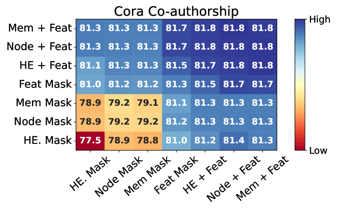
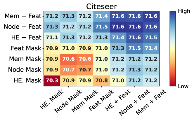
Figure 2: Node classification accuracy (%) when employing different augmentation pairs. Using the structural and attribute augmentations together always yields better performance than using just one.

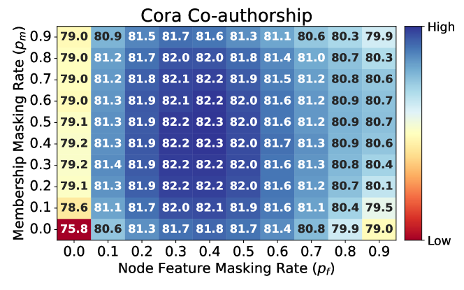
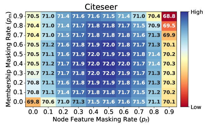
Figure 3: Node classification accuracy (%) according to the masking rates of membership and node features. A moderate extent of augmentation (i.e., masking rate between 0.3 and 0.7) benefits the downstream performance most.

Appendix E Additional Experiments

E.1 Ablation Study: Effects of Self-loops

In TriCL, we add self-loops to the hypergraph after hypergraph augmentation and before it is passed through the encoder. We conduct an ablation study to demonstrate the effects of self-loops. The results are summarized in Table 8, and it empirically verifies that adding self-loops is advantageous. The reason for the better performance we speculate is that a self-loop helps each node make a better use of its initial features. Specifically, a hyperedge corresponding to a self-loop receives a message only from the node it contains and sends a message back to the node without aggregating the features of any other nodes. This allows each node to make a better use of its features.

Table 8: Node classification accuracy (%) of TriCL when the hypergraphs, which the encoder receives as input, are with and without self-loops. Adding self-loops helps to improve the quality of the node representations.

Dataset	TriCL
	Without Self-loops	With Self-loops (Proposed)
Cora-C	80.95 $\pm$ 1.29	81.57 $\pm$ 1.12
Citeseer	71.10 $\pm$ 1.09	72.02 $\pm$ 1.16
Pubmed	84.02 $\pm$ 0.56	84.26 $\pm$ 0.62
Cora-A	79.77 $\pm$ 0.95	82.15 $\pm$ 0.89
DBLP	90.19 $\pm$ 0.12	91.12 $\pm$ 0.11
Zoo	80.43 $\pm$ 11.3	80.25 $\pm$ 11.2
20News	79.56 $\pm$ 0.24	80.14 $\pm$ 0.19
Mushroom	99.80 $\pm$ 0.14	99.83 $\pm$ 0.13
NTU2012	74.01 $\pm$ 2.54	75.23 $\pm$ 2.45
ModelNet40	93.48 $\pm$ 0.16	97.08 $\pm$ 0.13

E.2 Ablation Study: Backbone Encoder

The superiority of the encoder used in TriCL over HGNN is verified in Table 9. We compare the accuracy of two TriCL models that use (1) HGNN and (2) the mean pooling layer (proposed), respectively, as an encoder. TriCL with the mean pooling layer consistently and slightly outperforms the one with HGNN as an encoder. This result justifies our choice of using the mean pooling layer as our backbone encoder.

E.3 Sensitivity Analysis

We investigate the impact of hyperparameters used in TriCL, especially, $\tau_{g}$ and $\tau_{m}$ in Eq. (6) and (7) as well as $\omega_{g}$ and $\omega_{m}$ in Eq. (8), with the Citeseer and Cora Co-citation datasets. We only change these hyperparameters in this analysis, and the others are fixed as provided in Appendix C.2.

We conduct node classification while varying the values of $\tau_{g}$ and $\tau_{m}$ from 0.1 to 1.0 and report the accuracy gain over TriCL-N, which only considers node-level contrast, in Figure 4. From the figure, it can be observed that TriCL achieves an accuracy gain in most cases when both the temperature parameters are not too small (i.e., 0.1), as shown in the blue area in the figure. It indicates that pursuing excessive uniformity in the embedding space rather degrades the node classification performance (Wang and Liu 2021). We also conduct the same task while varying the values of $\omega_{g}$ and $\omega_{m}$ from $2^{-4}$ to $2^{4}$ and report the accuracy gain over TriCL-N, in Figure 5. Using a large $\omega_{g}$ and a small $\omega_{m}$ together degrades the performance. This causes model collapse by making the proportion of membership contrastive loss relatively larger than node and group contrastive losses.

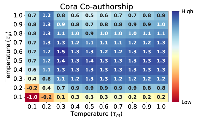
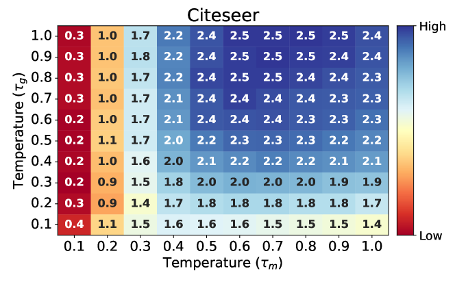
Figure 4: Node classification accuracy gain (%) of TriCL over TriCL-N, when different temperature parameter pairs are used. The baseline accuracies are 70.28% and 80.49% for the Citeseer and Cora Co-citation datasets, respectively.

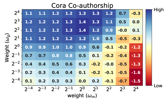
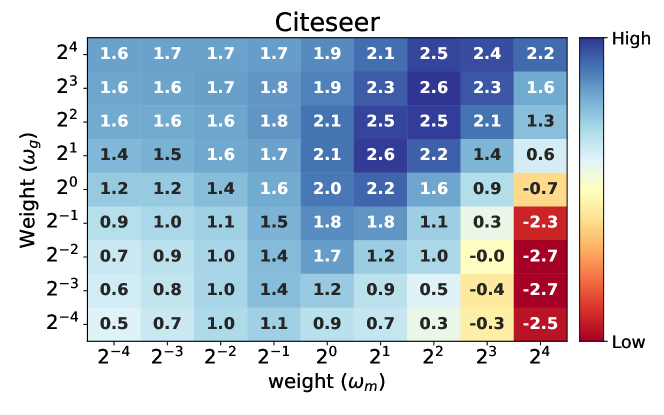
Figure 5: Node classification accuracy gain (%) of TriCL over TriCL-N, when different weight pairs are used. The baseline accuracies are 70.28% and 80.49% for the Citeseer and Cora Co-citation datasets, respectively.

Table 9: The accuracy of two TriCL methods that use (1) HGNN and (2) the mean pooling layer (proposed), respectively, as an encoder.

Dataset	TriCL (with HGNN)	TriCL (Proposed)
Cora-C	81.03 $\pm$ 1.31	81.57 $\pm$ 1.12
Citeseer	71.97 $\pm$ 1.26	72.02 $\pm$ 1.16
Pubmed	83.80 $\pm$ 0.63	84.26 $\pm$ 0.62
Cora-A	82.22 $\pm$ 1.09	82.15 $\pm$ 0.89
DBLP	90.93 $\pm$ 0.16	91.12 $\pm$ 0.11
Zoo	79.47 $\pm$ 11.0	80.25 $\pm$ 11.2
20News	79.93 $\pm$ 0.24	80.14 $\pm$ 0.19
Mushroom	98.93 $\pm$ 0.33	99.83 $\pm$ 0.13
NTU2012	74.63 $\pm$ 2.53	75.23 $\pm$ 2.45
ModelNet40	97.33 $\pm$ 0.14	97.08 $\pm$ 0.13

E.4 Training Time Comparison

We compare the training time of baseline models and TriCL by the elapsed time of a single epoch. We run each method for 50 epochs and measured the average elapsed time per epoch (ms). Note that subsampling is not used and TriCL computes the membership contrastive loss with mini-batches of size 4096 when training for the Pubmed, DBLP, 20News, Mushroom, and ModelNet40 datasets due to the memory limits. Generally, TriCL-NG shows similar execution times to baseline approaches, and TriCL is slower due to membership contrast.

Table 10: Single epoch running time (in milliseconds) averaged over 50 training epochs. The hyphen(-) indicates that the running time cannot be measured due to out of memory.

	Cora-C	Citeseer	Pubmed	Cora-A	DBLP	Zoo	20News	Mushroom	NTU2012	ModelNet40
DGI	4	4	16	4	76	4	-	-	4	13
GRACE	15	15	32	16	-	16	-	-	18	93
S2-HHGR	25	25	54	36	524	9	185	94	33	142
TriCL-N	13	12	18	11	488	10	78	37	11	50
TriCL-NG	19	17	38	17	625	15	83	40	16	85
TriCL	102	79	652	121	3,156	32	396	702	194	636

Appendix F Qualitative Analysis

F.1 Analysis on the Pubmed, Cora Co-authorship, and DBLP datasets

As additional experiments, in Table 11, We provide t-SNE (Van der Maaten and Hinton 2008) plots of the node representations produced by TriCL and its two variants, TriCL-N and TriCL-NG, on the Pubmed, Cora Co-authorship, and DBLP datasets. As expected from the quantitative results, the 2-D projection of embeddings learned by TriCL shows more numerically (based on Silhouette score (Rousseeuw 1987)) distinguishable clusters than its two variants.

Table 11: t-SNE plots of the node representations from TriCL and its two variants. The TriCL’s embeddings exhibits the most distinct clusters with the help of group and membership contrast, as measured by the Silhouette score (the higher, the better).

	Pubmed	Cora Co-authorship	DBLP
TriCL-N
TriCL-NG
TriCL

F.2 Analysis on the Collapsed Models

Using membership contrast alone sometimes causes model collapse. t-SNE plots of the collapsed models are shown in Figure 6. There is no clear distinction between the representations of nodes of different classes, and they overlap. It even looks randomly scattered around two clusters in the Citeseer dataset. One potential reason the model fails to produce separable embeddings is that there is no guidance between node representations or between edge representations. Using node or group contrast together, this problem could be solved.

(a) Citeseer

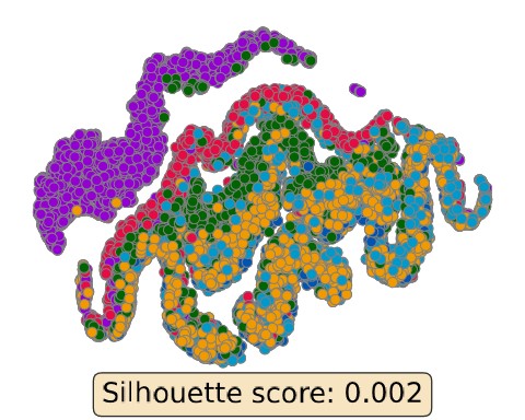
(b) DBLP

Figure 6: t-SNE plots of the node representations from TriCL when model collapse occurred. There is no clear distinction between the representations of nodes of different classes.

References

- Arthur and Vassilvitskii (2006) Arthur, D.; and Vassilvitskii, S. 2006. k-means++: The advantages of careful seeding. Technical report, Stanford.
- Arya et al. (2020) Arya, D.; Gupta, D. K.; Rudinac, S.; and Worring, M. 2020. Hypersage: Generalizing inductive representation learning on hypergraphs. arXiv:2010.04558.
- Bai, Zhang, and Torr (2021) Bai, S.; Zhang, F.; and Torr, P. H. 2021. Hypergraph convolution and hypergraph attention. Pattern Recognition, 110: 107637.
- Benson et al. (2018) Benson, A. R.; Abebe, R.; Schaub, M. T.; Jadbabaie, A.; and Kleinberg, J. 2018. Simplicial closure and higher-order link prediction. PNAS, 115(48).
- Benson, Gleich, and Leskovec (2016) Benson, A. R.; Gleich, D. F.; and Leskovec, J. 2016. Higher-order organization of complex networks. Science, 353(6295): 163–166.
- Chen et al. (2003) Chen, D.-Y.; Tian, X.-P.; Shen, Y.-T.; and Ouhyoung, M. 2003. On visual similarity based 3D model retrieval. Computer graphics forum, 22(3): 223–232.
- Chen et al. (2020) Chen, T.; Kornblith, S.; Norouzi, M.; and Hinton, G. 2020. A simple framework for contrastive learning of visual representations. In ICML, 1597–1607.
- Chien et al. (2022) Chien, E.; Pan, C.; Peng, J.; and Milenkovic, O. 2022. You are AllSet: A Multiset Function Framework for Hypergraph Neural Networks. In ICLR.
- Clevert, Unterthiner, and Hochreiter (2016) Clevert, D.-A.; Unterthiner, T.; and Hochreiter, S. 2016. Fast and accurate deep network learning by exponential linear units (elus). In ICLR.
- Do et al. (2020) Do, M. T.; Yoon, S.-e.; Hooi, B.; and Shin, K. 2020. Structural patterns and generative models of real-world hypergraphs. In KDD, 176–186.
- Dong, Sawin, and Bengio (2020) Dong, Y.; Sawin, W.; and Bengio, Y. 2020. HNHN: Hypergraph networks with hyperedge neurons. In ICML Workshop on Graph Representation Learning and Beyond.
- Dua and Graff (2017) Dua, D.; and Graff, C. 2017. UCI Machine Learning Repository.
- Feng et al. (2019) Feng, Y.; You, H.; Zhang, Z.; Ji, R.; and Gao, Y. 2019. Hypergraph neural networks. In AAAI, volume 33, 3558–3565.
- Feng et al. (2018) Feng, Y.; Zhang, Z.; Zhao, X.; Ji, R.; and Gao, Y. 2018. Gvcnn: Group-view convolutional neural networks for 3d shape recognition. In CVPR, 264–272.
- Fey and Lenssen (2019) Fey, M.; and Lenssen, J. E. 2019. Fast graph representation learning with PyTorch Geometric. arXiv:1903.02428.
- Gao, Yao, and Chen (2021) Gao, T.; Yao, X.; and Chen, D. 2021. Simcse: Simple contrastive learning of sentence embeddings. In EMNLP.
- Glorot and Bengio (2010) Glorot, X.; and Bengio, Y. 2010. Understanding the difficulty of training deep feedforward neural networks. In AISTATS, 249–256.
- Grover and Leskovec (2016) Grover, A.; and Leskovec, J. 2016. node2vec: Scalable feature learning for networks. In KDD, 855–864.
- Hassani and Khasahmadi (2020) Hassani, K.; and Khasahmadi, A. H. 2020. Contrastive multi-view representation learning on graphs. In ICML, 4116–4126.
- He et al. (2020) He, K.; Fan, H.; Wu, Y.; Xie, S.; and Girshick, R. 2020. Momentum contrast for unsupervised visual representation learning. In CVPR, 9729–9738.
- He et al. (2015) He, K.; Zhang, X.; Ren, S.; and Sun, J. 2015. Delving deep into rectifiers: Surpassing human-level performance on imagenet classification. In ICCV, 1026–1034.
- Hein et al. (2013) Hein, M.; Setzer, S.; Jost, L.; and Rangapuram, S. S. 2013. The total variation on hypergraphs-learning on hypergraphs revisited. In NIPS.
- Hjelm et al. (2019) Hjelm, R. D.; Fedorov, A.; Lavoie-Marchildon, S.; Grewal, K.; Bachman, P.; Trischler, A.; and Bengio, Y. 2019. Learning deep representations by mutual information estimation and maximization. In ICLR.
- Huang and Yang (2021) Huang, J.; and Yang, J. 2021. Unignn: a unified framework for graph and hypergraph neural networks. In IJCAI.
- Jaiswal et al. (2020) Jaiswal, A.; Babu, A. R.; Zadeh, M. Z.; Banerjee, D.; and Makedon, F. 2020. A survey on contrastive self-supervised learning. Technologies, 9(1): 2.
- Kingma and Ba (2015) Kingma, D. P.; and Ba, J. 2015. Adam: A method for stochastic optimization. In ICLR.
- Kipf and Welling (2017) Kipf, T. N.; and Welling, M. 2017. Semi-supervised classification with graph convolutional networks. In ICLR.
- Lee, Choe, and Shin (2022) Lee, G.; Choe, M.; and Shin, K. 2022. HashNWalk: Hash and Random Walk Based Anomaly Detection in Hyperedge Streams. In IJCAI.
- Lee, Ko, and Shin (2020) Lee, G.; Ko, J.; and Shin, K. 2020. Hypergraph motifs: concepts, algorithms, and discoveries. In Proceedings of the VLDB Endowment.
- Lee et al. (2019) Lee, J.; Lee, Y.; Kim, J.; Kosiorek, A.; Choi, S.; and Teh, Y. W. 2019. Set transformer: A framework for attention-based permutation-invariant neural networks. In ICML, 3744–3753.
- Li, Jing, and Tong (2022) Li, B.; Jing, B.; and Tong, H. 2022. Graph Communal Contrastive Learning. In WWW, 1203–1213.
- Li and Milenkovic (2018) Li, P.; and Milenkovic, O. 2018. Submodular hypergraphs: p-laplacians, cheeger inequalities and spectral clustering. In ICML, 3014–3023.
- Liu et al. (2021) Liu, X.; Zhang, F.; Hou, Z.; Mian, L.; Wang, Z.; Zhang, J.; and Tang, J. 2021. Self-supervised learning: Generative or contrastive. TKDE.
- Liu et al. (2022) Liu, Y.; Jin, M.; Pan, S.; Zhou, C.; Zheng, Y.; Xia, F.; and Yu, P. 2022. Graph self-supervised learning: A survey. TKDE.
- Lloyd (1982) Lloyd, S. 1982. Least squares quantization in PCM. IEEE Transactions on Information Theory, 28(2): 129–137.
- Loshchilov and Hutter (2019) Loshchilov, I.; and Hutter, F. 2019. Decoupled weight decay regularization. In ICLR.
- Oord, Li, and Vinyals (2018) Oord, A. v. d.; Li, Y.; and Vinyals, O. 2018. Representation learning with contrastive predictive coding. arXiv:1807.03748.
- Paszke et al. (2019) Paszke, A.; Gross, S.; Massa, F.; Lerer, A.; Bradbury, J.; Chanan, G.; Killeen, T.; Lin, Z.; Gimelshein, N.; Antiga, L.; et al. 2019. Pytorch: An imperative style, high-performance deep learning library. In NeurIPS.
- Peng et al. (2020) Peng, Z.; Huang, W.; Luo, M.; Zheng, Q.; Rong, Y.; Xu, T.; and Huang, J. 2020. Graph representation learning via graphical mutual information maximization. In WWW, 259–270.
- Qiu et al. (2020) Qiu, J.; Chen, Q.; Dong, Y.; Zhang, J.; Yang, H.; Ding, M.; Wang, K.; and Tang, J. 2020. Gcc: Graph contrastive coding for graph neural network pre-training. In KDD, 1150–1160.
- Rong et al. (2020) Rong, Y.; Huang, W.; Xu, T.; and Huang, J. 2020. Dropedge: Towards deep graph convolutional networks on node classification. In ICLR.
- Rossi and Ahmed (2015) Rossi, R.; and Ahmed, N. 2015. The network data repository with interactive graph analytics and visualization. In AAAI.
- Rousseeuw (1987) Rousseeuw, P. J. 1987. Silhouettes: a graphical aid to the interpretation and validation of cluster analysis. Journal of Computational and Applied Mathematics, 20: 53–65.
- Sen et al. (2008) Sen, P.; Namata, G.; Bilgic, M.; Getoor, L.; Galligher, B.; and Eliassi-Rad, T. 2008. Collective classification in network data. AI magazine, 29(3): 93–93.
- Su et al. (2015) Su, H.; Maji, S.; Kalogerakis, E.; and Learned-Miller, E. 2015. Multi-view convolutional neural networks for 3d shape recognition. In ICCV, 945–953.
- Thakoor et al. (2022) Thakoor, S.; Tallec, C.; Azar, M. G.; Azabou, M.; Dyer, E. L.; Munos, R.; Veličković, P.; and Valko, M. 2022. Large-scale representation learning on graphs via bootstrapping. In ICLR.
- Tschannen et al. (2019) Tschannen, M.; Djolonga, J.; Rubenstein, P. K.; Gelly, S.; and Lucic, M. 2019. On Mutual Information Maximization for Representation Learning. In ICLR.
- Van der Maaten and Hinton (2008) Van der Maaten, L.; and Hinton, G. 2008. Visualizing data using t-SNE. Journal of Machine Learning Research, 9(11).
- Veldt, Benson, and Kleinberg (2021) Veldt, N.; Benson, A. R.; and Kleinberg, J. 2021. Higher-order homophily is combinatorially impossible. arXiv:2103.11818.
- Veličković et al. (2018a) Veličković, P.; Cucurull, G.; Casanova, A.; Romero, A.; Liò, P.; and Bengio, Y. 2018a. Graph Attention Networks. In ICLR.
- Veličković et al. (2018b) Veličković, P.; Fedus, W.; Hamilton, W. L.; Liò, P.; Bengio, Y.; and Hjelm, R. D. 2018b. Deep Graph Infomax. In ICLR.
- Wang and Liu (2021) Wang, F.; and Liu, H. 2021. Understanding the behaviour of contrastive loss. In CVPR, 2495–2504.
- Wu et al. (2015) Wu, Z.; Song, S.; Khosla, A.; Yu, F.; Zhang, L.; Tang, X.; and Xiao, J. 2015. 3d shapenets: A deep representation for volumetric shapes. In CVPR, 1912–1920.
- Xia et al. (2021) Xia, X.; Yin, H.; Yu, J.; Wang, Q.; Cui, L.; and Zhang, X. 2021. Self-supervised hypergraph convolutional networks for session-based recommendation. In AAAI, volume 35, 4503–4511.
- Yadati et al. (2019) Yadati, N.; Nimishakavi, M.; Yadav, P.; Nitin, V.; Louis, A.; and Talukdar, P. 2019. Hypergcn: A new method for training graph convolutional networks on hypergraphs. In NeurIPS.
- Yang et al. (2019) Yang, D.; Qu, B.; Yang, J.; and Cudre-Mauroux, P. 2019. Revisiting user mobility and social relationships in lbsns: a hypergraph embedding approach. In WWW, 2147–2157.
- You et al. (2020) You, Y.; Chen, T.; Sui, Y.; Chen, T.; Wang, Z.; and Shen, Y. 2020. Graph contrastive learning with augmentations. In NeurIPS.
- Yu et al. (2021) Yu, J.; Yin, H.; Li, J.; Wang, Q.; Hung, N. Q. V.; and Zhang, X. 2021. Self-supervised multi-channel hypergraph convolutional network for social recommendation. In WWW, 413–424.
- Zaheer et al. (2017) Zaheer, M.; Kottur, S.; Ravanbakhsh, S.; Poczos, B.; Salakhutdinov, R. R.; and Smola, A. J. 2017. Deep sets. In NIPS.
- Zhang et al. (2021) Zhang, J.; Gao, M.; Yu, J.; Guo, L.; Li, J.; and Yin, H. 2021. Double-Scale Self-Supervised Hypergraph Learning for Group Recommendation. In CIKM, 2557–2567.
- Zhang et al. (2022) Zhang, J.; Li, F.; Xiao, X.; Xu, T.; Rong, Y.; Huang, J.; and Bian, Y. 2022. Hypergraph Convolutional Networks via Equivalency between Hypergraphs and Undirected Graphs. arXiv:2203.16939.
- Zheng et al. (2019) Zheng, X.; Zhu, W.; Tang, C.; and Wang, M. 2019. Gene selection for microarray data classification via adaptive hypergraph embedded dictionary learning. Gene, 706: 188–200.
- Zhou, Huang, and Schölkopf (2006) Zhou, D.; Huang, J.; and Schölkopf, B. 2006. Learning with hypergraphs: Clustering, classification, and embedding. In NIPS.
- Zhu et al. (2021a) Zhu, R.; Zhao, B.; Liu, J.; Sun, Z.; and Chen, C. W. 2021a. Improving contrastive learning by visualizing feature transformation. In ICCV, 10306–10315.
- Zhu et al. (2020) Zhu, Y.; Xu, Y.; Yu, F.; Liu, Q.; Wu, S.; and Wang, L. 2020. Deep graph contrastive representation learning. In ICML Workshop on Graph Representation Learning and Beyond.
- Zhu et al. (2021b) Zhu, Y.; Xu, Y.; Yu, F.; Liu, Q.; Wu, S.; and Wang, L. 2021b. Graph contrastive learning with adaptive augmentation. In WWW, 2069–2080.