EMPRESS. IX.
Extremely Metal-Poor Galaxies are Very Gas-Rich Dispersion-Dominated Systems:
Will JWST Witness Gaseous Turbulent High-$z$ Primordial Galaxies?

Abstract

We present kinematics of 6 local extremely metal-poor galaxies (EMPGs) with low metallicities ($0.016-0.098\ Z_{\odot}$) and low stellar masses ($10^{4.7}-10^{7.6}M_{\odot}$). Taking deep medium-high resolution ($R\sim 7500$) integral-field spectra with 8.2-m Subaru, we resolve the small inner velocity gradients and dispersions of the EMPGs with H$\alpha$ emission. Carefully masking out sub-structures originated by inflow and/or outflow, we fit 3-dimensional disk models to the observed H$\alpha$ flux, velocity, and velocity-dispersion maps. All the EMPGs show rotational velocities ($v_{\rm rot}$) of 5–23 km s^-1 smaller than the velocity dispersions ($\sigma_{0}$) of 17–31 km s^-1, indicating dispersion-dominated ($v_{\rm rot}/\sigma_{0}=0.29-0.80<1$) systems affected by inflow and/or outflow. Except for two EMPGs with large uncertainties, we find that the EMPGs have very large gas-mass fractions of $f_{\rm gas}\simeq 0.9-1.0$. Comparing our results with other H$\alpha$ kinematics studies, we find that $v_{\rm rot}/\sigma_{0}$ decreases and $f_{\rm gas}$ increases with decreasing metallicity, decreasing stellar mass, and increasing specific star-formation rate. We also find that simulated high-$z$ ($z\sim 7$) forming galaxies have gas fractions and dynamics similar to the observed EMPGs. Our EMPG observations and the simulations suggest that primordial galaxies are gas-rich dispersion-dominated systems, which would be identified by the forthcoming James Webb Space Telescope (JWST) observations at $z\sim 7$.

1 Introduction

Primordial galaxies characterized by low metallicities and low stellar masses are important to understand galaxy formation. Cosmological and hydrodynamical simulations (e.g., Wise et al., 2012; Yajima et al., 2022) have predicted that primordial galaxies at $z\sim 10$ would form in low-mass halos with halo masses of $\sim 10^{8}\ M_{\odot}$. Such simulated primordial galaxies at $z\gtrsim 7$ show low gas-phase metallicities of $\lesssim 1$% of the solar abundance ($Z_{\odot}$), specific star-formation rates (sSFRs) of $\sim 100$ Gyr^-1, and low stellar masses of $\lesssim 10^{6}\ M_{\odot}$. Despite their scientific relevance, it is difficult to observe primordial galaxies due to their faintness. Isobe et al. (2022; hereafter Paper IV) have estimated an H$\alpha$ flux of a primordial galaxy with $M_{*}=10^{6}\ M_{\odot}$ as a function of redshift, and demonstrated that even the current-best spectrographs such as Keck/LRIS or Keck/MOSFIRE cannot observe the primordial galaxy at $z\gtrsim 0.5$ without any gravitational lensing magnification (e.g., Kikuchihara et al., 2020).

Kinematics of high-$z$ primordial galaxies can provide us a hint of what kind of mechanism (e.g., inflow/outflow) would impact on the early galaxy formation. We are still lacking a good handle on the detailed gas dynamical state, often quantified in broad terms by the relative level of rotation, via the $v_{\rm rot}/\sigma_{0}$ ratio (e.g., Förster Schreiber et al., 2009). Integral-field unit (IFU) observations (e.g., Wisnioski et al., 2015; Herrera-Camus et al., 2022) have reported that star-forming galaxies show $v_{\rm rot}/\sigma_{0}$ ratios decreasing from $v_{\rm rot}/\sigma_{0}\sim 10$ to $\sim 2$ with increasing redshift from $z\sim 0$ to 5.5, while such observations are currently limited to massive ($\sim 10^{10}\ M_{\odot}$) galaxies. It is important to directly determine whether low-mass ($\lesssim 10^{6}\ M_{\odot}$) primordial galaxies are truly dominated by dispersion.

Complementary to the high-$z$ kinematics studies, some studies have reported $v_{\rm rot}/\sigma_{0}$ values of local galaxies with lower stellar masses. Local galaxies are advantageous for conducting deep observations with high spectral and spatial resolutions. The SH$\alpha$DE survey (Barat et al., 2020) has made a significant progress in extracting $v_{\rm rot}$ and $\sigma_{0}$ values of local dwarf galaxies with stellar masses down to $\sim 10^{6}\ M_{\odot}$. These observations suggest that the ratio $v_{\rm rot}/\sigma_{0}$ decreases down to $\lesssim 1$ with decreasing $M_{*}$ down to $\sim 10^{6}\ M_{\odot}$. However, the SH$\alpha$DE galaxies have gas-phase oxygen metallicities higher than $12+\log(\rm O/H)\sim 7.69$ that correspond to $Z\sim 0.1\ Z_{\odot}$ (Asplund et al., 2021), which are still $\gtrsim 1$ dex higher than that of the simulated high-$z$ primordial galaxy (Wise et al., 2012).

To understand the kinematic properties of chemically-primordial galaxies, we investigate H$\alpha$ kinematics of local galaxies with $Z\leq 0.1\ Z_{\odot}$ that are often referred to as extremely metal-poor galaxies (e.g., Kunth & Östlin, 2000; Izotov et al., 2012), abbreviated as EMPGs (Kojima et al. 2020, hereafter Paper I). Although EMPGs become rarer toward lower redshifts (Morales-Luis et al., 2011), various studies have reported the presence of EMPGs in the local universe. Representative and well-studied EMPGs are SBS0335$-$052 (Izotov et al., 2009), AGC198691 (Hirschauer et al., 2016), Little Cub (Hsyu et al., 2017), DDO68 (Pustilnik et al., 2005), IZw18 (Izotov & Thuan, 1998), and Leo P (Skillman et al., 2013). Izotov et al. (2018) have pinpointed J0811+4730 with a low metallicity of 0.02 $Z_{\odot}$.

Recently, a project “Extremely Metal-Poor Representatives Explored by the Subaru Survey (EMPRESS)” has been launched (Paper I). EMPRESS aims to select faint EMPG photometric candidates from Subaru/Hyper Suprime-Cam (HSC; Miyazaki et al. 2018) deep optical ($i_{\rm lim}=26$ mag; Aihara et al. 2019) images, which are $\sim 2$ dex deeper than those of SDSS. Conducting follow-up spectroscopic observations of the EMPG photometric candidates, EMPRESS has identified new 12 EMPGs with low stellar masses of $10^{4.2}$–$10^{6.6}\ M_{\odot}$ (Papers I, IV; Nakajima et al. 2022, hereafter Paper V; Xu et al. 2022, hereafter Paper VI). Remarkably, J1631+4426 has been reported to have a metallicity of 0.016 $Z_{\odot}$, which is the lowest metallicity idenitifed so far (Paper I).

Including the 12 low-mass EMPGs found by EMPRESS, Paper V summarizes 103 local EMPGs identified so far whose metallicities are accurately measured with the direct-temperature method (e.g., Izotov et al., 2006). The 103 EMPGs show low metallicities of 0.016–0.1 $Z_{\odot}$, low stellar masses of $\sim 10^{4}$–$10^{8}\ M_{\odot}$, and high sSFRs of $\sim 1$–$400$ Gyr^-1 (Paper V). These features resemble the simulated primordial galaxy at $z\gtrsim 7$ (Wise et al., 2012), suggesting that EMPGs would be good local analogs of high-$z$ primordial galaxies (but see also Isobe et al. 2021, hereafter Paper III).

This paper is the ninth paper of EMPRESS, reporting H$\alpha$ kinematics of EMPGs observed with Subaru/Faint Object Camera and Spectrograph (FOCAS) IFU (Ozaki et al., 2020) in a series of the Subaru Intensive Program entitled EMPRESS 3D (PI: M. Ouchi). So far, EMPRESS has released 8 papers related to EMPGs, each of which reports the survey design (Paper I), high Fe/O ratios suggestive of massive stars (Kojima et al. 2021, hereafter Paper II; Paper IV), morphology (Paper III), low-$Z$ ends of metallicity diagnostics (Paper V), outflows (Paper VI), the shape of incident spectrum that reproduces high-ionization lines (Umeda et al. 2022, hereafter Paper VII), and the primordial He abundance (Matsumoto et al. 2022, hereafter Paper VIII).

This paper is organized as follows. Section 2 explains our observational targets. The observations are summarized in Section 3. Section 4 reports H$\alpha$ flux, velocity, and velocity-dispersion maps of our targets. Our kinematic analysis is described in Section 5. Section 6 lists our results. We discuss kinematics of primordial galaxies in Section 7. Our findings are summarized in Section 8. Throughout this paper, magnitudes are in the AB system (Oke & Gunn, 1983). We assume a standard $\Lambda$CDM cosmology with parameters of ($\Omega_{\rm m}$, $\Omega_{\rm\Lambda}$, $H_{0}$) = (0.3, 0.7, 70 km ${\rm s}^{-1}$ ${\rm Mpc}^{-1}$). The solar metallicity $Z_{\odot}$ is defined by $12+\log(\rm O/H)=8.69$ (Asplund et al., 2021).

2 Sample

Table 1: Properties of the observed 6 EMPGs

#	Name	R.A.	Decl.	Redshift	$12+\log(\rm O/H)$	$\log(M_{*})$	$\log(\rm SFR)$	$\log(\rm sSFR)$
		hh:mm:ss	dd:mm:ss			$M_{\odot}$	$M_{\odot}$ yr-1	Gyr-1
(1)	(2)	(3)	(4)	(5)	(6)	(7)	(8)	(9)
1	J1631+4426	16:31:14.24	+44:26:04.43	0.0313	$6.90\pm 0.03^{{\color[rgb]{0,0,1}1}}$	$5.9^{{\color[rgb]{0,0,1}1}}$	$-1.3^{{\color[rgb]{0,0,1}1}}$	1.8
2	IZw18NW	09:34:02.03	+55:14:28.07	0.0024	$7.16\pm 0.01^{{\color[rgb]{0,0,1}2}}$	$7.1^{{\color[rgb]{0,0,1}3}}$	$-1.4^{{\color[rgb]{0,0,1}4}}$	0.5
3	SBS0335$-$052E	03:37:44.06	$-$05:02:40.19	0.0135	$7.22\pm 0.07^{{\color[rgb]{0,0,1}5}}$	$7.6^{{\color[rgb]{0,0,1}5}}$	$-0.4^{{\color[rgb]{0,0,1}4}}$	1.0
4	HS0822+3542	08:25:55.44	+35:32:31.92	0.0020	$7.45\pm 0.02^{{\color[rgb]{0,0,1}6}}$	4.67	$-2.2^{{\color[rgb]{0,0,1}8}}$	2.2
5	J1044+0353	10:44:57.79	+03:53:13.15	0.0130	$7.48\pm 0.01^{{\color[rgb]{0,0,1}6}}$	6.07	$-0.9^{{\color[rgb]{0,0,1}9}}$	2.1
6	J2115$-$1734	21:15:58.33	$-$17:34:45.09	0.0230	$7.68\pm 0.01^{{\color[rgb]{0,0,1}1}}$	$6.6^{{\color[rgb]{0,0,1}1}}$	$0.3^{{\color[rgb]{0,0,1}1}}$	2.7

We select 6 EMPGs visible on the observing nights (Section 3.1) and having relatively strong H$\beta$ fluxes at a given metallicity so that we obtain kinematics of the EMPGs with high signal-to-noise (SN) ratios. Details of the observational strategy will be reported in Xu et al. (in prep.). The 6 EMPGs consists of J1631+4426 (Paper I), IZw18 (e.g., Searle & Sargent, 1972), SBS0335$-$052E (e.g., Izotov et al., 1997), HS0822+3542 (Kniazev et al., 2000), J1044+0353 (Papaderos et al., 2008), and J2115$-$1734 (Paper I).

We note that the 4 EMPGs other than J1631+4426 or J2115$-$1734 have radio and/or optical integral-field spectroscopy conducted by previous studies. IZw18 has H i observations with VLA (Lelli et al., 2012). SBS0335$-$052E also has VLA H i observations (Pustilnik et al., 2001) as well as VLT/MUSE H$\alpha$ observations with a spectral resolution of $R\sim 3000$ (Herenz et al., 2017). Our observations with FOCAS IFU are complementary to those previous observations of IZw18 and SBS0335$-$052E because of our higher spectral resolution ($R\sim 7500$, Section 3.1). HS0822+3542 and J1044+0353 have H$\alpha$ observations with 6-m BTA/Fabry-Perot interferometer having $R\sim 8000$ (Moiseev et al., 2010). FOCAS IFU can detect emission lines $\sim 2$ times fainter than those of Fabry-Perot interferometer with a similar spectral resolution.

Properties of the observed 6 EMPGs are listed in Table 1. The 6 EMPGs have low metallicities of $12+\log(\rm O/H)=6.90$–7.68, low stellar masses of $\log(M_{*}/M_{\odot})=4.7$–7.6, and high specific star-formation rates of $\log(\rm sSFR/Gyr^{-1})=0.5$–2.7. These properties indicate that the 6 EMPGs are the best available analogs of primordial galaxies in the early universe. We emphasize that the 6 EMPGs include J1631+4426 having $12+\log(\rm O/H)=6.90$ (Paper I), which is the lowest gas-phase metallicity among galaxies identified so far.

3 Observations and data analysis

3.1 Observations and Data Reduction

This section reports our spectroscopic observations with FOCAS IFU (Ozaki et al., 2020). FOCAS IFU is an IFU with an image slicer installed in FOCAS (Kashikawa et al., 2002) mounted on a Cassegrain focus of the Subaru 8.2-m telescope. The large diameter of the Subaru Telescope allows FOCAS IFU to perform deep integral-field spectroscopy with a 5$\sigma$ limiting flux of $\sim 1\times 10^{-17}$ erg s^-1 cm^-2 arcsec^-2 (Ozaki et al., 2020). The FoV of FOCAS IFU is $13.\!\!\arcsec 5$ (slice length direction; hereafter X direction) $\times$ $10.\!\!\arcsec 0$ (slice width direction; hereafter Y direction). The pixel scale in a reduced data cube is $0.\!\!\arcsec 215$ (X direction) and $0.\!\!\arcsec 435$ (Y direction).

We carried out spectroscopy with FOCAS IFU for the 6 EMPGs (Section 2). The observing nights were 2021 August 13, November 24, and December 13. We set pointing positions so that the whole structures of EMPGs are covered with single FoVs.

We used the mid-high-dispersion grism of VPH680 offering the spectral resolution of $R\sim 7500$. We took comparison frames of the ThAr lamp. We observed Feige67, HZ44, BD28, Feige110, and Feige34 as standard stars. All the nights were clear with seeing sizes of $\sim 0.\!\!\arcsec 7$.

We use a reduction pipeline software of FOCAS IFU based on PyRAF (Tody, 1986) and Astropy (Astropy Collaboration et al., 2013). The software performs bias subtraction, flat-fielding, cosmic-ray cleaning, sky subtraction, wavelength calibration with the comparison frames, and flux calibration. We estimate flux errors containing read-out noises and photon noises of sky and object emissions.

It should be noted that there remain systematic velocity differences among the slices even after the wavelength calibration with the comparison frames. We conducted additional wavelength calibration with sky emission lines around observed wavelengths of H$\alpha$.

3.2 Flux, Velocity, and Velocity Dispersion Measurement

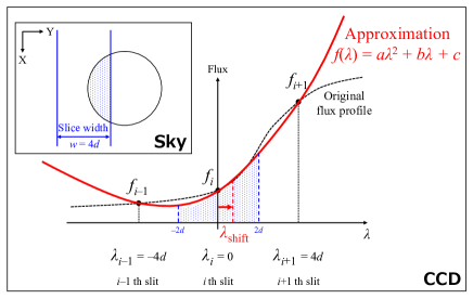
Figure 1: Explanation of the slit-width effect. The inset panel shows a schematic figure of an object on the celestial sphere. The X (Y) direction denotes the slice length (width) direction. The blue solid lines describe the position of the single slice. The light coming into the slice (blue shaded) is projected onto the CCD, where the Y direction in the sky is parallel to the wavelength ($\lambda$) direction on the CCD. The original spatial flux profile projected onto the CCD (black dashed curve) provides fluxes of ($i-1$), $i$, and ($i+1$)th slices ($f_{i-1},\ f_{i}$, and $f_{i+1}$, respectively). The original flux profile is assumed to be approximated by the quadratic function $f(\lambda)=a\lambda^{2}+b\lambda+c$ (red solid curve) within the $\lambda$ range from $-2d$ to $2d$. We estimate the systematic wavelength shift originating from the slit-width effect ($\lambda_{\rm shift}$) from a barycenter of the flux following $f(\lambda)$ intercepted by the slice.

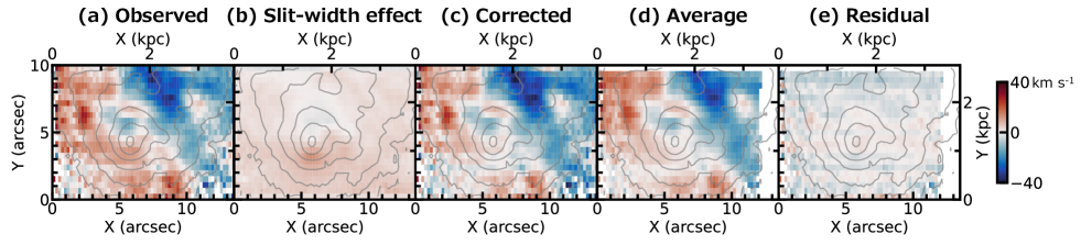
Figure 2: Confirmation of the slit-width effect correction using SBS0335$-$052E. (a) Observed velocity map. (b) Velocity shift generated by the slit-width effect. (c) Velocity map corrected for the slit-width effect. (d) Average of the 2 velocity maps whose position angles are different by 180 degree. (e) Residual of the corrected map and the average map. The gray contours illustrate SN ratios in the order of 5, 10, 20, … from the outside.

Figure 3: (Left) Residual of the observed velocity map and the average map in Figure 2. (Right) Residual of the corrected map and the average map, i.e., same as panel (e) in Figure 2, but with the smaller velocity range.

At all the spaxels, we fit H$\alpha$ lines using a single Gaussian function (+ constant) to measure H$\alpha$ fluxes, (relative) velocities, and velocity dispersions. We derive a line-spread function (LSF) by measuring widths of sky lines. A typical sky line has a full-width half maximum (FWHM) of $\sim 0.8$–1 Å. Assuming that both the H$\alpha$ lines from the EMPGs and the sky lines agree well with the Gaussian function, we obtain the intrinsic velocity dispersions by subtracting the LSFs from the observed velocity dispersions quadratically. We confirm that the assumption is reasonable for most of the H$\alpha$ lines and the sky lines other than some turbulent regions with multiple velocity components (Section 4).

We estimate the errors of the velocities and velocity dispersions by running the Monte Carlo simulations similar to the procedure of Herenz et al. (2016). We make 100 mock data cubes from our data cubes perturbed by the noise data cubes, and measure the velocities and velocity dispersions from each mock data cube. We regard the standard deviations of the derived velocities and velocity dispersions as the errors. The errors include the uncertainties of the LSFs, the additional wavelength calibration with the sky lines (Section 3.1), and the slit-width effect correction (see Section 3.3), because we perform these corrections using each mock data cube. Typical uncertainties of the velocity and velocity dispersion in each spaxel are $\sim 1.7$ and $\sim 1.6$ km s^-1, respectively. We self-consistently obtain the errors of the kinematic parameters in Sections 5.2 and 5.3 based on the 100 mock data cubes, in the same manner as we measure the errors of the velocities and velocity dispersions.

3.3 Slit-width Effect Correction

It should be noted that the observed velocities suffer from systematic wavelength shifts known as the slit-width effect (e.g., Bacon et al., 1995). Figure 1 illustrates the mechanism of the slit-width effect. The artificial wavelength shift is caused by a flux gradient in the Y direction (in each slice) that follows the dispersion (wavelength) axis ($\lambda$ direction thereafter) on the CCD.

Assuming a 2D Gaussian function for the (spatial) flux profile (i.e., assuming a point source), Bacon et al. (1995) have derived the wavelength shifts originating from the slit-width effect. Considering that all our targets are extended and complex sources, we expanded the method to more flexible flux profiles. The wavelength shift $\lambda_{\rm shift}$ can be estimated from a barycenter of the flux intercepted by the slice as follows:

$$\lambda_{\rm shift}=\frac{\int_{-0.5w}^{0.5w}\lambda f(\lambda){\rm d}\lambda}{\int_{-0.5w}^{0.5w}f(\lambda){\rm d}\lambda},$$ (1)

where $w$ and $f(\lambda)$ are a slice width projected onto the CCD and a flux profile in the Y direction, respectively. Because the pseudo slit width is sampled by 4 pixels for each slice, $w$ in the unit of Å is given by $w=4d$, where $d$ is a dispersion in the unit of Å pixel^-1.

We approximate $f(\lambda)$ by a quadratic function $f(\lambda)=a\lambda^{2}+b\lambda+c$ so that the function form is determined by the 3 points ($\lambda_{i-1}$, $f_{i-1}$), ($\lambda_{i}$, $f_{i}$), and ($\lambda_{i+1}$, $f_{i+1}$) in Figure 1, where $f_{i-1}$, $f_{i}$, and $f_{i+1}$ represent fluxes of $(i-1)$th, $i$th, and $(i+1)$th slices, respectively. In this case, $\lambda_{\rm shift}$ can be calculated as follows:

$$\lambda_{\rm shift} = \frac{\int_{-2d}^{2d}\lambda(a\lambda^{2}+b\lambda+c){\rm d}\lambda}{\int_{-2d}^{2d}(a\lambda^{2}+b\lambda+c){\rm d}\lambda}$$ (2)

$$= \frac{4bd^{2}}{4ad^{2}+3c}.$$

We derive $a$, $b$, and $c$ from the equations below:

$$a = \frac{f_{i-1}-2f_{i}+f_{i+1}}{16d^{2}}$$

$$b = \frac{f_{i+1}-f_{i-1}}{4d}$$ (3)

$$c = f_{i}.$$

Using Equations 2 and 3.3, we obtain

$$\lambda_{\rm shift}=\frac{4(f_{i+1}-f_{i-1})}{f_{i-1}+10f_{i}+f_{i+1}}d.$$ (4)

We infer from Equation 4 that high-dispersion dispersers make the slit-width effect weak. VPH680 has only $d=0.22$ Å pixel^-1, which results in velocity shifts produced by the slit-width effect of only $\sim\pm 10$ km s^-1 under the assumption of the seeing size of $0.\!\!\arcsec 7$. Although the velocity shift ($\sim 10$ km s^-1) is small, it is important to correct the slit-width effect because the low-mass EMPGs are expected to have small velocity gradients (Section 4).

Panel (a) of Figure 2 shows an observed velocity map of one of the EMPGs (SBS0335$-$052E), and panel (b) represents velocity shifts caused by the slit-width effect. A velocity map corrected for the slit-width effect is shown in panel (c).

To test our slit-width effect correction, we observed SBS0335$-$052E with 2 frames whose position angles are different by 180 degree. We expect that an average of the 2 velocity maps obtained from the 2 frames cancel out the slit-width effect. Panel (d) of Figure 2 shows the average map, and panel (e) represents residuals of the corrected map and the average map. The residuals are smaller than the velocity shifts caused by the slit-width effect. Figure 3 compares residuals of the observed velocity map and the average map (i.e., residuals NOT corrected for the slit-width effect; left) and residuals of the corrected velocity map and the average map (i.e., residuals corrected for the slit-width effect; right). Figure 3 shows that the residuals get much smaller after the slit-width effect correction. The small residuals of $\sim\pm 5$ km s^-1 also indicate that the corrected map agrees well with the average map. Thus, we conclude that our slit-width correction works well.

We evaluate the uncertainty of the slit-width effect correction by performing Monte Carlo simulation based on flux errors. A typical value of the uncertainty is 0.3 km s^-1.

4 Flux, Velocity, & Dispersion Maps

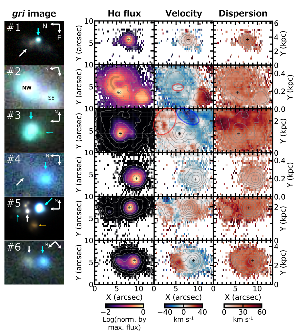
Figure 4: (Left) $gri$ images of the 6 EMPGs cut out of the FoV of FOCAS IFU. The numbers correspond to those in Table 1. The images of #1 and 5 are drawn from the HSC-SSP PDR3 (Aihara et al., 2022), while the others are taken from the Pan-STARRS catalog (Flewelling et al., 2020). (Middle left) Observed H$\alpha$ flux maps. The flux values in each flux map are normalized by the maximum flux value of each EMPG. The black crosses show flux peaks. The gray contours are the same as those in Figure 2. (Middle right) Velocity maps showing relative velocities that fit well in the velocity range from $-40$ to $40$ km s^-1. The velocity values are corrected for the slit-width effect (Section 3.3). (Right) Intrinsic velocity-dispersion maps (Section 3.3).

Figure 4 summarizes H$\alpha$ flux, velocity, and velocity dispersion maps of the 6 EMPGs as well as $gri$ images cut out of the FoV of FOCAS IFU. We note that only 2 EMPGs of #1 and 5 (i.e., J1631+4426 and J1044+0353) have images of the HSC-Subaru Strategic Program (SSP) Public Data Release (PDR) 3 (Aihara et al., 2022). The deep HSC images of the 2 EMPGs are shown in Figure 4, while the other $gri$ images are taken from the Pan-STARRS catalog (Flewelling et al., 2020). We report morphological and kinematic features of each EMPG below, checking the consistency with previous IFU studies.

#1 J1631+4426: The HSC $gri$ image illustrates that J1631+4426 consists of a blue clump (indicated by the cyan arrow) and a white diffuse structure elongated from north to south (white arrow). We refer to the white structure as the “EMPG tail” (Paper III). The H$\alpha$ flux map shows that the H$\alpha$ flux of J1631+4426 is dominated by the blue clump, which indicates that star formation in J1631+4426 should mainly occur in that region. Paper I has confirmed that the blue clump has the very low metallicity of $12+\log(\rm O/H)=6.90$ (Section 2) based on the direct-temperature method, while the EMPG tail can have a metallicity even lower than the blue clump based on the [O iii]$\lambda$5007/H$\alpha$ ratio (Kashiwagi et al., 2021). The velocity map shows that the blue clump is discontinuously redshifted by $\sim 20$ km s^-1 with respect to the EMPG tail, which indicates that the blue clump and the EMPG tail are not in the same kinematic structure. The blue clump itself shows a weak velocity gradient of $\sim 10$ km s^-1 from east to west, while the velocity dispersion is relatively high ($\sim 25$ km s^-1).

#2 IZw18: IZw18 has 2 main blue clumps of IZw18 Northwest (NW) and IZw18 Southeast (SE), both of which have been confirmed to be EMPGs (Izotov & Thuan, 1998). IZw18NW is blueshifted by $\sim 40$ km s^-1 with respect to IZw18SE (at around their flux peaks), consistent with the H i gas kinematics (Lelli et al., 2012). We thus think that IZw18NW and IZw18SE are not in the same kinematic structure. IZw18NW shows a complex morphokinematic structure. In the H$\alpha$ flux map, we find that the arc-like structure indicated by the gray curve (H$\alpha$ arc; Dufour & Hester 1990) has a velocity similar to that of IZw18NW, which indicates that the H$\alpha$ arc and IZw18NW belong to the same kinematic structure. In the velocity map, we also identify a velocity structure that is redshifted by $\sim 20$ km s^-1 with respect to the flux peak of IZw18NW (red circle). The velocity structure has a relatively high velocity dispersion of $\sim 30$ km s^-1, which implies that the structure is not settled. IZw18NW itself does not show a clear bulk rotation (i.e., not likely to be dominated by rotation).

#3 SBS0335$-$052E: The $gri$ image shows that SBS0335$-$052E consists of a large blue clump (thick cyan arrow) and a western subclump (thin cyan arrow). In the velocity map, we confirm that SBS0335$-$052E has a redshifted ($\sim+20$ km s^-1) region at northeast (red circle) and a blueshifted ($\sim-30$ km s^-1) region at northwest (blue circle). The redshifted and blueshifted regions seem connected to the northeast and north filaments identified with the wide-field MUSE H$\alpha$ observations (Herenz et al., 2017), respectively. Both regions have relatively high velocity dispersions of $\sim 60$ km s^-1, which agree with the scenario that the 2 structures are created by outflows (Herenz et al., 2017). The southern area of SBS0335$-$052E generally shows a relatively low velocity dispersion of $\sim 30$ km s^-1, which indicates that the southern area is relatively settled. The southern area shows a bulk velocity gradient of $\sim 20$ km s^-1 from northwest to southeast.

#4 HS0822+3542: HS0822+3542 consists of a blue clump (cyan arrow) and a very diffuse EMPG tail elongated from southeast to northwest (white arrow). The H$\alpha$ map indicates that the major star formation occurs in the blue clump. We find a very weak velocity gradient of $\sim 5$ km s^-1 in the blue clump from north to south. HS0822+3542 shows a high velocity dispersion of $\sim 20$ km s^-1, which is comparable to the previous observations (Moiseev et al., 2010).

#5 J1044+0353: The deep HSC image shows that J1044+0353 is composed of a western giant blue clump (thick cyan arrow), an eastern small blue clump (thin cyan arrow), and 3 white clumps between the 2 blue clumps (white arrow). We regard the 3 white clumps as the EMPG tail. The H$\alpha$ map indicates that the major star formation occurs in the giant blue clump. We obtain similar velocity and velocity dispersion maps to Moiseev et al. (2010)’s result, while we show more clearly that the small blue clump emits H$\alpha$. We find that the 2 blue clumps are redshifted by $\sim 20$ km s^-1 with respect to the EMPG tail, which indicate that the 2 blue clumps and the EMPG tail are not in the same kinematic structure. We find that the giant blue clump has a weak velocity gradient of $\sim 20$ km s^-1 from southeast to northwest, while the velocity dispersion ($\sim 30$ km s^-1) is quite high.

#6 J2115$-$1734: J2115$-$1734 consists of a blue clump (cyan arrow) and a north-east EMPG tail (white arrow). The majority of star formation is likely to occur in the blue clump. The EMPG tail is redshifted by $\sim 40$ km s^-1 with respect to the blue clump. Although the observed velocity field continuously changes between the blue clump and the EMPG tail, J2115$-$1734 shows a relatively high velocity dispersion of $\sim 40$ km s^-1 originating from 2 different velocity components. The blue clump itself has a weak velocity gradient of $\sim 20$ km s^-1 from northeast to southwest with a velocity dispersion of $\sim 30$ km s^-1.

In summary, all 6 EMPGs look irregular and dominated by dispersion rather than rotation. Their rotation velocities are not likely to be significant. In Section 5, we analyze the kinematics of the EMPGs more quantitatively.

5 Kinematic Analysis

5.1 Masking

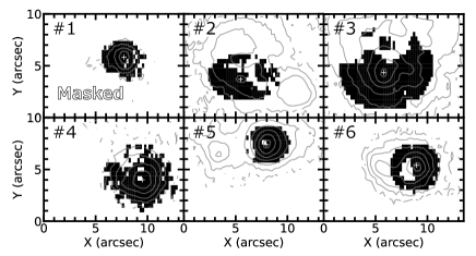
Figure 5: Mask map. The white regions correspond to the masked regions (Section 5.1).

Below, we quantify the level of rotation of the EMPGs by assuming that those systems are represented by a single rotating disk. The dynamical center of the disk is thought to be located at the H$\alpha$ flux peak of the main blue clump (IZw18NW for IZw18) under the assumptions of the gas-mass dominance on the galactic scale (cf. e.g., Herrera-Camus et al., 2022) and the empirical positive correlation between the gas mass surface density $\Sigma_{\rm gas}$ and the SFR surface density $\Sigma_{\rm SFR}$ (a.k.a. Kennicutt-Schmidt law; Kennicutt 1998). We confirm that these assumptions are reasonable by deriving the mass profile of each EMPG (Section 6.2). In the following analysis, we use only the region within the Kron radius of the main blue clump to remove the contamination from EMPG tails (IZw18SE for IZw18). We also mask spaxels with velocity dispersions higher than the flux-weighted 84th percentile of the distribution of the velocity dispersions because such regions are thought to be highly turbulent (Egorov et al., 2021). The white regions of Figure 5 show the masked regions.

5.2 Non-parametric Method

Table 2: Kinematic properties of the 6 EMPGs

#	Name	$v_{\rm shear}$	$\sigma_{\rm med}$	$v_{\rm shear}/\sigma_{\rm med}$	$v_{\rm rot}$	$\sigma_{0}$	$v_{\rm rot}/\sigma_{0}$
		km s-1	km s-1		km s-1	km s-1
(1)	(2)	(3)	(4)	(5)	(6)	(7)	(8)
1	J1631+4426	$10.3\pm 1.3$	$25.6\pm 0.4$	$0.40\pm 0.05$	$7.9\pm 1.8$	$25.6\pm 0.3$	$0.31\pm 0.08$
2	IZw18NW	$7.7\pm 0.4$	$23.2\pm 0.5$	$0.33\pm 0.02$	$6.6\pm 2.9$	$22.9\pm 0.4$	$0.29\pm 0.13$
3	SBS0335$-$052E	$14.3\pm 0.4$	$24.6\pm 0.3$	$0.58\pm 0.02$	$19.7\pm 2.9$	$27.1\pm 0.3$	$0.73\pm 0.12$
4	HS0822+3542	$5.6\pm 0.7$	$16.9\pm 0.6$	$0.34\pm 0.07$	$4.5\pm 2.9$	$16.6\pm 0.5$	$0.27\pm 0.17$
5	J1044+0353	$5.5\pm 0.2$	$30.8\pm 0.3$	$0.18\pm 0.01$	$14.8\pm 4.2$	$31.4\pm 0.3$	$0.47\pm 0.14$
6	J2115$-$1734	$9.8\pm 0.4$	$29.7\pm 0.2$	$0.33\pm 0.01$	$23.4\pm 8.4$	$29.3\pm 0.1$	$0.80\pm 0.30$

We calculate a shearing velocity $v_{\rm shear}$ of each EMPG, which is a non-paramteric kinematic property widely used in the literature (e.g., Law et al., 2009; Herenz et al., 2016). We derive $v_{\rm shear}$ from

$$v_{\rm shear}=\frac{1}{2}(v_{\rm max}-v_{\rm min}),$$ (5)

where $v_{\rm max}$ ($v_{\rm min}$) is the 95th (5th) percentile of the velocity distribution (Herenz et al., 2016). We note that high $v_{\rm shear}$ values do not necessarily imply the existence of rotation because different velocity components in the complex velocity fields can mimic rotation patterns at small scales. In this sense, $v_{\rm shear}$ can be regarded as an upper limit of the rotation velocity. The global velocity dispersion can be quantified by the flux-weighted median of the distribution of the velocity dispersions ($\sigma_{\rm med}$). We calculate the errors of the $v_{\rm shear}$ and $\sigma_{\rm med}$ values ($\Delta_{v_{\rm shear}}$ and $\Delta_{\sigma_{\rm med}}$, respectively) by running the Monte Carlo simulations explained in Section 3.2. We list $v_{\rm shear}$ and $\sigma_{\rm med}$ of the 6 EMPGs in Table 2. The medians of our $v_{\rm shear}/\Delta_{v_{\rm shear}}$ and $\sigma_{\rm med}/\Delta_{\sigma_{\rm med}}$ values are 22 and 73, respectively. These values are comparable to those of Herenz et al. (2016)’s observations, whose spectral resolutions and SN ratios of H$\alpha$ are similar to those of our observations. Herenz et al. (2016)’s $v_{\rm shear}/\Delta_{v_{\rm shear}}\sim 22$ and $\sigma_{\rm med}/\Delta_{\sigma_{\rm med}}\sim 108$, respectively.

5.3 Parametric Method

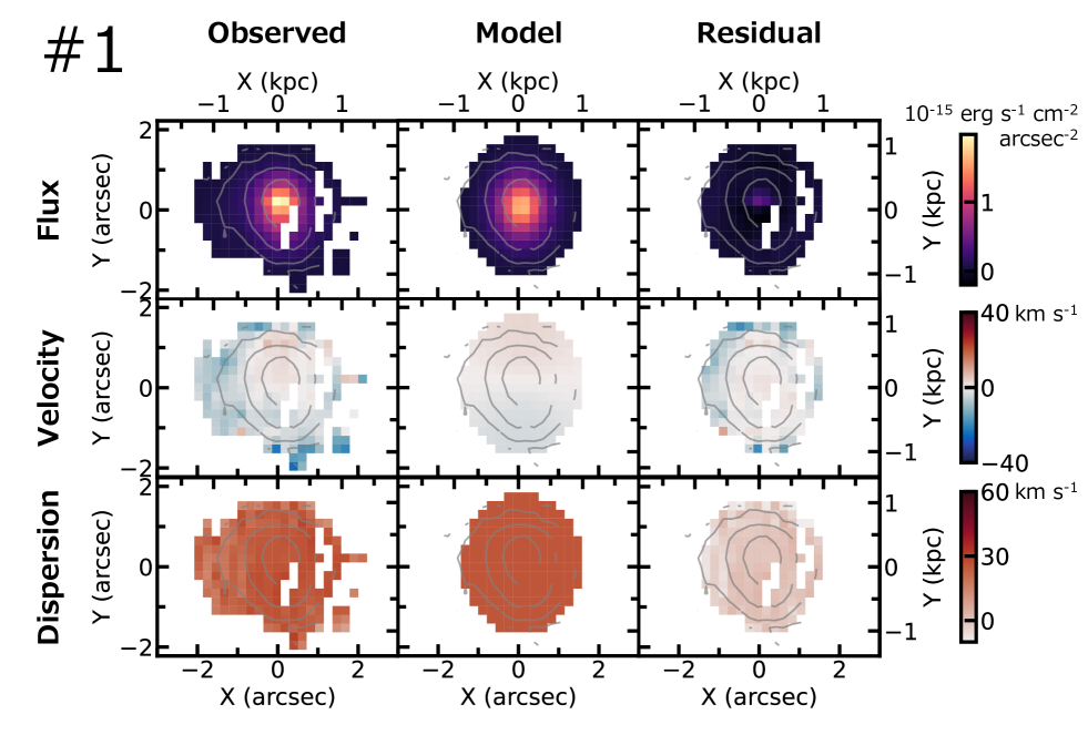
Figure 6: GalPaK^3D fitting of J1631+4426. The top, middle, and bottom panels show H$\alpha$ flux, velocity, and velocity-dispersion maps, respectively. The left, center, and right panels illustrate observed, model, and residual ($={\rm observed}-{\rm model}$) maps, respectively. Note that the velocity maps in this figure denote relative velocities with respect to the systemic redshift obtained with GalPaK^3D (Section 5.3).

Table 3: Morphological and additional kinematic properties of the 6 EMPGs

#	Name	$r_{\rm e,H\alpha}$	$i$	P.A.	$r_{\rm t}$
		pc	deg	deg	pc
(1)	(2)	(3)	(4)	(5)	(6)
1	J1631+4426	$248$	$44$	$178$	$61$
2	IZw18NW	$149$	$72$	$68$	$339$
3	SBS0335$-$052E	$211$	$25$	$320$	$258$
4	HS0822+3542	$33$	$41$	$91$	$1.1$
5	J1044+0353	$90$	$41$	$159$	$106$
6	J2115$-$1734	$176$	$43$	$222$	$387$

We conduct detailed dynamical modeling with the 3D parametric code GalPaK^3D (Bouché et al., 2015). Constraining morphological and kinematic properties simultaneously from 3D data cubes, GalPaK^3D provides the deprojected maximum rotational velocity ($v_{\rm rot}$) that is irrespective of the inclination. GalPaK^3D also calculates $\sigma_{0}$ free from the velocity dispersions driven by the self gravity (e.g., Genzel et al., 2008) or mixture of the line-of-sight velocities. Because GalPaK^3D does not support rectangular spaxels, we divide the spaxels in the Y direction based on the linear interpolation so that the pixel scale in the Y direction is the same as that in the X direction. We have 10 free parameters of XY coordinates of the disk center, systemic redshift, flux, inclination ($i$), position angle, effective radius of H$\alpha$ ($r_{\rm e,H\alpha}$), turnover radius ($r_{\rm t}$), $v_{\rm rot}$, and intrinsic velocity dispersion $\sigma_{0}$. We assume that all 6 EMPGs have thick disks with rotation curves of the arctan profiles:

$$v(r)=v_{\rm rot}\sin(i)\frac{2}{\pi}\arctan(r/r_{\rm t}),$$ (6)

where $r$ is a radius from the dynamical center. We note that $i$ is determined by the axis ratio and the disk height, where the disk height of the thick-disk model is fixed to $0.15r_{\rm e,H\alpha}$ (Bouché et al., 2015). We also assume that the surface-brightness (SB) profiles follow Sérsic profiles with Sérsic indices $n=1$, which are inferred from $i$-band SB profiles (Paper III). We have confirmed that these assumptions do not change $v_{\rm rot}$ and $\sigma_{0}$ much. We also use a point-spread function (PSF) obtained from standard stars with a Moffat profile whose FWHM and power index are $0.\!\!\arcsec 7$ and 2.5, respectively. Figure 6 summarizes fitting results. Table 2 lists kinematic properties extracted by the GalPaK^3D analysis. We estimate the errors of the $v_{\rm rot}$ and $\sigma_{0}$ values by carrying out the Monte Carlo simulations (Section 3.2). We note that $v_{\rm rot}$ can be regarded as an upper limit of the actual rotation velocity because the small-scale velocity differences in the complex velocity field can mimic rotation patterns (see also Section 5.2).

5.4 Mass Profile

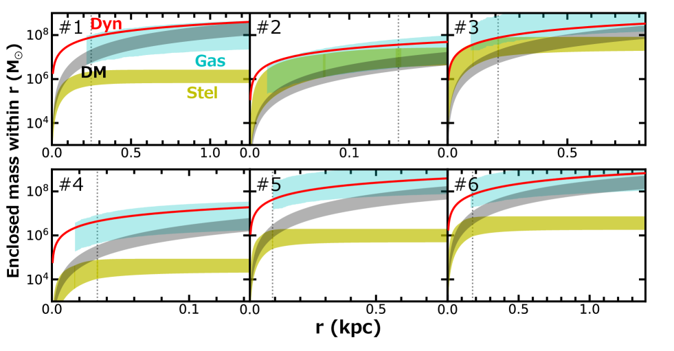
Figure 7: Enclosed mass profiles of the 6 EMPGs. The red, yellow, cyan, and black curves represent dynamical, stellar, gas, and dark-matter mass profiles, respectively. The vertical dotted lines show $r_{\rm e,H\alpha}$. The edge of the plots correspond to the outer most radii used for the kinematic analysis.

Table 4: Enclosed dynamical, stellar, gas, and DM masses, gas mass fraction, and Toomre $Q$

#	Name	$\log[M_{\rm dyn}(<r_{\rm e,H\alpha})]$	$\log[M_{*}(<r_{\rm e,H\alpha})]$	$\log[M_{\rm gas}(<r_{\rm e,H\alpha})]$	$\log[M_{\rm DM}(<r_{\rm e,H\alpha})]$	$f_{\rm gas}$	$Q$
		$M_{\odot}$	$M_{\odot}$	$M_{\odot}$	$M_{\odot}$
(1)	(2)	(3)	(4)	(5)	(6)	(7)	(8)
1	J1631+4426	$7.90\pm 0.06$	$6.0\pm 0.3$	$7.0^{+1.0}_{-0.3}$	$7.1\pm 0.3$	$0.91^{+0.06}_{-0.34}$	$5.1^{+2.1}_{-1.6}$
2	IZw18NW	$7.56\pm 0.02$	$7.0\pm 0.3$	$6.8^{+1.0}_{-0.3}$	$6.7\pm 0.3$	$0.42^{+0.38}_{-0.32}$	$11.6^{+56.7}_{-3.2}$
3	SBS0335$-$052E	$7.88\pm 0.02$	$7.4\pm 0.3$	$7.9^{+1.0}_{-0.3}$	$7.0\pm 0.3$	$0.74^{+0.17}_{-0.51}$	$2.6^{+4.7}_{-0.7}$
4	HS0822+3542	$6.64\pm 0.03$	$4.4\pm 0.3$	$5.9^{+1.0}_{-0.3}$	$5.2\pm 0.3$	$0.97^{+0.03}_{-0.07}$	$5.4^{+0.2}_{-2.5}$
5	J1044+0353	$7.63\pm 0.07$	$5.8\pm 0.3$	$7.5^{+1.0}_{-0.3}$	$6.2\pm 0.3$	$0.98^{+0.01}_{-0.09}$	$3.1^{+3.2}_{-0.0}$
6	J2115$-$1734	$7.86\pm 0.06$	$6.4\pm 0.3$	$7.6^{+1.0}_{-0.3}$	$6.8\pm 0.3$	$0.94^{+0.04}_{-0.18}$	$1.9^{+0.5}_{-0.6}$

The best-fit disk models obtained in Section 5.3 provide an estimate of the radial profiles for dynamical masses $M_{\rm dyn}$. The dynamical mass $M_{\rm dyn}$ is expected to be a sum of stellar mass $M_{*}$, gas mass $M_{\rm gas}$, dark-matter (DM) mass $M_{\rm DM}$, and dust mass $M_{\rm dust}$. Note that $M_{\rm dust}$ is negligible in all 6 EMPGs because of their low $E(B-V)$ values (e.g., Paper I). Hereafter, we derive radial profiles of $M_{\rm dyn}$, $M_{*}$, $M_{\rm gas}$, and $M_{\rm DM}$.

5.4.1 Dynamical mass profile

We derive $M_{\rm dyn}$ enclosed within the radius $r$ from the equation

$$M_{\rm dyn}(<r)=2.33\times 10^{5}\left(\frac{r}{\rm kpc}\right)\times\\ \left[\left(\frac{v(r)}{\rm km\ s^{-1}}\right)^{2}+2\left(\frac{\sigma_{0}}{\rm km\ s^{-1}}\right)^{2}\right]\ M_{\odot}$$ (7)

under the assumption of the virial equilibrium. Figure 7 presents mass profiles of all 6 EMPGs. The red curves correspond to $M_{\rm dyn}(<r)$. Dynamical masses within $r_{\rm e}$ are listed in Table 4.

5.4.2 Stellar mass profile

The stellar masses of 4 out of the 6 EMPGs (J1631+4426, J2115$-$1734, IZw18NW, and SBS0335$-$052E) are drawn from the literature (Paper I; Izotov & Thuan 1998; Izotov et al. 2009). For the other two targets (J1044+0353 and HS0822+3542), we provide here an estimate of their stellar mass.

We use the spectral energy distribution (SED) interpretation code of beagle (Chevallard & Charlot, 2016). The beagle code calculates both the stellar continuum and the nebular emission using the stellar population synthesis code (Bruzual & Charlot, 2003) and the nebular emission library of Gutkin et al. (2016) that are computed with the photoionization code cloudy (Ferland et al., 2013). We fit the SED models to SDSS $ugriz$-band photometries (DR16; Ahumada et al. 2020). We run the beagle code with 4 free parameters of maximum stellar age $t_{\rm max}$, stellar mass $M_{*}$, ionization parameter $U$, and $V$-band optical depth $\tau_{\rm V}$ whose parametric ranges are the same as those adopted in Papers III and IV. We fix metallicities $Z$ to be the gas-phase metallicities $12+\log(\rm O/H)$ listed in Table 1. We also assume a constant star-formation history and the Chabrier (2003) IMF in the same manner as Papers III and IV.

We note that we conduct the SED fitting with almost the same setting as that of Paper I for J1631+4426 and J2115$-$1734, except for $Z$ and $\tau_{\rm V}$. In Paper I, the $Z$ is treated as a free parameter, and the $\tau_{\rm V}$ is fixed to be 0, while it has no impact on $M_{*}$ of J1631+4426 and J2115$-$1734 because both 2 EMPGs are dust-poor (Paper I). We also confirm that the stellar masses of the 6 EMPGs are different only by $\lesssim 0.3$ dex from those derived from $i$-band magnitudes based on the same mass-to-light ratio. We include this systematic error of 0.3 dex into the total error of the $M_{*}$ profile.

To obtain $M_{*}$ profiles, we assume that azimuthally-averaged $M_{*}$ distributions of the EMPGs follow Sérsic profiles. J1631+4426 has an $i$-band effective radius ($r_{{\rm e},i}$) of $137^{+9}_{-7}$ pc and an $i$-band Sérsic index ($n_{i}$) of $1.08^{+0.15}_{-0.13}$ (Paper III). Because the $i$-band surface-brightness distribution is expected to trace the $M_{*}$ distribution well (Paper III), we assume that J1631+4426 has a stellar effective radius ($r_{\rm e,*}$) and a stellar Sérsic index ($n_{*}$) equal to $r_{{\rm e},i}$ and $n_{i}$, respectively. We also assume that the other 5 EMPGs have $r_{\rm e,*}$ within the range from $r_{\rm e,H\alpha}$/2 to $r_{\rm e,H\alpha}$ because $r_{{\rm e},i}$ of J1631+4426 is $\sim 2$ times smaller than $r_{\rm e,H\alpha}$ of J1631+4426 (see Table 3). We confirm that the assumed $r_{\rm e,*}$ of the 5 EMPGs are comparable to $r_{{\rm e},i}$ of EMPGs (Paper III). The 5 EMPGs are assumed to have $n_{*}$ within the range from 0.7 to 1.7 inferred from the typical $n_{i}$ value of EMPGs (Paper III). We include these uncertainties of $r_{\rm e,*}$ and $n_{*}$ into the error of the $M_{*}$ profile. The yellow shaded regions in Figure 7 represent cumulative $M_{*}$ profiles with their uncertainties. Stellar masses within $r_{\rm e}$ are listed in Table 4.

5.4.3 Gas mass profile

We obtain $M_{\rm gas}$ distributions from the H$\alpha$ flux distributions, using the Kennicutt-Schmidt law (Section 5.1). However, observational studies (e.g., Shi et al., 2014) have reported that some EMPGs have $\Sigma_{\rm gas}$ values $\sim 1$ dex larger than those inferred from the Kennicutt-Schmidt law, which can be interpreted as the lack of metals suppressing efficient gas cooling and succeeding star formation (e.g., Ostriker et al., 2010; Krumholz, 2013). Given the uncertainty of the Kennicutt-Schmidt law at the low-metallicity end, we add this 1 dex upper error to the original scatter of the Kennicutt-Schmidt law ($\sim 0.3$ dex; Kennicutt 1998). The cyan shaded regions in Figure 7 indicate cumulative $M_{\rm gas}$ profiles with their uncertainties. We note that the H i observations of Lelli et al. (2012) and Pustilnik et al. (2001) have reported that IZw18NW and SBS0335$-$052E have $M_{\rm gas}\sim 1\times 10^{8}$ and $\sim 1\times 10^{9}\ M_{\odot}$ within wide scales of $\sim 0.2$ and $\sim 3$ kpc, respectively, which are consistent with the extrapolations of the $M_{\rm gas}$ profiles that we derive. Gas masses within $r_{\rm e}$ are listed in Table 4. We obtain gas mass fractions at $r_{\rm e,H\alpha}$ from the following equation $f_{\rm gas}=M_{\rm gas}(<r_{\rm e,H\alpha})/[M_{\rm gas}(<r_{\rm e,H\alpha})+M_{*}(<r_{\rm e,H\alpha})]$.

5.4.4 Dark-matter mass profile

We estimate $M_{\rm DM}$ profiles under the assumption that the $M_{\rm DM}$ (density) profile follows the NFW profile (Navarro et al., 1996). At the virial radius $r_{200}$ within which the spherically-averaged mass density is 200 times the critical density $\rho_{\rm c}$, the NFW profile can be described by

$$\rho(r)=\rho_{\rm c}\frac{\delta}{c_{200}x(1+c_{200}x)^{2}},$$ (8)

where

$$\delta=\frac{200}{3}\frac{c_{200}^{3}}{\ln(1+c_{200})-c_{200}/(1+c_{200})}$$ (9)

and $x=r/r_{200}$. The concentration parameter $c_{200}$ is defined as the ratio $r_{200}/r_{\rm d}$ controlling where the slope equals $-2$ as it changes from $-3$ at large radii to a central value of $-1$. We obtain $r_{200}$ from the virial mass $M_{200}$ using the equation

$$r_{200}=\left[\frac{3M_{200}}{4\pi(200\rho_{\rm c})}\right]^{1/3}.$$ (10)

We derive $M_{200}$ from an empirical stellar-to-halo mass ratio of dwarf galaxies (Brook et al., 2014) of

$$M_{200}=7.96\times 10^{7}\left(\frac{M_{*}}{M_{\odot}}\right)^{1/3.1}\ M_{\odot}.$$ (11)

We note that the scatter of the observed stellar-to-halo mass ratios of dwarf galaxies around Equation 11 is $\sim 0.3$ dex (Prole et al., 2019). We include this uncertainty into the error of the $M_{\rm DM}$ profile. We also obtain $c_{200}$ from $M_{\rm 200}$ using a halo mass-concentration relation for the Planck cosmology (Dutton & Macciò, 2014):

$$\log(c_{200})=0.905-0.101\log(M_{200}/10^{12}h^{-1}M_{\odot}),$$ (12)

where $h=H_{0}/(100\ {\rm km}\ {\rm s}^{-1}\ {\rm Mpc}^{-1})$. The gray shaded regions in Figure 7 denote $M_{\rm DM}$ profiles with their uncertainties. DM masses within $r_{\rm e}$ are listed in Table 4.

6 Results

6.1 Rotation and Dispersion

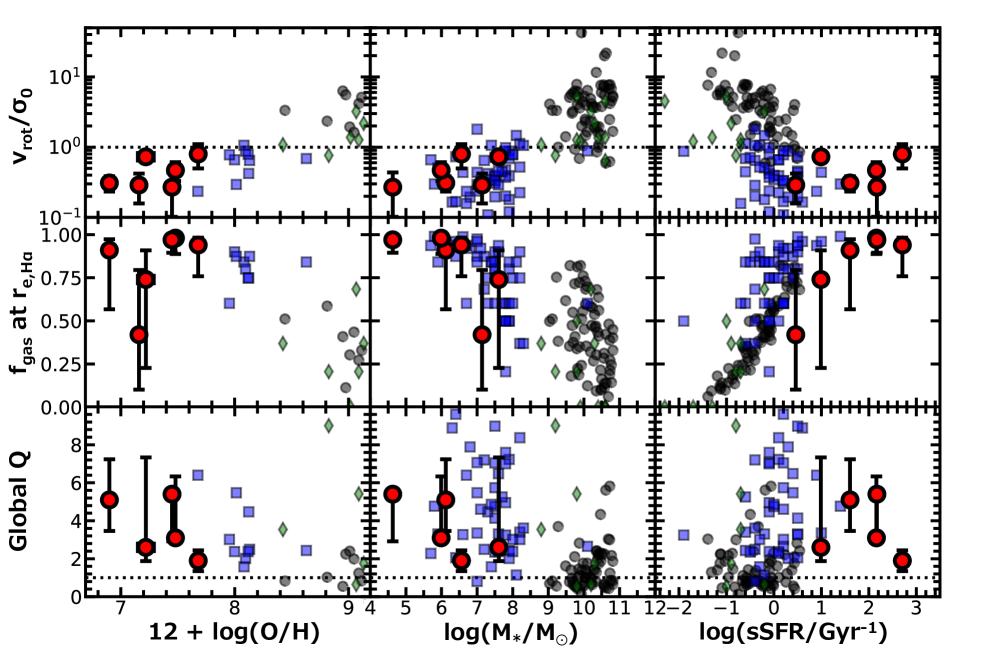
Figure 8: Diagrams of $v_{\rm rot}/\sigma_{0}$, $f_{\rm gas}$, and global $Q$ as functions of $12+\log(\rm O/H)$, $M_{*}$, and sSFR. The red circles represent the EMPGs, while the blue squares, the green diamonds, and the black circles indicate the SH$\alpha$DE (Barat et al., 2020), SAMI (Barat et al., 2019), and DYNAMO galaxies (Green et al., 2014), respectively. Because IZw18NW has the large uncertainty of the global $Q$ (see Table 4), we exclude the data point of this EMPG from the bottom panels.

Table 2 summarizes $v_{\rm shear}$, $\sigma_{\rm med}$, $v_{\rm rot}$, and $\sigma_{0}$ of the 6 EMPGs. Note that $v_{\rm shear}$ and $\sigma_{\rm med}$ ($v_{\rm rot}$ and $\sigma_{0}$) are based on the non-parametric (parametric) method explained in Section 5.2 (5.3). We find that all 6 EMPGs have low $v_{\rm shear}$ (5.5–14.3 km s^-1), high $\sigma_{\rm med}$ (16.9–30.8 km s^-1), and thus low $v_{\rm shear}/\sigma_{\rm med}$ (0.18–0.58). Regarding SBS0335$-$052E, Herenz et al. (2017) also obtain $v_{\rm shear}/\sigma_{\rm med}=0.68$, which is close to our measurement of $v_{\rm shear}/\sigma_{\rm med}=0.58\pm 0.02$. The 6 EMPGs also have low $v_{\rm rot}$ (4.5–23.4 km s^-1), high $\sigma_{0}$ (16.6–31.4 km s^-1), and low $v_{\rm rot}/\sigma_{0}$ (0.27–0.80). Using the 2 different methods, we confirm that all 6 EMPGs are dominated by dispersion (i.e., $v_{\rm shear}/\sigma_{\rm med}$, $v_{\rm rot}/\sigma_{0}<1$).

The top left panel of Figure 8 shows $v_{\rm rot}/\sigma_{0}$ values of the 6 EMPGs (red circle) as a function of metallicity. We compare our results with other surveys of H$\alpha$ kinematics of star-forming dwarf galaxies (SH$\alpha$DE; Barat et al. 2020) and star-forming galaxies (SAMI; Barat et al. 2019; DYNAMO; Green et al. 2014), whose metallicities are drawn from the SDSS MPA-JHU catalog (Tremonti et al., 2004; Brinchmann et al., 2004). The SH$\alpha$DE, SAMI, and DYNAMO galaxies have $12+\log(\rm O/H)\sim 8$–9. We find that $v_{\rm rot}/\sigma_{0}$ decreases with decreasing $12+\log(\rm O/H)$. The top middle and top right panels of Figure 8 show $v_{\rm rot}/\sigma_{0}$ as a function of $M_{*}$ and sSFR, respectively. The SFRs are derived from H$\alpha$ luminosity. The $M_{*}$ and sSFR potentially have uncertainties of $\sim 0.3$ dex under different assumptions such as initial mass functions (cf. Section 5.4.2). Although it should be noted that the EMPGs are biased toward lower metallicities, we also find that $v_{\rm rot}/\sigma_{0}$ decreases as $M_{*}$ decreases and sSFR increases. These results suggest that galaxies in earlier stages of the formation phase may have lower $v_{\rm rot}/\sigma_{0}$.

6.2 Mass Fraction

Figure 7 summarizes radial profiles of $M_{\rm dyn}$ (red), $M_{*}$ (yellow), $M_{\rm gas}$ (cyan), and $M_{\rm DM}$ (black). We find that the 4 EMPGs other than IZw18NW or SBS0335$-$052E have the $M_{*}$ profiles $\sim 2$ dex below the $M_{\rm dyn}$ profiles within radii up to several times $r_{\rm e,H\alpha}$, which means that the 4 EMPGs are dominated by $M_{\rm gas}$ or $M_{\rm DM}$ on galactic scales. On the other hand, IZw18NW and SBS0335$-$052E have the $M_{*}$ profiles comparable to the $M_{\rm dyn}$ profiles. We also find that the $M_{\rm dyn}$ profiles of all 6 EMPGs can be explained by the $M_{\rm gas}$ profiles within the uncertainties (see Section 5.4.3). We confirm that the $M_{\rm DM}$ profiles of all 6 EMPGs are $\sim 1$ dex below the $M_{\rm dyn}$ profiles within radii up to several times $r_{\rm e,H\alpha}$. We thus conclude that the masses of the 4 EMPGs except for IZw18NW and SBS0335$-$052E are dominated by $M_{\rm gas}$ on galactic scales. We note that IZw18NW and SBS0335$-$052E indeed have large $M_{\rm gas}$ values of $\sim 1\times 10^{8}$ and $\sim 1\times 10^{9}\ M_{\odot}$ inferred from the H i observations within $\sim 0.2$ and $\sim 3$ kpc, respectively (Section 5.4.3). Within these larger scales, we can say that both IZw18NW and SBS0335$-$052E are gas-rich (i.e., $f_{\rm gas}\sim 1$). This conclusion is consistent with those in Pustilnik et al. (2020a, b, 2021) based on H i observations. It should also be noted that Equations 10 and 11 suggest that EMPGs with $\sim 10^{6}\ M_{\odot}$ have $M_{200}\sim 7\times 10^{9}\ M_{\odot}$ at $r_{200}\sim 30$ kpc, whereas we can only observe the area within at most $\sim 1$ kpc. Therefore, it is natural that $M_{\rm DM}$ has negligible effects on the mass profile in this study.

The middle left panel of Figure 8 shows $f_{\rm gas}$ of the 6 EMPGs as a function of metallicity. Except for IZw18NW and SBS0335$-$052E with large $f_{\rm gas}$ uncertainties, we find that the EMPGs are gas-rich with high $f_{\rm gas}$ values of $\sim 0.9$–1.0. Comparing with the literature, we find that galaxies with lower metallicities tend to have higher $f_{\rm gas}$ values. The $f_{\rm gas}$ values also increase at lower $M_{*}$ and higher sSFR. These results indicate that galaxies in the earlier formation phase would have higher $f_{\rm gas}$, which are consistent with previous observations (e.g., Maseda et al., 2014) as well as models of galaxy formation based on the $\Lambda$CDM model (e.g., Geach et al., 2011). It should be noted that $M_{\rm gas}$ of the SH$\alpha$DE and DYNAMO galaxies are estimated from Kennicutt-Schmidt law (i.e., correlation between $\Sigma_{\rm SFR}$ and $\Sigma_{\rm gas}$) in the similar way as our analysis (cf. Section 5.4.3). Thus, it is natural that we find a tight correlation between sSFR and $f_{\rm gas}$.

7 Discussion

7.1 Origin of Low $v_{\rm rot}/\sigma_{0}$

In Section 6.1, we report that all 6 EMPGs have low $v_{\rm rot}/\sigma_{0}<1$. We also find that $v_{\rm rot}/\sigma_{0}$ decreases with decreasing $12+\log(\rm O/H)$, decreasing $M_{*}$, and increasing sSFR (Figure 8). Below, we investigate well-discussed three contributors (e.g., Glazebrook, 2013; Barat et al., 2020) to such a low $v_{\rm rot}/\sigma_{0}<1$.

7.1.1 Thermal expansion

The first possible contributor to the low $v_{\rm rot}/\sigma_{0}$ is the thermal expansion of H ii regions (e.g., Krumholz et al., 2018; Fukushima & Yajima, 2021, 2022). We estimate a velocity dispersion of the thermal expansion ($\sigma_{\rm th}$) from the line-of-sight component of the Maxwellian velocity distribution ($\sigma_{\rm th}=\sqrt{kT_{\rm e}/m}$; e.g., Chávez et al. 2014; Pillepich et al. 2019), where $k$, $T_{\rm e}$, and $m$ represent the Boltzmann constant, the electron temperature, and the hydrogen mass, respectively. We obtain $\sigma_{\rm th}={\color[rgb]{0,0,0}9.1}$ km s^-1 under the assumption of $T_{\rm e}=10000$ K, which is consistent with the typical electron temperature of O ii (i.e., H ii) regions of the EMPGs (e.g., Paper I). Subtracting $\sigma_{\rm th}$ from $\sigma_{0}$ quadratically, we obtain velocity dispersions being free from the thermal line broadening ($\sigma_{\rm no\_therm}={\color[rgb]{0,0,0}14}$–30 km s^-1). We confirm that $v_{\rm rot}/\sigma_{\rm no\_therm}$ values are still lower than unity (0.31–0.84) for all 6 EMPGs. We thus conclude that the thermal expansion cannot explain $v_{\rm rot}/\sigma_{0}<1$.

7.1.2 Merger/inflow

The second possible contributor is merger/inflow events (e.g., Glazebrook, 2013). The merger (inflow) can raise velocity dispersions by tidal heating (releasing potential energies of infalling gas). This scenario can explain all the trends seen in Figure 8 because we can expect that both gas-rich minor merger and inflow would supply metal-poor gas and trigger succeeding starbursts. Especially for J1631+4426, IZw18NW, SBS0335$-$052E, and J2115$-$1734, we find the velocity differences from the EMPG tails (IZw18SE for IZw18NW) suggestive of merger (Section 4).

7.1.3 Stellar feedback

The third possible contributor is the stellar feedback (e.g., Lehnert et al., 2009). This includes the supernova (SN) feedback (Dib et al., 2006) as well as stellar winds and the radiative pressure from young massive stars (Mac Low & Klessen, 2004). Outflowing gas from SNe and/or young massive stars would raise velocity dispersions. This stellar feedback scenario can directly explain the decreasing trend between $v_{\rm rot}/\sigma_{0}$ and sSFR (the top right panel of Figure 8). Given the expectation that young galaxies (i.e., with high sSFRs) would have low $12+\log(\rm O/H)$ and $M_{*}$, this scenario can indirectly reproduce the trend that $v_{\rm rot}/\sigma_{0}$ decreases with decreasing $12+\log(\rm O/H)$ and $M_{*}$. IZw18NW, SBS0335$-$052E, and J1044+0353 especially show outflow signatures in flux, velocity, and velocity-dispersion maps (see Section 4), which imply the dominance of the stellar feedback. We thus conclude that the stellar feedback can also be one of the main contributors of $v_{\rm rot}/\sigma_{0}<1$ at the low-metallicity, low-$M_{*}$, and high-sSFR ends. Cosmological zoom-in simulations will provide a hint of what kind of feedback is the main contributor.

7.2 Toomre Q Parameter

To compare with other kinematic studies, we derive the Toomre $Q$ parameter (Toomre, 1964) of the EMPGs. In general, if the $Q$ value of a rotating disk is greater than unity (i.e., $Q>1$), the disk is thought to be gravitationally stable. On the other hand, the disk is gravitationally unstable if $Q<1$. However, note that it is unclear if this criterion is applicable for the EMPGs because they may not have rotating disks (Section 4). An average of $Q$ within a disk so called the global $Q$ (e.g., Aumer et al., 2010) is calculated from the equation

$$Q=\frac{\sigma_{0}}{v_{\rm rot}}\frac{a}{f_{\rm gas}},$$ (13)

where $a$ is a parameter with values ranging from 1 to 2 depending on the gas distribution (Genzel et al., 2011). Here, we adopt $a=\sqrt{2}$ assuming the constant rotational velocity.

Table 4 lists the global $Q$ of the 6 EMPGs. We find that all the 6 EMPGs show $Q>1$, albeit one of the 6 EMPGs (IZw18NW) with the large $Q$ uncertainty. The bottom panels of Figure 8 illustrate the global $Q$ of the EMPGs as a function of metallicity (bottom left), $M_{*}$ (bottom center), and sSFR (bottom right), while we exclude IZw18NW due to its large $Q$ uncertainty. We also find that the global $Q$ increases with decreasing $12+\log(\rm O/H)$, decreasing $M_{*}$, and increasing sSFR. However, the large global $Q$ values are inconsistent with the large sSFR values because star-formation activities are not likely to become aggressive in a gravitationally-stable disk.

This inconsistency probably originates from the fact that the global $Q$ parameter is not a reliable indicator for gas-rich galaxies (Romeo et al., 2010; Romeo & Agertz, 2014). Instead, it can be important to investigate if the EMPGs lie on a tight relation based on observables such as H i angular momentum (Romeo, 2020; Romeo et al., 2020). We need high-resolution H i observations to discuss gravitational instability of EMPGs precisely.

7.3 Connection to High-$z$ Primordial Galaxies

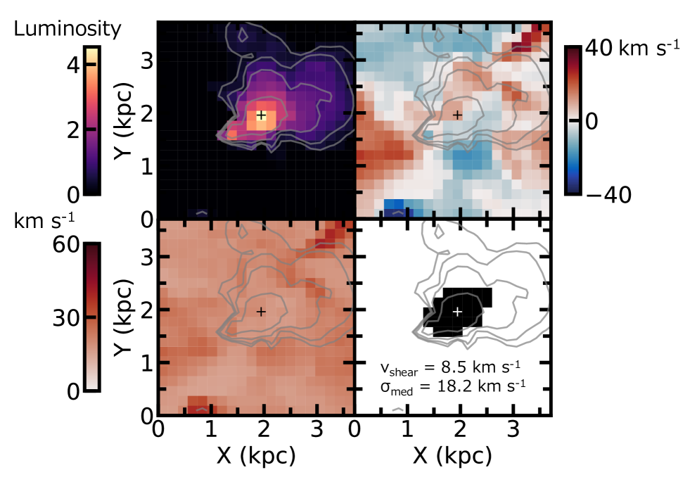
Figure 9: H$\alpha$ luminosity (top left), velocity (top right), velocity-dispersion (bottom left), and mask maps (bottom right) of the $z=7.3$ primordial galaxy in Wise et al. (2014). The luminosity is in units of $10^{35}$ erg s^-1 Å^-1 in log scale. The maximum luminosity value ($7\times 10^{39}$ erg s^-1 Å^-1) corresponds to a flux of $3\times 10^{-15}$ erg s^-1 cm^-2 Å^-1 at $z=0.03125$. The gray contours illustrate H$\alpha$ luminosity values in the order of 1/16, 1/8, 1/4, and 1/2 of the maximum luminosity value.

The trend that $v_{\rm rot}/\sigma_{0}$ ($f_{\rm gas}$) decreases (increases) with decreasing (increasing) $12+\log(\rm O/H)$ and $M_{*}$ (sSFR) suggests that primordial galaxies at high redshifts would be dispersion-dominated gas-rich systems. This suggestion agrees with the decreasing trend of $v_{\rm rot}/\sigma_{0}$ with the redshift reported by both observational (e.g., Wisnioski et al., 2015) and simulation (Pillepich et al., 2019) studies.

Here, we investigate kinematics of simulated primordial galaxies at high redshifts. In this study, we choose a $z=7.3$ primordial galaxy of Wise et al. (2014)’s cosmological radiation hydrodynamics simulation because the simulated galaxy has a low gas-phase metallicity ($\sim 4$% $Z_{\odot}$), a low stellar mass ($3.8\times 10^{6}\ M_{\odot}$), a large $f_{\rm gas}$ ($\sim 1$), a large sSFR ($\sim 5$ Gyr^-1), and a small half-mass radius ($\sim 200$ pc), all of which are comparable to those of the EMPGs (Sections 2 and 5.4.2). Wise et al. in prep. (hereafter W23) extract H$\alpha$ flux, velocity, and velocity-dispersion maps from the simulated galaxy. The FoV of the extracted region is 3.71 kpc with the spatial resolution of $3.71/252=0.015$ kpc pixel^-1. The spectral resolution of the datacube is 0.1 Å. W23 use cloudy (Ferland et al., 2013) to derive H$\alpha$ fluxes from the following 5 quantities: Hydrogen number density, temperature, metallicity, incident radiation intensity, and H i column density, along with enough parametric ranges and number of datapoints (1.8 million points in total). For each cell in the data cube of the 5 quantities, W23 linearly interpolate the emissivity table in 5D. To calculate the velocity map, W23 sum the line-of-sight velocities weighted by the H-alpha fluxes. To calculate the velocity dispersion map, W23 use the same method as Pillepich et al. (2019; Equation A3), using the H-alpha flux as the weights. We note that the velocity dispersions include the thermal broadening.

We coarsen the data cube to a spatial resolution of 180 pc, similar to the resolution of our observations, to make a more relevant comparison. The top left, top right, and bottom left panels of Figure 9 are H$\alpha$ flux, velocity, and velocity-dispersion maps of the simulated galaxy, respectively. We find that the simulated galaxy has an irregular morphology with multiple kinematic sub-structures and localized turbulent regions. These features can be seen in the EMPGs as well (Figure 4). Masking out the kinematic sub-structures and the turbulent regions, we also derive kinematics properties of $v_{\rm shear}$ and $\sigma_{\rm med}$ in the same manner as we do for the EMPGs (Sections 5.1 and 5.2). We find that the simulated galaxy has a low $v_{\rm shear}$ (8.5 km s^-1) and a high $\sigma_{\rm med}$ (18.2 km s^-1), which are comparable to those of the EMPGs ($v_{\rm shear}=5.5$–14.3 km s^-1, $\sigma_{\rm med}=16.9$–30.8 km s^-1; see Section 6.1). Consequently, the simulated galaxy has a low $v_{\rm shear}/\sigma_{\rm med}=0.47$ below unity suggesting that the simulated galaxy is dominated by dispersion as well as the EMPGs. Given that the local EMPGs, analogs of high-$z$ primordial galaxies, and the simulated high-$z$ primordial galaxies are both dispersion-dominated systems, we expect that high-$z$ primordial galaxies are likely to be dispersion-dominated galaxies.

The forthcoming James Webb Space Telescope (JWST) can directly investigate H$\alpha$ kinematics of high-$z$ primordial galaxies. Paper IV has simulated H$\alpha$ fluxes of primordial galaxies with $M_{*}=10^{6}\ M_{\odot}$ at redshifts ranging from 0 to 10. Comparing the H$\alpha$ fluxes with the limiting flux of JWST/NIRSpec, we estimate that NIRSpec can detect H$\alpha$ fluxes of primordial galaxies with $M_{*}=10^{6}\ M_{\odot}$ at $z\lesssim 1$ without gravitational lensing. With a $\sim 2$ dex magnification from gravitational lensing, NIRSpec can detect H$\alpha$ fluxes of primordial galaxies with $M_{*}=10^{6}\ M_{\odot}$ at $z\sim{\color[rgb]{0,0,0}7}$. We infer from this estimation that NIRSpec could observe primordial galaxies with $M_{*}\sim 10^{7}\ M_{\odot}$ at $z\sim 7$ with a realistic magnification of $\sim 1$ dex. The top middle panel of Figure 8 shows that most of galaxies with $M_{*}\sim 10^{7}\ M_{\odot}$ already have low $v_{\rm rot}/\sigma_{0}<1$ and high $f_{\rm gas}>0.5$. Lensing cluster surveys using JWST such as GLASS (PI: T. Treu) and CANUCS (PI: C. Willott) will potentially pinpoint low-mass galaxies with $M_{*}\sim 10^{7}\ M_{\odot}$ at $z\sim 7$, and follow-up IFU observations with JWST may identify dispersion-dominated gas-rich galaxies.

8 Summary

We present kinematics of 6 local extremely metal-poor galaxies (EMPGs) with low metallicities ($0.016-0.098\ Z_{\odot}$) and low stellar masses ($10^{4.7}-10^{7.6}M_{\odot}$; Section 2). Taking deep medium-high resolution ($R\sim 7500$) integral-field spectra with 8.2-m Subaru (Section 3), we resolve the small inner velocity gradients and dispersions of the EMPGs with H$\alpha$ emission. Carefully masking out sub-structures originated by inflow and/or outflow, we fit 3-dimensional disk models to the observed H$\alpha$ flux, velocity, and velocity-dispersion maps (Sections 4 and 5). All the EMPGs show rotational velocities ($v_{\rm rot}$) of 5–23 km s^-1 smaller than the velocity dispersions ($\sigma_{0}$) of 17–31 km s^-1, indicating dispersion-dominated systems with small ratios of $v_{\rm rot}/\sigma_{0}=0.29-0.80$ (Section 6.1) that can be explained by turbulence driven by inflow and/or outflow (Section 7.1). Except for two EMPGs with large uncertainties, we find that the EMPGs have very large gas-mass fractions of $f_{\rm gas}\simeq 0.9-1.0$ (Section 6.2). Comparing our results with other H$\alpha$ kinematics studies, we find that $v_{\rm rot}/\sigma_{0}$ ($f_{\rm gas}$) decreases (increases) with decreasing metallicity. We compare numerical simulations of first-galaxy formation and identify that the simulated high-$z$ ($z\sim 7$) forming galaxies have gas-fractions and dynamics similar to the observed EMPGs. Our EMPG observations and the simulations suggest that primordial galaxies are gas-rich dispersion-dominated systems, which would be identified by the forthcoming JWST observations at $z\sim 7$ (Section 7.3).

We are grateful to Yoshiaki Sofue, Alessandro Romeo, and Roberto Terlevich for having useful discussions. We also thank the staff of Subaru Telescope for their help with the observations. This research is based on data collected at the Subaru Telescope, which is operated by the National Astronomical Observatory of Japan (NAOJ). We are honored and grateful for the opportunity of observing the Universe from Maunakea, which has the cultural, historical, and natural significance in Hawaii. The Hyper Suprime-Cam (HSC) collaboration includes the astronomical communities of Japan and Taiwan, and Princeton University. The HSC instrumentation and software were developed by the NAOJ, the Kavli Institute for the Physics and Mathematics of the Universe (Kavli IPMU), the University of Tokyo, the High Energy Accelerator Research Organization (KEK), the Academia Sinica Institute for Astronomy and Astrophysics in Taiwan (ASIAA), and Princeton University. Based on data collected at the Subaru Telescope and retrieved from the HSC data archive system, which is operated by Subaru Telescope and Astronomy Data Center at NAOJ. This work was supported by the joint research program of the Institute for Cosmic Ray Research (ICRR), University of Tokyo. Y.I., K. Nakajima, Y.H., T.K., and M. Onodera are supported by JSPS KAKENHI Grant Nos. 21J20785, 20K22373, 19J01222, 18J12840, and 21K03622, respectively. K.H. is supported by JSPS KAKENHI Grant Nos. 20H01895, 21K13909, and 21H05447. Y.H. is supported by JSPS KAKENHI Grant Nos. 21J00153, 20K14532, 21H04499, 21K03614, and 22H01259. H.Y. is supported by MEXT / JSPS KAKENHI Grant Number 21H04489 and JST FOREST Program, Grant Number JP-MJFR202Z. J.H.K acknowledges the support from the National Research Foundation of Korea (NRF) grant, No. 2020R1A2C3011091 and No. 2021M3F7A1084525, funded by the Korea government (MSIT). This work has been supported by the Japan Society for the Promotion of Science (JSPS) Grants-in-Aid for Scientific Research (19H05076 and 21H01128). This work has also been supported in part by the Sumitomo Foundation Fiscal 2018 Grant for Basic Science Research Projects (180923), and the Collaboration Funding of the Institute of Statistical Mathematics “New Development of the Studies on Galaxy Evolution with a Method of Data Science”. The Cosmic Dawn Center is funded by the Danish National Research Foundation under grant No. 140. S.F. acknowledges support from the European Research Council (ERC) Consolidator Grant funding scheme (project ConTExt, grant No. 648179). This project has received funding from the European Union’s Horizon 2020 research and innovation program under the Marie Sklodowska-Curie grant agreement No. 847523 “INTERACTIONS”. This work is supported by World Premier International Research Center Initiative (WPI Initiative), MEXT, Japan, as well as KAKENHI Grant-in-Aid for Scientific Research (A) (15H02064, 17H01110, 17H01114, 20H00180, and 21H04467) through Japan Society for the Promotion of Science (JSPS). This work has been supported in part by JSPS KAKENHI Grant Nos. JP17K05382, JP20K04024, and JP21H04499 (K. Nakajima). This research was supported by a grant from the Hayakawa Satio Fund awarded by the Astronomical Society of Japan. JHW acknowledges support from NASA grants NNX17AG23G, 80NSSC20K0520, and 80NSSC21K1053 and NSF grants OAC-1835213 and AST-2108020.

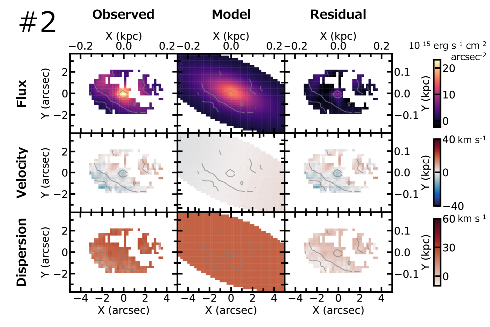
Figure 10: GalPaK^3D result of IZw18NW.

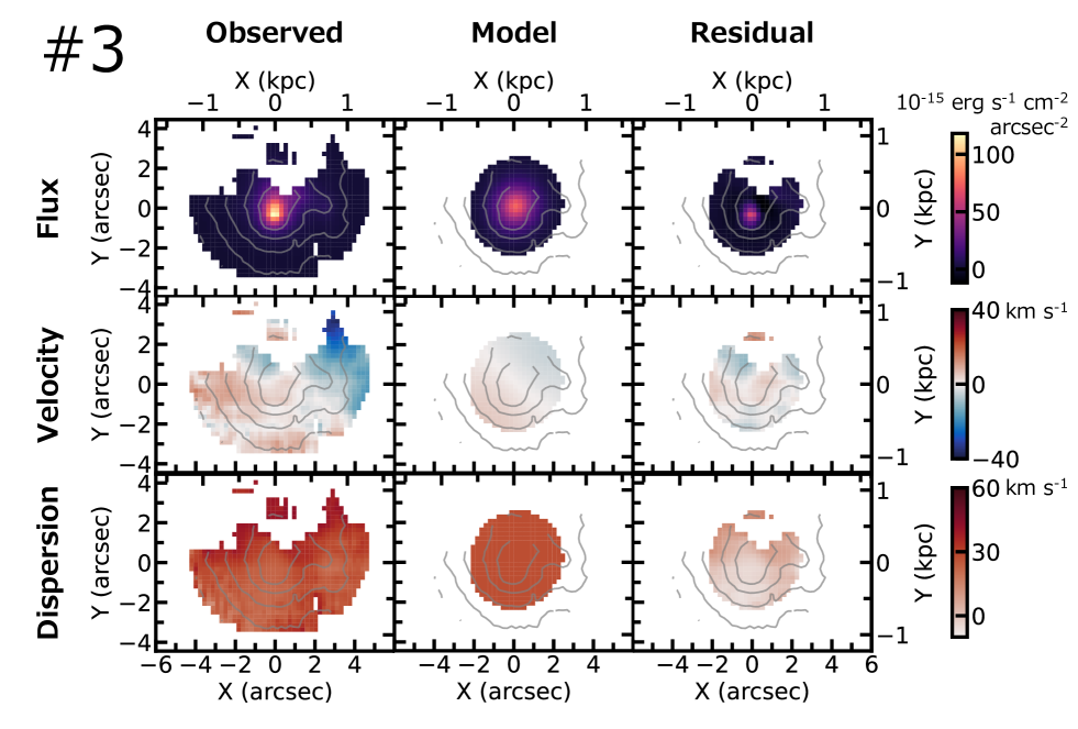
Figure 11: GalPaK^3D result of SBS0335$-$052E.

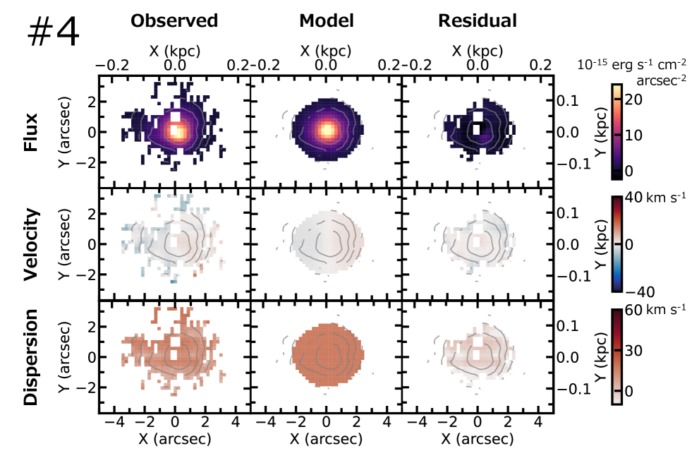
Figure 12: GalPaK^3D result of HS0822+3542.

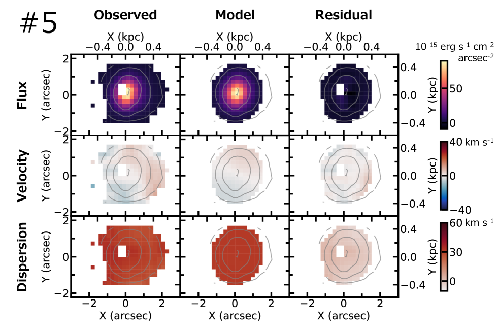
Figure 13: GalPaK^3D result of J1044+0353.

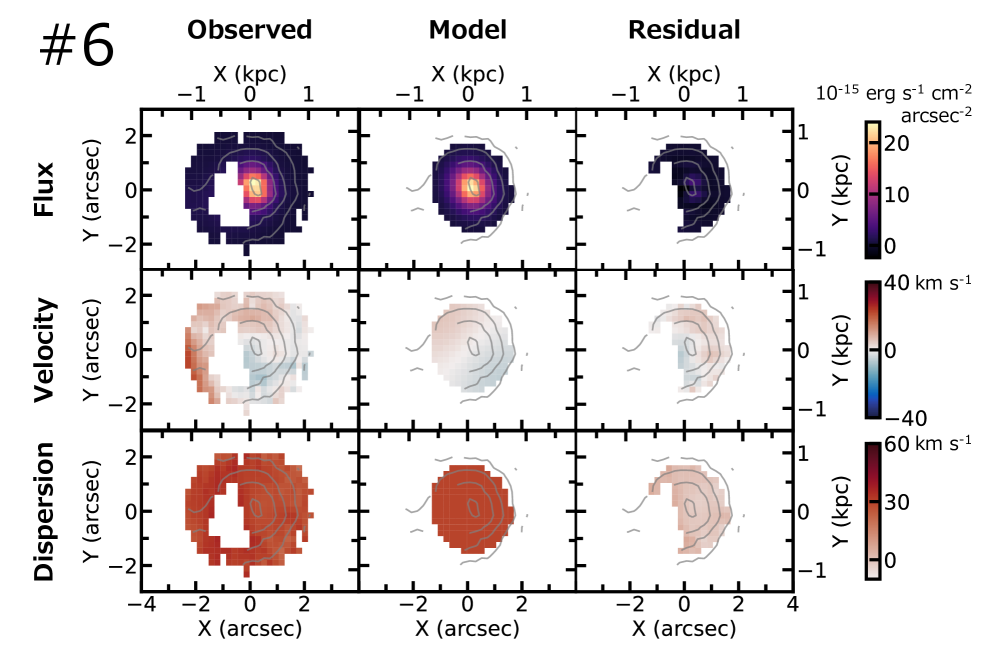
Figure 14: GalPaK^3D result of J2115$-$1734.

Figures 10–14 show GalPaK^3D fitting results of the 5 EMPGs other than J1631+4426.

References

- Ahumada et al. (2020) Ahumada, R., Prieto, C. A., Almeida, A., et al. 2020, ApJS, 249, 3, doi: 10.3847/1538-4365/ab929e
- Aihara et al. (2019) Aihara, H., AlSayyad, Y., Ando, M., et al. 2019, PASJ, 71, 114, doi: 10.1093/pasj/psz103
- Aihara et al. (2022) —. 2022, PASJ, 74, 247, doi: 10.1093/pasj/psab122
- Annibali et al. (2013) Annibali, F., Cignoni, M., Tosi, M., et al. 2013, AJ, 146, 144, doi: 10.1088/0004-6256/146/6/144
- Asplund et al. (2021) Asplund, M., Amarsi, A. M., & Grevesse, N. 2021, A&A, 653, A141, doi: 10.1051/0004-6361/202140445
- Astropy Collaboration et al. (2013) Astropy Collaboration, Robitaille, T. P., Tollerud, E. J., et al. 2013, A&A, 558, A33, doi: 10.1051/0004-6361/201322068
- Aumer et al. (2010) Aumer, M., Burkert, A., Johansson, P. H., & Genzel, R. 2010, ApJ, 719, 1230, doi: 10.1088/0004-637X/719/2/1230
- Bacon et al. (1995) Bacon, R., Adam, G., Baranne, A., et al. 1995, A&AS, 113, 347
- Barat et al. (2020) Barat, D., D’Eugenio, F., Colless, M., et al. 2020, MNRAS, 498, 5885, doi: 10.1093/mnras/staa2716
- Barat et al. (2019) —. 2019, MNRAS, 487, 2924, doi: 10.1093/mnras/stz1439
- Berg et al. (2016) Berg, D. A., Skillman, E. D., Henry, R. B. C., Erb, D. K., & Carigi, L. 2016, ApJ, 827, 126, doi: 10.3847/0004-637X/827/2/126
- Bouché et al. (2015) Bouché, N., Carfantan, H., Schroetter, I., Michel-Dansac, L., & Contini, T. 2015, AJ, 150, 92, doi: 10.1088/0004-6256/150/3/92
- Brinchmann et al. (2004) Brinchmann, J., Charlot, S., White, S. D., et al. 2004, MNRAS, doi: 10.1111/j.1365-2966.2004.07881.x
- Brook et al. (2014) Brook, C. B., Cintio, A. D., Knebe, A., et al. 2014, ApJL, 784, 1, doi: 10.1088/2041-8205/784/1/L14
- Bruzual & Charlot (2003) Bruzual, G., & Charlot, S. 2003, MNRAS, 344, 1000, doi: 10.1046/j.1365-8711.2003.06897.x
- Chabrier (2003) Chabrier, G. 2003, PASP, 115, 763, doi: 10.1086/376392
- Chávez et al. (2014) Chávez, R., Terlevich, R., Terlevich, E., et al. 2014, MNRAS, 442, 3565, doi: 10.1093/mnras/stu987
- Chevallard & Charlot (2016) Chevallard, J., & Charlot, S. 2016, MNRAS, 462, 1415, doi: 10.1093/mnras/stw1756
- Dib et al. (2006) Dib, S., Bell, E., & Burkert, A. 2006, ApJ, 638, 797, doi: 10.1086/498857
- Dufour & Hester (1990) Dufour, R. J., & Hester, J. J. 1990, ApJ, 350, 149, doi: 10.1086/168369
- Dutton & Macciò (2014) Dutton, A. A., & Macciò, A. V. 2014, MNRAS, 441, 3359, doi: 10.1093/mnras/stu742
- Egorov et al. (2021) Egorov, O. V., Lozinskaya, T. A., Vasiliev, K. I., et al. 2021, MNRAS, 508, 2650, doi: 10.1093/mnras/stab2710
- Ferland et al. (2013) Ferland, G. J., Porter, R. L., van Hoof, P. A. M., et al. 2013, Rev. Mexicana Astron. Astrofis., 49, 137. https://arxiv.org/abs/1302.4485
- Flewelling et al. (2020) Flewelling, H. A., Magnier, E. A., Chambers, K. C., et al. 2020, ApJS, 251, 7, doi: 10.3847/1538-4365/abb82d
- Förster Schreiber et al. (2009) Förster Schreiber, N. M., Genzel, R., Bouché, N., et al. 2009, ApJ, 706, 1364, doi: 10.1088/0004-637X/706/2/1364
- Fukushima & Yajima (2021) Fukushima, H., & Yajima, H. 2021, MNRAS, 506, 5512, doi: 10.1093/mnras/stab2099
- Fukushima & Yajima (2022) —. 2022, MNRAS, 511, 3346, doi: 10.1093/mnras/stac244
- Geach et al. (2011) Geach, J. E., Smail, I., Moran, S. M., et al. 2011, ApJ, 730, L19, doi: 10.1088/2041-8205/730/2/L19
- Genzel et al. (2008) Genzel, R., Burkert, A., Bouché, N., et al. 2008, ApJ, 687, 59, doi: 10.1086/591840
- Genzel et al. (2011) Genzel, R., Newman, S., Jones, T., et al. 2011, ApJ, 733, doi: 10.1088/0004-637X/733/2/101
- Glazebrook (2013) Glazebrook, K. 2013, PASA, 30, e056, doi: 10.1017/pasa.2013.34
- Green et al. (2014) Green, A. W., Glazebrook, K., McGregor, P. J., et al. 2014, MNRAS, 437, 1070, doi: 10.1093/mnras/stt1882
- Gutkin et al. (2016) Gutkin, J., Charlot, S., & Bruzual, G. 2016, MNRAS, 462, 1757, doi: 10.1093/mnras/stw1716
- Herenz et al. (2017) Herenz, E. C., Hayes, M., Papaderos, P., et al. 2017, A&A, 606, L11, doi: 10.1051/0004-6361/201731809
- Herenz et al. (2016) Herenz, E. C., Gruyters, P., Orlitova, I., et al. 2016, A&A, 587, A78, doi: 10.1051/0004-6361/201527373
- Herrera-Camus et al. (2022) Herrera-Camus, R., Förster Schreiber, N. M., Price, S. H., et al. 2022, arXiv e-prints, arXiv:2203.00689. https://arxiv.org/abs/2203.00689
- Hirschauer et al. (2016) Hirschauer, A. S., Salzer, J. J., Skillman, E. D., et al. 2016, ApJ, 822, 108, doi: 10.3847/0004-637X/822/2/108
- Hsyu et al. (2017) Hsyu, T., Cooke, R. J., Prochaska, J. X., & Bolte, M. 2017, ApJ, 845, L22, doi: 10.3847/2041-8213/aa821f
- Isobe et al. (2021) Isobe, Y., Ouchi, M., Kojima, T., et al. 2021, ApJ, 918, 54, doi: 10.3847/1538-4357/ac05bf
- Isobe et al. (2022) Isobe, Y., Ouchi, M., Suzuki, A., et al. 2022, ApJ, 925, 111, doi: 10.3847/1538-4357/ac3509
- Izotov et al. (2009) Izotov, Y. I., Guseva, N. G., Fricke, K. J., & Papaderos, P. 2009, A&A, 503, 61, doi: 10.1051/0004-6361/200911965
- Izotov et al. (1997) Izotov, Y. I., Lipovetsky, V. A., Chaffee, F. H., et al. 1997, ApJ, 476, 698, doi: 10.1086/303664
- Izotov et al. (2006) Izotov, Y. I., Stasińska, G., Meynet, G., Guseva, N. G., & Thuan, T. X. 2006, A&A, 448, 955, doi: 10.1051/0004-6361:20053763
- Izotov & Thuan (1998) Izotov, Y. I., & Thuan, T. X. 1998, ApJ, 497, 227, doi: 10.1086/305440
- Izotov et al. (2012) Izotov, Y. I., Thuan, T. X., & Guseva, N. G. 2012, A&A, doi: 10.1051/0004-6361/201219733
- Izotov et al. (2018) Izotov, Y. I., Thuan, T. X., Guseva, N. G., & Liss, S. E. 2018, MNRAS, doi: 10.1093/mnras/stx2478
- Kashikawa et al. (2002) Kashikawa, N., Aoki, K., Asai, R., et al. 2002, PASJ, 54, 819, doi: 10.1093/pasj/54.6.819
- Kashiwagi et al. (2021) Kashiwagi, Y., Inoue, A. K., Isobe, Y., et al. 2021, PASJ, 73, 1631, doi: 10.1093/pasj/psab100
- Kennicutt (1998) Kennicutt, Robert C., J. 1998, ApJ, 498, 541, doi: 10.1086/305588
- Kikuchihara et al. (2020) Kikuchihara, S., Ouchi, M., Ono, Y., et al. 2020, ApJ, 893, 60, doi: 10.3847/1538-4357/ab7dbe
- Kniazev et al. (2003) Kniazev, A. Y., Grebel, E. K., Hao, L., et al. 2003, ApJ, 593, L73, doi: 10.1086/378259
- Kniazev et al. (2000) Kniazev, A. Y., Pustilnik, S. A., Masegosa, J., et al. 2000, A&A, 357, 101. https://arxiv.org/abs/astro-ph/0003320
- Kojima et al. (2020) Kojima, T., Ouchi, M., Rauch, M., et al. 2020, ApJ, 898, 142, doi: 10.3847/1538-4357/aba047
- Kojima et al. (2021) Kojima, T., Ouchi, M., Rauch, M., et al. 2021, ApJ, 913, 22, doi: 10.3847/1538-4357/abec3d
- Krumholz (2013) Krumholz, M. R. 2013, MNRAS, 436, 2747, doi: 10.1093/mnras/stt1780
- Krumholz et al. (2018) Krumholz, M. R., Burkhart, B., Forbes, J. C., & Crocker, R. M. 2018, MNRAS, 477, 2716, doi: 10.1093/mnras/sty852
- Kunth & Östlin (2000) Kunth, D., & Östlin, G. 2000, A&A Rev., 10, 1, doi: 10.1007/s001590000005
- Law et al. (2009) Law, D. R., Steidel, C. C., Erb, D. K., et al. 2009, ApJ, 697, 2057, doi: 10.1088/0004-637X/697/2/2057
- Lehnert et al. (2009) Lehnert, M. D., Nesvadba, N. P. H., Le Tiran, L., et al. 2009, ApJ, 699, 1660, doi: 10.1088/0004-637X/699/2/1660
- Lelli et al. (2012) Lelli, F., Verheijen, M., Fraternali, F., & Sancisi, R. 2012, A&A, 537, A72, doi: 10.1051/0004-6361/201117867
- Mac Low & Klessen (2004) Mac Low, M.-M., & Klessen, R. S. 2004, Reviews of Modern Physics, 76, 125, doi: 10.1103/RevModPhys.76.125
- Maseda et al. (2014) Maseda, M. V., van der Wel, A., Rix, H.-W., et al. 2014, ApJ, 791, 17, doi: 10.1088/0004-637X/791/1/17
- Matsumoto et al. (2022) Matsumoto, A., Ouchi, M., Nakajima, K., et al. 2022, arXiv e-prints, arXiv:2203.09617. https://arxiv.org/abs/2203.09617
- Miyazaki et al. (2018) Miyazaki, S., Komiyama, Y., Kawanomoto, S., et al. 2018, PASJ, doi: 10.1093/pasj/psx063
- Moiseev et al. (2010) Moiseev, A. V., Pustilnik, S. A., & Kniazev, A. Y. 2010, MNRAS, 405, 2453, doi: 10.1111/j.1365-2966.2010.16621.x
- Morales-Luis et al. (2011) Morales-Luis, A. B., Sánchez Almeida, J., Aguerri, J. A. L., & Muñoz-Tuñón, C. 2011, ApJ, 743, 77, doi: 10.1088/0004-637X/743/1/77
- Nakajima et al. (2022) Nakajima, K., Ouchi, M., Xu, Y., et al. 2022, arXiv e-prints, arXiv:2206.02824. https://arxiv.org/abs/2206.02824
- Navarro et al. (1996) Navarro, J. F., Frenk, C. S., & White, S. D. M. 1996, ApJ, 462, 563, doi: 10.1086/177173
- Oke & Gunn (1983) Oke, J. B., & Gunn, J. E. 1983, ApJ, 266, 713, doi: 10.1086/160817
- Ostriker et al. (2010) Ostriker, E. C., McKee, C. F., & Leroy, A. K. 2010, ApJ, 721, 975, doi: 10.1088/0004-637X/721/2/975
- Ozaki et al. (2020) Ozaki, S., Fukushima, M., Iwashita, H., et al. 2020, PASJ, 72, 97, doi: 10.1093/pasj/psaa092
- Papaderos et al. (2008) Papaderos, P., Guseva, N. G., Izotov, Y. I., & Fricke, K. 2008, A&A, 491, 113. https://arxiv.org/abs/0809.1217
- Pillepich et al. (2019) Pillepich, A., Nelson, D., Springel, V., et al. 2019, MNRAS, 490, 3196, doi: 10.1093/mnras/stz2338
- Prole et al. (2019) Prole, D. J., Hilker, M., van der Burg, R. F. J., et al. 2019, MNRAS, 484, 4865, doi: 10.1093/mnras/stz326
- Pustilnik et al. (2001) Pustilnik, S. A., Brinks, E., Thuan, T. X., Lipovetsky, V. A., & Izotov, Y. I. 2001, AJ, 121, 1413, doi: 10.1086/319381
- Pustilnik et al. (2021) Pustilnik, S. A., Egorova, E. S., Kniazev, A. Y., et al. 2021, MNRAS, 507, 944, doi: 10.1093/mnras/stab2084
- Pustilnik et al. (2020a) Pustilnik, S. A., Egorova, E. S., Perepelitsyna, Y. A., & Kniazev, A. Y. 2020a, MNRAS, 492, 1078, doi: 10.1093/mnras/stz3417
- Pustilnik et al. (2020b) Pustilnik, S. A., Kniazev, A. Y., Perepelitsyna, Y. A., & Egorova, E. S. 2020b, MNRAS, 493, 830, doi: 10.1093/mnras/staa215
- Pustilnik et al. (2005) Pustilnik, S. A., Kniazev, A. Y., & Pramskij, A. G. 2005, A&A, 443, 91, doi: 10.1051/0004-6361:20053102
- Romeo (2020) Romeo, A. B. 2020, MNRAS, 491, 4843, doi: 10.1093/mnras/stz3367
- Romeo & Agertz (2014) Romeo, A. B., & Agertz, O. 2014, MNRAS, 442, 1230, doi: 10.1093/mnras/stu954
- Romeo et al. (2020) Romeo, A. B., Agertz, O., & Renaud, F. 2020, MNRAS, 499, 5656, doi: 10.1093/mnras/staa3245
- Romeo et al. (2010) Romeo, A. B., Burkert, A., & Agertz, O. 2010, MNRAS, 407, 1223, doi: 10.1111/j.1365-2966.2010.16975.x
- Science Software Branch at STScI (2012) Science Software Branch at STScI. 2012, PyRAF: Python alternative for IRAF, Astrophysics Source Code Library, record ascl:1207.011. http://ascl.net/1207.011
- Searle & Sargent (1972) Searle, L., & Sargent, W. L. W. 1972, ApJ, 173, 25, doi: 10.1086/151398
- Shi et al. (2014) Shi, Y., Armus, L., Helou, G., et al. 2014, Nature, 514, 335, doi: 10.1038/nature13820
- Skillman et al. (2013) Skillman, E. D., Salzer, J. J., Berg, D. A., et al. 2013, AJ, 146, 3, doi: 10.1088/0004-6256/146/1/3
- The Astropy Collaboration (2018) The Astropy Collaboration. 2018, astropy v3.1: a core python package for astronomy, 3.1, Zenodo, Zenodo, doi: 10.5281/zenodo.4080996
- Thuan et al. (1997) Thuan, T. X., Izotov, Y. I., & Lipovetsky, V. A. 1997, ApJ, 477, 661, doi: 10.1086/303737
- Tody (1986) Tody, D. 1986, in Society of Photo-Optical Instrumentation Engineers (SPIE) Conference Series, Vol. 627, Instrumentation in astronomy VI, ed. D. L. Crawford, 733, doi: 10.1117/12.968154
- Toomre (1964) Toomre, A. 1964, ApJ, 139, 1217, doi: 10.1086/147861
- Tremonti et al. (2004) Tremonti, C. A., Heckman, T. M., Kauffmann, G., et al. 2004, ApJ, doi: 10.1086/423264
- Turk et al. (2011) Turk, M. J., Smith, B. D., Oishi, J. S., et al. 2011, ApJS, 192, 9, doi: 10.1088/0067-0049/192/1/9
- Umeda et al. (2022) Umeda, H., Ouchi, M., Nakajima, K., et al. 2022, ApJ, 930, 37, doi: 10.3847/1538-4357/ac602d
- Wise et al. (2014) Wise, J. H., Demchenko, V. G., Halicek, M. T., et al. 2014, MNRAS, 442, 2560, doi: 10.1093/mnras/stu979
- Wise et al. (2012) Wise, J. H., Turk, M. J., Norman, M. L., & Abel, T. 2012, ApJ, 745, 50, doi: 10.1088/0004-637X/745/1/50
- Wisnioski et al. (2015) Wisnioski, E., Förster Schreiber, N. M., Wuyts, S., et al. 2015, ApJ, 799, 209, doi: 10.1088/0004-637X/799/2/209
- Xu et al. (2022) Xu, Y., Ouchi, M., Rauch, M., et al. 2022, ApJ, 929, 134, doi: 10.3847/1538-4357/ac5e32
- Yajima et al. (2022) Yajima, H., Abe, M., Khochfar, S., et al. 2022, MNRAS, 509, 4037, doi: 10.1093/mnras/stab3092