The Morpho-Kinematic Architecture of Super Star Clusters in the Center of NGC 253

Abstract

The center of the nearby galaxy NGC 253 hosts a population of more than a dozen super star clusters (SSCs) which are still in the process of forming. The majority of the star formation of the burst is concentrated in these SSCs, and the starburst is powering a multiphase outflow from the galaxy. In this work, we measure the 350 GHz dust continuum emission towards the center of NGC 253 at 47 milliarcsecond (0.8 pc) resolution using data from the Atacama Large Millimeter/submillimeter Array (ALMA). We report the detection of 350 GHz (dust) continuum emission in the outflow for the first time, associated with the prominent South-West streamer. In this feature, the dust emission has a width of $\approx$ 8 pc, is located at the outer edge of the CO emission, and corresponds to a molecular gas mass of $\sim~{}(8-17)\times 10^{6}$ M_⊙. In the starburst nucleus, we measure the resolved radial profiles, sizes, and molecular gas masses of the SSCs. Compared to previous work at somewhat lower spatial resolution, the SSCs here break apart into smaller substructures with radii $0.4-0.7$ pc. In projection, the SSCs, dust, and dense molecular gas appear to be arranged as a thin, almost linear, structure roughly 155 pc in length. The morphology and kinematics of this structure can be well explained as gas following $x_{2}$ orbits at the center of a barred potential. We constrain the morpho-kinematic arrangement of the SSCs themselves, finding that an elliptical, angular momentum-conserving ring is a good description of the both morphology and kinematics of the SSCs.

1 Introduction

Nuclear starburst regions in galaxies are thought to be fueled by inflows of cold gas to their centers. These gas inflows can be driven by a strong bar, a merger, or tidal interaction. In the case of a barred system, the bar efficiently funnels gas toward to center, where it settles onto a nuclear ring/disk with typical radii in the range $100-1000$ pc (e.g., Contopoulos & Mertzanides, 1977; Contopoulos & Grosbol, 1989; Binney et al., 1991; Athanassoula, 1992a, b; Buta & Combes, 1996; Knapen, 1999; Pérez-Ramírez et al., 2000; Regan & Teuben, 2003; Kormendy & Kennicutt, 2004; Sormani et al., 2022). These collections of gas undergo shocks, causing them to collapse and form stars more efficiently than elsewhere in the disk leading to a nuclear starburst.

Studies of our own Galaxy and others suggest that the detailed morphology and kinematics of the nuclear region may play an important role in the formation and evolution of massive star clusters. However relatively few studies have dissected the star forming central molecular zones of galaxies at the high ($\sim 1$ pc scales) resolution needed to distinguish the locations of cluster formation. In this paper we conduct such an analysis targeting NGC 253—the nearest bar-fed nuclear starburst to the Milky Way—by measuring the sizes and masses of the forming massive star clusters and constraining their 3D distribution and kinematics in relation to the bar. We also measure the properties of dust detected in the large scale outflow, a result of a central starburst.

In the case of the nearby galaxy NGC 253, a strong bar fuels the nuclear starburst (e.g., Sorai et al., 2000; Paglione et al., 2004). As a result of the inflowing gas along the bar, the central few hundred parsecs of the galaxy contains $\approx 3.5\times 10^{8}$ M_⊙ of H₂ and is forming stars at a rate of $\sim 2$ M_⊙ yr^-1, resulting in a molecular gas depletion time of $\approx 300$ Myr (Leroy et al., 2015a; Krieger et al., 2019). The nuclear starburst is responsible for launching a massive, multiphase wind which is detected across the electromagnetic spectrum, in X-rays (e.g., Strickland et al., 2000, 2002), ionized gas (e.g., Heckman et al., 2000; Sharp & Bland-Hawthorn, 2010; Westmoquette et al., 2011), polycyclic aromatic hydrocarbons (e.g., McCormick et al., 2013), molecular gas (e.g., Sugai et al., 2003; Sturm et al., 2011; Bolatto et al., 2013; Walter et al., 2017; Zschaechner et al., 2018; Krieger et al., 2019), and radio continuum emission (e.g., Turner & Ho, 1985; Heesen et al., 2011). The molecular gas in the outflow is concentrated along the edges of the biconical wind, and the most prominent feature is the so-called South-West (SW) streamer (Bolatto et al., 2013; Walter et al., 2017; Zschaechner et al., 2018; Krieger et al., 2019). The deprojected molecular mass outflow rate of the wind is $\sim 14-39$ M_⊙ yr^-1, with large uncertainties due to the geometry (Krieger et al., 2019). With a mass loading factor (defined as the ratio of the mass outflow rate to the SFR) of $\sim 7-20$, the outflow plays a critical role in regulating the star formation activity in the nucleus.

The nuclear region of NGC 253 is a chemically-rich environment (Krieger et al., 2020a; Martín et al., 2021; Haasler et al., 2022) and hosts a number of massive, dense molecular clouds (e.g., Sakamoto et al., 2011; Leroy et al., 2015a), radio continuum sources (likely HII regions and supernova remnants; Turner & Ho, 1985; Watson et al., 1996; Ulvestad & Antonucci, 1997; Kornei & McCrady, 2009), and masers (e.g., Gorski et al., 2017, 2019; Humire et al., 2022). The overwhelming majority of the star formation in the nuclear starburst is concentrated in massive forming "super" star clusters (SSCs; Ando et al. 2017; Leroy et al. 2018; Rico-Villas et al. 2020; Mills et al. 2021; Levy et al. 2021). These proto-SSCs are responsible for 3% of the total infrared emission of the galaxy (Martín et al., 2021). The gas content and star formation activity in this region resemble a scaled-up version of that found in the Central Molecular Zone (CMZ) of the Milky Way (MW; Sakamoto et al. 2011, e.g.,; Martín et al. 2021, e.g.,). The SSCs in NGC 253 have stellar masses $\approx 10^{4.0-6.0}$ M_⊙ and gas masses $\approx 10^{3.6-5.7}$ M_⊙ (Leroy et al., 2018; Mills et al., 2021). At the resolution of these studies ($\sim 2-5$ pc), however, multiple SSCs are blended together, as revealed by very high (0.5 pc) resolution data of this region (Levy et al., 2021).

From high resolution images of the SSCs taken using ALMA, the SSCs are embedded in an extended background of dust and molecular gas, and this structure measures ${\rm\approx 155~{}pc~{}\times~{}15~{}pc}$ in projected length and width (e.g., Ando et al., 2017; Leroy et al., 2018; Levy et al., 2021; Mills et al., 2021). The observed nearly linear arrangement of the SSCs is almost certainly a projection effect, as NGC 253 has an inclination of $\approx 78^{\circ}$ (e.g., Pence, 1980; Westmoquette et al., 2011; Krieger et al., 2019). In 3D, it is possible that the SSCs trace a circumnuclear ring which may be connected to the bar. A promising hint in this direction is that the location of the inner inner Lindblad resonance (IILR) — inside which gas is expected to concentrate — is located at a radius of $\sim 350$ pc from the center, though the uncertainty on this radius is likely substantial (Sorai et al., 2000). Qualitatively, the IILR is on the same scale as the SSC and dense gas structures. While Paglione et al. (2004) find weaker evidence of an inner Lindblad resonance (ILR) than Sorai et al. (2000), they do find that the dense molecular gas in the center is consistent with the locations of $x_{2}$ orbits (see e.g., their Figure 11). The $x_{2}$ orbits are expected to lie between the outer ILR (OILR) and IILR and are oriented perpendicular to the bar major axis (e.g., Contopoulos & Grosbol, 1989; Buta & Combes, 1996; Das et al., 2001).

Given the nearly edge-on inclination of NGC 253, inferring a connection with the bar and constraining the geometry of the SSC structure from the 2D morphology alone would be nearly impossible. In this study, we use new images of the dust continuum and dense gas emission in the center of NGC 253, which combine multiple ALMA configurations to cover a wide range of spatial scales. These data allow us to simultaneously resolve the compact SSCs and the more extended molecular gas and dust emission. We combine the dust continuum images with the systemic velocities of the clusters measured from very high resolution spectral line data by Levy et al. (2021). This velocity information adds a third dimension to the data, allowing us to better constrain the morpho-kinematic architecture of the SSCs and their connection to the larger scale gas flows in this galaxy.

This article is organized as follows. We describe the observations, data processing steps, and imaging in Section 2. We report the detection of dust emission associated with the SW streamer of the molecular outflow in Section 3. The methods used to measure the cluster sizes, fluxes, and gas masses are described in Section 4. In Section 5, we quantitatively compare the arrangement and kinematic structure of the clusters to an elliptical, angular momentum-conserving ring. We summarize our findings in Section 6.

The precise center of NGC 253 is not known and the location of its central supermassive black hole has not been definitively identified. Throughout this paper, we refer to the galaxy center at $(\alpha,~{}\delta)_{\rm J2000}$ = (${0^{\rm h}47^{\rm m}33.06^{\rm s},}\ {-25^{\circ}17^{\prime}18.3^{\prime\prime}}$) measured using ionized gas kinematics traced by H92$\alpha$ at $\approx 1.8$″ resolution (Anantharamaiah & Goss, 1996). The 1-$\sigma$ uncertainty on this center position is $\sim 0.3$″.

2 Observations and Data Processing

Data for this project were taken with ALMA as part of projects 2015.1.00274.S and 2017.1.00433.S (P.I. A. Bolatto). We observed the central 16.64″ (280 pc) of NGC 253 at Band 7 ($\nu\sim 350$ GHz, $\lambda\sim 0.85$ mm) using the main 12-m array in the C43-9, C43-6, and C43-4 configurations and the 7-m (ACA) array. These configurations cover baselines of ${\rm 113~{}m-13.9~{}km}$, ${\rm 15.1~{}m-1.8~{}km}$, ${\rm 15.1~{}m-783.5~{}m}$, and ${\rm 8.9~{}m-49.0~{}m}$, respectively (Krieger et al., 2019; Levy et al., 2021). Including the ACA data, the maximum recoverable scale is 24.8″ (421 pc); excluding the ACA data, the the maximum recoverable scale is 3.9″ (66 pc). The spectral setup spans frequency ranges of $342.08-345.78$ GHz in the lower sideband and $353.95-357.66$ GHz in the upper sideband. The visibilities were pipeline calibrated (L. Davis et al. in prep.) using the Common Astronomy Software Application (casa; McMullin et al. 2007). More information on these observations has been published previously (see Leroy et al., 2018; Krieger et al., 2019; Levy et al., 2021).

To extract the 350 GHz continuum data, we flagged channels that may contain strong lines in the band, assuming a recessional velocity of 243 km s^-1 (Koribalski et al., 2004). Lines included in the flagging are ¹²CO $3-2$, HCN $4-3$, H¹³CN $4-3$, CS $7-6$, HCO${}^{+}~{}4-3$, and ²⁹SiO $8-7$, and channels within $\pm$200 km s^-1 of the rest frequencies of these lines were flagged.

2.1 Imaging the Multi-Configuration Data Sets

In this work, we make two different combinations of the multi-configuration datasets. First, we combine the ACA data and three 12-m configurations together to make what we will refer to as the "12-m+ACA map" or the "2.55 pc resolution map." The objective of this map is to recover the most extended dust continuum emission in the nuclear region. We also make a second multi-configuration data set using only the three 12-m configurations, which we will refer to as the "12-m map" or the "0.81 pc resolution map." The objective of this data set is to recover the dust emission associated with the clusters. The calibrated and line-flagged visibilities were combined for imaging using the concat task in casa. We spectrally averaged the combined measurement set to have 10 channels per sideband, so that each channel covers $\sim$40 MHz.

Since the 12-m+ACA and 12-m maps have different objectives, we used different deconvolution strategies to produce the final images, which we describe below. All of the visibilities were imaged using the casa version 5.4.1 tclean task.

2.1.1 Imaging the 12-m+ACA Data

We imaged the central 48″$\times$48″ of the line-flagged, channel averaged, combined 12-m+ACA visibilities interactively using tclean. Since we are interested in the more extended dust continuum emission, we choose a coarser cell (pixel) size of 0.04″ than Levy et al. (2021) used to image the high resolution continuum data. In all iterations, we used specmode=‘mfs’, deconvolver=‘multiscale’, Briggs weighting with robust=0.5, and apply the primary beam correction. The clean components were modeled using a linear spectral slope (nterms=2) to account for any continuum slope over the bandpass. The "dirty" image (niter=0) is shown in Figure 1 (top left) for the inner 20″$\times$20″. The dirty map has a FWHM Gaussian beam size of 0.110″$\times$0.095″. This image is convolved to a circular 0.15″ beam, to match the resolution of the cleaned, tapered image described below.

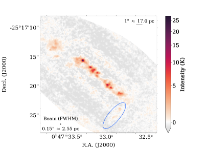
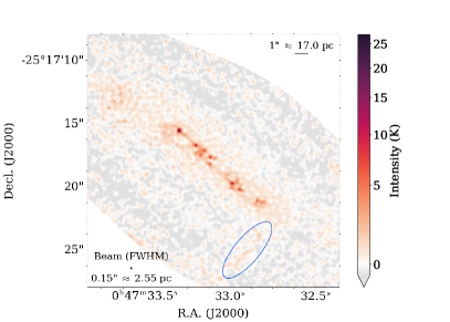
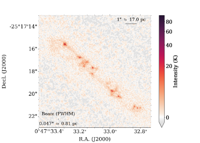
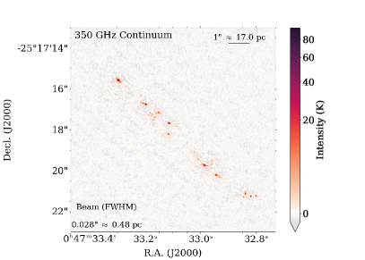
Figure 1: Top row: The 350 GHz 12-m+ACA dust continuum emission in the central 20″ (340 pc) of NGC 253, made by combining three 12-m configurations and one 7-m (ACA) configuration. The top left image shows the dirty map and the top right shows the cleaned map both convolved to a circular 0.15″ beam as described in Section 2.1.1. The blue ellipses highlight the SW streamer seen in the dust continuum emission (see Section 3). Bottom left: The 350 GHz continuum image in the central 10″ made by combining the three 12-m configurations, which has a final resolution of 0.047″. The cleaning has been optimized for the cluster-scales, as described in Section 2.1.2. Bottom right: The 350 GHz continuum image in the central 10″ of NGC 253 using only the highest resolution (0.028″) data from Levy et al. (2021).

Before cleaning the extended emission, it was necessary to carefully clean the point source-like clusters, otherwise the algorithm had a tendency to over-subtract these regions leaving deep negative bowls. We cleaned the emission from the clusters using scales=[0] and interactively controlled the threshold and number of iterations to avoid over-cleaning. We cleaned the point sources until they were no longer point-like in the residual map and so that the extended residual emission near the point sources was similar to the larger scale emission in the map.

Due to the range of spatial scales covered by these combined data sets, the algorithm tends to favor small scales, making cleaning the extended emission time consuming. Since, for the 12-m+ACA map, we are interested in the larger scale more diffuse emission, we used a $uv$-taper of 0.2″, scales=[0,8,16], smallscalebias=0 which gives equal weight to all scales to more efficiently clean the map. We used a circular 0.15″ restoring beam. To avoid over-cleaning, we reduced the gain of each major cycle to 0.05 and interactively lowered the threshold. We interactively cleaned the map until the residuals stopped changing. The final cleaned 12-m+ACA map is shown in Figure 1 (top right), which has an rms of 1.1 mJy beam^-1 (0.5 K) in regions away from emission.

2.1.2 Imaging the 12-m Data

We imaged the central 48″$\times$48″ of the line-flagged, channel averaged, combined 12-m visibilities interactively using tclean. Since we are interested in the dust continuum emission associated with the clusters, we use a different imaging strategy from the one described above. We use a cell (pixel) size of 0.0046″, the same as was used for the high resolution continuum map (Levy et al., 2021) which is shown for comparison in Figure 1 (bottom right). In all iterations, we used specmode=‘mfs’, deconvolver=‘multiscale’, Briggs weighting with robust=0.5, and apply the primary beam correction. The baseline was fit with a linear function (nterms=2) to account for any continuum slope over the bandpass.

As with the 12-m+ACA map, before cleaning the extended emission, it was necessary to carefully clean the point source-like clusters, otherwise the algorithm had a tendency to over-subtract these regions leaving deep negative bowls. We cleaned the emission from the clusters using scales=[0] and interactively controlled the threshold and number of iterations to avoid over-cleaning. We cleaned the point sources until they were no longer point-like and so that the emission in those regions was similar to the larger scale emission in the map.

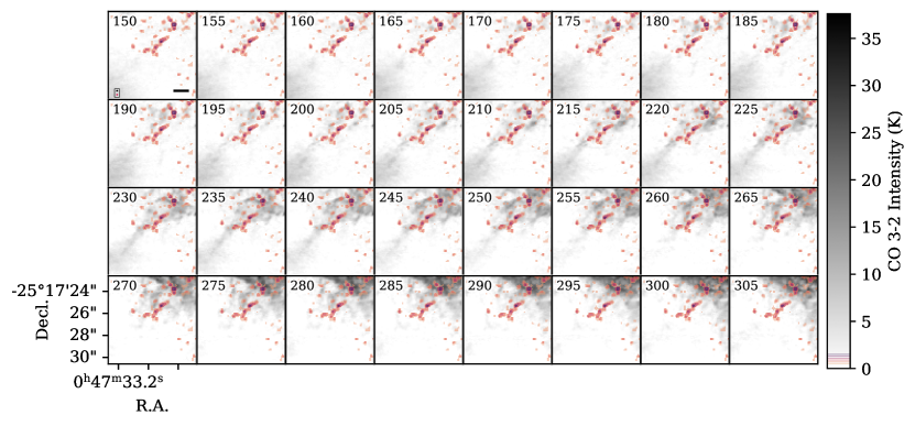
Figure 2: Channel maps of the CO $3-2$ emission showing the SW streamer (grayscale; Krieger et al., 2019). The LSRK velocity of each channel is shown in the upper left corner. The red/orange filled contours show the 350 GHz dust continuum emission from the 12-m+ACA data (top right panel of Figure 1). The contours span from $0.5-1.5$ K in steps of 0.2 K. We have removed data near the map edges where the signal is increased due to the primary beam correction. The FWHM beam sizes are shown in the box in the lower left corner of the first panel. Each panel is 135 pc (8″) on a side. The scale bar in the lower right corner of the first panel shows 20 pc. The 350 GHz continuum emission tends to trace the outer (southwest) edge of the SW streamer seen in CO.

Once the point sources were "cleaned", we carefully cleaned the more extended emission, starting from large scales and moving to smaller ones. For each iteration, we used smallscalebias=0 and no $uv$-taper. We first started with scales=[16,32,64] (corresponding to $\approx$0.07″, 0.15″, and 0.30″). We interactively cleaned these scales until the maximum residual and cleaned flux no longer changed significantly. We then added scales=[8] ($\approx$0.04″) to the existing scales and continued to clean interactively as before. After this scale was cleaned, the overall residuals resembled noise. The map had a FWHM Gaussian beam size of 0.045″$\times$0.041″. We convolved the image to a circular 0.0475″ beam. The final cleaned 12-m map is shown in Figure 1 (bottom left), which has an rms of 0.2 mJy beam^-1 (0.8 K) in regions away from emission.

3 South-West Streamer Detected in Dust Continuum Emission

In Figure 1 (top), we detect the SW streamer in 350 GHz dust continuum emission for the first time. The SW streamer is the brightest feature of the molecular outflow component and corresponds to the SW edge of the outflow cone. It was first detected in CO $1-0$ by Bolatto et al. (2013) and has subsequently been detected in other CO transitions and dense molecular gas tracers (e.g., Walter et al., 2017; Zschaechner et al., 2018; Krieger et al., 2019). High line ratios of HCN/CO in the SW streamer indicate that this component of the outflow originates from the central starburst (Walter et al., 2017). The SW streamer has an estimated age of $\sim 1$ Myr (Walter et al., 2017), in good agreement with the approximate ages of the massive star-forming regions in the starburst nucleus (see Section 5.4).

We compare the location of the dust component of the SW streamer to the CO $3-2$ from Krieger et al. (2019) in Figure 2. The CO $3-2$ data have a similar beam size (0.17″ $=2.88$ pc) as the dust map (0.15″ $=2.55$ pc; Figure 1, top right). The dust continuum emission has a similar morphology as the CO $3-2$, but is offset to the southwest. In the context of the larger-scale outflow, this means that the dust is found towards the outer edge of the outflow cone.

That the dust emission is primarily at the edge of the outflow cone may be an optical depth effect. We would expect the dust to be distributed as a hollow cone, like the outflowing molecular gas, which confines the hot outflowing material (e.g., Leroy et al., 2015b; Meier et al., 2015). In projection, the dust will have the highest optical depth along the line of sight in a streamer-like structure at the very edge of the projected outflow. This effect is illustrated in Figure 8 of Bolatto et al. (2021, see especially the purple regions of this figure). It is still unclear, however, precisely why there is such a large offset between the dust and CO $3-2$ in the SW streamer in NGC 253. While both CO and dust show temperature effects, the dust is more likely to remain a simple optically thin column density tracer and hence may better trace the true "spine" of the cone.

3.1 Inferred H₂ Column Density and Mass in the SW Streamer

We estimate the flux of dust emission in the SW streamer using the 12-m+ACA maps within the blue ellipse shown in Figure 1 (top right). The flux density in this region is $\approx 540\pm 180$ mJy. We convert this flux density to an estimated average H₂ column density and mass, assuming a dust-to-gas ratio of 1/100, a dust mass absorption coefficient of 1.9 cm² g^-1 following Leroy et al. (2018). We assume a dust temperature of 34 K (Gao & Solomon, 2004; Weiß et al., 2008; Mangum et al., 2013), but we note that the dust temperature is not well constrained in the outflow itself. We adopt a minimum dust temperature of 11 K (Zschaechner et al., 2018) and a maximum dust temperature of 50 K (Walter et al., 2017), which we propagate into our uncertainty on the column density and mass. This calculation yields N${}_{\rm H_{2}}\sim(4^{+6}_{-2})\times 10^{23}$ cm ^-1 and M${}_{\rm H_{2}}\sim(1.7^{+2.6}_{-0.8})\times 10^{7}$ M_⊙. The uncertainties are dominated by uncertainties on the dust temperature in the outflow. Since the outflow is expected to be warm (e.g., Leroy et al., 2015b; Walter et al., 2017; Zschaechner et al., 2018), the true column density and molecular gas mass are more likely to be N${}_{\rm H_{2}}\sim(2-4)\times 10^{23}$ cm ^-1 and M${}_{\rm H_{2}}\sim(8-17)\times 10^{6}$ M_⊙

Walter et al. (2017) estimated the H₂ column density in the SW streamer in two ways: from the CO $1-0$ and from the H$\alpha$/Pa$\beta$ line ratio. From the CO, they found N${}_{\rm H_{2}}\sim 4\times 10^{21}$ cm^-2, which is consistent with their extinction-based estimate of N${}_{\rm H_{2}}\sim 5\times 10^{21}$ cm^-2. They note, however, that the detection of bright emission from HCN and other molecules in the SW streamer implies a larger density of N${}_{\rm H_{2}}\sim 5\times 10^{22}$ cm^-2, in better agreement with our estimate. Our dust-based estimate of the H₂ mass in the SW streamer is consistent with the minimum mass of the SW streamer of $\sim 10^{6}$ M_⊙ found by Walter et al. (2017) and other CO-based measurements (i.e., Bolatto et al., 2013; Zschaechner et al., 2018; Krieger et al., 2019).

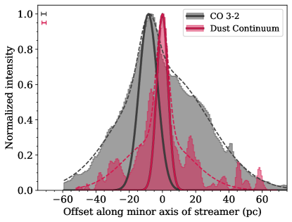
Figure 3: The normalized width profiles of the SW streamer, where the streamer has been summed along its major axis. The shaded histograms show the width profiles for the dust continuum (red) and CO $3-2$ (gray). For the CO, this profile is the integrated intensity over the velocity channels shown in Figure 4. These profiles are fit with a two-component Gaussian, shown as the dashed curves. The narrow components (corresponding to the outflow) of the fits are shown as the solid curves, where the respective beam sizes have been deconvolved. The FWHM beam sizes are shown in the upper left corner. The x-axis is the offset along the minor axis of the streamers relative to the centroid of the narrow dust component. The dust continuum component of SW streamer is intrinsically narrower than and offset from the CO $3-2$.

3.2 Width of the SW Streamer in Dust and CO $3-2$

We estimate the width of the dust emission in the SW streamer, summing the emission along the major axis of the streamer (PA $\approx 140$^∘). This yields a profile of the summed intensity along the minor axis of the SW streamer (red histogram in Figure 3). We fit a two component Gaussian to this width profile, with one narrow component for the streamer and a broad component for any disk emission. We remove the beam in quadrature from the width of the narrow component and show this beam-deconvolved narrow component corresponding to the outflow in Figure 3. The dust streamer has a beam-deconvolved FWHM of 8 pc.

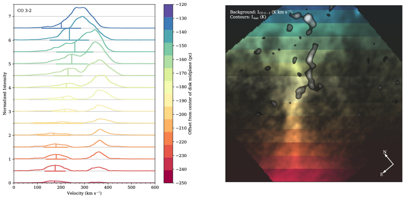
Figure 4: Left: CO $3-2$ spectra in slices along the SW streamer. The CO $3-2$ data are binned in 10 pc bins along the major axis of the outflow, as indicated by the colorbar. The data are summed in each bin and normalized based on the maximum intensity. The spectra are offset artificially along the y-axis. The velocity component corresponding to the outflow is fit with a Gaussian, where the mean and FWHM velocity are indicated by the vertical and horizontal line segments. Right: The SW streamer seen in CO $3-2$ (colored background) and the 350 GHz dust emission (grayscale contours), rotated so the major axis is vertical and the top of the image is closest to the midplane. For the CO $3-2$, data in each 10 pc bin is color coded based on its offset from the midplane according to the colorbar in the left panel. We find the integrated intensity over the channels within one FWHM from the central velocity (i.e., over velocities indicated by the horizontal line segments in the left panel). The dust continuum contours are the same as in Figure 2.

We compare the width of the dust streamer to that of the CO $3-2$. First, we kinematically identify the components of the CO $3-2$ emission associated with the SW streamer, using a method similar to that of Walter et al. (2017) for the CO $1-0$ (see their Section 3.2). We take position-velocity slices through the CO data cube over the field-of-view (FOV) shown in Figure 2. Each slice is 10 pc wide along the major axis of the SW streamer. Pixels within each slice are summed to produce the spectra shown in Figure 4 (left). Away from the midplane, the CO $3-2$ has two velocity components, where the blueshifted component traces the outflow and the redshifted component primarily traces emission from the central starburst and disk. We fit the outflow component with a Gaussian at each offset, where the mean velocity and FWHM are indicated by the vertical and horizontal lines for each spectrum in Figure 4 (left). Using these fits, we calculate the integrated CO $3-2$ intensity over the FWHM velocity range of the outflow component for each slice. This integrated intensity map is shown in Figure 4 (right) where the color coding of the image indicates the offset from the midplane as in the left panel. We overplot contours of the dust continuum emission to again highlight the offset between the dust and CO in the SW streamer. We measure the width of the CO $3-2$ SW streamer using this integrated intensity map following the same procedure as for the dust described in the previous paragraph. We note that the beam sizes of the 350 GHz continuum and CO $3-2$ are very similar (2.55 pc and 2.88 pc respectively). The width profile and Gaussian fits for the CO $3-2$ are shown in Figure 3 (gray). The beam-deconvolved FWHM of the CO $3-2$ associated with the SW streamer is 13 pc. The SW streamer seen in the dust continuum is narrower than in the CO by a factor of $\sim 1.6$. The peak of the dust continuum is offset to the southwest of the peak of the CO $3-2$ by 8 pc ($\sim 3\times$ the FWHM beam size).

4 Cluster Size, Flux, and Mass Measurements

Accurate sizes and masses for the SSCs are crucial to understand their physical properties and compare to numerical simulations (e.g., Grudić et al., 2021). Previous studies which have measured these parameters used data which marginally resolved the SSCs (e.g., Leroy et al., 2018; Rico-Villas et al., 2020; Mills et al., 2021). However, using 0.5 pc resolution data, Levy et al. (2021) showed that the SSCs seen in the 350 GHz dust continuum emission break apart into multiple components once they are spatially resolved. Those data, however, used only the most extended ALMA configurations and hence lacked the short spacings which are sensitive to extended emission. This short spacing information is important to accurately measure the flux of the clusters as well as the background of extended emission in which they are embedded. Accurate measurements of the SSC sizes and masses, therefore, require both high spatial resolution and complete sampling of the Fourier plane.

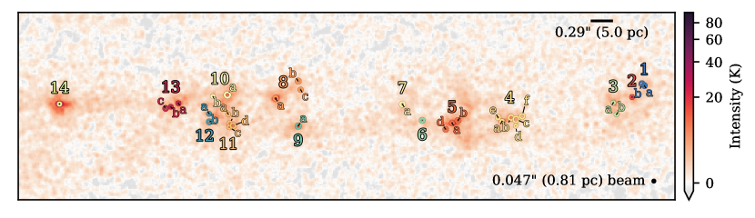
Figure 5: The continuum sizes of the SSCs over the high resolution combined 350 GHz continuum map. The map has been rotated counterclockwise by 42^∘ so that the SSC structure is horizontal. The colored circles show the deconvolved radii from the Gaussian fits to the radial profiles (Table 1). The cluster groups are labeled and colored following the nomenclature of Leroy et al. (2018). Clusters that break apart in the higher resolution images are denoted with letters in order of decreasing brightness.

As described in Section 2, in this work we combine three configurations of 12-m data from ALMA. These data have a resolution of 0.8 pc, which allows us to spatially resolve the SSCs, and a maximum recoverable scale of 66 pc, allowing us to measure the flux of the SSCs and background emission. We, therefore, re-measure the cluster positions and sizes using the 0.8 pc resolution map (Figure 1 bottom left) as described below.

4.1 Identifying the Continuum Sources

Table 1: Deconvolved SSC Parameters

SSC #	R.A.	Decl.	$I_{\mathrm{peak}}$	$r_{\mathrm{deconv}}$	Flux	log10Mgas
	(J2000)	(J2000)	(K)	(pc)	(mJy)	(log10M⊙)
1a	$0^{\mathrm{h}}47^{\mathrm{m}}32.801^{\mathrm{s}}$	$-25^{\circ}17{}^{\prime}21.242{}^{\prime\prime}$	$6.4\pm 0.4$	$0.58\pm 0.04$	$2.1\pm 0.1$	$4.3\pm 0.1$
1b	$0^{\mathrm{h}}47^{\mathrm{m}}32.801^{\mathrm{s}}$	$-25^{\circ}17{}^{\prime}21.197{}^{\prime\prime}$	$5.0\pm 2.6$	$0.60\pm 0.18$	$1.8\pm 0.9$	$4.2\pm 0.3$
2	$0^{\mathrm{h}}47^{\mathrm{m}}32.819^{\mathrm{s}}$	$-25^{\circ}17{}^{\prime}21.248{}^{\prime\prime}$	$23.3\pm 1.6$	$0.44\pm 0.02$	$4.4\pm 0.3$	$4.6\pm 0.1$
3a	$0^{\mathrm{h}}47^{\mathrm{m}}32.839^{\mathrm{s}}$	$-25^{\circ}17{}^{\prime}21.122{}^{\prime\prime}$	$22.5\pm 1.9$	$0.43\pm 0.03$	$4.0\pm 0.3$	$4.6\pm 0.1$
3b	$0^{\mathrm{h}}47^{\mathrm{m}}32.845^{\mathrm{s}}$	$-25^{\circ}17{}^{\prime}21.285{}^{\prime\prime}$	$7.1\pm 0.9$	$0.43\pm 0.04$	$1.3\pm 0.2$	$4.1\pm 0.1$
4a	$0^{\mathrm{h}}47^{\mathrm{m}}32.945^{\mathrm{s}}$	$-25^{\circ}17{}^{\prime}20.212{}^{\prime\prime}$	$27.2\pm 1.9$	$0.48\pm 0.03$	$6.0\pm 0.4$	$4.8\pm 0.1$
4b	$0^{\mathrm{h}}47^{\mathrm{m}}32.934^{\mathrm{s}}$	$-25^{\circ}17{}^{\prime}20.259{}^{\prime\prime}$	$7.5\pm 0.4$	$0.63\pm 0.05$	$2.9\pm 0.2$	$4.4\pm 0.1$
4c	$0^{\mathrm{h}}47^{\mathrm{m}}32.932^{\mathrm{s}}$	$-25^{\circ}17{}^{\prime}20.327{}^{\prime\prime}$	$5.1\pm 0.4$	$0.74\pm 0.10$	$2.7\pm 0.2$	$4.4\pm 0.1$
4d	$0^{\mathrm{h}}47^{\mathrm{m}}32.937^{\mathrm{s}}$	$-25^{\circ}17{}^{\prime}20.398{}^{\prime\prime}$	$4.1\pm 4.3$	$0.38\pm 0.16$	$0.6\pm 0.6$	$3.7\pm 0.5$
4e	$0^{\mathrm{h}}47^{\mathrm{m}}32.945^{\mathrm{s}}$	$-25^{\circ}17{}^{\prime}20.126{}^{\prime\prime}$	$4.7\pm 0.6$	$0.54\pm 0.09$	$1.3\pm 0.2$	$4.1\pm 0.1$
4f	$0^{\mathrm{h}}47^{\mathrm{m}}32.924^{\mathrm{s}}$	$-25^{\circ}17{}^{\prime}20.354{}^{\prime\prime}$	$3.7\pm 0.3$	$0.62\pm 0.09$	$1.4\pm 0.1$	$4.1\pm 0.1$
5a	$0^{\mathrm{h}}47^{\mathrm{m}}32.987^{\mathrm{s}}$	$-25^{\circ}17{}^{\prime}19.727{}^{\prime\prime}$	$49.4\pm 3.5$	$0.47\pm 0.03$	$10.5\pm 0.7$	$5.0\pm 0.1$
5b	$0^{\mathrm{h}}47^{\mathrm{m}}32.980^{\mathrm{s}}$	$-25^{\circ}17{}^{\prime}19.756{}^{\prime\prime}$	$10.5\pm 8.5$	$0.59\pm 0.47$	$3.6\pm 3.7$	$4.5\pm 0.6$
5d	$0^{\mathrm{h}}47^{\mathrm{m}}32.997^{\mathrm{s}}$	$-25^{\circ}17{}^{\prime}19.734{}^{\prime\prime}$	$5.1\pm 0.7$	$0.57\pm 0.10$	$1.6\pm 0.2$	$4.1\pm 0.1$
6	$0^{\mathrm{h}}47^{\mathrm{m}}33.010^{\mathrm{s}}$	$-25^{\circ}17{}^{\prime}19.395{}^{\prime\prime}$	$3.4\pm 0.5$	$0.58\pm 0.10$	$1.1\pm 0.2$	$3.6\pm 0.1$
7a	$0^{\mathrm{h}}47^{\mathrm{m}}33.014^{\mathrm{s}}$	$-25^{\circ}17{}^{\prime}19.015{}^{\prime\prime}$	$3.0\pm 0.2$	$0.59\pm 0.06$	$1.0\pm 0.1$	$4.0\pm 0.1$
8a	$0^{\mathrm{h}}47^{\mathrm{m}}33.114^{\mathrm{s}}$	$-25^{\circ}17{}^{\prime}17.675{}^{\prime\prime}$	$27.7\pm 1.8$	$0.57\pm 0.04$	$8.7\pm 0.6$	$4.9\pm 0.1$
8b	$0^{\mathrm{h}}47^{\mathrm{m}}33.083^{\mathrm{s}}$	$-25^{\circ}17{}^{\prime}17.707{}^{\prime\prime}$	$3.9\pm 0.3$	$0.61\pm 0.07$	$1.4\pm 0.1$	$4.1\pm 0.1$
8c	$0^{\mathrm{h}}47^{\mathrm{m}}33.087^{\mathrm{s}}$	$-25^{\circ}17{}^{\prime}17.828{}^{\prime\prime}$	$2.8\pm 0.4$	$0.51\pm 0.09$	$0.7\pm 0.1$	$3.8\pm 0.1$
9a	$0^{\mathrm{h}}47^{\mathrm{m}}33.116^{\mathrm{s}}$	$-25^{\circ}17{}^{\prime}18.211{}^{\prime\prime}$	$13.0\pm 0.5$	$0.61\pm 0.03$	$4.7\pm 0.2$	$4.5\pm 0.1$
10a	$0^{\mathrm{h}}47^{\mathrm{m}}33.151^{\mathrm{s}}$	$-25^{\circ}17{}^{\prime}17.149{}^{\prime\prime}$	$9.1\pm 0.8$	$0.71\pm 0.07$	$4.4\pm 0.4$	$4.6\pm 0.1$
10b	$0^{\mathrm{h}}47^{\mathrm{m}}33.164^{\mathrm{s}}$	$-25^{\circ}17{}^{\prime}17.018{}^{\prime\prime}$	$5.3\pm 2.4$	$0.35\pm 0.10$	$0.6\pm 0.3$	$3.7\pm 0.3$
11a	$0^{\mathrm{h}}47^{\mathrm{m}}33.165^{\mathrm{s}}$	$-25^{\circ}17{}^{\prime}17.376{}^{\prime\prime}$	$13.1\pm 1.7$	$0.39\pm 0.03$	$1.9\pm 0.2$	$4.0\pm 0.1$
11b	$0^{\mathrm{h}}47^{\mathrm{m}}33.170^{\mathrm{s}}$	$-25^{\circ}17{}^{\prime}17.491{}^{\prime\prime}$	$9.0\pm 1.2$	$0.50\pm 0.06$	$2.2\pm 0.3$	$4.1\pm 0.1$
11c	$0^{\mathrm{h}}47^{\mathrm{m}}33.174^{\mathrm{s}}$	$-25^{\circ}17{}^{\prime}17.530{}^{\prime\prime}$	$8.5\pm 4.0$	$0.48\pm 0.22$	$1.9\pm 1.0$	$4.0\pm 0.3$
11d	$0^{\mathrm{h}}47^{\mathrm{m}}33.170^{\mathrm{s}}$	$-25^{\circ}17{}^{\prime}17.550{}^{\prime\prime}$	$7.9\pm 0.6$	$0.68\pm 0.06$	$3.5\pm 0.3$	$4.3\pm 0.1$
12a	$0^{\mathrm{h}}47^{\mathrm{m}}33.180^{\mathrm{s}}$	$-25^{\circ}17{}^{\prime}17.177{}^{\prime\prime}$	$5.4\pm 0.5$	$0.48\pm 0.05$	$1.2\pm 0.1$	$3.5\pm 0.1$
12b	$0^{\mathrm{h}}47^{\mathrm{m}}33.186^{\mathrm{s}}$	$-25^{\circ}17{}^{\prime}17.268{}^{\prime\prime}$	$3.4\pm 0.5$	$0.59\pm 0.14$	$1.1\pm 0.2$	$3.5\pm 0.2$
13a	$0^{\mathrm{h}}47^{\mathrm{m}}33.198^{\mathrm{s}}$	$-25^{\circ}17{}^{\prime}16.750{}^{\prime\prime}$	$52.0\pm 3.6$	$0.44\pm 0.03$	$9.5\pm 0.7$	$5.0\pm 0.1$
13b	$0^{\mathrm{h}}47^{\mathrm{m}}33.207^{\mathrm{s}}$	$-25^{\circ}17{}^{\prime}16.712{}^{\prime\prime}$	$11.8\pm 0.8$	$0.47\pm 0.04$	$2.5\pm 0.2$	$4.4\pm 0.1$
13c	$0^{\mathrm{h}}47^{\mathrm{m}}33.212^{\mathrm{s}}$	$-25^{\circ}17{}^{\prime}16.678{}^{\prime\prime}$	$4.8\pm 1.4$	$0.57\pm 0.17$	$1.5\pm 0.5$	$4.2\pm 0.2$
14	$0^{\mathrm{h}}47^{\mathrm{m}}33.297^{\mathrm{s}}$	$-25^{\circ}17{}^{\prime}15.560{}^{\prime\prime}$	$90.3\pm 6.7$	$0.45\pm 0.03$	$17.6\pm 1.3$	$5.3\pm 0.1$

Note. — See Section 4 for details.

From the 0.48 pc resolution continuum data, many of the candidate SSCs identified by Leroy et al. (2018) at 2 pc resolution break apart into smaller structures (Figure 1 bottom right; Levy et al. 2021). We find more than three dozen dust clumps by-eye in the 0.48 pc resolution dust image. The SSCs identified by Leroy et al. (2018) remain the largest and brightest structures. We, therefore, follow the SSC nomenclature of Leroy et al. (2018), but add letters to sources that break apart in order of decreasing brightness, as described by Levy et al. (2021). From there, we match the locations of the dust clumps from the 0.48 pc resolution image to the 0.81 pc resolution map (Figure 1 bottom left). The 0.81 pc resolution map combines three configurations of ALMA data and, therefore, better recovers the extended emission than the 0.48 pc resolution map. From the 0.81 pc map, we identify 33 clumps of dust emission, which are listed in Table 1 and are shown in Figure 5. Some of the very small sources previously identified in the 0.48 pc resolution image are no longer visible in the 0.81 pc resolution image due to the slightly lower resolution and extended emission (i.e., SSCs 1c, 3c, 5c, 7b, 9b). For SSCs 7a and 9a, we retain the "a" lettering to indicate that these clusters do break apart in the 0.48 pc resolution image, though these smaller clusters are not visible in the 0.i81 pc resolution map. Clusters without letters (SSCs 2, 6, 14) do not break apart even in the 0.48 pc resolution dust continuum map.

4.2 Cluster Positions

To measure the precise centers of the SSCs, we fit the continuum intensity map with a 2D rotated elliptical Gaussian function. We include a constant background component since the clusters are embedded within more extended emission. Before fitting, we mask out other sources in the images. This is especially important for clusters in crowded fields. We automatically mask out primary clusters based on their half-flux radii ($r_{\rm half-flux}$) measured from the high resolution data (Levy et al., 2021), removing pixels within 2$\times r_{\rm half-flux}$ from the cluster centers. We remove contaminating subclusters by-eye and remove pixels within 1.5$\times$ the beam half-width-half-maximum (HWHM) from the cluster centers.

For some of the weaker clusters, the 2D elliptical Gaussian fit does not converge. In these cases, we determine the center position based on the brightest pixel in the dust continuum near the center of the SSC. The best-fitting SSC centers are listed in Table 1 and shown in Figure 5. We estimate that the positional accuracy of this image is $\approx 2.5$ milliarcseconds (0.04 pc).

4.3 Radial Profiles

We construct radial profiles for each cluster. Before extracting the radial profiles, we mask the images in the same way as for the 2D Gaussian fitting. We use concentric circular annuli centered on the R.A. and Decl. from the 2D Gaussian fitting (Table 1). The width of the annuli is the beam HWHM (0.024″ = 0.40 pc) and the last ring has a radius of 3$\times$ the beam FWHM ($3\times 0.0475$″ = 2.4 pc). We measure the median intensity in each annulus, which is shown in Figure 6 for SSC 14; the uncertainty is the standard error in each annulus.

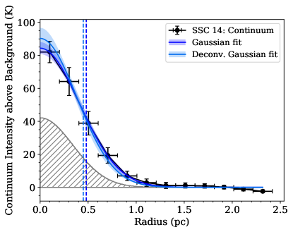
Figure 6: The extracted radial profile of SSC 14 (black data points). The gray hatched region shows the Gaussian beam with arbitrary vertical scaling. The dark blue curve shows the Gaussian fit to the radial profile. The dark blue shaded region around this curve reflects the standard deviation of 500 Monte Carlo realizations varying the data points within the errorbars. The vertical dark blue dashed line shows the HWHM radius. The light blue curve shows the beam-deconvolved (i.e., intrinsic) Gaussian radial profile, where the shaded region shows the propagated uncertainties on the fit and the vertical light blue dashed line shows the deconvolved HWHM radius.

We model the cluster radial profiles using a Gaussian of the form

$${\rm SB}(r)=ae^{-\frac{r^{2}}{2\sigma^{2}}}+c$$ (1)

to model the radial surface brightness (SB) profile of the clusters. We also include a constant background component ($c$) since the clusters sit in an extended background of dust emission. An example of this model fit to the cluster radial profile is shown for SSC 14 in Figure 6, where the fitted background level ($c$) has been removed. We determine the uncertainty on the Gaussian fit using a Monte Carlo simulation where we randomly vary the data points within the errorbars. The dark blue shaded region in Figure 6 reflects the standard deviation of 500 trials.

In addition to a Gaussian function, we also modeled the radial profiles using King (1962) and Plummer (1911) profiles. These provide equally good fits to the cluster radial profiles. We proceed using the Gaussian fits to the radial profiles.

4.4 Deconvolved Sizes, Fluxes, and Gas Masses

We deconvolve the beam size from the fitted Gaussian profile by removing the (Gaussian) beam HWHM in quadrature. We produce deconvolved Gaussian radial profiles using the deconvolved radii and conserving the flux. An example of the deconvolved Gaussian radial profile is shown for SSC 14 in Figure 6. We report the deconvolved cluster radii (r_deconv), peak intensities ($I_{\rm peak}$), and fluxes in Table 1. For $I_{\rm peak}$, we subtract the background level so this value reflects the peak intensity of the cluster above the background of surrounding material. We show the distribution of intrinsic cluster radii in Figure 7. Our intrinsic radii cover a narrow range of radii from $\approx 0.25-0.70$ pc. We also show the deconvolved radii for each of the clusters in Figure 5 over the continuum image.

We compare our measured cluster radii to those measured by Brown & Gnedin (2021) from the Legacy Extragalactic UV Survey (LEGUS) survey (Calzetti et al., 2015). These clusters are identified in 31 nearby galaxies in five bands from the near-UV to near-IR. Brown & Gnedin (2021) measure the intrinsic stellar half-light (effective) radii of the young star clusters in these galaxies from the "white light" (i.e. combined 5-filter) images. From their cluster catalog, we select clusters with reliable radius and mass measurements, ages $\leq 2$ Myr, and stellar masses $\geq 10^{4}$ M_⊙; see Brown & Gnedin (2021) for the definitions of these quantities. We show a kernel density estimator (KDE) of the LEGUS cluster radii in gray in Figure 7, where the inset shows the KDE over their full radius range. The LEGUS clusters tend to be larger than the SSCs studied here. The peak in the LEGUS radius distribution for clusters with the above selection criteria is between $2-3$ pc.

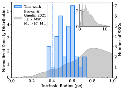
Figure 7: The light blue histogram shows the distribution of the intrinsic SSC radii, measured from the beam-deconvolved Gaussian fit to the radial profile. The left y-axis shows the histogram normalized to unit area, whereas the right y-axis shows the number of SSCs in each bin. The vertical blue dashed line shows the beam HWHM. The gray KDE shows the distribution of star cluster intrinsic effective radii measured in LEGUS galaxies normalized to unit area over the plotted radius range (Brown & Gnedin, 2021). We select clusters with ages $<2$ Myr and stellar masses $>10^{4}$ M_⊙ to be most comparable to our sample of very young, massive clusters. The inset in the upper right shows the full distribution of the LEGUS radii with the same selection criteria, which peaks around radii of $2-3$ pc. The vertical black line marks 1 pc, the radial extent shown in the main panel.

It is perhaps not unexpected that the clusters identified by Brown & Gnedin (2021) are larger. The radii we measure for the clusters in NGC 253 correspond to the size of the dust (and molecular gas) envelopes, whereas the radii measured for the LEGUS clusters come from the stellar light. The clusters in NGC 253 are still in the process of forming (Leroy et al., 2018; Rico-Villas et al., 2020; Mills et al., 2021) and are, therefore, still very compact. Since the LEGUS clusters are typically older than most of the SSCs in this work and are no longer (deeply) embedded in their natal molecular clouds, it is possible that the stellar light would extend to larger radii than the compact dust emission from the SSCs. Simulations of star cluster evolution show an increase in the radius with age due primarily to mass loss from stellar winds of young massive stars (e.g., Portegies Zwart et al., 2010, and references therein).

We estimate the gas masses of the clusters based on their 350 GHz dust continuum emission, following Leroy et al. (2018, see their Section 4.3.3 for more details). Assuming a fiducial dust temperature of $T_{\rm dust}=130$ K, we convert the deconvolved peak intensity at 350 GHz to a dust optical depth via

$$\tau_{\rm 350~{}GHz}=-\ln\left[1-\frac{I_{\rm 350~{}GHz}}{B_{\nu}(T_{\rm dust})}\right]$$ (2)

where $I_{\rm 350~{}GHz}$ is the peak intensity in Table 1 and $B_{\nu}(T_{\rm dust})$ is the Planck function evaluated at 350 GHz for our adopted value of $T_{\rm dust}$. Though we do not yet have measurements of the dust temperatures towards these SSCs, the peak intensities of $\gtrsim 25$ K we measure towards some of these clusters (Table 1) supports a high value of $T_{\rm dust}$. We convert the dust optical depth to a gas surface mass density where

$$\Sigma_{\rm gas}=\frac{\tau_{\rm 350~{}GHz}}{\rm DGR\ \kappa_{\rm 350~{}GHz}}$$ (3)

where the dust-to-gas ratio (DGR) is assumed to be 1/100. The central 300 pc of NGC 253 is known to have a somewhat super-solar gas-phase metallicity ($Z=2.2Z_{\odot}$; Galliano et al. 2008; Davis et al. 2013). $\kappa_{\rm 350~{}GHz}$ is the mass absorption coefficient; we assume a value of 1.9 cm² g^-1, but this value is uncertain by a factor of $\sim$2 (Ossenkopf & Henning, 1994; Leroy et al., 2018). Finally, we convert the gas mass surface density to a gas mass by multiplying by the area of the cluster:

$${\rm M}_{\rm gas}=\Sigma_{\rm gas}{\rm A}_{\rm deconv}$$ (4)

where

$${\rm A}_{\rm deconv}\equiv\frac{4\pi{\rm r}_{\rm deconv}^{2}}{2\ln 2}$$ (5)

is the area of a 2D Gaussian whose HWHM is equal to the beam-deconvolved radius measurement ($r_{\rm deconv}$; Table see 1).

4.5 Flux Density and Gas Mass Distributions

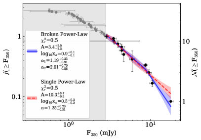
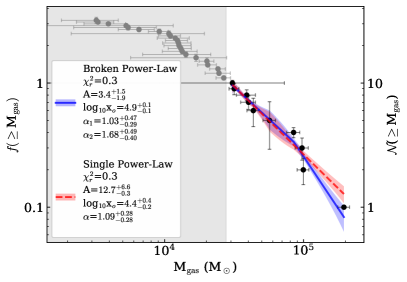
Figure 8: The cluster flux density (left) and molecular gas mass (right) functions. The right y-axis shows the number of clusters whereas the left y-axis shows the fraction of clusters with reliable measurements. The gray shaded regions and gray points show our estimate of confusion; measurements in this region are likely underestimated beyond the uncertainties. We fit the distributions with a broken power law (blue solid lines) and a single power law (red dashed lines). See Section 4.5 for details on the uncertainty calculations and the fitting.

From the fluxes (Table 1), we construct the cluster flux density function, which is shown in Figure 8 (left). This is essentially a cumulative distribution function (CDF), where the ordinate counts the number of clusters with flux densities larger than the value on the abscissa. The horizontal error bars come from the uncertainties on the measured fluxes. To determine the vertical error bars, we use a Monte Carlo calculation, allowing the measured fluxes to vary uniformly within their uncertainties. This can change the ordering of the flux densities and hence the CDF. We perform 100 trials of the Monte Carlo, and report the standard deviation of the CDF for each point over those trials as the vertical error bars. We repeat this procedure with the gas masses which are shown in Figure 8 (right).

Both distributions appear to follow a broken power law, with a break at the very low flux/mass end; however, this break is very likely due to incompleteness at the low flux end of the distribution (e.g., Emig et al., 2020). The SSC identification is done by-eye based on the 0.5 pc resolution continuum image (Figure 1 bottom right). The radial profiles are measured from the 0.8 pc resolution image (Figure 1 bottom left) at the locations of the SSCs identified from the high resolution image, as long as they are still apparent in the lower resolution image. The major uncertainty matching the SSCs between these images are from the "speckles" seen in the 0.8 pc resolution continuum image (Figure 1 bottom left). These speckles arise in the imaging by modeling the extended emission as Gaussians matched to the beam size, and they can resemble small, compact clusters. We, therefore, use these speckles as our test particles to evaluate the completeness and confusion of our SSC flux and gas mass functions. We choose a speckle in the image and measure its radial profile, beam-deconvolved size, and peak intensity as described in Sections 4.3 and 4.4. We find that a typical speckle has a flux of $\approx 3.5$ mJy and hence an inferred gas mass of $\approx 5\times 10^{4.5}$ M_⊙. We show these values as the gray shaded regions in Figure 8. Clusters with fluxes or masses near or below this limit are likely more uncertain than represented by the error bars, and we may be missing SSCs in this flux and mass regime.

For values above our completeness threshold, we fit the cluster flux density and gas mass functions using a broken power law of the form

$$f(x)=\begin{cases}A\left(\frac{x}{x_{0}}\right)^{-\alpha_{1}}\text{; $x<x_{0}$,}\\ A\left(\frac{x}{x_{0}}\right)^{-\alpha_{2}}\text{; $x>x_{0}$,}\end{cases}$$ (6)

which is implemented using BrokenPowerLaw1D from Astropy. As a comparison, we also fit the cluster flux density function with a single power law of the form

$$f(x)=A\left(\frac{x}{x_{0}}\right)^{-\alpha}$$ (7)

which is implemented using PowerLaw1D from Astropy.

We obtain the uncertainties on the fitted parameters using the same Monte Carlo approach described above. As the flux density or mass points are allowed to vary within their uncertainties, we re-fit Equation 6 at each iteration. The uncertainties listed in Figure 8 reflect the 16^th and 84^th percentiles (i.e., the inner 68%) of the parameter distributions after the Monte Carlo. The same strategy is used to obtain the uncertainties on the model curves, shown as the colored shaded regions in Figure 8.

When the completeness is accounted for, both the broken and single power law fits are able to reproduce the flux and gas mass distributions equally well ($\chi_{r}^{2}=0.3-0.5$; Figure 8). We find a single power law slope of 1.25 (1.09) for the flux (gas mass) functions. When we fit a broken power law, we measure a slope of 2.01 (1.58) at the high flux (gas mass) end.

Previous literature studies typically investigate the cluster stellar mass function. Recently, Mok et al. (2019, 2020) studied the cluster stellar mass function of a sample of star-forming galaxies. The young clusters included in their studies are older on average and span a wider range of stellar masses than the SSCs in NGC 253 (Leroy et al., 2018; Mills et al., 2021). Mok et al. (2019) found no evidence of a high-mass cut-off of the cluster stellar mass functions though other studies have found evidence of a high-mass cut off (e.g., Gieles et al., 2006; Whitmore et al., 2010; Adamo et al., 2015, 2017; Hollyhead et al., 2016; Johnson et al., 2017; Messa et al., 2018a, b).

Although our measurements are of the gas mass (not the stellar mass), we also do not see strong evidence for a high-mass cut-off up to $2\times 10^{5}$ M_⊙, which would be indicated by a more apparent break in the gas mass distribution (Figure 8 right). While our two highest mass clusters may hint at a break around $10^{4.9}$ M_⊙, statistically the single and broken power law fits are equally good (as indicated by $\chi_{r}^{2}$). This break (or truncation) mass is similar to what has been measured in other nearby galaxies (see e.g., discussion and references in Messa et al., 2018a).

Mok et al. (2020) found that the mass functions are well fit by single power laws (Equation 7) with slopes $2.0\pm 0.3$, in agreement with previous theoretical and observational studies (e.g., Zhang & Fall, 1999; Fall & Chandar, 2012; Chandar et al., 2017; Krumholz et al., 2019). When the clusters are fit in age bins, the youngest clusters have somewhat shallower power law slopes, with an average of $1.7\pm 0.5$, though this is still consistent with the full sample within the uncertainties (Mok et al., 2019). Messa et al. (2018a) studied the cluster mass function in M51. Although they preferred a Schechter function, they performed single power law fits as well. From their fits using a minimum mass of $10^{4}$ M_⊙ (similar to our completeness limit), Messa et al. (2018a) found a single power law slope of $2.67\pm 0.03$, steeper than found by Mok et al. (2020). The power law slope is reduced to $2$ (within the uncertainties) if the power law is truncated and if the minimum mass is reduced (see their Table 8).

The average slopes for the youngest clusters found by both Mok et al. (2020) and Messa et al. (2018a) are steeper than, but close to, the slope we measure for the gas mass distribution in NGC 253. We caution, however, that we are measuring the gas mass whereas Mok et al. (2019, 2020) and Messa et al. (2018a) measured the stellar mass of the clusters. Both Leroy et al. (2018) and Mills et al. (2021) found a median M_gas/M${}_{*}\approx 1$ for the clusters, but with appreciable scatter (average $\approx 2$, standard deviation $\approx 2.5$) using different tracers of the stellar and gas masses. This scatter from cluster to cluster means that the slope of the stellar function function in NGC 253 may be different than measured for the gas mass.

5 The Morpho-Kinematic Architecture of the SSCs

The quasi-linear arrangement of the SSCs in the center of NGC 253 is striking (e.g., Figures 1 and 5). In projection, this structure measures $\sim 155{\rm~{}pc}\times 15{\rm~{}pc}$ in diameter with a major axis position angle (PA) of $\approx 48^{\circ}$ east-of-north. This axis ratio of $\sim 10$ may suggest that the structure is intrinsically very thin and/or that we are seeing this structure at a high inclination. The galactic disk of NGC 253 is nearly edge-on, with an inclination of $\approx 78^{\circ}$ and a PA of $\approx 50^{\circ}$ (e.g., Pence, 1980; Westmoquette et al., 2011; Krieger et al., 2019). On $\sim$ kpc scales, the bar also has an inclination of $\approx 78^{\circ}$ but has a major-axis PA of $68^{\circ}$ (Scoville et al., 1985; Sorai et al., 2000). The quasi-linear arrangement of SSCs has approximately the same PA as the galaxy disk and is offset from the PA of the bar.

Using CO observations at 35 pc resolution, Leroy et al. (2015a) measure the geometry of the GMC structures in which these SSCs are embedded. They build 3D models of the GMC geometry as a disk, a linear bar-like arrangement, and a hybrid model. They find that the hybrid model provides the best fit to the data, where the inner $\sim 100-150$ pc (diameter) is more disk-like and regions beyond this extending out to $\sim 850-1400$ pc (diameter) have a more linear structure. They find that the maximum vertical thickness of the GMC structure is $<100$ pc for the molecular gas traced by CO and $<55$ pc for the denser molecular gas. Our measurement of the minor axis width of the SSC structure sets a maximum vertical extent of $<15$ pc, similar to the vertical extent of the MW CMZ (e.g., Molinari et al., 2011; Kruijssen et al., 2015; Shin et al., 2017; Henshaw et al., 2022).

Figure 9: NGC 253 as seen in the $J$-band from 2MASS (grayscale). The images on the left are 16 kpc (15.7′) on a side; the images on the right are 3 kpc (2.9′) on a side. The gray squares mark the inner 280 pc, the FOV of the ALMA data. In the right column, the gray $\times$ shows the kinematic center determined by Anantharamaiah & Goss (1996). Top row: Overplotted are the locations of important resonances and features, determined by Sorai et al. (2000). Working inward, the solid ellipses show the CR (green), the OILR (dark blue), and the IILR (light blue). We note that the location of the IILR is highly uncertain (see the discussion in Section 5.1). The gray circles in the lower right corners show the 16″ ($\sim$270 pc) beam of the CO $1-0$ observations used by Sorai et al. (2000). Bottom row: The outermost and innermost $x_{1}$ orbits are shown in red, and the outermost and innermost $x_{2}$ orbits are shown in pink (Das et al., 2001).

5.1 Bar Resonances and Families of Orbits in NGC 253

5.1.1 Bar Resonances

Zooming out in scale, Sorai et al. (2000) used CO $1-0$ data with 16″ ($\sim$270 pc) resolution from the Nobeyama 45-m telescope to study the bar resonances and kinematics in the center of NGC 253. By fitting the CO rotation curve, they were able to estimate the locations of several key bar resonances. From their CO rotation curve, they measure the angular velocity, $\Omega(R)$, and the epicyclic frequency, $\kappa(R)$. We note that Sorai et al. (2000) used an older distance for NGC 253 of 2.5 Mpc; here we have converted all of their measurements assuming a galaxy distance of 3.5 Mpc1. Sorai et al. (2000) used previous estimates of the pattern speed of the bar, $\Omega_{p}\approx 35$ km s^-1 kpc^-1. The radius at which $\Omega_{p}=\Omega$ is called the corotation radius (CR) and occurs at a radius of 5.6 kpc in NGC 253 (green ellipse in Figure 9). Other resonances occur at harmonics of $\kappa$. For example, the outer and inner inner Lindblad resonances (OILR and IILR respectively) occur where $\Omega_{p}=\Omega-\kappa/2$.

These resonances are important because gas is expected to collect inside these resonance locations, with gas inside the IILR possibly collapsing to trigger the nuclear starburst (e.g., Goldreich & Tremaine, 1979; Wada & Habe, 1992; Sorai et al., 2000; Paglione et al., 2004). In NGC 253, the OILR is located at a radius of 1.8 kpc, well matched to the extent of the bar where it intersects with the circumnuclear "2 kpc" ring (Figure 9). The IILR is located at a radius of 336 pc.

We caution, however, that the location of the IILR determined by Sorai et al. (2000) is especially uncertain because it is on the same scale as their spatial resolution. Moreover, Sorai et al. (2000) determined their CO rotation curve by finding the terminal velocities (see e.g., Section 3.3 of Sofue & Rubin, 2001). While this method is often used for highly inclined systems, rotation velocities within the central few resolution elements (especially where there are steep velocity gradients) are especially uncertain (e.g., Sofue & Rubin, 2001) Moreover, the central bar will produce strong non-circular motions that are not taken into account in the terminal velocities method. This can produce dramatic artifacts in the determination of the rotation curve (see e.g., Section 5.3 of Binney et al., 1991). Uncertainties on the CO rotation curve will propagate into the determination of the resonance locations. Therefore, all of the resonance locations reported by Sorai et al. (2000) are likely uncertain, with the IILR being the most uncertain.

As an example of the uncertainty in the position of the IILR in NGC 253, we compare the IILR location measured by Sorai et al. (2000) to that inferred by Das et al. (2001). Das et al. (2001) model the central regions of NGC 253 using a logarithmic bar potential (see their Equation 1). From this potential and the values in their Table 1, we calculate $\Omega(R)$ and $\kappa(R)$ to determine the CR, OILR, and IILR from this model. From this, we find that the CR is 5.8 kpc, the OILR has a radius of 1.8 kpc, and the IILR has a radius of 27 pc. While the locations of the CR and OILR are similar between Sorai et al. (2000) and Das et al. (2001), the IILR differs by an order of magnitude. Therefore, because the position of the IILR is so uncertain, we should not attach particular meaning to its location relative to the SSCs and dense molecular gas in NGC 253.

5.1.2 Families of Orbits in a Barred Potential

There are families of closed orbits in a bar potential. The $x_{1}$ (bar) orbits are extended along the major axis of the bar whereas the $x_{2}$ (antibar) orbits are perpendicular to the bar major axis (e.g., Contopoulos & Mertzanides, 1977; Athanassoula, 1992a, b; Binney & Tremaine, 2008). The $x_{2}$ orbits are closely related to the ILR (or an OILR and IILR; e.g., van Albada & Sanders 1982; Athanassoula 1992a). At the intersections between these two orbital families, gas can collide and shock, lose angular momentum, and transition from the $x_{1}$ to the $x_{2}$ orbits, bringing it closer to the galactic center. Das et al. (2001) calculate the $x_{1}$ and $x_{2}$ orbit families in NGC 253 assuming a logarithmic bar potential. In Figure 9 (bottom) we show the outermost and innermost $x_{1}$ orbits (red) and the outermost and innermost $x_{2}$ orbits (pink), for a non-axisymmetry parameter of 0.8 (see also Figure 3 of Das et al. 2001). The $x_{2}$ orbits intersect the $x_{1}$ orbits and extend down to $\sim$100 pc scales. Therefore, these orbits can facilitate the transfer of gas from large to small scales, fueling the nuclear starburst.

5.1.3 Connecting the Bar to the SSCs and Dense Molecular Gas

From the discussion above, it is interesting to determine how the SSCs are arranged with respect to the bar orbits and resonances. Due to the nearly edge-on inclination, constraining the arrangement purely from the cluster locations is difficult. A similar challenge is faced in studying the MW CMZ, where the massive star forming regions are viewed nearly edge-on and thought to be arranged as spirals, streams with either open or closed orbits, or a ring (e.g., Sofue, 1995; Sawada et al., 2004; Molinari et al., 2011; Krumholz & Kruijssen, 2015; Kruijssen et al., 2015; Henshaw et al., 2016; Ridley et al., 2017; Tress et al., 2020; Sormani et al., 2022). Henshaw et al. (2016) and Henshaw et al. (2022) provide excellent reviews and testing of these models in the CMZ (see especially Figures 18 and 19 of Henshaw et al. 2016). Without knowledge of how the SSC structure is dynamically linked to the bar (or not), it is impossible to tell whether the SSC structure is tilted in the same manner as the galaxy disk (i.e., where the near side of the disk is towards the northwest). We can, however, use the kinematic information from the cluster velocity measurements presented by Levy et al. (2021) together with the morphology to constrain the cluster arrangement.

5.2 SSC and Dense Molecular Gas Kinematics

In Figure 10, we show the locations and systemic velocities of the primary SSCs. The radius of each circle shows the deconvolved SSC size ($r_{\rm deconv}$, see Table 1 and Section 4.3). The systemic velocities were measured by Levy et al. (2021) using a multi-Gaussian fit to many spectral lines detected towards these clusters. The uncertainties on the SSC systemic velocities are better than $\pm$5 km s^-1. The velocity color scale is centered on the systemic velocity of the galaxy (250 km s^-1; Müller-Sánchez et al., 2010; Krieger et al., 2019, 2020b).

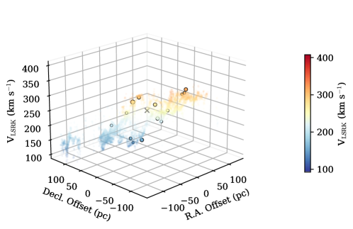
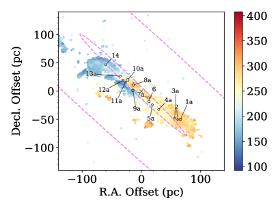
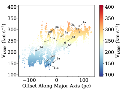
Figure 10: R.A.-Decl.-Velocity projections of the primary SSCs and CS $7-6$ in the central 280 pc of NGC 253 (the gray box in Figure 9 and the FOV of the ALMA data). Pixels with SNR < 5 in peak intensity are masked out in the CS $7-6$ velocity map. The positional offsets are calculated based on the center determined by Anantharamaiah & Goss (1996, shown as the gray $\times$ assuming this point has a velocity equal to the galaxy systemic velocity). The color scale is the same in all panels and shows the LSRK velocity. The radii of the SSC markers are $2\times r_{\rm deconv}$ (Table 1). Top: One orientation of the 3D R.A.-Decl.-Velocity view. (An animated version that rotates in azimuth is available in the online version.) Bottom left: The R.A.-Decl. projection. The pink dashed ellipses show the locations of the outermost and innermost $x_{2}$ orbits, as in Figure 9, though we note that the calculations of these orbits is highly uncertain on these scales. Bottom right: A position-velocity projection, where the positional coordinate is along the major axis of the structure shown in the bottom-left panel (PA $=235$^∘). The morphology, distribution, and kinematics of the SSCs and dense molecular gas traced by CS $7-6$ agree very well.

We compare the distribution and kinematics of the primary SSCs to CS $7-6$ observations from Krieger et al. (2019, 2020a) in Figure 10. Their cleaned cubes are a combination of 12-m, 7-m, and total power data and have a spectral resolution of 2.2 km s^-1 and a spatial resolution of 0.17″ $\times$ 0.13″ (2.9 pc $\times$ 2.2 pc). We fit the CS $7-6$ line with a Gaussian at each pixel. We mask the velocity map based on the peak intensity, where pixels with a signal-to-noise ratio (SNR) < 5 are removed. The top panel of Figure 10 shows a 3D position-position-velocity (R.A.-Decl.-Velocity) diagram of the CS $7-6$ data and the primary SSCs. The bottom row of Figure 10 shows R.A.-Decl. and position-velocity projections. The panels in Figure 10 are cropped to the FOV of the ALMA data of the SSCs described in Section 2, which cover the central 280 pc of the galaxy.

The positions and velocities of the SSCs agree well with the CS $7-6$ emitting dense molecular gas. Overplotted in the R.A.-Decl. panel of Figure 10 are the outermost and innermost $x_{2}$ orbits (pink dashed ellipses; see also Figure 9). The SSC structure and the dense molecular gas in which they are embedded are remarkably well aligned with the innermost $x_{2}$ orbits, especially given the spatial resolution of data with which the $x_{2}$ orbits were derived ($\approx$300 pc; Das et al., 2001), though there appears to be a slight PA offset. We note that the CS $7-6$ data include short- and zero-spacing data and so recover emission on large spatial scales. This means that the concentration of CS $7-6$ emission around the innermost $x_{2}$ orbit is not a result of spatial filtering by the interferometer. This is compelling evidence that the SSCs and the dense molecular gas from which they form are located at the nexus of the family of orbits which transfer gas from the bar on large scales to small scales where the gas can become dense enough to form massive young stellar clusters.

5.3 3D Structure of the SSCs and Dense Molecular Gas

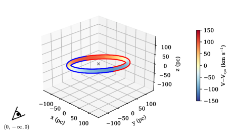
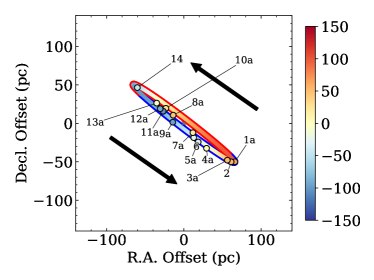
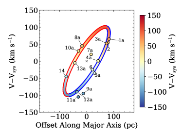
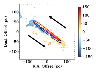
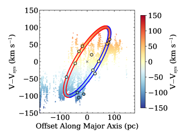
Figure 11: A model of an elliptical, angular momentum-conserving ring. Top: The ring in galactic coordinates, where $x$ corresponds to galactic longitude, $y$ to the line of sight, and $z$ to galactic latitude. The observer is at $(x,y,z)=(0,-\infty,0)$. The gray $\times$ shows the gas kinematic center. The color coding shows the radial velocity, with the galaxy systemic velocity removed. The blue (red) outlining shows the front (back) portion of the ring along the line of sight with respect to the galaxy center. (An animated version of the top panel, without the observer marked, that rotates in azimuth and elevation is available in the online version.) Middle left: The R.A.-Decl. projection of the ring with the primary SSCs overplotted. Arrows show the direction of the orbit. Middle right: A position-velocity projection of the ring and SSCs, where the positional coordinate is along the major axis of the structure (PA $=235$^∘). Bottom row: The same as the middle row, but with the CS $7-6$ plotted in the background and without the SSC labels for clarity. The arrangement and kinematics of the SSCs and CS $7-6$ are in good agreement with this simple model.

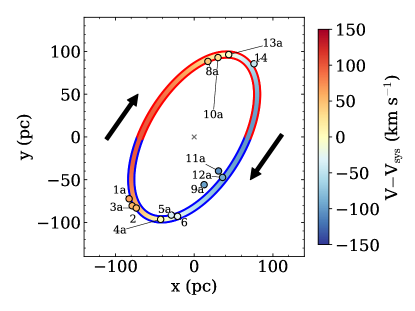
Figure 12: A top-down view of the elliptical ring model shown in the top panel of Figure 11. The observer shown in the top panel of Figure 11 is located at $(x,y)=(0,-\infty)$ in this plot. The model-dependent deprojected positions of the SSCs along this ring are shown (except for SSC 7a which is not well fit by this model). Arrows indicate the direction of the orbit. Other annotations and color-coding are as in Figure 11.

Nuclear rings following $x_{2}$ orbits are formed spontaneously in a barred potential, as revealed by hydrodynamic simulations (e.g., Tress et al., 2020), and are able to power galaxy-scale outflows (e.g., Nguyen & Thompson, 2022). $x_{2}$ orbits are mildly elongated perpendicular to the bar and have a nearly-elliptical shape. Their orbital velocity is larger at the pericenter and lower at the apocenter, qualitatively similar to what one would get by assuming that the angular momentum is constant along the orbit. Although the angular momentum is not exactly conserved along $x_{2}$ orbits (because a bar potential is non-axisymmetric — it oscillates around a mean value), a reasonable approximation is to model $x_{2}$ orbits as elliptical orbits on which the angular momentum is conserved (see also Peters, 1975). This type of model has been applied to the MW CMZ and can explain the arrangement of dense molecular gas features and star forming regions (Tress et al., 2020). In the MW, several other types of models have been developed to explain the orbits of gas, stars, and massive star-forming regions in the CMZ, including twisted rings, spirals, and crossing streams (see e.g., Henshaw et al., 2022, and references therein). We apply some of these models to the CMZ of NGC 253 in Appendix A.

5.3.1 A Plausible Model

Here, we construct a simple kinematic model of the nuclear ring in NGC 253 by assuming that the gas follows elliptical orbits on which the angular momentum is conserved. This model is built in Cartesian coordinates where the $x$-axis corresponds to galactic longitude, the $y$-axis to the line of sight from the observer, and the $z$-axis to galactic latitude (Figure 11, top). The elliptical, angular momentum-conserving ring is described by four parameters: the semi-major axis length ($a$), the semi-minor axis length ($b$), the orbital velocity at the pericenter of the ring (V_orb,0), and the position angle of the major axis of the ellipse with respect to the $x$-axis ($\theta_{p}$). The orbital velocity at every other point along the ellipse is determined by conservation of angular momentum starting from V_orb,0. The elliptical orbit in this frame is shown in the top panel of Figure 11.

To compare this model with the SSCs, we project it into the sky plane assuming some position angle (PA; defined counterclockwise of north to the receding side the the ring) and an inclination ($i$). The projection of this ring into R.A.-Decl. coordinates is shown in the left column of Figure 11. We also construct a position-velocity diagram, where the position is taken along the major axis of the ring given by the PA (Figure 11, right column).

We adjust the ring parameters by-eye to best fit the arrangement and kinematics of the SSCs. A ring with $a\sim 110$ pc, $b\sim 60$ pc, V${}_{\rm orb,0}\sim 115$ km s^-1, and $\theta_{p}\sim 55$^∘, PA $\approx 235$^∘, and $i\approx 85$^∘ is a good representation of the SSCs. We reiterate that these parameters were fit by-eye and that there are degeneracies among them. This is not meant to be an exact measurement of the size of the SSC structure, but rather to show that this is a possible configuration with reasonable parameters.

As shown in Figure 11, the SSCs agree very well with this simple model. In Figure 12, we show a top-down ("face-on") view of this ring. Using this model, we place the SSCs along the ring; the positions along the line of sight (y-axis) are entirely model dependent. Under this model, SSCs 1a, 2, 3a, 4a, 5a, 9a, 11a, and 12 would be on the front (near) side of the ring, shown as the blue outlines in Figures 11 and 12. SSCs 8a, 10a, 13a, and 14 would be on the back (far) side of the ring, shown as the red outlines.

The orbital period along the elliptical ring shown in Figures 11 and 12 is $\approx 6$ Myr. Given the limits on the SSC ages (see Section 5.4.1), this means that the SSCs have not completed a full orbit. On average, the SSCs will complete half an orbit before the massive stars within them explode as supernovae.

5.3.2 Caveats of this Simple Model

SSC 7a is not well fit by this model. Although this cluster is relatively weak compared to others, its systemic velocity was well constrained by Levy et al. (2021) and its velocity agrees well with the CS $7-6$ (Figure 10). Unlike Leroy et al. (2018) and Mills et al. (2021), we find evidence for a single velocity component towards this SSC, which may be due to the increased spatial resolution. There are multiple spatial components near SSC 7a (see e.g., Figure 1 bottom right and Figure 1 of Levy et al. 2021), which can be blended together at lower resolution leading to a second velocity component. Moreover, a shift in velocity cannot fully bring SSC 7a into agreement with the model; a change in the cluster’s velocity would shift its position vertically in position-velocity diagram (Figure 11; right column) which does not bring it into agreement with the model for reasonable adjustments to the cluster’s velocity. Because SSC 7a is not well described by this model, we do not show it in Figure 12. Hydrodynamical simulations of the MW CMZ find gas and star formation inside the CMZ ring, and it is possible that this star formation may be happening in the vicinity of the supermassive black hole Sagittarius A^∗ or associated with the nuclear star cluster (Sormani et al., 2020, and references therein). In NGC253, we also detect dense molecular gas inside the elliptical ring model (e.g., Figure 11). SSC 7a could be evidence of massive star formation close to the galactic center (whose precise position is unknown) though, with only a single cluster, this is only speculative.

Along the ring, there are more extreme radial velocities than represented by the SSCs or the dense molecular gas traced by CS $7-6$, particularly on the redshifted side of the structure (Figure 11; bottom row). In the case of the CS $7-6$ data, this is not an effect of the interferometer filtering out emission on large scales as these data include the zero-spacing (total power) data (Krieger et al., 2019, 2020a). The CS $7-6$ data cube covers LSRK velocities from 88 to 373 km s^-1, or -162 to +123 km s^-1 about the systemic velocity of the galaxy. This could mean that we are missing some of the most redshifted CS $7-6$ emission if it falls outside the bandpass. As a check, we examine the spectra in the CS $7-6$ cube, but we do not find evidence that the line profiles are cut off by the edge of the bandpass.

As noted above, simulations show that the angular momentum in an $x_{2}$ orbit is approximately constant in a time-averaged sense (e.g., Sormani et al., 2018; Tress et al., 2020). As the major-to-minor axis ratio of the orbit increases, the amplitude of the oscillations in angular momentum increase and the assumption of angular momentum conservation breaks down. For the CMZ of the MW, an $x_{2}$ orbit with an axis ratio of $110/60\approx 1.8$ would yield variations of 25% in the angular momentum over time (Sormani et al., 2018). This means that for an axis ratio like we estimate for NGC 253, the variation in angular momentum are not negligible; this is a limitation of this simple model.

As described in Section 1, we assume that the dynamical center of NGC 253 is the center determined from ionized gas kinematics by Anantharamaiah & Goss (1996). This center position has a 1-$\sigma$ uncertainty of $\sim 0.3$″, which corresponds to 5 pc. This is a negligible uncertainty in terms of the model fit shown in Figure 11, so we conclude that uncertainties in the center position determined by Anantharamaiah & Goss (1996) will not affect the results from the model. Other determinations of the dynamical center of the galaxy, however, differ by more than this measurement uncertainty. For example, the center determined from stellar kinematics by Müller-Sánchez et al. (2010) is 1.3″ (22 pc) away to the northeast in projection (between SSCs 8 and 10/11). From the standpoint of the modeling, varying the location of the dynamical center will change how the SSCs are distributed along the ring. If, for example, we instead choose the center determined by Müller-Sánchez et al. (2010), a larger ring with a higher orbital velocity is required. More challenging, however, is that a single (symmetric) ring cannot fit clusters on both the near- and far-sides of the ring simultaneously. In other words, compared to Figure 11 (right panels), a model using the center from Müller-Sánchez et al. (2010) can either fit clusters on the near (blue outlined) side of the ring or on the far (red outlined) side, but not both simultaneously. Therefore, if the true dynamical center of NGC 253 is that from Müller-Sánchez et al. (2010), then this model of a symmetric angular momentum-conserving ring is not a good fit to the data.

5.4 A Cautionary Note about SSC Ages and Age Gradients

5.4.1 Previous Estimates of the SSC Ages in NGC 253

In terms of the relative ages of the SSCs, both Rico-Villas et al. (2020) and Mills et al. (2021) found evidence for an inside-out formation scenario, where clusters towards the ends of the structure are younger and those towards the middle are older (i.e., SSCs 1, 2, 3, 13, and 14 are among the youngest and SSCs 4, 5, 7, 8, 10, 11, and 12 are among the oldest). On the other hand, Krieger et al. (2020a) used line ratios of HCN/HC₃N to construct a relative chemical age gradient, which does not follow a pattern with distance from the center and where the progression from youngest to oldest is SSC 13, 14, 1, 8, 3, 2.

The absolute ages of the SSCs in NGC 253 are highly uncertain, but limits can be placed on them. Rico-Villas et al. (2020) estimated that the SSCs in NGC 253 have ages $\approx 0.01-1$ Myr based on the ratio of luminosity of in stars (from free-free emission) and protostars. These ages are likely a lower limit, however, since the ionizing photons that produce the free-free emission may be absorbed by dust within the SSCs (see Levy et al., 2021, for a further discussion). Rico-Villas et al. (2020) also found a weak trend between their estimated ages and the HNCO/CS line ratio, where younger clusters tend to have higher line ratios. Hydrodynamical simulations of the Milky Way show that the stars and dense molecular gas are well coupled until the stars are $\sim$5 Myr old (Sormani et al., 2020). In NGC 253, the SSCs and CS $7-6$ are well matched in terms of their locations and kinematics (Figure 10), indicating that the SSCs are younger than $\sim$5 Myr. In a separate study, Mills et al. (2021) found that the clusters in NGC 253 cannot be older than $\sim 3$ Myr due to the presence of He recombination lines and the lack of appreciable synchrotron emission towards most of the clusters (indicating a lack supernovae in the SSCs). Therefore, the ages of the SSCs are likely $\sim 0.01-3$ Myr.

5.4.2 Models of Star Formation and Predictions for Age Gradients in a Circumnuclear Ring

There are three main models that describe where and when star formation occurs in a circumnuclear ring. These models make predictions for age gradients (or lack thereof) along the orbit. First, the so-called "pearls-on-a-string" scenario predicts that star formation occurs just downstream of the contact points between the gas inflow from the bar and the circumnuclear ring (i.e., downstream of the apocenters of the orbit; e.g., Böker et al. 2008; Mazzuca et al. 2008; Sormani et al. 2020). Moreover, gas in the ring will have the slowest orbital velocities at the apocenters, more easily allowing it to pile up and become dense. The star clusters age as they orbit along the ring, so the youngest clusters should be found near the apocenters with an increase in age downstream. Alternately, it has been suggested that star formation could be triggered when clouds are compressed due to close pericenter passages (Longmore et al., 2013; Kruijssen et al., 2015). Under this scenario, the youngest stars should be found closest to pericenter and stellar (or cluster) ages should increase downstream. Finally, the "popcorn" model describes a scenario in which the ring forms from gravitational collapse or turbulence and star formation is distributed uniformly along the ring (Böker et al., 2008). In this scenario, no age gradients are expected as either the clusters have approximately the same age or the ages are randomly distributed along the ring.

It is tempting to use the elliptical angular momentum conserving ring model to infer the relative ages of the SSC. However, the observations of the SSCs in NGC 253 are a single snapshot in time. Hydrodynamical simulations show that the instantaneous star formation distribution and ring morphology vary substantially about the time-averaged behavior (e.g., Tress et al., 2020; Sormani et al., 2020). While the time-averaged simulation results favor the "pearls-on-a-string" model, it is much less clear if signatures of the latter can be seen in the instantaneous simulation results due to large time-fluctuations (see especially Figure 9 of Sormani et al. 2020). Therefore, with only this single snapshot in time and a small number of SSCs, we cannot simply use the "pearls-on-a-string" (or other) model to infer the expected cluster age gradients from their locations along the elliptical ring.

6 Summary

The SSCs in the center of NGC 253 are bright continuum sources at 350 GHz, which primarily traces thermal emission from warm dust (e.g., Leroy et al., 2018; Mills et al., 2021). Here, we combine ALMA data from three 12-m configurations and the 7-m array to construct maps of the dust emission covering scales from 0.028″$-$24.8″ (0.48 pc$-$421 pc). This enables us to measure the compact dust emission associated with the clusters themselves as well as the more extended emission in which they are embedded (Figure 1). We summarize our main results below, indicating the relevant figures and/or tables.

1. For the first time, we detect the galaxy-scale outflow in dust continuum emission. As shown in Figures 1, 2, and 4, we find dust emission along the SW streamer that is located at the edge of the CO emission and hence on the exterior edge of the outflow cone. The dust streamer has a FWHM of 8 pc. From the dust, we estimate that the SW streamer has a molecular gas mass of $\sim(8-17)\times 10^{6}$ M_⊙, consistent with other measurements (e.g., Walter et al., 2017).

2. We measure the sizes of the SSCs using Gaussian fits to the cluster radial profiles. We deconvolve the Gaussian beam from the size measurements to provide beam-deconvolved cluster sizes, finding radii of $0.4-0.7$ pc (Table 1; Figures 6 and 7). Compared to star clusters in the LEGUS survey, the SSCs in NGC 253 tend to be smaller, likely because they are younger (Figure 7).

3. We investigate the morpho-kinematic arrangement of the SSCs and their possible connection to the bar. The SSC structure is on the same scale as the $x_{2}$ orbits, suggesting that gas is transported down to these scales by the bar where it can then become dense enough to form massive star-forming regions (Figures 9 and 10). We find that the SSCs have a similar distribution and kinematics as the dense molecular gas (Figure 10). We are able to describe the SSC morphology and kinematics with a simple elliptical, angular momentum-conserving model (Figures 11 and 12), which has a semi-major axis of $\sim 110$ pc, a semi-minor axis of $\sim 60$ pc, and an orbital period of $\approx 6$ Myr. From our perspective, this ring would appear nearly edge-on, leading to the observed nearly linear SSC distribution.

As described in Section 5.4.1, estimates of the (relative) SSC ages in NGC 253 do not all agree (Rico-Villas et al., 2020; Krieger et al., 2020a; Mills et al., 2021). Constraints on the absolute ages of the clusters are relatively weak, though the SSCs must be young ($\sim 0.01-3$ Myr; Rico-Villas et al. 2020; Mills et al. 2021). In the future, approved observations with the MIRI integral field unit onboard JWST will measure the ionizing radiation field of these clusters and hence provide independent constraints on the cluster ages.

Appendix A Milky Way CMZ Models Applied to NGC 253

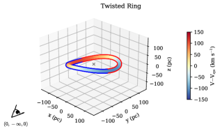
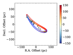
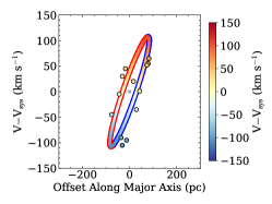
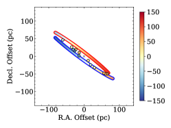
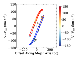
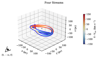
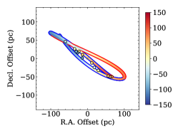
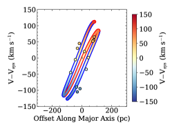
Figure 13: Similar to Figure 11, but for the CMZ models; see the caption of Figure 11 for more details. The top row shows a twisted ring model (Molinari et al., 2011), the middle row shows two spirals (e.g., Sofue, 1995; Sawada et al., 2004), and the bottom row shows a crossing streams model (Kruijssen et al., 2015).

Several models have been developed to explain the arrangement of gas and massive star-forming regions in the CMZ of the MW. Here we explore how well a naïve application of these models to NGC 253 works to represent our data. To project all of the models below into the sky plane, we assume a PA $=235$^∘ and $i=78$^∘.

A.1 Closed Orbit Models

In addition to the flat elliptical ring we explore in Section 5, another possible ring-like arrangement is a closed elliptical orbit with a vertical twist (i.e., a twisted ring Molinari et al., 2011). In the CMZ of the MW, this configuration is thought to follow the $x_{2}$ orbits and the twisted shape is induced by a vertical oscillation. The twisted ring model is described by a semi-major axis ($a$), a semi-minor axis ($b$), a constant orbital velocity (V_orb), and a vertical oscillation with an amplitude ($z_{0}$), frequency ($\nu_{z}$), and phase ($\theta_{z}$). $z_{0}$ is the amplitude of the oscillation, measured from the midplane to the peak (so the ring has a thickness of 2$\times z_{0}$. We follow Molinari et al. (2011) and assume that $\nu_{z}$ is twice the orbital frequency and $\theta_{z}=0$. Because this twisted ring model has a constant orbital velocity, it does not conserve angular momentum. This twisted ring model and the projections are shown in Figure 13 (top). The best fitting twisted ring model for the CMZ of the MW has $a=100$ pc, $b=60$ pc, $z_{0}=15$ pc, V${}_{\rm orb}=80$ km s^-1, and $\theta_{p}=-40$^∘. While such a ring in NGC 253 would have the same major- and minor-axis lengths, the amplitude of the vertical warp is $<10$ pc. Moreover, we require a higher V${}_{\rm orb}=110$ km s^-1 in NGC 253.

A.2 Open Orbit Models

As pointed out by Kruijssen et al. (2015) and others for the MW CMZ, non-circular stable closed orbits are only possible if the potential is not axisymmetric at these scales. In NGC 253, structural modeling by Leroy et al. (2015a) suggests that there are asymmetries on larger scales (as is also expected for the CMZ), but their best fitting structural model is axisymmetric on the $100-150$ pc scales we study here. We note, however, that their data are not particularly constraining on these scales due to the 35 pc resolution. Therefore, since we know the SSCs are embedded in larger-scale gas structures (e.g., Sakamoto et al., 2011; Leroy et al., 2015a; Krieger et al., 2019, 2020a, 2020b), it is perhaps more likely that the SSC orbits will be open.

One possible open-orbit model describes streams stemming from the bar-ends. Several of these kinds of models have been proposed for the CMZ in the MW (e.g., Sofue, 1995; Sawada et al., 2004; Kruijssen et al., 2015; Henshaw et al., 2016; Ridley et al., 2017; Henshaw et al., 2022). Kruijssen et al. (2015) develop a model of the MW CMZ that consists of crossing streams that form a ring-like structure. Unlike the closed ring model, this stream model is open and Sagittarius A* is located at one of the foci of the eccentric orbits. This twisted pattern precesses with time (see also Tress et al., 2020).

First we compare against a model with two spiral arms (Sofue, 1995; Sawada et al., 2004). Following Henshaw et al. (2016), we select two of the streams from the Kruijssen et al. (2015) model, and we fix their vertical positions to 0 (i.e., the streams are in the midplane). This model and the projections are shown in Figure 13 (middle).

Next, we compare against the full four-stream model developed by Kruijssen et al. (2015). To better fit the SSCs in NGC 253, we stretch this model in the $x$-direction by a factor of 1.5 and in velocity by a factor of 1.25, and we show this model in Figure 13 (bottom). Unlike any of the other models described here or in Section 5.3, this model does reproduce the position and velocity of SSC 7a; however, we cannot claim that this model is superior to others based on one SSC.

References

- Adamo et al. (2015) Adamo, A., Kruijssen, J. M. D., Bastian, N., Silva-Villa, E., & Ryon, J. 2015, MNRAS, 452, 246, doi: 10.1093/mnras/stv1203
- Adamo et al. (2017) Adamo, A., Ryon, J. E., Messa, M., et al. 2017, ApJ, 841, 131, doi: 10.3847/1538-4357/aa7132
- Anantharamaiah & Goss (1996) Anantharamaiah, K. R., & Goss, W. M. 1996, ApJ, 466, L13, doi: 10.1086/310157
- Ando et al. (2017) Ando, R., Nakanishi, K., Kohno, K., et al. 2017, ApJ, 849, 81, doi: 10.3847/1538-4357/aa8fd4
- Astropy Collaboration et al. (2018) Astropy Collaboration, Price-Whelan, A. M., Sipőcz, B. M., et al. 2018, AJ, 156, 123, doi: 10.3847/1538-3881/aabc4f
- Athanassoula (1992a) Athanassoula, E. 1992a, MNRAS, 259, 328, doi: 10.1093/mnras/259.2.328
- Athanassoula (1992b) —. 1992b, MNRAS, 259, 345, doi: 10.1093/mnras/259.2.345
- Binney et al. (1991) Binney, J., Gerhard, O. E., Stark, A. A., Bally, J., & Uchida, K. I. 1991, MNRAS, 252, 210, doi: 10.1093/mnras/252.2.210
- Binney & Tremaine (2008) Binney, J., & Tremaine, S. 2008, Galactic Dynamics: Second Edition (Princeton University Press)
- Böker et al. (2008) Böker, T., Falcón-Barroso, J., Schinnerer, E., Knapen, J. H., & Ryder, S. 2008, AJ, 135, 479, doi: 10.1088/0004-6256/135/2/479
- Bolatto et al. (2013) Bolatto, A. D., Warren, S. R., Leroy, A. K., et al. 2013, Nature, 499, 450, doi: 10.1038/nature12351
- Bolatto et al. (2021) Bolatto, A. D., Leroy, A. K., Levy, R. C., et al. 2021, ApJ, 923, 83, doi: 10.3847/1538-4357/ac2c08
- Bradley et al. (2021) Bradley, L., Sipocz, B., Robitaille, T., et al. 2021, astropy/photutils: 1.0.2, 1.0.2, Zenodo, doi: 10.5281/zenodo.4453725
- Brown & Gnedin (2021) Brown, G., & Gnedin, O. Y. 2021, MNRAS, 508, 5935, doi: 10.1093/mnras/stab2907
- Buta & Combes (1996) Buta, R., & Combes, F. 1996, Fund. Cosmic Phys., 17, 95
- Calzetti et al. (2015) Calzetti, D., Lee, J. C., Sabbi, E., et al. 2015, AJ, 149, 51, doi: 10.1088/0004-6256/149/2/51
- Caswell et al. (2020) Caswell, T. A., Droettboom, M., Lee, A., et al. 2020, matplotlib/matplotlib: REL: v3.3.2, v3.3.2, Zenodo, doi: 10.5281/zenodo.4030140
- Chandar et al. (2017) Chandar, R., Fall, S. M., Whitmore, B. C., & Mulia, A. J. 2017, ApJ, 849, 128, doi: 10.3847/1538-4357/aa92ce
- Contopoulos & Grosbol (1989) Contopoulos, G., & Grosbol, P. 1989, A&A Rev., 1, 261, doi: 10.1007/BF00873080
- Contopoulos & Mertzanides (1977) Contopoulos, G., & Mertzanides, C. 1977, A&A, 61, 477
- Das et al. (2001) Das, M., Anantharamaiah, K. R., & Yun, M. S. 2001, ApJ, 549, 896, doi: 10.1086/319430
- Davis et al. (2013) Davis, T. A., Bayet, E., Crocker, A., Topal, S., & Bureau, M. 2013, MNRAS, 433, 1659, doi: 10.1093/mnras/stt842
- Emig et al. (2020) Emig, K. L., Bolatto, A. D., Leroy, A. K., et al. 2020, ApJ, 903, 50, doi: 10.3847/1538-4357/abb67d
- Fall & Chandar (2012) Fall, S. M., & Chandar, R. 2012, ApJ, 752, 96, doi: 10.1088/0004-637X/752/2/96
- Flyamer et al. (2020) Flyamer, I., Weber/GwendalD, S., Xue, Z., et al. 2020, Phlya/adjustText: 0.8 beta, 0.8beta2, Zenodo, doi: 10.5281/zenodo.3924114
- Foreman-Mackey et al. (2013) Foreman-Mackey, D., Hogg, D. W., Lang, D., & Goodman, J. 2013, PASP, 125, 306, doi: 10.1086/670067
- Galliano et al. (2008) Galliano, F., Dwek, E., & Chanial, P. 2008, ApJ, 672, 214, doi: 10.1086/523621
- Gao & Solomon (2004) Gao, Y., & Solomon, P. M. 2004, ApJS, 152, 63, doi: 10.1086/383003
- Gieles et al. (2006) Gieles, M., Larsen, S. S., Scheepmaker, R. A., et al. 2006, A&A, 446, L9, doi: 10.1051/0004-6361:200500224
- Goldreich & Tremaine (1979) Goldreich, P., & Tremaine, S. 1979, ApJ, 233, 857, doi: 10.1086/157448
- Gorski et al. (2017) Gorski, M., Ott, J., Rand, R., et al. 2017, ApJ, 842, 124, doi: 10.3847/1538-4357/aa74af
- Gorski et al. (2019) Gorski, M. D., Ott, J., Rand, R., et al. 2019, MNRAS, 483, 5434, doi: 10.1093/mnras/sty3077
- Grudić et al. (2021) Grudić, M. Y., Guszejnov, D., Hopkins, P. F., Offner, S. S. R., & Faucher-Giguère, C.-A. 2021, MNRAS, 506, 2199, doi: 10.1093/mnras/stab1347
- Haasler et al. (2022) Haasler, D., Rivilla, V. M., Martín, S., et al. 2022, A&A, 659, A158, doi: 10.1051/0004-6361/202142032
- Harris et al. (2020) Harris, C. R., Millman, K. J., van der Walt, S. J., et al. 2020, Nature, 585, 357, doi: 10.1038/s41586-020-2649-2
- Heckman et al. (2000) Heckman, T. M., Lehnert, M. D., Strickland , D. K., & Armus, L. 2000, ApJS, 129, 493, doi: 10.1086/313421
- Heesen et al. (2011) Heesen, V., Beck, R., Krause, M., & Dettmar, R. J. 2011, A&A, 535, A79, doi: 10.1051/0004-6361/201117618
- Henshaw et al. (2022) Henshaw, J. D., Barnes, A. T., Battersby, C., et al. 2022
- Henshaw et al. (2016) Henshaw, J. D., Longmore, S. N., Kruijssen, J. M. D., et al. 2016, MNRAS, 457, 2675, doi: 10.1093/mnras/stw121
- Hollyhead et al. (2016) Hollyhead, K., Adamo, A., Bastian, N., Gieles, M., & Ryon, J. E. 2016, MNRAS, 460, 2087, doi: 10.1093/mnras/stw1142
- Humire et al. (2022) Humire, P. K., Henkel, C., Hernández-Gómez, A., et al. 2022, arXiv e-prints, arXiv:2205.03281. https://arxiv.org/abs/2205.03281
- Johnson et al. (2017) Johnson, L. C., Seth, A. C., Dalcanton, J. J., et al. 2017, ApJ, 839, 78, doi: 10.3847/1538-4357/aa6a1f
- King (1962) King, I. 1962, AJ, 67, 471, doi: 10.1086/108756
- Klein et al. (2018) Klein, A., Silvester, S., Tanbakuchi, A., et al. 2018, imageio/imageio: V2.4.1, v2.4.1, Zenodo, doi: 10.5281/zenodo.1488562
- Knapen (1999) Knapen, J. H. 1999, in Astronomical Society of the Pacific Conference Series, Vol. 187, The Evolution of Galaxies on Cosmological Timescales, ed. J. E. Beckman & T. J. Mahoney, 72–87. https://arxiv.org/abs/astro-ph/9907290
- Koribalski et al. (2004) Koribalski, B. S., Staveley-Smith, L., Kilborn, V. A., et al. 2004, AJ, 128, 16, doi: 10.1086/421744
- Kormendy & Kennicutt (2004) Kormendy, J., & Kennicutt, Robert C., J. 2004, ARA&A, 42, 603, doi: 10.1146/annurev.astro.42.053102.134024
- Kornei & McCrady (2009) Kornei, K. A., & McCrady, N. 2009, ApJ, 697, 1180, doi: 10.1088/0004-637X/697/2/1180
- Krieger et al. (2019) Krieger, N., Bolatto, A. D., Walter, F., et al. 2019, ApJ, 881, 43, doi: 10.3847/1538-4357/ab2d9c
- Krieger et al. (2020a) Krieger, N., Bolatto, A. D., Leroy, A. K., et al. 2020a, ApJ, 897, 176, doi: 10.3847/1538-4357/ab9c23
- Krieger et al. (2020b) Krieger, N., Bolatto, A. D., Koch, E. W., et al. 2020b, ApJ, 899, 158, doi: 10.3847/1538-4357/aba903
- Kruijssen et al. (2015) Kruijssen, J. M. D., Dale, J. E., & Longmore, S. N. 2015, MNRAS, 447, 1059, doi: 10.1093/mnras/stu2526
- Krumholz & Kruijssen (2015) Krumholz, M. R., & Kruijssen, J. M. D. 2015, MNRAS, 453, 739, doi: 10.1093/mnras/stv1670
- Krumholz et al. (2019) Krumholz, M. R., McKee, C. F., & Bland -Hawthorn, J. 2019, ARA&A, 57, 227, doi: 10.1146/annurev-astro-091918-104430
- Leroy et al. (2015a) Leroy, A. K., Bolatto, A. D., Ostriker, E. C., et al. 2015a, ApJ, 801, 25, doi: 10.1088/0004-637X/801/1/25
- Leroy et al. (2015b) Leroy, A. K., Walter, F., Martini, P., et al. 2015b, ApJ, 814, 83, doi: 10.1088/0004-637X/814/2/83
- Leroy et al. (2018) Leroy, A. K., Bolatto, A. D., Ostriker, E. C., et al. 2018, ApJ, 869, 126, doi: 10.3847/1538-4357/aaecd1
- Levy et al. (2021) Levy, R. C., Bolatto, A. D., Leroy, A. K., et al. 2021, ApJ, 912, 4, doi: 10.3847/1538-4357/abec84
- Longmore et al. (2013) Longmore, S. N., Kruijssen, J. M. D., Bally, J., et al. 2013, MNRAS, 433, L15, doi: 10.1093/mnrasl/slt048
- Mangum et al. (2013) Mangum, J. G., Darling, J., Henkel, C., et al. 2013, ApJ, 779, 33, doi: 10.1088/0004-637X/779/1/33
- Martín et al. (2021) Martín, S., Mangum, J. G., Harada, N., et al. 2021, A&A, 656, A46, doi: 10.1051/0004-6361/202141567
- Mazzuca et al. (2008) Mazzuca, L. M., Knapen, J. H., Veilleux, S., & Regan, M. W. 2008, ApJS, 174, 337, doi: 10.1086/522338
- McCormick et al. (2013) McCormick, A., Veilleux, S., & Rupke, D. S. N. 2013, ApJ, 774, 126, doi: 10.1088/0004-637X/774/2/126
- McMullin et al. (2007) McMullin, J. P., Waters, B., Schiebel, D., Young, W., & Golap, K. 2007, in Astronomical Society of the Pacific Conference Series, Vol. 376, Astronomical Data Analysis Software and Systems XVI, ed. R. A. Shaw, F. Hill, & D. J. Bell, 127
- Meier et al. (2015) Meier, D. S., Walter, F., Bolatto, A. D., et al. 2015, ApJ, 801, 63, doi: 10.1088/0004-637X/801/1/63
- Messa et al. (2018a) Messa, M., Adamo, A., Östlin, G., et al. 2018a, MNRAS, 473, 996, doi: 10.1093/mnras/stx2403
- Messa et al. (2018b) Messa, M., Adamo, A., Calzetti, D., et al. 2018b, MNRAS, 477, 1683, doi: 10.1093/mnras/sty577
- Mills et al. (2021) Mills, E. A. C., Gorski, M., Emig, K. L., et al. 2021, ApJ, 919, 105, doi: 10.3847/1538-4357/ac0fe8
- Mok et al. (2019) Mok, A., Chandar, R., & Fall, S. M. 2019, ApJ, 872, 93, doi: 10.3847/1538-4357/aaf6ea
- Mok et al. (2020) —. 2020, ApJ, 893, 135, doi: 10.3847/1538-4357/ab7a14
- Molinari et al. (2011) Molinari, S., Bally, J., Noriega-Crespo, A., et al. 2011, ApJ, 735, L33, doi: 10.1088/2041-8205/735/2/L33
- Müller-Sánchez et al. (2010) Müller-Sánchez, F., González-Martín, O., Fernández-Ontiveros, J. A., Acosta-Pulido, J. A., & Prieto, M. A. 2010, ApJ, 716, 1166, doi: 10.1088/0004-637X/716/2/1166
- Nguyen & Thompson (2022) Nguyen, D. D., & Thompson, T. A. 2022, arXiv e-prints, arXiv:2205.13465. https://arxiv.org/abs/2205.13465
- Ossenkopf & Henning (1994) Ossenkopf, V., & Henning, T. 1994, A&A, 291, 943
- Paglione et al. (2004) Paglione, T. A. D., Yam, O., Tosaki, T., & Jackson, J. M. 2004, ApJ, 611, 835, doi: 10.1086/422354
- Pence (1980) Pence, W. D. 1980, ApJ, 239, 54, doi: 10.1086/158088
- Pérez-Ramírez et al. (2000) Pérez-Ramírez, D., Knapen, J. H., Peletier, R. F., et al. 2000, MNRAS, 317, 234, doi: 10.1046/j.1365-8711.2000.03521.x
- Peters (1975) Peters, W. L., I. 1975, ApJ, 195, 617, doi: 10.1086/153363
- Plummer (1911) Plummer, H. C. 1911, MNRAS, 71, 460, doi: 10.1093/mnras/71.5.460
- Portegies Zwart et al. (2010) Portegies Zwart, S. F., McMillan, S. L. W., & Gieles, M. 2010, ARA&A, 48, 431, doi: 10.1146/annurev-astro-081309-130834
- Reback et al. (2020) Reback, J., McKinney, W., jbrockmendel, et al. 2020, pandas-dev/pandas: Pandas 1.1.3, v1.1.3, Zenodo, doi: 10.5281/zenodo.4067057
- Regan & Teuben (2003) Regan, M. W., & Teuben, P. 2003, ApJ, 582, 723, doi: 10.1086/344721
- Rekola et al. (2005) Rekola, R., Richer, M. G., McCall, M. L., et al. 2005, MNRAS, 361, 330, doi: 10.1111/j.1365-2966.2005.09166.x
- Rico-Villas et al. (2020) Rico-Villas, F., Martín-Pintado, J., González-Alfonso, E., Martín, S., & Rivilla, V. M. 2020, MNRAS, 491, 4573, doi: 10.1093/mnras/stz3347
- Ridley et al. (2017) Ridley, M. G. L., Sormani, M. C., Treß, R. G., Magorrian, J., & Klessen, R. S. 2017, MNRAS, 469, 2251, doi: 10.1093/mnras/stx944
- Rohatgi (2021) Rohatgi, A. 2021, Webplotdigitizer: Version 4.5. https://automeris.io/WebPlotDigitizer
- Sakamoto et al. (2011) Sakamoto, K., Mao, R.-Q., Matsushita, S., et al. 2011, ApJ, 735, 19, doi: 10.1088/0004-637X/735/1/19
- Sawada et al. (2004) Sawada, T., Hasegawa, T., Handa, T., & Cohen, R. J. 2004, MNRAS, 349, 1167, doi: 10.1111/j.1365-2966.2004.07603.x
- Scoville et al. (1985) Scoville, N. Z., Soifer, B. T., Neugebauer, G., et al. 1985, ApJ, 289, 129, doi: 10.1086/162871
- Sharp & Bland-Hawthorn (2010) Sharp, R. G., & Bland-Hawthorn, J. 2010, ApJ, 711, 818, doi: 10.1088/0004-637X/711/2/818
- Shin et al. (2017) Shin, J., Kim, S. S., Baba, J., et al. 2017, ApJ, 841, 74, doi: 10.3847/1538-4357/aa7061
- Sofue (1995) Sofue, Y. 1995, PASJ, 47, 527. https://arxiv.org/abs/astro-ph/9508110
- Sofue & Rubin (2001) Sofue, Y., & Rubin, V. 2001, ARA&A, 39, 137, doi: 10.1146/annurev.astro.39.1.137
- Sorai et al. (2000) Sorai, K., Nakai, N., Kuno, N., Nishiyama, K., & Hasegawa, T. 2000, PASJ, 52, 785, doi: 10.1093/pasj/52.5.785
- Sormani et al. (2018) Sormani, M. C., Sobacchi, E., Fragkoudi, F., et al. 2018, MNRAS, 481, 2, doi: 10.1093/mnras/sty2246
- Sormani et al. (2020) Sormani, M. C., Tress, R. G., Glover, S. C. O., et al. 2020, MNRAS, 497, 5024, doi: 10.1093/mnras/staa1999
- Sormani et al. (2022) Sormani, M. C., Sanders, J. L., Fritz, T. K., et al. 2022, MNRAS, 512, 1857, doi: 10.1093/mnras/stac639
- Strickland et al. (2000) Strickland, D. K., Heckman, T. M., Weaver, K. A., & Dahlem, M. 2000, AJ, 120, 2965, doi: 10.1086/316846
- Strickland et al. (2002) Strickland, D. K., Heckman, T. M., Weaver, K. A., Hoopes, C. G., & Dahlem, M. 2002, ApJ, 568, 689, doi: 10.1086/338889
- Sturm et al. (2011) Sturm, E., González-Alfonso, E., Veilleux, S., et al. 2011, ApJ, 733, L16, doi: 10.1088/2041-8205/733/1/L16
- Sugai et al. (2003) Sugai, H., Davies, R. I., & Ward, M. J. 2003, ApJ, 584, L9, doi: 10.1086/368271
- Tress et al. (2020) Tress, R. G., Sormani, M. C., Glover, S. C. O., et al. 2020, MNRAS, 499, 4455, doi: 10.1093/mnras/staa3120
- Turner & Ho (1985) Turner, J. L., & Ho, P. T. P. 1985, ApJ, 299, L77, doi: 10.1086/184584
- Ulvestad & Antonucci (1997) Ulvestad, J. S., & Antonucci, R. R. J. 1997, ApJ, 488, 621, doi: 10.1086/304739
- van Albada & Sanders (1982) van Albada, T. S., & Sanders, R. H. 1982, MNRAS, 201, 303, doi: 10.1093/mnras/201.2.303
- Van Rossum (2020) Van Rossum, G. 2020, The Python Library Reference, release 3.8.2 (Python Software Foundation)
- Virtanen et al. (2020) Virtanen, P., Gommers, R., Oliphant, T. E., et al. 2020, Nature Methods, 17, 261, doi: 10.1038/s41592-019-0686-2
- Wada & Habe (1992) Wada, K., & Habe, A. 1992, MNRAS, 258, 82, doi: 10.1093/mnras/258.1.82
- Walter et al. (2017) Walter, F., Bolatto, A. D., Leroy, A. K., et al. 2017, ApJ, 835, 265, doi: 10.3847/1538-4357/835/2/265
- Waskom et al. (2014) Waskom, M., Botvinnik, O., Hobson, P., et al. 2014, Seaborn: V0.5.0 (November 2014), v0.5.0, Zenodo, doi: 10.5281/zenodo.12710
- Watson et al. (1996) Watson, A. M., Gallagher, J. S., I., Holtzman, J. A., et al. 1996, AJ, 112, 534, doi: 10.1086/118032
- Weiß et al. (2008) Weiß, A., Kovács, A., Güsten, R., et al. 2008, A&A, 490, 77, doi: 10.1051/0004-6361:200809909
- Westmoquette et al. (2011) Westmoquette, M. S., Smith, L. J., & Gallagher, J. S., I. 2011, MNRAS, 414, 3719, doi: 10.1111/j.1365-2966.2011.18675.x
- Whitmore et al. (2010) Whitmore, B. C., Chandar, R., Schweizer, F., et al. 2010, AJ, 140, 75, doi: 10.1088/0004-6256/140/1/75
- Zhang & Fall (1999) Zhang, Q., & Fall, S. M. 1999, ApJ, 527, L81, doi: 10.1086/312412
- Zschaechner et al. (2018) Zschaechner, L. K., Bolatto, A. D., Walter, F., et al. 2018, ApJ, 867, 111, doi: 10.3847/1538-4357/aadf32