Lessons from the Magellanic System and its modeling

Abstract

The prominent Magellanic Stream that dominates the HI sky provides a tantalizing number of observations that potentially constrains the Magellanic Clouds and the Milky Way outskirts. Here we show that the ’ram-pressure plus collision’ model naturally explain these properties, and is able to predict some of the most recent observations made after the model was made. These include the complexity of the stellar populations in the Magellanic Bridge, for which kinematics, ages, and distances are well measured, and the Northern Tidal Arm, for which the model predicts its formation from the Milky Way tidal forces. It appears that this over-constrained model provides a good path to investigate the Stream properties. This contrasts with tidal models that reproduce only half of the Stream’s main properties, in particular a tidal tail cannot reproduce the observed inter-twisted filaments, and its gas content is not sufficiently massive to provide the large amount of HI and HII gas associated to the Stream. Despite the efforts made to reproduce the large amounts of gas brought by the Clouds, it seems that no viable solution for the tidal model could be foreseen. Since the ’ram-pressure plus collision’ model has not succeeded for a Large Magellanic Cloud mass above 2 $\times 10^{10}$ $M_{\odot}$, we conjecture that a low mass is required to form the Stream.

1 Introduction

Together, the Magellanic Stream (MS) and Leading Arm (LA) subtend an angle of 230 degree, making it the second most prominent neutral hydrogen structure dominating the sky, after the Milky Way. The MS has been identified to be anchored to the Magellanic Clouds in 1974 by Mathewson, Cleary & Murray (1974), though the nature of its formation was considered still unknown in 2012 (Mathewson, 2012). HST proper motion measurements of the Magellanic Clouds by (Kallivayalil et al., 2006; Piatek, Pryor & Olszewski, 2008; Kallivayalil et al., 2013) indicate that the Clouds are presently moving at high velocities, and are consistent with a first passage about the Galaxy (Besla et al., 2007). In such a frame, modeling of the MS has followed two very different and mutually exclusive schemes, since either it can be a tidal tail (Besla et al., 2012, and references therein), or it can be made by one or two ram-pressure tails (Mastropietro, 2010; Hammer et al., 2015).

Today the most influential tidal model of the MS is that of Besla et al. (2012), for which the MS is a gigantic tidal tail extracted from the Small Magellanic Cloud (SMC) by the tidal effect of the Large Magellanic Cloud (LMC) during a close interaction 1.2 to 2 Gyr ago. The SMC is further assumed to be a long-lived satellite of the LMC, which imposes a very large mass for the latter, in excess of $10^{11}$ $M_{\odot}$ (Kallivayalil et al., 2013). The strengths of the Besla et al. (2012) model are their predictions of the MS length, of the 6 D space-velocity phase of the Clouds, and that it predicts at least one arm of the LA.

The major limitations of the Besla et al. (2012) tidal model include (i) that only a small fraction, few percent, of the MS gas is reproduced, and no ionized gas while it is the prominent component of the MS (Fox et al., 2014), (ii) the stream is made of two filaments, with kinematic and chemical analyses indicating that gas from both the LMC and SMC is present, and (iii) the absence of stars in the Stream observed so far. Each of these limitations appear to be a showstopper for the tidal model of the MS.

The Besla et al. (2012) model is also limited because it neglects the presence of a coronal phase in the Milky Way (MW) halo, while the presence of a multi-phase circumgalactic medium (CGM) has been evidenced by many means (X-rays: Bregman et al. 2018; Faerman, Sternberg & McKee 2017; Miller & Bregman 2013; QSO absorption lines: Zheng et al. 2015, 2019; Fox et al. 2014; Richter et al. 2017; LMC shrunk gas disk: Nidever 2014; high velocity cloud dissociation: Kalberla & Haud 2006). More recent realizations of the tidal model have introduced the MW coronal phase together with that of a putative LMC corona (Lucchini et al., 2020; Lucchini, D’Onghia & Fox, 2021).

Compared to tidal models, the ’ram-pressure plus collision’ model (Hammer et al., 2015; Wang et al., 2019) appears much more advanced since it reproduces in details many known properties of the MS, as well as some qualitative. In this model the LA is produced by the leading passages of gas-rich dwarfs assumed to be progenitors of present-day MW dwarfs (see also Tepper-García et al. 2019). This hypothesis has been also adopted by the most recent tidal model of the MS (Lucchini, D’Onghia & Fox, 2021), and is further supported by the MW dwarf high energies and angular momenta, suggesting also a recent passage for them (Hammer et al., 2021). By construction, the ’ram-pressure plus collision’ model reproduces the dual filamentary structures, which are two ram-pressure tails attached to each Clouds, the whole HI MS shape and gas mass and its radial velocity (Hammer et al., 2015). The recent collision between the Clouds explains the Magellanic Bridge, leading to Cloud proper motions consistent with the observed values. It also reproduces the velocity field of the LMC and the gigantic, 30 kpc-long, structure along the line of sight of the SMC young stars (Wang et al., 2019; Ripepi et al., 2017), which both are due to the recent, 300 Myr old, collision between the gas-rich Clouds. Moreover, the MS ionized gas deposited during the MC motions in the MW halo is coming from the HI gas of the Clouds, which has been extracted by ram-pressure, and then ionized by the hot corona of the MW (Wang et al., 2019).

However and quite surprisingly, the ’ram-pressure plus collision’ model does not assume a dark matter component for both Clouds, while it naturally reproduces the MS in details without fine-tuning. It even constrains the LMC mass to be smaller than 2 $\times 10^{10}$ $M_{\odot}$, because otherwise it would not let sufficient expelled gas to make the mass of the HI and especially that of the HII MS. This may come at odd with LMC mass estimates based on the interaction between the MW and the LMC (Erkal et al., 2019, 2021; Conroy et al., 2021; Vasiliev, Belokurov & Erkal, 2021).

In this paper we aim at testing the ’ram-pressure plus collision’ model by considering the most recent and new constraints on the Magellanic System. The tests include the morphological-age-kinematics distribution of stars in the Magellanic Bridge (MB), and the morphological and kinematic behavior of the faint Northern Tidal Arm (NTA), which stretch an angle of 12.5 degree. In principle, the tantalizing number of observations that are reproduced makes this model over-constrained and hence, able to be predictive. The paper is organized as it follows. In section 2, we describe the observational properties of two populations identified in the MB region, the ’ram-pressure plus collision’ model from Wang et al. (2019), comparison between MB stellar populations and predictions from the simulations ,as well as an interpretation of their origin. In section 3, we compare the Gaia results for the NTA with our simulation model predictions. In section 4, we discuss the advantages and inconveniences of the different Magellanic System modeling, and then conclude in section 5.

2 The two stellar populations in the Magellanic Bridge

2.1 Additional constraints from the Bridge

In the MB region, the neutral gas bridge has been well identified by HI observations (Nidever et al., 2010), which well elucidate the mutual interaction between MCs. A population of young stars in the Bridge has been also identified by various observations (Irwin, Kunkel & Demers, 1985; Demers & Battinelli, 1998), and their strong correlation with the MB neutral gas indicates that they likely result from in-situ star-formation during the recent MC interaction (Skowron et al., 2014; Belokurov et al., 2017).

Besides young stars in the Bridge region, older age RGB stars have been also discovered by Bagheri, Cioni & Napiwotzki (2013) and Noël et al. (2013), and Skowron et al. (2014) identified the presence of red clump stars as well. These older age stars are either distributed with a large scatter in the Bridge region or in front of the gas Bridge region with respect to the motion direction (see also Belokurov et al. 2017).

Recent observations of the MB have confirmed stellar populations with ages ranging from Young Main Sequence stars and old ancient RR Lyrae (Belokurov et al., 2017). Based on star formation and orbital past histories of the Clouds, the MB has been formed $\sim 200-300$ Myr ago (Casetti-Dinescu et al., 2012; Hammer et al., 2015). Thanks to the $Gaia$ precise proper motion data, stellar tangential motions have been measured in the MB region, revealing that stars in the MB are leaving SMC towards the LMC (Belokurov et al., 2017; Gaia Collaboration et al., 2021; Omkumar et al., 2021; Zivick et al., 2019; Schmidt et al., 2020). It suggests that they have been stripped from the SMC due to the LMC tidal force. By using the red clump (RC) as standard candle, Nidever et al. (2013) found that there are two stellar populations with different brightnesses within the MB, which has been recently confirmed by Omkumar et al. (2021). With $Gaia$ DR2 data, Omkumar et al. (2021) found that the bright star population at the SMC distance has a larger tangential velocity than the fainter, more distant population. This observation may provide a useful constraint for models to simulate the formation of Magellanic System.

2.2 Comparison between simulated data and observations

2.2.1 The ram-pressure plus collision model

Wang et al. (2019) adapted a ”ram-pressure plus collision” model to reproduce the MS and MCs formation using the state-of-the-art software GIZMO (Hopkins, 2015). In this model the MS is formed by an interaction between MCs and ram-pressure exerted by the Milky Way hot corona. It leads to dual HI streams behind each MCs, and explains the kinematics and the mass of the huge amount of ionized gas kinematically coupled with the MS. Besides this, the strong interaction between MCs tidally reshapes SMC to a very elongated structure.

In the model of Wang et al. (2019), the stellar distribution of SMC consists of a disk and a spheroid components. The stellar disk is an exponential distribution with scalelength 1.5 kpc, and the spheroid component follows the profile of Dehnen (1993) with $\gamma=0$, which has a core in the center with half mass radius 5.8 kpc. The stellar disk represents the young star population observed in the SMC, while the extended spheroid component is motivated by the spheroidal distribution of ancient RR Lyrae stars observed around the SMC (Ripepi et al., 2017). This model of the SMC have been shown to reproduce well the very extended cylindrical structure with line-of-sight distance around 30 kpc for young stars, as well as the nearly spheroidal distribution of RR Lyrae stars (Ripepi et al., 2017; Scowcroft et al., 2016; Wang et al., 2019). Wang et al. (2019) discussed all details for the initial conditions and modeling.

To compare the 3D morphology of MCs with RR Lyrae data and Classic Cepheid observed in Ripepi et al. (2017), Wang et al. (2019) have randomly selected particles to match the numbers to the observed stars, and to match the observed region. This renders it difficult to distinguish the faint features around MCs, especially in the Magellanic Bridge region as shown in Fig. 7 of Wang et al. (2019).

Here, to have a view of the whole particle distribution in 3D space, we now show in Fig.1 the simulated MCs particles distribution with all of particles used in our simulation model of Wang et al. (2019). The green color dots indicate the LMC particles, while the cyan color dots represent the SMC. In this figure, particles distribute over a much larger region than in Fig.7 of Wang et al. (2019), which illustrates well that the MB is connecting both MCs.

2.2.2 Two stellar populations at different distances in the Bridge

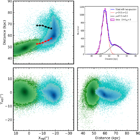
Figure 1: Simulated particles distributions of LMC and SMC in Magellanic Bridge coordinates (Belokurov et al., 2017) (bottom-left), or Magellanic Bridge longitude/latitude versus distance (bottom-right and top-left, respectively). Greens (cyan) points are particles from LMC (SMC). In the top-left panel, the red and black big stars indicates the mean distance values along Magellanic Bridge longitude for the background and foreground population, which are separated at 60 kpc. The top-right panel indicates the distance distribution for stars within the Bridge region, to which are overplotted two Gaussian functions fitted to this distribution and the fitted results are labeled on this panel.

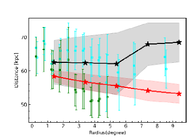
Figure 2: Comparing relations of distances varied with radius to the SMC between observation and simulations. Green and cyan color indicate bright and faint population of RC from Omkumar et al. (2021) for North East (solid square) and South East region (open square). Simulation data from Model-52 are shown by red and red stars, and the gray and pink region shown the 1$\sigma$ distance scatter.

Figure 3: Particles distributions in the MB longitude, latitude, and distance space. The left panels show spheroid component of SMC and the right panels present the disk component of SMC. The black and red stars indicate the mean distance along with the MB longitude for stars separated at 60 kpc.

Fig. 1 presents the whole star particle distribution in Magellanic Bridge coordinates (Belokurov et al., 2017) and also identifies their distances. In Fig. 1 all particles are shown and their colors identify whether they belong to the LMC (green) or to the SMC (cyan). In the X_MB versus distance panel (top left panel), there is a tidal bridge (red dots) connecting LMC to SMC with distance varying from $\sim$ 65 kpc (SMC) to $\sim$ 50 kpc (LMC), which forms the stellar Magellanic Bridge (MB). Behind the MB, there are particles of SMC distributed from 60 kpc to 80 kpc, which originated from the SMC after tidal interaction with LMC. The MB and background populations of SMC are clearly separated in distance.

In the top right panel of Fig. 1 the distance distribution of particles within $-15{\degr}\la{\rm X_{MB}}\la-8{\degr}$ are shown with a magenta line. There are two populations with different distances distribution. Two Gaussian functions (red-dashed and black-dashed lines) are used to fit these two populations, and the results for the mean and standard deviation of distance are labeled on the top right of this panel. The two populations are clearly located at two different distances, one at $\sim 55$ kpc that delineates the mean value of the MB, the other one having a broader distance distribution with a mean value of $\sim 67$ kpc. The two populations are well separated at $\sim 60$ kpc.

Omkumar et al. (2021) used RC stars to trace distance and found that the stellar population in the East part of SMC have two different populations at different distances. To better compare with observation data, we fitted two Gaussian functions with distance distribution for different MB longitude bins. The fitted results are shown in the Fig. 11 of Appendix. All of the distance distributions at different bins are well fitted with two Gaussian functions. We note that the foreground population between 50 and 60 kpc is the dominant component for all the distribution bins, while it is less prominent in the observation (see figure 4 of Omkumar et al., 2021). This indicates that the interaction between LMC and SMC is so strong in the simulation that too many particles are tidally stripped from the SMC. A fine tuning model parameters is needed to reduce this component to match with observation. For example, this can be done by either increasing the pericenter to decrease the tidal force, or by decreasing the size or the mass of the SMC disk component, or to change the SMC inclination angle relatively to the orbital plan in order to decrease resonance.

Fig.2 compares the distance variation at different SMC radii for the two components, allowing to compare observation data and simulation results. The observed data are shown in green (bright RC population) and cyan (faint RC population), with solid squares for the North East and open squares for the South East. The two Gaussian fitted results to the simulation data are shown with red (foreground population) and black (background population) colors. The simulated foreground population follow the trends that its distance decreases with increasing SMC radius, which matches with the observed bright RC (green square) population. The background population in the simulation has a nearly flat distance distribution at radii less than $\la 7\degr$, and the distance increases at radii $\ga 7\degr$, which is roughly similar to the faint RC population.

In our model, the progenitor of SMC consists of a disk and a spheroid component (Wang et al., 2019). In Fig. 3 the spheroid (left panels) and disk (right panels) components of SMC are separated and shown in the MB coordinates or longitude/latitude versus distance. The background population are mainly coming from the spheroidal component, while the foreground component includes contributions from both the spheroid and the disk component.

2.2.3 Kinematic features for the two populations

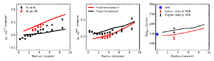
Figure 4: The relative variation of proper motions with respect to that of SMC as function of radius to SMC are shown in left and middle panels, and the right panel shows the radial velocity variation as function of radii to SMC. The observed proper motions and radial velocity of SMC are from Zivick et al. (2018). The proper motion of faint (black square) and bright (red square) RC in the left and middle panel are from Omkumar et al. (2021). The radial velocity of the lower (red circles) and higher (black circles) velocity RGB stars are from James et al. (2021), which are corresponds to foreground components and main body of SMC.

Using $Gaia$ DR2, Omkumar et al. (2021) studied the proper motions of these two populations, and found two populations with different kinematics. They identified the proper motions of the two populations in both directions (${\mu}_{\alpha}$, ${\mu}_{\delta}$) as well as their variations against the SMC radius.

Left and middle panels of Fig.4 show the relative proper motions variation of the two populations with respected to SMC as function of radius to SMC. The background (faint) and foreground (bright) RC are shown with black and red squares, while the modelled background and foreground are shown with black and red solid lines. The background (faint) RC component has been argued to belong to the main body of SMC (Omkumar et al., 2021; James et al., 2021), but this has to be clarified. This is because there are systematic differences ($\sim 0.16$ mas/yr) of ${\mu}_{\alpha}$ and ${\mu}_{\delta}$ near the central regions (see black squares at zero radius in left and middle panels of Fig.4. The modeled proper motions reproduce qualitatively the observations by many aspects, including the variations of proper motions in both directions with the SMC radius. Both observations and simulations show that the foreground population has larger $\mu_{\alpha}$ than the background population (left panel), and that this relation is inverted in the $\mu_{\delta}$ (middle panel). The right panel of Fig.4 shows the radial velocity as function of radius for the model. Both the background and foreground population shows increasing velocity with increasing radius, namely it increases toward to LMC. The background population have higher radial velocity than foreground population. With $Gaia$ EDR3 and collected radial velocity data from literature, James et al. (2021) identified two radial velocity components in the eastern region of SMC for the RGB stars with velocity difference by $\sim 35-45$ km/s. The higher (lower) radial velocity component has proper motions consistent with the background (foreground) RC population. This suggests that the lower velocity component belongs to the same substructure than the foreground population, and the higher velocity component corresponds to the main body of SMC as well as the background component. In the right panel of Fig.4 the two radial velocity components of RGB from James et al. (2021) are shown by black and red circles. Even though the difference of radial velocity between background and foreground in our model is smaller than that observed, our model correctly predicts that the foreground component has a lower velocity than that in thebackground.

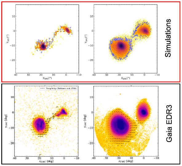
Figure 5: Comparing the young and old population bridge between simulation model and $Gaia$ EDR3 data. Vector field are overlapped on the density maps for young stars (left panels) and old stars (right panels). The coordinates has been centered on SMC for comparison with new results from $Gaia$ EDR3 (Gaia Collaboration et al., 2021). There is clearly young star bridge connecting LMC and SMC, and moving toward to the LMC, which are consistent with the $Gaia$ EDR3 results (bottom panel) for both density map and velocity vector (Gaia Collaboration et al., 2021). There is also old stellar bridge for the observation and simulation results. Since there are no quantitative length scale of proper motion vector available for the observation data from Gaia Collaboration et al. (2021), the length scale of arrows are not matched between observation and model.

Gaia Collaboration et al. (2021) have confirmed the above observational results with $Gaia$ EDR3 data, showing that there are both young and old stellar bridge having both their proper motions towards the LMC. To have a comparison, we selected young population as required stars with age smaller than 150 Myr, and old stars with age larger than 2 Gyr which are corresponding to the intermediate-old red clump population used in Gaia Collaboration et al. (2021). The top left-panel of Fig.5 shows the young stars distribution on the sky, and the blue arrows indicate the proper motion vector with respect to SMC. In the top right-panel of Fig.5 the old population shows a bridge connection between the LMC and the SMC, which has proper motions similar to that of young stars moving from the two Clouds. For comparison, data from $Gaia$ EDR3 are shown in the bottom panels of Fig.5 from Gaia Collaboration et al. (2021). Both young and old population in the Bridge region share similar motion properties for both observations and model, in particular the Bridge star motions towards the LMC. Only qualitative comparison is feasible because there is no available length scale for the proper motion vectors in the observation data from Gaia Collaboration et al. (2021). Even though these qualitative comparisons indicate the model reproduce well the observation proper motions, there is one difference between the model and data. For example, the proper motions of outskirts of the LMC have a bottom-right bulk motion in the model but a bottom-left pattern in the data.

3 The Northern Tidal Arm

In this section we examine the giant tidal arm associated with LMC, and its observational properties are reproduced by the Wang et al. (2019) model.

3.1 The general properties of observed and modeled Northern Tidal Arm

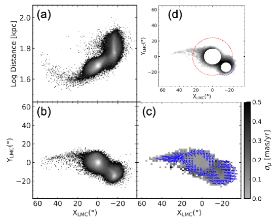
Figure 6: The distribution of modeled MCs in the sky and distance maps. Panel a: particles distance distribution along X_LMC . Panel b: particle distribution in the sky with orthographic projection (see the definination in Gaia Collaboration et al., 2021). Panel c: particle distribution with color indicates proper motion dispersion comparing with $Gaia$ data (Gaia Collaboration et al., 2021), and blue arrows show the proper motion vectors. Panel d: number density distribution of simulation model. The red and blue dashed line indicate the selection region with Gaia EDR3 in Gaia Collaboration et al. (2021).

By using the first year Dark Energy Survey data, Mackey et al. (2016) identified the Northern Tidal Arm (NTA), which emanates from the edge of LMC, and stretches more than 12.5 degree. This feature has been confirmed by further studies (Mackey et al., 2018; Belokurov & Erkal, 2019). The stellar population of the NTA matches well that of LMC, which is predominantly old with $[Fe/H]$ $\sim$ -1. This indicates a LMC origin for the NTA. $Gaia$ EDR3 provides deep astrometric data, and in particular, proper motions may provide important constraints about the NTA origin.

Gaia Collaboration et al. (2021) confirm this NTA feature and found that it stretches to more than 20 degree, with NTA stars showing motions towards the LMC (see their figure 17). To compare with the $Gaia$ data, we project our simulation data (see the panel b of Fig. 6) to the same frame as Gaia Collaboration et al. (2021). Simulations predict a north giant stream starting from the LMC edge, which match well with the NTA, though it stretches a larger angle, $\sim$ 60 degrees.

Since the discovery of NTA, several simulation models have been run to explore the origin of NTA (Mackey et al., 2016; Belokurov & Erkal, 2019; Cullinane et al., 2022a). As pointed out by Gatto et al. (2022) they only produced a more diffuse twisted stream. In the panel d of Fig.6 we show the surface number density distribution of our simulation model. Our model can produce a straight stream that resembles the NTA. The NTA is thin in particular at the tip, but at the edge of LMC the simulated NTA are thick, which are likely associated to other substructures (see discussion in next section).

Panel a of Fig. 6 shows the distance versus the longitude distribution. The simulated NTA shows a gradient in distance, which decreases from the edge of LMC to $\sim 38$ kpc at 30 degree away from the LMC, and then increases to $\sim 56$ kpc at $\sim 55$ degree away from LMC. It confirms that the NTA originates from the LMC. We note that the recent observation from Magellanic Edges Survey (Cullinane et al., 2020, 2022a, MagES) have confirmed an LMC origin for the NTA on the basis of its geometry, metallicity and kinematics.

In the simulation, the interaction between the Clouds triggers instabilities of LMC disk, and then the disturbed LMC disk further suffers the strong Milky Way gravity tidal field that forms a tidal arm and stretches it along when the LMC falls into the MW. This explains well why NTA and LMC stellar population are so similar. The simulation thus predicts that there may be a much longer NTA at lower surface brightnesses, which needs to be confirmed by deeper observations.

3.2 Comparing the morphology of Northern Tidal Arm and North-Eastern structure with observation

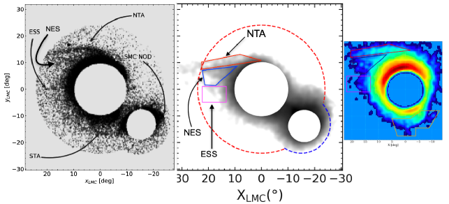
Figure 7: Comparing the morphology of MCs with Gaia EDR3 data. The left panel is from Gaia Collaboration et al. (2021), the middle panel shows the Wang et al. (2019) model, and the right panel is from Gatto et al. (2022) using Gaia EDR3 data with a Gaussian Mixture Model to a sample of strictly selected candidate members of the Magellanic System. In the middle panel, the red and blue dashed-line indicate the sample selection region for Gaia data (Gaia Collaboration et al., 2021). In the right panel, the colored polygon regions indicate different substructures associated with LMC detected by Gatto et al. (2022). The red, blue, and magenta polygon regions on right panel indicate the NTA, North-Eastern structure (NES), and Eastern Substructure (ESS), which are placed on the middle panel with corresponding position.

Fig.7 give a close comparison morphology of substructures in the periphery of LMC. The left panel shows the faint features presented in Gaia Collaboration et al. (2021) with $GAIA$ EDR3, in which the NTA is clearly identified as well as several other substructures indicated by arrows, such as Eastern Substructure (ESS El Youssoufi et al., 2021). Recenly, using a Gaussian Mixture Model to a strictly selected sample of Magellanic System, Gatto et al. (2022) confirmed these substructures, e.g., NTA (red polygon in the right panel of Fig.7) and ESS (magenta rectangle in the right panel of Fig.7). In the meanwhile, they also find a new diffuse sub-structure protruding from the outer LMC disc, which extends to more than 20 degree from the center of LMC. The new feature is named North-Eastern Structure (NES) and indicated by a blue polygon in the right panel of Fig.7.

The middle panel of Fig.7 shows our model, which predicts both the NTA and the NES. Besides these two structures, in the eastern part of LMC there is substructure which could be associated with ESS. In the bottom left panel of Fig.6, there are many particles along the NTA in the eastern of LMC, which have the same origin as NTA and are induced by Galactic tides on the LMC. Therefore, the Wang et al. (2019) reproduces NTA, NES, and ESS. Future observations to measure the metallicity of NES and ESS are needed to compare with NTA and verify their origin.

3.3 The distance to NTA

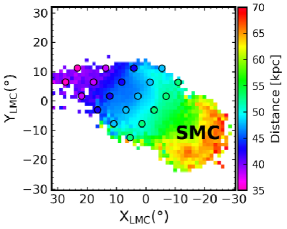
Figure 8: The distribution of the line-of-sight distance for our modelled MCs, and the colored circles show the distances for a disk with inclination $i=34$ degree and orientation of 139.1 degree following van der Marel & Kallivayalil (2014). By examing the distances for a few observed fields associated with NTA with red clump stars, Cullinane et al. (2022a) found that the distance distribution of NTA follow the disk geometry of van der Marel & Kallivayalil (2014) very well within $\sim 20$ degree.

Cullinane et al. (2022a) using data from Magellanic Edges Survey (MagES) (Cullinane et al., 2020) and $Gaia$ EDR3 have studied the kinematic, metallicity and distance for the NTA. Their fields cover to $\sim 20$ degree along NTA. They found that the NTA is near the plane of the LMC disc, with an inclination $i=34$ degree and an orientation $\Omega=139.1$ degrees (van der Marel & Kallivayalil, 2014). Fig.8 shows the line of sight distance for our model, in which colored circles indicate an inclined disc with a geometry following van der Marel & Kallivayalil (2014). Our modeled NTA follows well this inclined disc within $\sim 20$ degree, which is consistent with measurements by Cullinane et al. (2022a).

Fig.8 shows a gradient of distance in our modeled SMC from the eastern to the western part of the SMC, with the western part (see red color on the right) at more far distance than the eastern part (see green color on the left of the SMC). In the observation, there is indeed a distance gradient identified with different tracers. Muraveva et al. (2018) used 2997 RR Lyrae stars to study the three-dimensional structure of SMC. They found that the line-of-sight depth of SMC is in the range 1-10 kpc, and the eastern part of the SMC is located closer to us than that of the western part. Grady, Belokurov & Evans (2021) used Gaia DR2 RR Lyrae to trace the the three-dimensional distribution of MCs, and they arrived to the same conclusion, i.e., the eastern portion of SMC lies at closer distance. Scowcroft et al. (2016) used classical Cepheids to study the three-dimensional structure of the SMC, and they found that the eastern side is up to 20 kpc closer than its western side. The different distance gradient depends on the different stellar populations, which reflects the different morphologies and line-of-sight distributions (Ripepi et al., 2017). Even though detailed comparison of the depth distribution for SMC between observation and our model will require detailed stellar population modeling and sample selection, the Wang et al. model predicts and reproduces the existence of this distance gradient from eastern to western part of SMC.

3.4 The kinematics of NTA

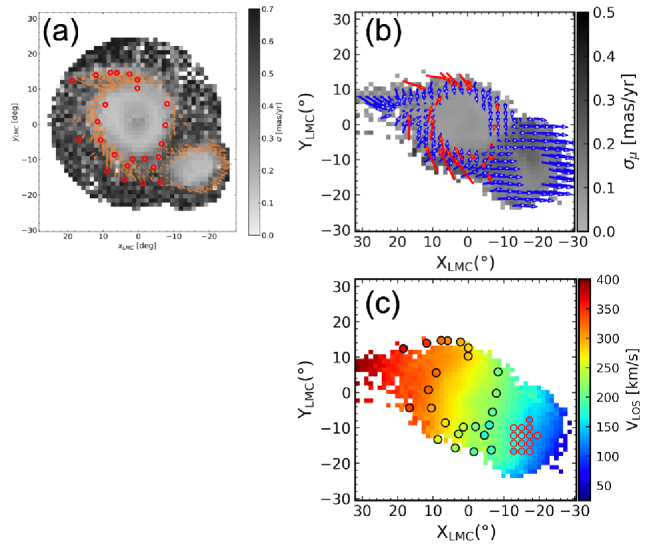
Figure 9: The panel a is from Gaia Collaboration et al. (2021) with $Gaia$ EDR3 showing the proper motion dispersion map and proper motion vectors shown by orange arrows. We note that there is no proper motion vector scale length available from Gaia Collaboration et al. (2021). The red circles indicate the observed fields by MagES (Cullinane et al., 2020). The panel b shows the simulated MCs with blue arrows indicating the modeled proper motions, and the red arrows indicate the proper motions derived from MagES in each observed field. The panel c shows our modeled line-of-sight velocity field, and big colored circles around LMC indicate the line-of-sight velocity from MagES (Cullinane et al., 2022a, b). The small colored circles in the center of the SMC are observed line-of-sight velocities from literature data (see the text for details).

Fig.9 compares the proper motions from Gaia EDR3 data (Gaia Collaboration et al., 2021) (orange arrows in the panel a) with our model (panel b). The proper motions of stars in the simulated NTA (panel b of Fig.9) imply that they are moving towards the LMC, which matches well with $Gaia$ results, except at the location closest of the LMC, for which model deviates from the observations. As in the observations, the dispersion of the proper motions in the simulated NTA are small. The length scale of proper motion vectors are different between model and observations data because of the lack of information about the amplitude of the observed proper motion vector (Gaia Collaboration et al., 2021).

With MagES (Cullinane et al., 2020) combined with Gaia EDR3 data, Cullinane et al. (2022a, b) have selected members of Magellanic Cloulds with fitting a multi-dimensional Gaussian distribution to the LOS velocity and proper motion. There are 26 selected fields observed in the periphery of LMC as indicated by red circles in the panel a of Fig.9. With these data, they have derived the proper motions for each field, which are shown by red arrows in the panel b of Fig.9 for comparison with our modeled proper motion. The proper motion of simulated NTA show downwards motion close to LMC disk, while the observation data show bottom-right toward motion. We note that the four red arrows in the outmost bottom-left disk have very large vector length. This could be due either to a small number of stars available for measurements from MagES, or because they are associated with faint substructures(Cullinane et al., 2022b; El Youssoufi et al., 2021) which are not reproduced by current models.

With MagES, the LOS velocity for each field is also derived from the members stars, which are shown by colored circles in the panel c of Fig.9 for comparison with our modeled line-of-sight velocity map. The simulated LOS velocity field follows well that observed (colored circles).

We note that there is a radial velocity gradient across SMC with increasing radial velocity toward LMC. With new spectroscopic data of $\sim 3000$ RGB and complemented by literature spectroscopic measurement, De Leo et al. (2020) have identified a large scale radial velocity gradient for SMC with increasing velocity toward the Magellanic Bridge (see their Figure 7). To have a better comparison with observations, we have collected observation data of radial velocities in the SMC from literature, including $\sim 3000$ RGB stars from Dobbie et al. (2014), and $\sim 2000$ from Evans & Howarth (2008) with majority of OBA type stars, as well as data from De Leo et al. (2020). These observed radial velocities in the SMC are shown within the small colored circles in the panel c of Fig.9. Even though these observed data are focused on the central SMC, the observed velocity gradient matched well with modeled one, confirming that the Wang et al. (2019) velocity field in SMC follows the observational data.

4 DISCUSSION

Even though the MS has been discovered for about fifty years, there is still no agreement about its origin, which from the literature could be either a gigantic tidal tail, or two ram pressure tails trailing behind each of the two Clouds. Both origins are consistent with the fact that the MS is trailing behind the Clouds (Mathewson, Cleary & Murray, 1974), and that the recent collision between the Clouds had formed the Bridge. However, the tantalizing amount of high precision data provided by $Gaia$ and ground-based surveys that is now available, is probably sufficient to disentangle which mechanisms lead to the MS formation.

In the following, we do not discuss the LA formation, which can be either attributed to the Cloud interaction (Besla et al., 2012; Lucchini et al., 2020), or to dwarfs passing ahead of the Clouds, which have lost their gas at different locations explaining then the LA four arm behavior (Hammer et al., 2015; Wang et al., 2019; Tepper-García et al., 2019; Lucchini, D’Onghia & Fox, 2021). First, this is because forcing the LA to be of the same origin than the MS could lead to misleading results. Second, there are more evidences that the LMC is associated to dwarfs (Patel et al., 2020), and also that many MW dwarfs have a recent infall like the LMC (Hammer et al., 2021), which let plausible a formation of the four leading arms by passages of several leading gas-rich dwarfs.

Table 1 provides a list of the Magellanic System main properties, and describes the ability of four modeling to reproduce them. We have chosen to describe only models based on a first passage of the Clouds, which let us with the tidal models of Besla et al. (2012), Lucchini et al. (2020), and Lucchini, D’Onghia & Fox (2021), and with the ’ram-pressure plus collision’ model of Wang et al. (2019). Here we do not compare the model of Hammer et al. (2015), because the Wang et al. (2019) model is its direct adaptation by just changing the $GADGET2$ by the $GIZMO$ software, for a better accounting of the Kelvin-Helmholtz (KH) instabilities. Such instabilities have to be accounted to constraint the MW halo gas content from the MS actual length and distance, as well as to properly account for the ionized gas kinematically associated to the MS (Fox et al., 2014).

Ionized gas properties cannot be simulated by the Besla et al. (2012) model, since it does not include the MW halo gas, which cannot then interact with the predicted gaseous tidal tail. Because the Besla et al. (2012) model predicts a 10 times smaller HI mass than that observed in the MS is a major problem for this modeling, since adding the MW hot gas corona can only decrease the HI mass due to KH instabilities. However, this problem has been circumvented by Lucchini et al. (2020), who further added a hot corona to the LMC, in order to account for the large ionized gas mass associated to the MS.

In Table 1 we do not account for the mass properties of the remnant Clouds, because these properties can be tuned after modifying their initial conditions. However, the goal is to reproduce the whole MS properties, together with the Cloud orbital motions, for which measurements from $Gaia$ accurately define their orbits and the way they have deposited their gas to form the MS.

Table 1 also shows that the Wang et al. (2019) model reproduces all the main properties of the MS, while other modeling fail for at least half of them. However, as argued by Tepper-García et al. (2019), one may consider that the initial conditions rely on a large number of model-dependent, and thus necessarily tuneable parameters leading to costly numerical experiments, and then prohibitive (or even ’futile’) to explore in full the available parameter space. Following these considerations, one would only conclude that the ’ram-pressure plus collision’ model is just the more advanced one by providing an explanation of all MS properties, but that a tidal model could in principle reach the same success.

However, this paper shows that the ’ram-pressure plus collision’ model does not only reproduce the MS properties, but is also predictive, e.g., for the complex properties of stars in the Bridge, or for the NTA formation. Moreover, one may try to identify properties that cannot be reproduced by the tidal model. To do so, we propose to reinvestigate the physical properties of the MS as reported by Hammer et al. (2015) after their examination of the exquisite data from the Galactic All-Sky Survey (GASS; McClure-Griffiths et al., 2009; Kalberla et al., 2010). It revealed two inter-twisted filaments along the MS length, characterized by a transonic flow (see also Bland-Hawthorn et al. 2007) in a moderate to low turbulent medium (Reynolds parameter, $R_{e}$, of few hundred) . These last properties are consistent with the presence of vortices anchored into the inter-twisted filaments (Hammer et al., 2015).

Perhaps the major drawback of the tidal model is that it cannot reproduce the MS morphology (e.g., the inter-twisted filament behavior), including the fact that kinematic and chemical analyses indicate that gas from both the LMC and SMC is present in the MS, as it is argued by Lucchini et al. (2020). The Lucchini et al. (2020) simulations indeed include an additional filament that seems attached to the LMC as it is observed (Nidever, Majewski & Butler Burton, 2008), but the simulated MS HI morphology is so wide (see their Figure 2) that it show very few similarities with the observed narrow inter-twisted filaments (Hammer et al., 2015, see their Figure 2). The major addition made by Lucchini et al. (2020) to the Besla et al. (2012) model from which it is adapted, is indeed to add a Galactic corona to the MW as well as another corona to the LMC. The advantage of the later addition is to reproduce by construction the large amounts of ionized gas following the MS. However, this is at the cost of predicting a larger mass for the hot corona associated to the LMC than that linked to the MW (3 $\times 10^{9}$$M_{\odot}$ versus 2 $\times 10^{9}$$M_{\odot}$, respectively), which appears unrealistic.

Such a major difficulty has been identified and corrected by Lucchini, D’Onghia & Fox (2021), but at the cost of changing dramatically the Cloud orbits, in such a way that their accurately observed velocities are not reproduced at $\geq$ 3$\sigma$ (and from 7 to 18 $\sigma$) for the LMC (SMC) tangential velocity components, respectively. Figure 10 shows the comparison of the ’ram-pressure plus collision’ model (panel c and d) with observational data (panel a and b), the model is from Wang et al. (2019). In panels c and d, the Leading Arm data from Hammer et al. (2015) have been added assuming the scenario of gas deposited from former runners of several gas-rich dwarfs. The model and observations can be compared with Figure 2 in Lucchini et al. (2020) and Figure 3 in Lucchini, D’Onghia & Fox (2021).

In summary, the ’ram-pressure plus collision’ model succeeds to reproduce all the MS properties and is found to be also predictive, while the tidal model appears unable by construction to reproduce the very well defined inter-twisted filaments that constitute the MS. Moreover, tidal models that may reproduce the associated large amounts of ionized gas have led to inconsistencies either on the relative mass of the LMC vs MW coronas, or on the LMC and SMC tangential velocities.

Figure 10: Comparison of MS in the distribution of Magellanic longitude versus latitude coordinates and longitude versus line-of-sight velocity. Panel (a) and (b) show the observation results from Nidever et al. (2010). The panel (c) and (d) show model results from the ’ram-pressure plus collision’ model (Wang et al., 2019), assuming Leading Arm formation from Hammer et al. (2015) with a scenario of gas deposited from several former leading gas-rich dwarfs. The observations and model can be compared with the panel (d) and (e) of Figure 3 of Lucchini, D’Onghia & Fox (2021), and the panel (b) and (c) of Figure 2 of Lucchini et al. (2020) from tidal model with massive LMC corona.

Table 1: Comparing three modelings for reproducing the main properties of the Magellanic System

	Tidal Model	Ram-pressure+Collision	Tidal+LMC corona	Tidal+LMC corona
Observation Constraints	Besla et al. (2012)	Hammer et al. (2015)	Lucchini et al. (2020)	Lucchini, D’Onghia & Fox (2021)
		Wang et al. (2019)
MS ionized gas mass	N	Y	Y	N
MS ionized gas sky distribution	N	Y	Y	Y
MS HI total mass	N	Y	Y	Y
MS HI gas velocity distribution	Y	Y	N	Y
two inter-twisting filaments	N	Y	N	N
No stars in the MS	N	Y	N	N
Cloud proper motions	Y	Y	Y	N
HI bridge	Y	Y	Y	Y
Young and old stellar bridge	Y	Y	?	?

Table 1 points out the fact that the ”ram-pressure plus collision” model naturally reproduce as much as possible the numerous properties of the Magellanic System. This could be considered as natural, since the LMC HI disk has been undoubtedly shrunk by ram pressure effects (Nidever, 2014), and such a gas is expected to be trailing to form the LMC contribution to the MS. The predictive ability of this model (MB population and NTA) further indicates that this model goes into the right direction to disentangle the mystery of Magellanic System formation (Don Mathewson, 2015, private communication). The only possible ’caveat’ of the ”ram-pressure plus collision” model is that it predicts a moderate LMC mass to let the HI gas being extracted by ram-pressure to form the neutral Stream, especially between the Bridge and the tip-end. Wang et al. (2019) simulations are based on small masses for the LMC, and they mentioned having failed in reproducing the MS for LMC masses larger than 2 $\times 10^{10}$ $M_{\odot}$. In fact, the more massive is the ram-pressurized galaxy, the more difficult is it to extract neutral HI gas (Yang et al., 2022). However, a full numerical study is needed to estimate the highest mass for the LMC halo that would not prevent the formation of the HI Magellanic Stream.

5 CONCLUSION

Here we show that the ’ram-pressure plus collision’ model (Hammer et al., 2015; Wang et al., 2019) is able to reproduce all the MS properties, as well as to predict new features that have been observed after the model elaboration, without fine tuning. The new observation features include the complexity of the stellar populations in the MB and the NTA. The MB is likely caused by the Cloud collision 200-300 Myr ago, for which the LMC has tidally extracted large amounts of gas from the SMC, the MB gas being then affected by the ram pressure exerted by the MW corona. Wang et al. (2019) explained as such the spatial and kinematic behavior of both Young Main Sequence stars and ancient RR Lyrae stars (Belokurov et al., 2017). Besides this, the stellar populations found at two different distances in the MB region by Omkumar et al. (2021) are also predicted by the Wang et al. (2019) model. The model also predicts that the foreground population results from the Cloud tidal interaction (mostly stars extracted from the SMC), while the background population is associated to SMC spheroid stars that have been tidally extracted and reshaped by the LMC. We have also compared proper motions from $Gaia$ EDR3 (Gaia Collaboration et al., 2021) between young stars and the RC old stars in the MB region with Wang et al. (2019) model predictions. Both observations and model show that stars in the Bridge are moving consistently to the LMC. Recent identifications of the NTA and of its kinematics from $Gaia$ EDR3 have been also reproduced by Wang et al. (2019) model, which infers its origin from the LMC tidal stretching by MW tidal force.

The ability of the ’ram-pressure plus collision’ model contrasts with that of the tidal model that essentially fail to reproduce half of the main properties of the MS. In particular, the HI MS is mostly made of two inter-twisted filaments, which tidal models fail to reproduce, and for which no interpretation can be foreseen if the MS is a tidal tail. Moreover, the tidal model has difficulties to reproduce the MS gas mass, especially its dominant phase, the ionized gas, for which the proposed solutions appear either unrealistic, or with strong deviations from the calculated Cloud velocities. It is then likely that the MS is made by ram pressure exerted by the MW corona to the Clouds since their entrance into the halo. This, combined with the 200-300 Myr collision that is robustly determined from the $Gaia$ proper motions of the Clouds, from their common star formation history, and from the Bridge, suffices to explain the whole MS properties. We further conjecture that to form the Magellanic Stream, the LMC mass has to be smaller than 2 $\times 10^{10}$ $M_{\odot}$, though further studies are needed to precise the exact mass range.

DATA AVAILABILITY

The data underlying this article will be shared on reasonable request to the corresponding author.

Appendix A Gaussian fitting to the distance distribution

Two Gaussian function are used to fit the distance distribution of particles within different MB longitude bins as shown in Figure 11.

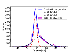
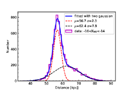
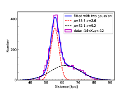
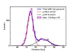
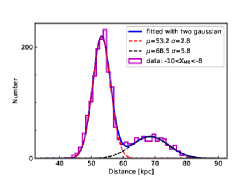
Figure 11: Distances distributions for particles (magenta) within different MB longitudes intervals. Two Gaussian functions are used to fit the distance distributions for foreground (red-dashed line) and background (black-dashed line) population, with their mean and standard deviation are labeled on the top right of each panel. The blue-solid line indicate the sum of two Gaussian functions.

References

- Bagheri, Cioni & Napiwotzki (2013) Bagheri G., Cioni M.-R. L., Napiwotzki R., 2013, A&A, 551, A78
- Belokurov et al. (2017) Belokurov V., Erkal D., Deason A. J., Koposov S. E., De Angeli F., Evans D. W., Fraternali F., Mackey D., 2017, MNRAS, 466, 4711
- Belokurov & Erkal (2019) Belokurov V. A., Erkal D., 2019, MNRAS, 482, L9
- Besla, Hernquist & Loeb (2013) Besla G., Hernquist L., Loeb A., 2013, MNRAS, 428, 2342
- Besla et al. (2007) Besla G., Kallivayalil N., Hernquist L., Robertson B., Cox T. J., van der Marel R. P., Alcock C., 2007, ApJ, 668, 949
- Besla et al. (2012) Besla G., Kallivayalil N., Hernquist L., van der Marel R. P., Cox T. J., Kereš D., 2012, MNRAS, 421, 2109
- Bland-Hawthorn et al. (2007) Bland-Hawthorn J., Sutherland R., Agertz O., Moore B., 2007, ApJ Lett., 670, L109
- Bregman et al. (2018) Bregman J. N., Anderson M. E., Miller M. J., Hodges-Kluck E., Dai X., Li J.-T., Li Y., Qu Z., 2018, ApJ, 862, 3
- Casetti-Dinescu et al. (2012) Casetti-Dinescu D. I., Vieira K., Girard T. M., van Altena W. F., 2012, ApJ, 753, 123
- Conroy et al. (2021) Conroy C., Naidu R. P., Garavito-Camargo N., Besla G., Zaritsky D., Bonaca A., Johnson B. D., 2021, Natur, 592, 534
- Cullinane et al. (2022a) Cullinane L. R., Mackey A. D., Da Costa G. S., Erkal D., Koposov S. E., Belokurov V., 2022a, MNRAS, 510, 445
- Cullinane et al. (2022b) Cullinane L. R., Mackey A. D., Da Costa G. S., Erkal D., Koposov S. E., Belokurov V., 2022b, MNRAS, 512, 4798
- Cullinane et al. (2020) Cullinane L. R. et al., 2020, MNRAS, 497, 3055
- De Leo et al. (2020) De Leo M., Carrera R., Noël N. E. D., Read J. I., Erkal D., Gallart C., 2020, MNRAS, 495, 98
- Dehnen (1993) Dehnen W., 1993, MNRAS, 265, 250
- Demers & Battinelli (1998) Demers S., Battinelli P., 1998, AJ, 115, 154
- Dobbie et al. (2014) Dobbie P. D., Cole A. A., Subramaniam A., Keller S., 2014, MNRAS, 442, 1663
- El Youssoufi et al. (2021) El Youssoufi D. et al., 2021, MNRAS, 505, 2020
- Erkal et al. (2019) Erkal D. et al., 2019, MNRAS, 487, 2685
- Erkal et al. (2021) Erkal D. et al., 2021, MNRAS, 506, 2677
- Evans & Howarth (2008) Evans C. J., Howarth I. D., 2008, MNRAS, 386, 826
- Faerman, Sternberg & McKee (2017) Faerman Y., Sternberg A., McKee C. F., 2017, ApJ, 835, 52
- Fox et al. (2014) Fox A. J. et al., 2014, ApJ, 787, 147