Unsupervised Deep Discriminant Analysis Based Clustering

Abstract

This work presents an unsupervised deep discriminant analysis for clustering. The method is based on deep neural networks and aims to minimize the intra-cluster discrepancy and maximize the inter-cluster discrepancy in an unsupervised manner. The method is able to project the data into a nonlinear low-dimensional latent space with compact and distinct distribution patterns such that the data clusters can be effectively identified. We further provide an extension of the method such that available graph information can be effectively exploited to improve the clustering performance. Extensive numerical results on image and non-image data with or without graph information demonstrate the effectiveness of the proposed methods.

1 Introduction

Clustering, which aims to aggregate similar data together and separate dissimilar data, is a fundamental yet challenging research problem in machine learning and data mining (Jain, 2010). Classicial clustering methods such as k-means clustering (Hartigan and Wong, 1979), spectral clustering (Shi and Malik, 2000; Ng et al., 2001), and subspace clustering (Vidal, 2011; Liu et al., 2013; Matsushima and Brbic, 2019; Fan, 2021) have been well studied but their performance are not satisfactory when the structures of data are quite complex or the features are not discriminative. Recently, many researchers (Xie et al., 2016; Yang et al., 2016; Jiang et al., 2017; Ji et al., 2017; Ghasedi Dizaji et al., 2017; Abavisani et al., 2020; Tang et al., 2020; Lv et al., 2021; Zhang and Davidson, 2021; Peng et al., 2022) focus on improving classical clustering methods by exploiting the strengths of deep learning such as auto-encoder (AE) (Hinton and Salakhutdinov, 2006) in data representation. For instance,  Xie et al. (2016) proposed a deep embedded clustering (DEC) method via integrating feature learning and clustering in a unified network. Ji et al. (2017) proposed a deep subspace clustering method based on AE and self-expression (Elhamifar and Vidal, 2013). Note that those self-expression based deep clustering methods such as (Ji et al., 2017; Zhang and Davidson, 2021) have at least quadratic time and space complexity and hence are not applicable to very large datasets (Matsushima and Brbic, 2019; Fan, 2021).

More recently, a few researchers (Zhao et al., 2021; Zhang et al., 2020; Tu et al., 2021) proposed to integrate graph convolutional networks (Kipf and Welling, 2017; Veličković et al., 2018) into deep clustering methods such that both Euclidean feature and graph structure can be utilized for clustering. For instance, Bo et al. (2020) proposed a structural deep clustering network (SDCN), which uses GCN module to provide graph structure information among data in the clustering-oriented embedding learning. Peng et al. (2021) proposed an attention graph clustering network (AGCN), which improves SDCN by introducing an attention mechanism to dynamically fuse the embedded representation and graph feature, as well as the representations learned by different GCN layers. In these methods, it is expected that exploiting more useful information can improve the clustering performance.

The aforementioned deep clustering methods do not explicitly ensure distinct and compact cluster structures, which may lead to difficulties in partitioning data points around decision boundaries. An intuitive example is shown by Figure 5 (also Figure 2 in the supplement). In this paper, we propose a novel clustering method called deep discriminative analysis based clustering (DDAC). Specifically, we use an autoencoder to learn the embedded representation for the input data and propose to minimize the intra-cluster discrepancy and maximize the inter-cluster discrepancy of the data representation to pursue more discriminative and compact latent representation. We also provide an extension of DDAC that is able to effectively exploit the graph information for clustering. Our contributions are as follows.

• We present a novel unsupervised deep discriminant analysis based clustering method, which extends linear discriminative analysis to unsupervised deep learning.

• We propose an effective regularizer to obtain small intra-cluster discrepancy and large inter-cluster discrepancy in the data. To ensure unsupervised discriminative projection, we provide a dynamic confidence assignment mechanism to increase the reliability of the intra-cluster discrepancy.

• We further extend our method to graph based clustering. It enables us to take advantages of both feature information and graph information to do clustering in an unsupervised deep discriminative manner.

Empirical studies on many benchmark datasets show that our methods can outperform the baselines.

2 Deep Discriminant Analysis Based Clustering (DDAC)

Suppose we have a data matrix $\mathbf{X}\in\mathbb{R}^{n\times d}$, where $n$ denotes the number of samples and $d$ denotes the number of features or variables. Our goal is to cluster the rows of $\mathbf{X}$ into $k$ groups. We consider the case that the variables of $\mathbf{X}$ are not discriminative such that classical clustering methods such as k-means, spectral clustering, and subspace clustering are not effective in identifying the clusters. Therefore, instead of directly clustering the rows of $\mathbf{X}$, we want to extract some discriminative features denoted by $\mathbf{Z}=[\mathbf{z}_{1},\mathbf{z}_{2},\ldots\mathbf{z}_{n}]^{\top}\in\mathbb{R}^{n\times d^{\prime}}$ from $\mathbf{X}$ and then cluster the rows of $\mathbf{Z}$. Specifically, we use a feature extractor $h_{\theta}$ to get

$$\mathbf{z}_{i}=h_{\theta}(\mathbf{x}_{i}),\quad i=1,2,\ldots,n,$$ (1)

where $\theta$ denotes the set of parameters that can be learned from $\mathbf{X}$. Suppose we have already known the labels of the columns of $\mathbf{Z}$. Then we define an intra-cluster discrepancy as

$$D_{\text{intra}}:=\frac{1}{n}{\sum_{j=1}^{k}\sum_{i\in c_{j}}\left\|\textbf{z}_{i}-{\bm{\mu}_{j}}\right\|^{2}},$$ (2)

where $\bm{\mu}_{j}=\frac{1}{|c_{j}|}\sum_{i\in c_{j}}\mathbf{z}_{i}$ is the centroid of cluster $j$ and $c_{j}$ denotes the set of indices of data points in cluster $j$. Besides, we also define an inter-cluster discrepancy as

$$D_{\text{inter}}:=\sum_{j=1}^{k}\sum_{m=1}^{k}\left\|\bm{\mu}_{j}-\bm{\mu}_{m}\right\|^{2}.$$ (3)

We say that $\mathbf{Z}$ is discriminative if

$$\mathcal{L}_{\textrm{disc}}:={D_{\text{intra}}}/{D_{\text{inter}}}$$ (4)

is large. We hope to learn a $h_{\theta}$ to maximize $\mathcal{L}_{\textrm{disc}}$ as much as possible. This is similar to the idea of Fisher linear discriminative analysis (LDA) (Bishop and Nasrabadi, 2006) that aims to learn a linear projection to maximize the between-class variance and minimize the within-class variance.

However, our goal is clustering and hence the labels of $\mathbf{Z}$ are unknown. First, we need to ensure that $\mathbf{Z}$ should preserve as much information of $\mathbf{X}$ as possible. Therefore, we propose to use an encoder-decoder model to obtain $\mathbf{Z}$, i.e., minimizing

$$\mathcal{L}_{\text{recon}}:= \frac{1}{2n}\sum_{i=1}^{n}\left\|\mathbf{x}_{i}-f_{\theta^{\prime}}({\mathbf{z}_{i}})\right\|^{2}=\frac{1}{2n}\sum_{i=1}^{n}\left\|\mathbf{x}_{i}-f_{\theta^{\prime}}({h_{\theta}(\mathbf{x}_{i})})\right\|^{2},$$ (5)

where $f_{\theta^{\prime}}(\cdot)$ denotes the decoder with parameters set $\theta^{\prime}$. Both $h_{\theta}$ and $f_{\theta^{\prime}}$ are neural networks.

Now we propose to estimate the labels of $\mathbf{Z}$ iteratively. Specifically, following the definition in  (Van Der Maaten and Hinton, 2008; Xie et al., 2016), we define a matrix $\mathbf{Q}\in\mathbb{R}^{n\times k}$ as

$$q_{ij}=\frac{(1+\left\|\mathbf{z}_{i}-\bm{\mu}_{j}\right\|^{2})^{-1}}{\sum_{j^{\prime}=1}^{k}(1+\left\|\mathbf{z}_{i}-\bm{\mu}_{j^{\prime}}\right\|^{2})^{-1}},\quad i=1,\ldots,n,~{}j=1,\ldots,k,$$ (6)

where ${\bm{\mu}}_{j}$ denotes the $j$-th cluster centroid and is initialized by $k$-means performed on a temporary $\mathbf{Z}$. $q_{ij}$ denotes the probability that allocates sample $i$ to cluster $j$. Therefore, $\mathbf{Q}$ is a soft label matrix but can be far from the true label matrix. Similar to (Xie et al., 2016), we introduce a reinforced soft label matrix $\mathbf{P}$ by

$$p_{ij}=\frac{q_{ij}^{2}/\sum_{i=1}^{n}q_{ij}}{\sum_{j^{\prime}=1}^{k}q_{ij^{\prime}}^{2}/\sum_{i=1}^{n}q_{ij^{\prime}}},\quad i=1,\ldots,n,~{}j=1,\ldots,k.$$ (7)

$\mathbf{P}$ should be sparser than $\mathbf{Q}$ and the very large or very small values in $\mathbf{P}$ are more reliable than those in $\mathbf{Q}$ as soft labels. Nevertheless, $\mathbf{P}$ or $\mathbf{Q}$ cannot be directly used to generate labels for $\mathbf{Z}$ when considering (2). The reason is that the probabilities given by (6) are just estimations of the clustering tendency and the unreliable probabilities can lead to unreliable discriminative latent representation. Therefore, we design a confident assignment selection mechanism to mitigate the negative effects of unreliable probabilities. It is mathematically formulated as an indicator vector $\mathbf{t}\in\mathbb{R}^{n}$ defined by

$$t_{i}=\left\{\begin{matrix}1,&\max_{1\leq j\leq k}(p_{ij})>\delta,\\ 0,&\mbox{ otherwise. }\end{matrix}\right.$$ (8)

Here $\delta$ denotes a global threshold above which the clustering probability for each sample is confident.

Now based on (2), (7), and (8), we can define a reliable estimate of the intra-cluster discrepancy as

$$\hat{D}_{\textrm{intra}}:=\frac{\sum_{j=1}^{k}\sum_{i=1}^{n}\left\|\textbf{z}_{i}-\bm{\mu}_{j}\right\|^{2}\times p_{ij}\times t_{i}}{\sum_{i=1}^{n}t_{i}}.$$ (9)

An estimate of the inter-cluster discrepancy is given by $\hat{D}_{\textrm{inter}}:=\sum_{j=1}^{k}\sum_{m=1}^{k}\left\|\bm{\mu}_{m}-\bm{\mu}_{j}\right\|^{2}={D}_{\textrm{inter}}$. Now we minimize

$$\displaystyle\mathcal{L}_{\textrm{disc}}:=\frac{\hat{D}_{\textrm{intra}}}{\hat{D}_{\textrm{inter}}}=\frac{\sum_{j=1}^{k}\sum_{i=1}^{n}\left\|\textbf{z}_{i}-\bm{\mu}_{j}\right\|^{2}\times p_{ij}\times t_{i}}{(\sum_{i=1}^{n}t_{i})\times\sum_{j=1}^{k}\sum_{m=1}^{k}\left\|\bm{\mu}_{m}-\bm{\mu}_{j}\right\|^{2}}$$ (10)

to obtain a reliable discriminative representation.

Note that in LDA, the variables in the latent space are uncorrelated because the projection vectors are orthogonal. The uncorrelated features are more useful than correlated features. Hence, in our method, we propose to make the columns of $\mathbf{Z}$ orthogonal via considering the following regularization term

$$\mathcal{L}_{\textrm{orth}}:=\frac{1}{\sum_{i=1}^{n}t_{i}}\left\|\hat{\mathbf{Z}}^{\top}\hat{\mathbf{Z}}\odot(\mathbf{O-\hat{\mathbf{I}}})\right\|_{F}^{2},$$ (11)

where $\odot$ denotes Hadamard product, $\hat{\mathbf{Z}}=\mathbf{Z}\odot\mathbf{1}^{\top}\mathbf{t}$ is the selective representation from the confident assignment. $\mathbf{O}\in\mathbb{R}^{d^{\prime}\times d^{\prime}}$ is a matrix with all elements are 1 and $\hat{\mathbf{I}}\in\mathbb{R}^{d^{\prime}\times d^{\prime}}$ is an identity matrix.

In addition, let $\Omega$ be the index set of samples satisfying the condition of confident assignment selection and we want $\mathbf{Q}_{\Omega}$ to be close to $\mathbf{P}_{\Omega}$ via minimizing

$$\mathcal{L}_{\textrm{clus}} :=KL(\mathbf{P}_{\Omega}\left|\right|\mathbf{Q}_{\Omega})=\sum_{i\in\Omega}\sum_{j=1}^{k}p_{ij}\log\frac{p_{ij}}{q_{ij}}=\sum_{i=1}^{n}t_{i}\sum_{j=1}^{k}p_{ij}\log\frac{p_{ij}}{q_{ij}}.$$ (12)

Finally, we have an overall objective function

$$\mathcal{L}(\Theta,\left\{\bm{\mu}\right\}):=\mathcal{L}_{\textrm{recon}}+\alpha\mathcal{L}_{\textrm{clus}}+\beta\mathcal{L}_{\textrm{disc}}+\gamma\mathcal{L}_{\textrm{orth}},$$ (13)

where $\Theta=\left\{\theta,\theta^{\prime}\right\}$ and $\left\{\bm{\mu}\right\}=\left\{\bm{\mu}_{1},\cdots,\bm{\mu}_{k}\right\}$ are the network parameters and cluster centroids respectively. $\alpha$, $\beta$ and $\gamma$ are hyper-parameters.

We summarize the roles of all terms of (13) as follows:

• $\mathcal{L}_{\textrm{recon}}$ aims to preserve the inherent structure of the input data.

• $\mathcal{L}_{\textrm{clus}}$ ensures the network to learn clustering assignment from the embedded representation $\mathbf{Z}$ of the input data.

• $\mathcal{L}_{\textrm{disc}}$ tries to minimize of intra-cluster discrepancy and maximize the inter-cluster discrepancy in the latent space, thereby making the learned representation more discriminative.

• $\mathcal{L}_{\textrm{orth}}$ aims to make the columns of $\mathbf{Z}$ orthogonal so as to obtain uncorrelated latent features.

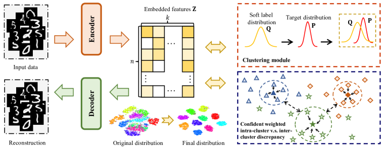
Figure 1: The network architecture of the proposed DDAC method. The input data is first encoded into a low-dimensional embedding features $\mathbf{Z}$ and then $\mathbf{Z}$ is decoded to reconstruct the input data. In the embedding layer, a clustering module is introduced to produce cluster label assignment with $\mathbf{Z}$. Meanwhile, we propose to minimize the intra-cluster discrepancy and maximize the inter-cluster discrepancy of the data representation to pursue discriminative and compact latent representation.

Figure 1 shows the network architecture of the proposed method. The training procedure of the proposed method is illustrated in Algorithm 1, where the final cluster labels are obtained from the soft label distribution $\mathbf{Q}$.

Algorithm 1 Deep Discriminative Analysis Based Clustering (DDAC)

Input: Data matrix $\mathbf{X}$, dimension of latent space $d^{\prime}$, number of clusters $k$, hyper-parameters $\alpha$, $\beta$ and $\gamma$, threshold of confident assignment $\delta$, total training iterations $T$.
Output: Cluster labels $C$.

1:  Initialize $\Theta$, pretrain the autoencoder, and get $\mathbf{Z}$

2:  Initialize the cluster centroids $\{\bm{\mu}\}$ with $k$-means on $\mathbf{Z}$

3:  for $iter=1$ to $T$ do

4:     Compute the soft label distribution $\mathbf{Q}$ using Eq. (6)

5:     Compute the target distribution $\mathbf{P}$ using Eq. (7)

6:     Obtain the selective index set $\mathbf{t}$ using Eq. (8)

7:     Calculate $\mathcal{L}_{\textrm{recon}}$, $\mathcal{L}_{\textrm{clus}}$, $\mathcal{L}_{\textrm{disc}}$, and $\mathcal{L}_{\textrm{orth}}$ using Eqs. (5), (12), (10), and (11) respectively

8:     Update $\Theta$ and $\left\{\bm{\mu}\right\}$ by minimizing Eq. (13) with some optimizer and get $\mathbf{Z}$

9:  end for

10:  Obtain the final clustering results as $c_{i}=\mathop{\arg\max}_{j}~{}q_{ij}$

11:  return  $C$.

3 DDAC with Graph Information

Suppose besides the data matrix $\mathbf{X}\in\mathbb{R}^{n\times d}$, we also have an associated (undirected) graph $G=(V,E)$, in which $V=\{1,2,\ldots,n\}$ denotes the set of vertices corresponding to the data points of $\mathbf{X}$ and $E=\{e_{ij}\}$ denotes the (possibly weighted) edges between the data points. Or equivalently, we can replaced $E$ by an adjacency matrix $\mathbf{A}\in\mathbb{R}^{n\times n}$, in which ${a}_{ij}$ denotes the similarity between vertex $i$ and vertex $j$. Our goal is to cluster the rows of $\mathbf{X}$ or partition the nodes of $G$ into $k$ groups. Note that if $\mathbf{A}$ is not given, we can generate it from $\mathbf{X}$ via some approaches such as $k$ nearest neighbors ($k$NN).

In this section, we propose an extension of DDAC to take advantages of the graph structure. To this end, we incorporate GCN (Kipf and Welling, 2017) into our DDAC to facilitate clustering, yielding a method called DDAC-G. The network architecture of DDAC-G is presented in Appendix A.2 due to the limitation of paper length. For a GCN module with $L$ layers, we can formulate the learned latent features $\mathbf{S}_{l}$ in the $l$-th layer as:

$$\mathbf{S}_{l}=\sigma(\tilde{\mathbf{D}}^{-\frac{1}{2}}\tilde{\mathbf{A}}\tilde{\mathbf{D}}^{-\frac{1}{2}}\tilde{\mathbf{S}}_{l-1}\mathbf{W}_{l}),$$ (14)

where $\mathbf{W}_{l}$ is the weight matrix of the $l$-th layer of the GCN and $\sigma(\cdot)$ denotes the activation function (e.g. ReLU). $\tilde{\mathbf{A}}=\mathbf{A}+\mathbf{I}$, where $\mathbf{I}\in\mathbb{R}^{n\times n}$ is an identity matrix. $\tilde{\mathbf{D}}$ is the degree matrix of $\tilde{\mathbf{A}}$. In order to integrate both the representations learned by AE and GCN, we let $\tilde{\mathbf{S}}_{l-1}=(1-\epsilon)\mathbf{S}_{l-1}+\epsilon\mathbf{Z}_{l-1}$, where $\epsilon$ is fixed as 0.5. Particularly, the input of the first layer of GCN is the original data $\mathbf{X}$, i.e.,

$$\mathbf{S}_{1}=\sigma(\tilde{\mathbf{D}}^{-\frac{1}{2}}\tilde{\mathbf{A}}\tilde{\mathbf{D}}^{-\frac{1}{2}}\mathbf{X}\mathbf{W}_{1}).$$ (15)

The last layer of the GCN utilizes the softmax function to obtain a probability distribution matrix $\mathbf{Y}$ for the categorization of the input data:

$$\mathbf{Y}=\textrm{softmax}(\tilde{\mathbf{D}}^{-\frac{1}{2}}\tilde{\mathbf{A}}\tilde{\mathbf{D}}^{-\frac{1}{2}}\mathbf{S}_{L-1}\mathbf{W}_{L}),$$ (16)

where $y_{ij}$ represents the probability that the GCN network predicts a sample $i$ into cluster $j$. Consequently, by considering both the predictive distribution of AE and GCN, the clustering loss of the DDAC-G method is

$$\mathcal{L}_{\textrm{g-clus}} :=\alpha_{1}KL(\mathbf{P}_{\Omega}\left|\right|\mathbf{Q}_{\Omega})+\alpha_{2}KL(\mathbf{P}_{\Omega}\left|\right|\mathbf{Y}_{\Omega})$$

$$=\alpha_{1}\sum_{i\in\Omega}\sum_{j=1}^{k}p_{ij}\log\frac{p_{ij}}{q_{ij}}+\alpha_{2}\sum_{i\in\Omega}\sum_{j=1}^{k}p_{ij}\log\frac{p_{ij}}{y_{ij}}$$

$$=\alpha_{1}\sum_{i=1}^{n}t_{i}\sum_{j=1}^{k}p_{ij}\log\frac{p_{ij}}{q_{ij}}+\alpha_{2}\sum_{i=1}^{n}t_{i}\sum_{j=1}^{k}p_{ij}\log\frac{p_{ij}}{y_{ij}},$$ (17)

where $\Omega$ denotes the index set of samples that satisfy the condition of confident assignment selection. $\alpha_{1}$ and $\alpha_{2}$ control weights of the two modules and are set to 0.1 and 0.01 respectively in this paper.

Now, based on (5), (10), (11) and (3), the overall objective function of the DDAC-G method is given as

$$\mathcal{L}(\Theta,\left\{\bm{\mu}\right\},\mathcal{W}):=\mathcal{L}_{\textrm{recon}}+\mathcal{L}_{\textrm{g-clus}}+\beta\mathcal{L}_{\textrm{disc}}+\gamma\mathcal{L}_{\textrm{orth}},$$ (18)

where $\Theta=\left\{\theta,\theta^{\prime}\right\}$, $\left\{\bm{\mu}\right\}=\left\{\bm{\mu}_{1},\cdots,\bm{\mu}_{k}\right\}$, and $\mathcal{W}={\left\{\mathbf{W}_{1},\cdots,\mathbf{W}_{L}\right\}}$ are the AE parameters, cluster centroids, and GCN parameters, respectively. $\beta$ and $\gamma$ are two hyper-parameters. It is worth noting that we integrate the learned features in each layer of GCN and AE to obtain more informative features, i.e., $\tilde{\mathbf{S}}$, as the input to the subsequent layer of GCN. Therefore, it makes sense to use the GCN prediction $\mathbf{Y}$ rather than $\mathbf{Q}$ to obtain the cluster assignment. Specifically, $c_{i}=\mathop{\arg\max}_{j}~{}y_{ij}$.

4 Connection with previous work

The main idea of DDAC and DDAC-G is motivated from LDA (Bishop and Nasrabadi, 2006). However, LDA is a supervised learning method and requires reliable labels, which are difficult to obtain in unsupervised scenarios especially when we are using the latent representations of deep neural networks. Therefore, it is non-trivial to extend LDA to deep learning and clustering.

Note that Ding and Li (2007) proposed to perform $k$-means and LDA alternately, which showed much better clustering performance compared to vanilla $k$-means. Ye et al. (2007) showed that the LDA projection can be factored out from the integrated LDA subspace selection and clustering formulation and proposed an algorithm called discriminative k-means for simultaneous LDA subspace selection and clustering. Shaol et al. (2018) introduced a discriminative loss to deep clustering. The discriminative loss can be regarded as a graph regularization for the latent representations, where the similarities are the predicted probability of softmax functions. However, the clustering accuracy (Table I in (Shaol et al., 2018)) of the method is not high compared to the baselines used in our paper. Tzoreff et al. (2018) proposed to obtain discriminative latent space in the pre-training (AE) phase, where the discriminative information are from k-nearest neighbors of data space. The clustering accuracy (Table 2 in (Tzoreff et al., 2018)) is lower than our method (Table 1 in our paper). Chang et al. (2019) proposed a method called deep discriminative clustering that models the clustering task by investigating relationships between patterns with a deep neural network. They introduced a global constraint to adaptively estimate the relationships, and a local constraint based on cluster indicators to learn high-level discriminative representations. The strategy of pursuing discriminative features is different from ours.

5 Experiments on data without graph information

5.1 Experimental settings

We demonstrate the effectiveness of the proposed DDAC in comparison to sixteen baselines (including more than ten strong competitors) on two benchmark datasets MNIST and Fashion-MNIST, which both have 70,000 images of size $28\times 28$ belonging to 10 classes.

In our DDAC, for both datasets, we set $\alpha=0.1$ and choose Adam (Kingma and Ba, 2015) as the optimizer, where the learning rate is 0.001. Since the two datasets are image datasets, we construct our DDAC with fully connected network (FCN) and convolutional neural network (CNN), yielding two methods DDAC-FCN and DDAC-CNN. Specifically, for DDAC-FCN, we use a $d$-500-500-1000-$d^{\prime}$ fully-connected encoder and a symmetric decoder on MNIST and the $d$-500-500-2000-$d^{\prime}$ ones on Fashion-MNIST, where $d^{\prime}$ is set to 10. For DDAC-CNN, we uniformly use $3\times 3$ kernel and convolutional auto-encoder whose encoder and decoder consist of four convolutional layers and two linear layers respectively. The more detailed settings of the network architectures are described in Appendix A.2 of the supplementary material. We first pre-train an auto-encoder with the same network structure as our method for 50 epochs of batch-size 512, and initialize the cluster centroids with $k$-means of 20 runs. Then we train our methods for 200 epochs to obtain the cluster assignment. We use three popular metrics including Clustering Accuracy (ACC), Normalized Mutual Information (NMI), and Adjusted Rand Index (ARI) to evaluate the clustering performance.

5.2 Comparative results

We report the clustering results in terms of three evaluation metrics in Table 1. We see that the proposed methods DDAC-FCN and DDAC-CNN outperform other methods in most cases. It is worth noting that the effectiveness of the proposed discriminative regularizer is demonstrated when we compare DDAC-FCN with DEC and IDEC. The superiority of DDAC-FCN over DEC and IDEC stems from the fact that the large intra-cluster discrepancy and small inter-cluster discrepancy provided by DDAC makes the learned representations more discriminative. Moreover, compared to several state-of-the-art methods, DDAC-FCN and DDAC-CNN also show competitive performance. For instance, in comparison to the second best results (e.g. SENet, NCSC and DEPICT), DDAC-CNN achieves 1.30%, 3.07%, 2.62% improvement in ACC, NMI and ARI on MNIST, as well as 1.66% improvement in NMI on Fashion-MNIST compared to the second best results.

Table 1: Clustering performance on MNIST and Fashion-MNIST. The best three results are highlighted in bold. $h_{\max}$ denotes the size of the largest hidden layer of neural network. $h^{\prime}$ denotes the size of the layer connected with the largest hidden layer of neural network. $d$ denotes the dimension of the data or the latent representation. $\omega$, $F$, and $\kappa$ denote the feature map size, kernel size, and channel number of CNN respectively.

Methods/Datasets	MNIST			Fashion-MNIST			Time
	ACC	NMI	ARI	ACC	NMI	ARI	Complexity
$k$-means (MacQueen and others, 1967)	54.10	50.70	36.70	50.50	57.80	40.30	$O(nk)$
SC (Ng et al., 2001)	69.60	66.30	52.10	50.80	57.50	–	$O(n^{2}k)$
AE (Hinton and Salakhutdinov, 2006)	78.53	74.90	71.64	56.72	55.35	41.29	$O(nh_{max}h^{\prime})$
DEC (Xie et al., 2016)	86.53	83.69	80.29	57.81	62.83	45.71	$O(nh_{max}h^{\prime}+ndk)$
JULE (Yang et al., 2016)	96.40	91.30	92.70	56.30	60.80	39.60	/
DCN (Yang et al., 2017)	85.47	81.73	76.26	53.87	58.84	40.84	/
IDEC (Guo et al., 2017)	88.01	86.38	83.25	57.64	60.13	44.09	$O(nh_{max}h^{\prime}+ndk)$
VaDE  (Jiang et al., 2017)	94.50	87.60	91.30	55.20	57.30	42.30	$O(nh_{max}h^{\prime}+ndk)$
DEPICT (Ghasedi Dizaji et al., 2017)	96.50	91.70	93.20	39.20	39.20	30.40	/
ClusterGAN (Mukherjee et al., 2019)	95.00	89.00	89.00	63.00	64.00	50.00	/
ASPC(w/o DA) (Guo et al., 2019)	93.10	88.60	–	59.10	65.40	–	/
NCSC (Zhang et al., 2019)	94.09	86.12	87.52	72.14	68.60	59.17	$O(dn^{2})$
DFCM (Feng et al., 2020)	88.17	86.54	83.37	62.29	64.54	48.65	/
$k$-DAE (Opochinsky et al., 2020)	88.00	86.00	82.00	60.00	65.00	48.00	$O(kh_{\max}h^{\prime}n)$
SENet (Zhang et al., 2021)	96.80	91.80	93.10	69.70	66.30	55.60	$O(d\rho n^{2})$, $0<\rho<1$
TELL (Peng et al., 2022)	95.16	88.83	89.66	52.66	62.05	43.35	/
DDAC-FCN	97.12	92.86	93.74	67.52	69.08	55.36	$O(nh_{\max}h^{\prime}+ndk)$
DDAC-CNN	98.10	94.87	95.82	68.69	70.26	57.39	$O(\omega^{2}F^{2}\kappa n+ndk)$

It should be pointed out that although some subspace clustering methods such as NCSC and SENet have good clustering performance, they have quadratic (in terms of the number of data points) time and space complexities and hence do not scale to large datasets. In contrast, our DDAC methods have linear time and space complexities and are applicable to very large datasets. For completeness, we show the time complexities of some baselines in Table 1.

We further use t-SNE (Van Der Maaten and Hinton, 2008) to provide a visual comparison of clustering performance. Shown in Figure 2, on MNIST, our methods (DDAC-FCN and DDAC-CNN) have much more compact inter-class structures and distinct inter-class discrepancy than DEC and IDEC. Although clustering on Fashion-MNIST is difficult, our methods still significantly outperform DEC and IDEC visually. By the way, DDAC-CNN performs better than DDAC-FCN in this study.

Figure 2: The comparison of different methods on the t-SNE visualization of the learned representations. The first row is the visualization for MNIST, and the second row is for Fashion-MNIST.

6 Experiments on data with graph information

6.1 Experimental settings

We evaluate the proposed method DDAC-G on clustering data with graph information. We consider three non-graph datasets (USPS, REUTERS-10K, HHAR) and three graph datasets (DBLP, CITESEER, and ACM), which are detailed in Table 2. Note that for the non-graph datasets, we use $k$NN to construct graphs. More details about $k$ and its influence on clustering performance are shown in Appendix A.4 of the supplementary material.

Table 2: Details of the six benchmark datasets (including three non-graph datasets and three graph datasets) in graph clustering experiments.

Dataset name	Type	# Total samples	# Classes	# Dimension
USPS	Image	9,298	10	256
HHAR	Record	10,299	6	561
REUTERS-10K	Text	10,000	4	2,000
ACM	Graph	3,025	3	1,870
DBLP	Graph	4,058	4	334
CITESEER	Graph	3,327	6	3,703

For fair comparison, we follow the settings in (Bo et al., 2020) to construct our model with a $d$-500-500-2000-$d^{\prime}$ fully-connected encoder, the same size for GCN, and a symmetric decoder. The dimension of the latent layer $d^{\prime}$ is fixed as 10. We first pre-train an auto-encoder network for 30 epochs without GCN to initialize the model, then train the model for at least 200 epochs until it meets convergence. The learning rate is set to 1e-3 for USPS, HHAR, and ACM, 2e-4 for REUTERS, and 1e-4 for DBLP and CITESEER. We also conduct ablation study in Appendix LABEL:A4 to validate the effect of each component in our method. Moreover, we further discuss about the influence of two hyper-parameters $\gamma$ and $\beta$, the threshold of confident assignment $\delta$, and the number of nearest neighbors $k^{\prime}$ on clustering performance in Appendix A.4. We run the method for ten times and report the means and standard deviations of ACC, NMI and ARI.

6.2 Comparative results

Table 3 and Table 4 shows the clustering results of each method on USPS, REUTERS-10, DBLP, and CITESEER, while the results of HHAR and ACM are presented in Appendix A.3 for saving the space. First, we see that while the approaches using graph information (GAE and VGAE) perform well on natural graph-structured datasets such as CITESEER, they do not obtain good performance on non-graph-structured datasets such as USPS. This is mainly due to the fact that the graph information constructed on non-graph structured data is not sufficient to help capture the latent features of the data well. Second, deep clustering methods that introduce the clustering objective for the joint optimization of clustering and feature learning (DEC and IDEC) exhibit better performance compared to GAE and VGAE. More importantly, those methods combining graph neural networks and deep clustering (DAEGC, SDCN, and AGCN) show encouraging clustering performance, suggesting that considering the graph structure information of the data can benefit the label assignment in the clustering layer. Third, our method obtains the top-two clustering performance on all tested datasets. Especially on the non-graph datasets such as USPS, the proposed method achieves 86.04%, 83.19%, 80.71% with respect to ACC, NMI, and ARI, which outperforms state-of-the-art SDCN and AGCN with a large margin. This adequately demonstrates that the proposed method can capture informative clustering structures via minimizing the intra-cluster discrepancy and maximizing the inter-cluster discrepancy.

Table 3: Clustering performance on two non-graph data sets USPS and REUTERS-10K. The best result in each case is highlighted in bold.

Methods/Datasets	USPS			REUTERS-10K
	ACC	NMI	ARI	ACC	NMI	ARI
$k$-means (MacQueen and others, 1967)	66.82$\pm$0.04	62.63$\pm$0.05	54.55$\pm$0.06	54.04$\pm$0.01	41.54$\pm$0.51	27.95$\pm$0.38
AE (Hinton and Salakhutdinov, 2006)	71.04$\pm$0.03	67.53$\pm$0.03	58.83$\pm$0.05	74.90$\pm$0.21	49.69$\pm$0.29	49.55$\pm$0.37
DEC (Xie et al., 2016)	73.31$\pm$0.17	70.58$\pm$0.25	63.70$\pm$0.27	73.58$\pm$0.13	47.50$\pm$0.34	48.44$\pm$0.14
IDEC (Guo et al., 2017)	76.22$\pm$0.12	75.56$\pm$0.06	67.86$\pm$0.12	75.43$\pm$0.14	50.28$\pm$0.17	51.26$\pm$0.21
GAE (Kipf and Welling, 2016)	63.10$\pm$0.33	60.69$\pm$0.58	50.30$\pm$0.55	54.40$\pm$0.27	25.92$\pm$0.41	19.61$\pm$0.22
VGAE (Kipf and Welling, 2016)	56.19$\pm$0.72	51.08$\pm$0.37	40.96$\pm$0.59	60.85$\pm$0.23	25.51$\pm$0.22	26.18$\pm$0.36
DAEGC (Wang et al., 2019)	73.55$\pm$0.40	71.12$\pm$0.24	63.33$\pm$0.34	65.50$\pm$0.13	30.55$\pm$0.29	31.12$\pm$0.18
ARGA (Pan et al., 2020)	66.80$\pm$0.70	61.60$\pm$0.30	51.10$\pm$0.60	56.20$\pm$0.20	28.70$\pm$0.30	24.50$\pm$0.40
SDCN (Bo et al., 2020)	78.08$\pm$0.19	79.51$\pm$0.27	71.84$\pm$0.24	77.15$\pm$0.21	50.82$\pm$0.21	55.36$\pm$0.37
AGCN (Peng et al., 2021)	80.98$\pm$0.28	79.64$\pm$0.32	73.61$\pm$0.43	79.30$\pm$1.07	57.83$\pm$1.01	60.55$\pm$1.78
DDAC-G	86.04$\pm$0.38	83.19$\pm$0.64	80.71$\pm$0.84	79.45$\pm$1.22	63.52$\pm$1.09	60.57$\pm$1.88

Table 4: Clustering performance on two graph data sets DBLP and CITESEER. The best result in each case is highlighted in bold.

Methods/Datasets	DBLP			CITESEER
	ACC	NMI	ARI	ACC	NMI	ARI
$k$-means (MacQueen and others, 1967)	38.65$\pm$0.65	11.45$\pm$0.38	6.97$\pm$0.39	39.32$\pm$3.17	16.94$\pm$3.22	13.43$\pm$3.02
AE (Hinton and Salakhutdinov, 2006)	51.43$\pm$0.35	25.40$\pm$0.16	12.21$\pm$0.43	57.08$\pm$0.13	27.64$\pm$0.08	29.31$\pm$0.14
DEC (Xie et al., 2016)	58.16$\pm$0.56	29.51$\pm$0.28	23.92$\pm$0.39	55.89$\pm$0.20	28.34$\pm$0.30	28.12$\pm$0.36
IDEC (Guo et al., 2017)	60.31$\pm$0.62	31.17$\pm$0.50	25.37$\pm$0.60	60.49$\pm$1.42	27.17$\pm$2.40	25.70$\pm$2.65
GAE (Kipf and Welling, 2016)	61.21$\pm$1.22	30.80$\pm$0.91	22.02$\pm$1.40	61.35$\pm$0.80	34.63$\pm$0.65	33.55$\pm$1.18
VGAE (Kipf and Welling, 2016)	58.59$\pm$0.06	26.92$\pm$0.06	17.92$\pm$0.07	60.97$\pm$0.36	32.69$\pm$0.27	33.13$\pm$0.53
DAEGC (Wang et al., 2019)	62.05$\pm$0.48	32.49$\pm$0.45	21.03$\pm$0.52	64.54$\pm$1.39	36.41$\pm$0.86	37.78$\pm$1.24
ARGA (Pan et al., 2020)	61.60$\pm$1.00	26.80$\pm$1.00	22.70$\pm$0.30	56.90$\pm$0.70	34.50$\pm$0.80	33.40$\pm$1.50
SDCN (Bo et al., 2020)	68.05$\pm$1.81	39.50$\pm$1.34	39.15$\pm$2.01	65.96$\pm$0.31	38.71$\pm$0.32	40.17$\pm$0.43
AGCN (Peng et al., 2021)	73.26$\pm$0.37	39.68$\pm$0.42	42.49$\pm$0.31	68.79$\pm$0.23	41.54$\pm$0.30	43.79$\pm$0.31
DDAC-G	75.26$\pm$1.01	48.80$\pm$0.72	49.46$\pm$1.70	69.94$\pm$0.85	43.96$\pm$0.82	46.79$\pm$0.71

Table 5: The ablation studies of the proposed method on three datsets (USPS, HHAR, ACM), and the best results are marked in Bold. CA denotes the selection mechanism of confident assignment.

Datasets	CA	$\mathcal{L}_{\textrm{orth}}$	$\mathcal{L}_{\textrm{disc}}$	ACC	NMI	ARI
USPS	$\times$	$\times$	✓	79.69$\pm$0.75	81.59$\pm$0.18	74.11$\pm$0.16
	$\times$	✓	✓	82.26$\pm$0.76	80.86$\pm$0.71	75.90$\pm$1.26
	✓	✓	✓	86.04$\pm$0.38	83.19$\pm$0.64	80.71$\pm$0.84
HHAR	$\times$	$\times$	✓	86.14$\pm$1.87	82.77$\pm$0.63	75.72$\pm$1.33
	$\times$	✓	✓	86.84$\pm$1.59	83.04$\pm$0.52	76.45$\pm$0.91
	✓	✓	✓	88.24$\pm$0.41	83.23$\pm$0.57	77.30$\pm$0.81
ACM	$\times$	$\times$	✓	90.57$\pm$0.42	68.40$\pm$0.39	74.18$\pm$0.79
	$\times$	✓	✓	90.61$\pm$0.28	68.84$\pm$0.70	74.21$\pm$0.71
	✓	✓	✓	90.74$\pm$0.30	68.61$\pm$0.71	74.52$\pm$0.83

6.3 Ablation study

We use USPS, HHAR and ACM to show the effectiveness of each component in the proposed DDAC-G. The experimental results are illustrated in Shown in Table 5, the clustering performance in almost all cases (datasets and metrics) decreases when one component of DDAC-G is ablated. Besides, the selection mechanism of confident assignment works very well on USPS and HHAR, but has limited improvement on ACM, which is probably due to the small number of categories and highly informative graph information in ACM.

7 Conclusion

In this work, we have introduced two novel clustering methods DDAC and DDAC-G. The main idea is to obtain small intra-cluster discrepancy and large inter-cluster discrepancy, thereby project the data into a cluster-informative low-dimensional feature space, in which the clusters can be easily identified. The method can be regarded as an extension of LDA to unsupervised learning and deep learning. Extensive experiments demonstrated the effectiveness of the proposed methods. One limitation of DDAC-G as well as other graph based clustering methods is that they have high computational costs on very large datasets owing to the $n\times n$ similarity matrix, which may be considered in future study.

Appendix A Appendix

A.1 More details about the datasets

MNIST is a well-known handwritten digit dataset for machine learning. It contains handwritten font images from 0 to 9, with 60,000 training samples and 10,000 test samples. Each sample is a grey-scale image of size 28 $\times$ 28.

Fashion-MNIST contains 10 classes of fashion style images such as bag, coat, and dress, etc. It shares the same composition as MNIST (60,000 samples for training and 10,000 samples for test), as well as the same image size (28 $\times$28) of each sample.

USPS: USPS is a grey-scale digit image dataset that consists of 9,298 images in total. It contain 10 categories from the digits 0 to 9, and each sample is a gray-scale image of size 16 $\times$ 16.

REUTERS-10K is a subset of the REUTERS large text dataset, and we utilize 10,000 samples containing 4 categories (corporate/industrial, economics, government/social, and markets) for our experiments in this paper. Each sample is a 2,000-dimensional feature vector.

HHAR (Heterogeneity Human Activity Recognition) contains 10,299 samples with 6 categories of human activities, including walking, sitting, standing, walking-upstairs, walking-downstairs, and laying while wearing a smartphone. Each of the records is described as a 561-dimensional feature vector.

DBLP is a dataset composed of a relationship network of authors, where two authors have an edge between them if they are co-authors. It consists of 4,058 samples in 4 domains (database, data mining, information retrieval and machine learning). Each sample is characterised by 334 features.

CITESEER is a citation network dataset containing 3,327 samples from 6 domains (agencies, artificial intelligence, database, human-computer interaction, information retrieval, and machine language). Each sample is represented by a 3,703-dimensional feature vector.

ACM is a dataset consisting of papers published in ACM, which contains 3,025 samples and is divided into 3 categories by research area (database, data mining, and wireless communication). Each sample is represented by a 1,870-dimensional feature vector.

Table 6 summaries the details of the eight benchmark datasets.

Table 6: Details of the eight benchmark datasets in our experiments.

Dataset name	Type	# of samples	# of classes	# of features
MNIST	Image	70,000	10	784
Fashion-MNIST	Image	70,000	10	784
USPS	Image	9,298	10	256
HHAR	Record	10,299	6	561
REUTERS-10K	Text	10,000	4	2,000
ACM	Graph	3,025	3	1,870
DBLP	Graph	4,058	4	334
CITESEER	Graph	3,327	6	3,703

A.2 Details of the network architecture of DDAC

We run all experiments on NVIDIA RTX3080 GPU with 32GB RAM, CUDA 11.0 and cuDNN 8.0. We construct the DDAC model with FCN and CNN, yielding DDAC-FCN and DDAC-CNN respectively. For the DDAC-FCN, we use the following network settings (detailed in Table 7). For MNIST, we construct the network with a $d$-500-500-1000-$d^{\prime}$ fully-connected encoder and a symmetric decoder, where the latent dimension $d^{\prime}$ is 10. For Fashion-MNIST, we construct the network with a $d$-500-500-2000-$d^{\prime}$ fully-connected encoder and a symmetric decoder. For the CNN-based version, we utilize the same network architecture for MNIST and Fashion-MNIST, and the technical details of the network architecture are described in Table 8. Besides, we run $k$-means 20 times with the pre-trained features to initialize the clustering centers, and set $\beta=0.01,\gamma=$ 1e-5 for MNIST, while $\beta=0.005,\gamma=$ 1e-3 for Fashion-MNIST.

Table 7: Network architecture of the proposed DDAC method constructed with FCN.

Dataset	Encoder	Decoder
MNIST	Linear(784, 500), ReLU()	Linear(10, 1000),ReLU()
	Linear(500, 500), ReLU()	Linear(1000, 500),ReLU()
	Linear(500, 1000), ReLU()	Linear(500, 500),ReLU()
	Linear(1000, 10)	Linear(500, 784)
Fashion-MNIST	Linear(784, 500), ReLU()	Linear(10, 2000),ReLU()
	Linear(500, 500), ReLU()	Linear(2000, 500),ReLU()
	Linear(500, 2000), ReLU()	Linear(500, 500),ReLU()
	Linear(2000, 10)	Linear(500, 784)

Table 8: Network architecture of the proposed DDAC method constructed with CNN.

Ecnoder

Conv2d(in_channel=1, out_channel=16, kernel_size=3, stride=1, padding=1)

BatchNorm2d(16), ReLU()

Conv2d(in_channel=16, out_channel=32, kernel_size=3, stride=2, padding=1)

BatchNorm2d(32), ReLU()

Conv2d(in_channel=32, out_channel=32, kernel_size=3, stride=1, padding=1)

BatchNorm2d(32), ReLU()

Conv2d(in_channel=32, out_channel=16, kernel_size=3, stride=2, padding=1)

BatchNorm2d(16), ReLU(), Flatten()

Linear(784, 256), ReLU()

Linear(256, 10)

Decoder

Linear(10, 256), ReLU()

Linear(256, 784)

Reshape(16, 3, 3)

ConvTranspose2d(in_channel=16, out_channel=32, kernel_size=3, stride=2, output_padding=1)

BatchNorm2d(32), ReLU()

ConvTranspose2d(in_channel=32, out_channel=32, kernel_size=3, stride=1, padding=1)

BatchNorm2d(32), ReLU()

ConvTranspose2d(in_channel=32, out_channel=16, kernel_size=3, stride=2, output_padding=1)

BatchNorm2d(16), ReLU()

ConvTranspose2d(in_channel=16, out_channel=1, kernel_size=3, stride=1, padding=1)

The network architecture of the extension of our method for graph clustering, i.e., deep discriminative graph clustering (DDAC-G), is presented in Figure 3. The algorithm of DDAC-G is illustrated in Algorithm 2. We follow the network architecture that used in [Bo et al., 2020] and [Peng et al., 2021] to guarantee fair comparison. The network settings are presented in Table 9.

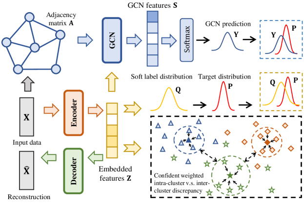
Figure 3: The network architecture of the proposed method DDAC-G. The original data $\mathbf{X}$ and adjacency matrix $\mathbf{A}$ serve as the input to the first GCN layer, and then the embedded features $\mathbf{S}$ and $\mathbf{A}$ serve as the input to each subsequent layer of GCN. The networks are jointly optimized via minimizing the data reconstruction loss, KL divergences between $\mathbf{Q}$ and $\mathbf{P}$ and between $\mathbf{Y}$ and $\mathbf{P}$, and the objective of confident weighted intra-cluster v.s. inter-cluster discrepancy.

Algorithm 2 Deep Discriminative Graph Clustering (DDAC-G)

Input: Data matrix $\mathbf{X}$, adjacency matrix $\mathbf{A}$, dimension of latent space $d^{\prime}$, number of clusters $k$, learning rate $\rho$, hyper-parameters $\beta$ and $\gamma$, threshold of confident assignment $\delta$, total training iterations $T_{iter}$.
Output: Cluster labels $C$.

1:  Initialize the network parameters $\Theta=\left\{\theta,\theta^{\prime}\right\}$ of AE with the pre-trained model;

2:  Initialize the cluster centroids $\bm{\mu}$ with $k$-means;

3:  for $iter=1$ to $T_{iter}$ do

4:     Obtain the learned latent representation $\mathbf{Z}$ of AE;

5:     Compute the soft label distribution $\mathbf{Q}$ by Eq. (6);

6:     Compute the target distribution $\mathbf{P}$ by Eq. (7);

7:     Compute the prediction $\mathbf{Y}$ of GCN by Eq. (16);

8:     Obtain the selective index set $\mathbf{t}$ by Eq. (8);

9:     Calculate $\mathcal{L}_{\textrm{recon}}$, $\mathcal{L}_{\textrm{clus}}$, $\mathcal{L}_{\textrm{disc}}$, and $\mathcal{L}_{\textrm{orth}}$ through Eq. (5), (12), (10), (11) respectively;

10:     Update the network parameters $\Theta$, $\left\{\bm{\mu}\right\}$, and $\mathcal{W}$ by minimizing Eq (13);

11:  end for

12:  Calculate the final cluster results as $c_{i}=\arg\max y_{ij}$.

13:  return  $C$.

Table 9: Network architecture of the extension of the proposed method (DDAC-G) for graph clustering.

Network	Encoder	Decoder
AE	Linear(784, 500), ReLU()	Linear(10, 2000),ReLU()
	Linear(500, 500), ReLU()	Linear(2000, 500),ReLU()
	Linear(500, 2000), ReLU()	Linear(500, 500),ReLU()
	Linear(2000, 10)	Linear(500, 784)
Network	GCN
GNN	GCN_Layer(784, 500), ReLU()
	GCN_Layer(500, 500), ReLU()
	GCN_Layer(500, 2000), ReLU()
	GCN_Layer(2000, 10) , ReLU()
	GCN_Layer(10, 10)

A.3 More experimental results

We further conduct experiment on a non-graph dataset HHAR and a graph dataset ACM, and the results are reported in Table 10. From this table, we see that the proposed DDAC-G method outperform most baseline methods with large margin. Besides, DDAC-G achieves 0.13%, 0.79%, 0.23% improvement in ACC, NMI and ARI on HHAR, and 0.15%, 0.23%, 0.32% improvement on ACM compared to state-of-the-art AGCN method. We also show the average scores of the three metrics in Figure 4 to provide an overall evaluation.

Table 10: Clustering performance on the non-graph dataset HHAR and the graph dataset ACM. Note that the results marked in bold denote the best clustering performance.

Methods/Data sets	HHAR (non-graph)			ACM (graph)
	ACC	NMI	ARI	ACC	NMI	ARI
$k$-means [MacQueen and others, 1967]	59.98$\pm$0.02	58.86$\pm$0.01	46.09$\pm$0.02	67.31$\pm$0.71	32.44$\pm$0.46	30.60$\pm$0.69
AE [Hinton and Salakhutdinov, 2006]	68.69$\pm$0.31	71.42$\pm$0.97	60.36$\pm$0.88	81.83$\pm$0.08	49.30$\pm$0.16	54.64$\pm$0.16
DEC [Xie et al., 2016]	69.39$\pm$0.25	72.91$\pm$0.39	61.25$\pm$0.51	84.33$\pm$0.76	54.54$\pm$1.51	60.64$\pm$1.87
IDEC [Guo et al., 2017]	71.05$\pm$0.36	74.19$\pm$0.39	62.83$\pm$0.45	85.12$\pm$0.52	56.61$\pm$1.16	62.16$\pm$1.50
GAE [Kipf and Welling, 2016]	62.33$\pm$1.01	55.06$\pm$1.39	42.63$\pm$1.63	84.52$\pm$1.44	55.38$\pm$1.92	59.46$\pm$3.10
VGAE [Kipf and Welling, 2016]	71.30$\pm$0.36	62.95$\pm$0.36	51.47$\pm$0.73	84.13$\pm$0.22	53.20$\pm$0.52	57.72$\pm$0.67
DAEGC [Wang et al., 2019]	76.51$\pm$2.19	69.10$\pm$2.28	60.38$\pm$2.15	86.94$\pm$2.83	56.18$\pm$4.15	59.35$\pm$3.89
ARGA [Pan et al., 2020]	63.30$\pm$0.80	57.10$\pm$1.40	44.70$\pm$1.00	86.10$\pm$1.20	55.70$\pm$1.40	62.90$\pm$2.10
SDCN [Bo et al., 2020]	84.26$\pm$0.17	79.90$\pm$0.09	72.84$\pm$0.09	90.45$\pm$0.18	68.31$\pm$0.25	73.91$\pm$0.40
AGCN [Peng et al., 2021]	88.11$\pm$0.43	82.44$\pm$0.62	77.07$\pm$0.66	90.59$\pm$0.15	68.38$\pm$0.45	74.20$\pm$0.38
DDAC-G	88.24$\pm$0.41	83.23$\pm$0.57	77.30$\pm$0.81	90.74$\pm$0.30	68.61$\pm$0.71	74.52$\pm$0.83

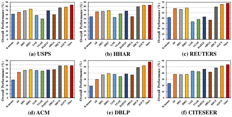
Figure 4: Comparison of each clustering method in terms of overall clustering performance. The proposed method achieves the best results on five datasets and is also comparable to the best performing DFCN on ACM.

To provide an intuitive comparison on clustering, we use t-SNE [Van Der Maaten and Hinton, 2008] to visualize the clustering performance on the USPS dataset. Figure 5 plots the visual comparison of raw data and the learned representations of SDCN and our method. We can observe that both SDCN and our method reveal better clustering structure compared to the original data distribution. Moreover, our method exhibits more compact intra-cluster structure, and more significant inter-cluster separation compared to SDCN, which implies that our method has learnt a more discriminative representation.

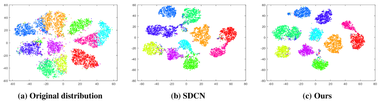
Figure 5: The t-SNE visualization of the learned representations from SDCN and our method on USPS dataset, and the original distribution serves as the baseline.

A.4 Parameter analysis

Analysis of hyper-parameters $\beta$ and $\gamma$.

We conduct the sensitivity analysis of two main hyper-parameters in our method, i.e., $\beta$ and $\gamma$ that control the contribution of the $\mathcal{L}_{\mathrm{disc}}$ and $\mathcal{L}_{\mathrm{orth}}$ in optimization. Specifically, we select USPS as the tested dataset, vary the values of $\beta$ and $\gamma$ from ${\left\{\textrm{1e-3},\cdots,\textrm{1e1}\right\}}$ and $\left\{\textrm{1e-6},\cdots,\textrm{1e0}\right\}$, and show the clustering performance in Figure 6. It can be seen that the our method has the best clustering performance when $\beta=\textrm{1e-3}$ and $\gamma=\textrm{1e-2}$, which indicates the effectiveness of these two terms. However, either excessive $\beta$ or $\gamma$ can negatively affect the clustering performance due to their overemphasis in the optimization. Therefore, we empirically give the recommended range of values for $\beta$ and $\gamma$ as from 1e-3 to 1e-1 and from 1e-5 to 1e-2, respectively.

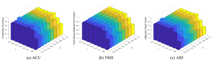
Figure 6: The sensitivity analysis of two hyper-parameters $\beta$ and $\gamma$ on USPS dataset. Note that the values of $\beta$ and $\gamma$ range from ${\left\{\textrm{1e-3},\cdots,\textrm{1e1}\right\}}$ and $\left\{\textrm{1e-6},\cdots,\textrm{1e0}\right\}$, respectively.

Analysis of the confident assignment threshold.

Figure 7 shows the clustering performance of our method under different confident assignment thresholds. We set the threshold to $\left\{0.1,\cdots,0.7\right\}$ for USPS, REUTERS, ACM, and DBLP, and $\left\{0.1,\cdots,0.6\right\}$ for HHAR and CITESEER since they fail to select eligible assignments when the threshold is set to 0.7. We can observe that filtering out some unconfident assignments by setting a threshold contributes to the clustering. Nevertheless, the clustering performance is negatively influenced if the threshold is set too high, because an excessively high threshold leads to select very few samples, which do not provide enough information of clusters. Furthermore, we can also find that the clustering performance of the ACM is only slightly affected by the threshold, which indicates that the graph of the ACM already provides good structural information available for the clustering task.

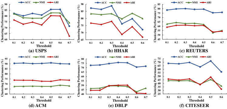
Figure 7: The performance comparison under different confident assignment thresholds, note that we set the threshold to $\left\{0.1,\cdots,0.6\right\}$ for HHAR and CITESEER since they fail to select eligible assignments when the threshold is set to 0.7.

Analysis of the number of nearest neighbors.

Since we use $k$NN to construct graphs for non-graph datasets, the clustering performance may be influenced by the value of $k$. Therefore, we set different number of nearest neighbors $k^{\prime}$ in $k$NN to evaluate the influence of their graphs constructed for non-graph data on the clustering performance. Specifically, we set $k^{\prime}$ to $\left\{1,3,5,10\right\}$ and present the clustering results in Figure 8. We can observe that the proposed DDAC-G method maintains stable clustering performance for different values of $k^{\prime}$, which demonstrates the robustness of the proposed method with regard to the variation of $k^{\prime}$. Nevertheless, it still achieves better performance at some specific $k^{\prime}$ values, such as setting $k^{\prime}$ to 3 for USPS and HHAR, and 1 for REUTERS.

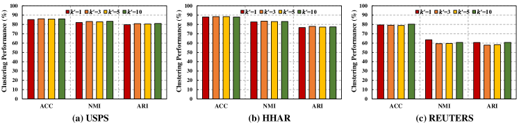
Figure 8: Clustering performance variation with different number of nearest neighbors $k^{\prime}$ in non-graph datasets. Note that $k^{\prime}$ is set to $\left\{1,3,5,10\right\}$, respectively.

References

- Abavisani et al. [2020] Mahdi Abavisani, Alireza Naghizadeh, Dimitris Metaxas, and Vishal Patel. Deep subspace clustering with data augmentation. Advances in Neural Information Processing Systems, 33:10360–10370, 2020.
- Bishop and Nasrabadi [2006] Christopher M Bishop and Nasser M Nasrabadi. Pattern recognition and machine learning, volume 4. Springer, 2006.
- Bo et al. [2020] Deyu Bo, Xiao Wang, Chuan Shi, Meiqi Zhu, Emiao Lu, and Peng Cui. Structural deep clustering network. In Proceedings of The Web Conference, pages 1400–1410, 2020.
- Chang et al. [2019] Jianlong Chang, Yiwen Guo, Lingfeng Wang, Gaofeng Meng, Shiming Xiang, and Chunhong Pan. Deep discriminative clustering analysis. arXiv preprint arXiv:1905.01681, 2019.
- Ding and Li [2007] Chris Ding and Tao Li. Adaptive dimension reduction using discriminant analysis and k-means clustering. In Proceedings of the International Conference on Machine Learning, pages 521–528, 2007.
- Elhamifar and Vidal [2013] Ehsan Elhamifar and René Vidal. Sparse subspace clustering: Algorithm, theory, and applications. IEEE transactions on pattern analysis and machine intelligence, 35(11):2765–2781, 2013.
- Fan [2021] Jicong Fan. Large-scale subspace clustering via k-factorization. In Proceedings of the ACM SIGKDD Conference on Knowledge Discovery & Data Mining, pages 342–352, 2021.
- Feng et al. [2020] Qiying Feng, Long Chen, CL Philip Chen, and Li Guo. Deep fuzzy clustering—a representation learning approach. IEEE Transactions on Fuzzy Systems, 28(7):1420–1433, 2020.
- Ghasedi Dizaji et al. [2017] Kamran Ghasedi Dizaji, Amirhossein Herandi, Cheng Deng, Weidong Cai, and Heng Huang. Deep clustering via joint convolutional autoencoder embedding and relative entropy minimization. In Proceedings of the IEEE International Conference on Computer Vision, pages 5736–5745, 2017.
- Guo et al. [2017] Xifeng Guo, Long Gao, Xinwang Liu, and Jianping Yin. Improved deep embedded clustering with local structure preservation. In Proceedings of the International Joint Conference on Artificial Intelligence, pages 1753–1759, 2017.
- Guo et al. [2019] Xifeng Guo, Xinwang Liu, En Zhu, Xinzhong Zhu, Miaomiao Li, Xin Xu, and Jianping Yin. Adaptive self-paced deep clustering with data augmentation. IEEE Transactions on Knowledge and Data Engineering, 32(9):1680–1693, 2019.
- Hartigan and Wong [1979] John A Hartigan and Manchek A Wong. Algorithm as 136: A k-means clustering algorithm. Journal of the Royal Statistical Society. Series C (Applied Statistics), 28(1):100–108, 1979.
- Hinton and Salakhutdinov [2006] Geoffrey E Hinton and Ruslan R Salakhutdinov. Reducing the dimensionality of data with neural networks. Science, 313(5786):504–507, 2006.
- Jain [2010] Anil K Jain. Data clustering: 50 years beyond k-means. Pattern recognition letters, 31(8):651–666, 2010.
- Ji et al. [2017] Pan Ji, Tong Zhang, Hongdong Li, Mathieu Salzmann, and Ian Reid. Deep subspace clustering networks. Advances in Nneural Information Processing Systems, 30:23–32, 2017.
- Jiang et al. [2017] Zhuxi Jiang, Yin Zheng, Huachun Tan, Bangsheng Tang, and Hanning Zhou. Variational deep embedding: an unsupervised and generative approach to clustering. In Proceedings of the International Joint Conference on Artificial Intelligence, pages 1965–1972, 2017.
- Kingma and Ba [2015] Diederik P Kingma and Jimmy Ba. Adam: A method for stochastic optimization. In Proceedings of the 3rd International Conference on Learning Representations, 2015.
- Kipf and Welling [2016] Thomas N Kipf and Max Welling. Variational graph auto-encoders. arXiv preprint arXiv:1611.07308, 2016.
- Kipf and Welling [2017] Thomas N. Kipf and Max Welling. Semi-supervised classification with graph convolutional networks. In Proceedings of the International Conference on Learning Representations, pages 1–14, 2017.
- Liu et al. [2013] G. Liu, Z. Lin, S. Yan, J. Sun, Y. Yu, and Y. Ma. Robust recovery of subspace structures by low-rank representation. IEEE Transactions on Pattern Analysis and Machine Intelligence, 35(1):171–184, 2013.
- Lv et al. [2021] Juncheng Lv, Zhao Kang, Xiao Lu, and Zenglin Xu. Pseudo-supervised deep subspace clustering. IEEE Transactions on Image Processing, 30:5252–5263, 2021.
- MacQueen and others [1967] James MacQueen et al. Some methods for classification and analysis of multivariate observations. In Proceedings of the Fifth Berkeley Symposium on Mathematical Statistics and Probability, volume 1, pages 281–297. Oakland, CA, USA, 1967.
- Matsushima and Brbic [2019] Shin Matsushima and Maria Brbic. Selective sampling-based scalable sparse subspace clustering. In Advances in Neural Information Processing Systems, pages 12416–12425, 2019.
- Mukherjee et al. [2019] Sudipto Mukherjee, Himanshu Asnani, Eugene Lin, and Sreeram Kannan. Clustergan: Latent space clustering in generative adversarial networks. In Proceedings of the AAAI Conference on Artificial Intelligence, volume 33, pages 4610–4617, 2019.
- Ng et al. [2001] Andrew Y Ng, Michael I Jordan, and Yair Weiss. On spectral clustering: Analysis and an algorithm. In Advances in Neural Information Processing Systems, volume 14, pages 849–856, 2001.
- Opochinsky et al. [2020] Yaniv Opochinsky, Shlomo E Chazan, Sharon Gannot, and Jacob Goldberger. K-autoencoders deep clustering. In Proceedings of the IEEE International Conference on Acoustics, Speech and Signal Processing, pages 4037–4041. IEEE, 2020.
- Pan et al. [2020] Shirui Pan, Ruiqi Hu, Sai-fu Fung, Guodong Long, Jing Jiang, and Chengqi Zhang. Learning graph embedding with adversarial training methods. IEEE Transactions on Cybernetics, 50(6):2475–2487, 2020.
- Peng et al. [2021] Zhihao Peng, Hui Liu, Yuheng Jia, and Junhui Hou. Attention-driven graph clustering network. In Proceedings of the ACM International Conference on Multimedia, pages 935–943, 2021.
- Peng et al. [2022] Xi Peng, Yunfan Li, Ivor W Tsang, Hongyuan Zhu, Jiancheng Lv, and Joey Tianyi Zhou. XAI beyond classification: Interpretable neural clustering. Journal of Machine Learning Research, 23(6):1–28, 2022.
- Shaol et al. [2018] Xuying Shaol, Keshi Ge, Huayou Su, Lei Luo, Baoyun Peng, and Dongsheng Li. Deep discriminative clustering network. In 2018 International Joint Conference on Neural Networks (IJCNN), pages 1–7, 2018.
- Shi and Malik [2000] Jianbo Shi and Jitendra Malik. Normalized cuts and image segmentation. IEEE Transactions on pattern analysis and machine intelligence, 22(8):888–905, 2000.
- Tang et al. [2020] Hui Tang, Ke Chen, and Kui Jia. Unsupervised domain adaptation via structurally regularized deep clustering. In Proceedings of the IEEE/CVF Conference on Computer Vision and Pattern Recognition, pages 8725–8735, 2020.
- Tu et al. [2021] Wenxuan Tu, Sihang Zhou, Xinwang Liu, Xifeng Guo, Zhiping Cai, En Zhu, and Jieren Cheng. Deep fusion clustering network. In Proceedings of the AAAI Conference on Artificial Intelligence, volume 35, pages 9978–9987, 2021.
- Tzoreff et al. [2018] Elad Tzoreff, Olga Kogan, and Yoni Choukroun. Deep discriminative latent space for clustering. arXiv preprint arXiv:1805.10795, 2018.
- Van Der Maaten and Hinton [2008] Laurens Van Der Maaten and Geoffrey Hinton. Visualizing data using t-sne. Journal of Machine Learning Research, 9:2579–2605, 2008.
- Veličković et al. [2018] Petar Veličković, Guillem Cucurull, Arantxa Casanova, Adriana Romero, Pietro Liò, and Yoshua Bengio. Graph attention networks. In Proceedings of the International Conference on Learning Representations, pages 1–12, 2018.
- Vidal [2011] René Vidal. Subspace clustering. IEEE Signal Processing Magazine, 28(2):52–68, 2011.
- Wang et al. [2019] C Wang, S Pan, R Hu, G Long, J Jiang, and C Zhang. Attributed graph clustering: A deep attentional embedding approach. In Proceedings of the International Joint Conference on Artificial Intelligence, 2019.
- Xie et al. [2016] Junyuan Xie, Ross Girshick, and Ali Farhadi. Unsupervised deep embedding for clustering analysis. In Proceedings of the International Conference on Machine Learning, pages 478–487. PMLR, 2016.
- Yang et al. [2016] Jianwei Yang, Devi Parikh, and Dhruv Batra. Joint unsupervised learning of deep representations and image clusters. In Proceedings of the IEEE/CVF Conference on Computer Vision and Pattern Recognition, pages 5147–5156, 2016.
- Yang et al. [2017] Bo Yang, Xiao Fu, Nicholas D Sidiropoulos, and Mingyi Hong. Towards k-means-friendly spaces: Simultaneous deep learning and clustering. In Proceedings of the International Conference on Machine Learning, pages 3861–3870. PMLR, 2017.
- Ye et al. [2007] Jieping Ye, Zheng Zhao, and Mingrui Wu. Discriminative k-means for clustering. Advances in Neural Information Processing Systems, 20, 2007.
- Zhang and Davidson [2021] Hongjing Zhang and Ian Davidson. Deep descriptive clustering. In Proceedings of the International Joint Conference on Artificial Intelligence, pages 3342–3348, 2021.
- Zhang et al. [2019] Tong Zhang, Pan Ji, Mehrtash Harandi, Wenbing Huang, and Hongdong Li. Neural collaborative subspace clustering. In Proceedings of the International Conference on Machine Learning, pages 7384–7393. PMLR, 2019.
- Zhang et al. [2020] Kaihua Zhang, Tengpeng Li, Shiwen Shen, Bo Liu, Jin Chen, and Qingshan Liu. Adaptive graph convolutional network with attention graph clustering for co-saliency detection. In Proceedings of the IEEE/CVF Conference on Computer Vision and Pattern Recognition, pages 9050–9059, 2020.
- Zhang et al. [2021] Shangzhi Zhang, Chong You, René Vidal, and Chun-Guang Li. Learning a self-expressive network for subspace clustering. In Proceedings of the IEEE/CVF Conference on Computer Vision and Pattern Recognition, pages 12393–12403, 2021.
- Zhao et al. [2021] Han Zhao, Xu Yang, Zhenru Wang, Erkun Yang, and Cheng Deng. Graph debiased contrastive learning with joint representation clustering. In Proceedings of the International Joint Conference on Artificial Intelligence, pages 3434–3440, 2021.