POODLE: Improving Few-shot Learning via Penalizing Out-of-Distribution Samples

Abstract

In this work, we propose to leverage out-of-distribution samples, i.e., unlabeled samples coming from outside target classes, for improving few-shot learning. Specifically, we exploit the easily available out-of-distribution samples (e.g., from base classes) to drive the classifier to avoid irrelevant features by maximizing the distance from prototypes to out-of-distribution samples while minimizing that to in-distribution samples (i.e., support, query data). Our approach is simple to implement, agnostic to feature extractors, lightweight without any additional cost for pre-training, and applicable to both inductive and transductive settings. Extensive experiments on various standard benchmarks demonstrate that the proposed method consistently improves the performance of pretrained networks with different architectures. Our code is available at https://github.com/lehduong/poodle.

1 Introduction

Learning with limited supervision is a key challenge to translate the research efforts of deep neural networks to real-world applications where large-scale annotated datasets are prohibitively costly to acquire. This issue has motivated the recent topic of few-shot learning (FSL), which aims to build a system that can quickly learn new tasks from a small number of labeled data.

A popular group of methods in FSL focus on strengthening the backbone network by various techniques, from increasing model capacity chen2019closer ; doersch2020crosstransformers , self-supervised learning (SSL) gidaris2019boosting ; su2020does ; zhang2021iept , to knowledge distillation (KD) tian2020rethinking . With these techniques, few-shot methods are expected to learn better representations that are more robust and generalized. However, even if the network can discover visual features and semantic cues, few-shot learners have to deal with a key challenge - the ambiguity: as we have only a small amount of support evidence, there are multiple plausible hypotheses at the inference stage. Existing works, therefore, rely on the developed inductive bias of the network (during the pretraining stage), such as shape bias ritter2017cognitive ; feinman2018learning , to reduce the hypothesis space.

In this work, we view the classification problem as conditional reasoning, i.e., “if X has P then X is Q”. Human beings are good at learning such inferences, thus quickly grasping new concepts with minimal supervision. More importantly, humans learn new concepts in context - where we have already had prior knowledge about other entities. According to mental models in cognitive science, when assessing the validity of an inference, one would retrieve counter-examples, i.e., which do not lead to the conclusion despite satisfying the premise de2005working ; edgington1995conditionals ; johnson2010mental ; verschueren2005everyday . Thus, if there exists at least one of such counter-examples, the inference is known to be erroneous.

Hence, we attempt to equip few-shot learning with the above ability so that it can eliminate incorrect hypotheses when learning novel tasks in a data-driven manner. Specifically, we leverage out-of-distribution data, i.e., samples belonging to classes separated from novel tasks , as counter-examples for preventing the learned prototypes from overfitting to their noisy features. To that end, when learning novel tasks, we adopt the large margin principle in metric learning weinberger2006distance to encourage the learned prototypes to be close to support data while being distant from out-of-distribution samples.

Our approach is complementary to existing works in FSL and could be combined to advance the state of the art. Moreover, our method is agnostic to the backbone network; thus, it does not have the need of a training phase to adopt as in SSL and KD, while incurring just a little overhead at inference (for fine-tuning prototypes with approximately 200 gradient updating steps).

In summary, our contributions are as follows:

• We propose a novel yet simple approach to learn the inductive bias of deep neural networks for FSL by leveraging out-of-distribution data. We empirically show that out-of-distribution data only require weak labels (i.e., in the form of whether a sample is in- or out-of-distribution) even in challenging problems such as cross-domain FSL.

• We introduce a new loss function to implement the above idea, which is applicable for both inductive and transductive inference. Our extensive experiments on different standard benchmarks show that the proposed approach consistently improves the performance of various network architectures.

• We validate the effectiveness of our method in various FSL settings, including cross-domain FSL.

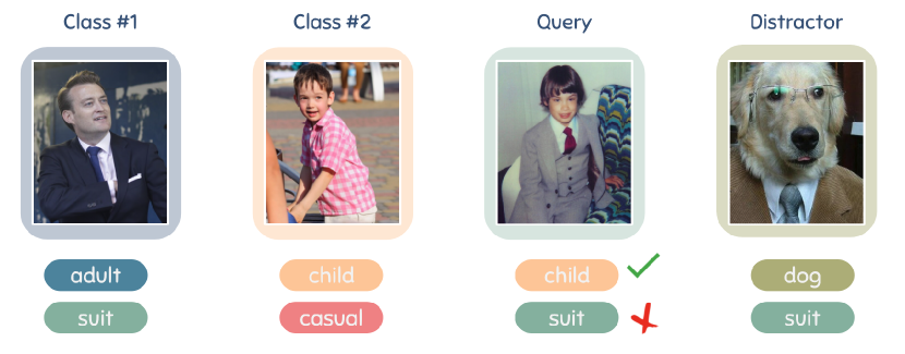
Figure 1: Illustration of advantages of counter-example data. The query image has features from both support classes (i.e., a child and a suit), which makes classification ambiguous. The prediction result would depend on the inductive bias or prior knowledge of the network. By using an out-of-distribution sample, it becomes clear that the query result should favor Class 2.

2 Related work

Over the past few years, considerable amount of research efforts finn2017model ; franceschi2018bilevel ; jamal2019task ; lee2018gradient ; qiao2018few ; matching_net ; prototypical_nets ; zhang2020deepemd have been invested in FSL. They can roughly be classified into two main categories: optimization-based and metric-based approaches. Optimization-based methods finn2017model ; franceschi2018bilevel ; jamal2019task ; lee2018gradient ; qiao2018few seek a meta-learner that can quickly adjust the parameters of another learner to a new task, given only a few support images. In particular, li2017meta ; finn2017model propose learning to initialize a classifier whose parameters can be obtained with a small number of gradient updates on the novel classes. Metric-based approaches matching_net ; prototypical_nets ; zhang2020deepemd learn a task-agnostic embedding space for measuring the similarity between images. For example, Matching Networks matching_net utilizes a weighted nearest neighbor classifier, while Prototypical Networks prototypical_nets uses the mean features of support images as the prototype for each class. Recently, DeepEMD zhang2020deepemd adopts the Earth Mover’s distance to compute the distance between image patches as their distance.

To further boost the performance, recent works have incorporated additional techniques such as self-supervised learning and knowledge distillation during training, and transductive inference during testing, which we will review in the following:

Self-supervised learning. The goal of self-supervised learning is to learn representations from unlabeled data. For FSL, this could be achieved by combining the supervised main task with a self-supervised pretext task which includes predicting image rotations gidaris2018unsupervised , predicting relative patch locations doersch2017multi , or solving jigsaw puzzles noroozi2016unsupervised . A few works incorporating self-supervised learning for FSL have been developed recently, e.g., Gidaris et al. gidaris2019boosting suggest pre-training the embedding network by using a combination of supervised and self-supervised loss, i.e., predicting image rotations.

Knowledge distillation. Knowledge distillation is a machine learning technique that seeks to compress the knowledge contained in a larger model (teacher) into a smaller one (student). It was introduced by Bucilua et al. bucilua2006model and later adopted to deep learning by Hinton et al. hinton2015distilling . Recently, Tian et al. tian2020rethinking show that incorporating self-distillation into FSL can boost the performance by $1-2\%$.

Transductive inference. Transductive inference aims to leverage the query set (which can be seen as unlabeled data during inference) in addition to the labeled support set. Transductive approaches liu2018learning ; hou2019cross ; qiao2019transductive ; ziko2020laplacian ; boudiaf2020transductive ; dhillon2019baseline significantly outperform their inductive counterparts, which do not exploit the query set. For example, TPN liu2018learning constructs a graph whose nodes are support and query images and propagates labels from the support to query images, while CAN hou2019cross utilizes confidently classified query images as part of the support set. Recently, TIM boudiaf2020transductive assumes a uniform distribution of novel classes, which is often the case for the current FSL benchmarks, and exploits that assumption for boosting the performance. Furthermore, finn2017model ; sung2018learning can be considered as transductive methods since the information from query data is used for batch normalization.

In this paper, we improve the performance of the classifier on novel classes by introducing a novel loss function, which penalizes out-of-distribution samples. Our method is complementary to the above approaches and can be combined to establish a new state-of-the-art for FSL. As the time of camera-ready, we are aware of a concurrent work das2021importance that also leverages the distractor samples to refine the classifier in FSL. Contrast to that work, our loss function is inherently applicable to both inductive and transductive inference. Furthermore, we also discover the effectiveness of uniform random features, which obviates the need for accessible OOD samples for in-domain FSL.

3 Preliminary

We first define some notations used in the following sections. Let $(\mathbf{x},y)$ consist of a sample image $\mathbf{x}$ and its corresponding class label $y$. Let $D_{b}=\{(\mathbf{x}_{i},y_{i})\}_{i=1}^{N_{b}}$ denote the labeled base samples used for feature pre-training. Next, we denote $D_{s}=\{(\mathbf{x}_{i},y_{i})\}_{i=1}^{N_{s}}$ and $D_{q}=\{(\mathbf{x}_{i},y_{i})\}_{i=1}^{N_{q}}$ as the labeled support samples and query samples respectively. Note that the labels for the query samples are only used for evaluation purposes. The support samples and query samples belong to the novel classes $C_{n}$, which are separated from the base classes $C_{b}$, i.e., $C_{b}\cap C_{n}=\varnothing$. In few-shot learning, we aim to learn a classifier that exploits support data to predict labels for query samples. We use a pre-trained feature extractor, usually kept fixed, to produce input to the classifier.

In this work, we consider fine-tuning the classifier on the support set only (inductive learning) and on both the support and query set (transductive learning). We also consider both in-domain and cross-domain FSL. In the former, the novel classes $C_{n}$ and the base classes $C_{b}$ are from the same domain (e.g., images from Image-Net), while for the latter, $C_{n}$ and $C_{b}$ are from different domains and the domains of $C_{b}$ and $C_{n}$ are referred to as the source and target domains, respectively.

Pretrained feature extractor.

Let $f_{\theta}$ be the feature extractor trained on the base data with the standard cross-entropy loss, which we also refer as the “simple baseline”. We also seek to strengthen the baseline with orthogonal techniques such as self-supervised learning (SSL) gidaris2019boosting ; su2020does and knowledge distillation (KD) tian2020rethinking . With SSL, we employ the “rot baseline”, which is trained with the standard cross-entropy loss and an auxiliary loss to predict the rotation angles of the perturbed images. We further apply the born-again strategy furlanello2018born for the rot baseline in two generations to construct the “rot + KD baseline”. More details of our baselines can be found in Section A.

Novel tasks inference.

In the few-shot scenario, we freeze the feature extractor $f_{\theta}$ and train a classifier for each task. Let $\mathbf{W}=[\mathbf{w}_{0},\cdots,\mathbf{w}_{k}]^{\top}\in\mathbb{R}^{K\times D}$ be the weight matrix of the classifier, where $D$ is the dimension of the encoded vector (output by the feature extractor) and $K$ is the number of classes (i.e., number of ways) for each task. The predictive distribution over classes $p(k|\mathbf{x}_{i},\mathbf{W})$ is given by:

$$p(k|\mathbf{x}_{i},\mathbf{W})=\frac{\exp(-\gamma\cdot d(\mathbf{z}_{i},\mathbf{w}_{k}))}{\sum_{j}\exp(-\gamma\cdot d(\mathbf{z}_{i},\mathbf{w}_{j}))},\quad\text{where}\quad\mathbf{z}_{i}=\frac{f_{\theta}(\mathbf{x}_{i})}{\|f_{\theta}(\mathbf{x}_{i})\|_{2}}$$ (1)

where $\gamma$ is the learnable scaling factor qi2018low and $d(\cdot,\cdot)$ denotes the distance function. We use the squared Euclidean distance in our experiments unless otherwise mentioned. In our implementation, we initialize each weight vector $\mathbf{w}_{k}$ to the mean of the sample features in the support set $\mathbf{w}_{k}=\frac{1}{|\mathcal{S}_{k}|}\sum_{\mathbf{x}\in\mathcal{S}_{k}}f_{\theta}(\mathbf{x})$ with $\mathcal{S}_{k}$ being the support set of the $k^{\mathrm{th}}$ class similar to Prototypical Network prototype .

Inductive bias.

Inductive learning is a process of learning a general principle by observing specific examples. Given limited support data, it is possible to have multiple explanations on the query data, with each corresponding to a different prediction. Inductive bias allows the learner to systematically favor one explanation over another, rather than favoring a model that overfits to the limited support data. Figure 1 shows an ambiguous classification example that can be explained by multiple hypotheses. Two decision rules possibly learnt from the support data are: 1) People in suit belong to class 1; and 2) Boys belong to class 2.

Both rules are simple (satisfying Occam’s razor), and can be used to classify the query sample. However, it is unclear which rule the learner would favor; it is only possible to know after training. Hence, solely learning with support data can be obscure. One way to narrow down the hypothesis space is using counter-examples to assess the inductive validity johnson2010mental ; de2005working . In Figure 1, the out-of-distribution (OOD) sample hints that the suit should be considered irrelevant, and hence the rule 1 should be rejected.

4 Proposed approach

We introduce our novel technique for few-shot learning namely Penalizing Out-Of-Distribution sampLEs (POODLE). Specifically, we attempt to regularize few-shot learning and improve the generalization of the learned prototypes by leveraging prior knowledge of in- and out-of-distribution samples. Our definition is as follows. Positive samples are in-distribution samples provided in the context of the current task that includes both support and query samples. Negative samples, in contrast, do not belong to the context of the current task, and hence are out-of-distribution. Negative samples can either provide additional cues that reduce ambiguity, or act as distractors to prevent the learner from overfitting. Note that negative samples should have the same domain as positive samples so that their cues are insightful to the learner, but positive and negative samples are not required to have the same domain as the base data.

To effectively use positive and negative samples in few-shot learning, the following conditions must be met: 1) The regularization guided by out-of-distribution samples can be combined with traditional loss functions for classification; 2) The regularization should be applicable for both inductive and transductive inference; and 3) The requirement on negative data should be minimal i.e., does not need any sort of labels except for aforementioned conditions.

4.1 Refining prototype with distractor samples

We formulate the regularization as a new objective function for training. To capitalize negative samples to reduce the ambiguity, we propose leveraging the large-margin principle as in Large Margin Nearest Neighbors (LMNN) weinberger2006distance ; weinberger2006distance . In these works, Weinberger et al. propose a loss function with two competing terms to learn a distance metric for nearest neighbor classification: a “pull” term to penalize the large distance between the embeddings of two nearby neighbors, which likely belong to the same class, and a “push” term to penalize the small distance between the embeddings of samples of difference classes.

In this work, we seek to learn prototypes for all categories instead of a distance metric. We do not have labels (i.e., categories) of all samples (e.g., transductive inference) but only the prior knowledge about whether a sample is in- or out-of-distribution. Thus, we adapt the above objective of margin maximization for these two groups, namely in- and out-of-distribution, with the distance function being the sum of distances from a sample to all prototypes. The goal is minimizing distances from positive samples to prototypes, while maximizing distances from negative samples to prototypes.

In our objective function, we keep the original “pull” term while introducing our new “push” term: we do not explicitly enforce large distances between positive samples and negative samples, but only attempt to maximize distances between prototypes and negative samples:

$$\mathcal{L}_{naive}=\sum_{i=1}^{N_{pos}}\sum_{k=1}^{K}\gamma\cdot d(\mathbf{w}_{k},\mathbf{x}_{i})-\sum_{j=1}^{N_{neg}}\sum_{k=1}^{K}\gamma\cdot d(\mathbf{w}_{k},\mathbf{x}_{j})$$ (2)

Note that $\gamma$ is scaling factor of distance-based classifier as in Equation 1. However, this objective does not take into account class assignments for positive samples. To tackle this problem, we use weighted distances between prototypes and samples to simultaneously optimize both objectives:

$$\mathcal{L}_{margin}=\underbrace{\sum_{i=1}^{N_{pos}}\sum_{k=1}^{K}\gamma\cdot d(\mathbf{w}_{k},\mathbf{x}_{i})\mathcal{S}_{G}[\,p(k|\mathbf{x}_{i},\mathbf{W})]}_{\mathcal{L}_{pull}}-\underbrace{\sum_{j=1}^{N_{neg}}\sum_{k=1}^{K}\gamma\cdot d(\mathbf{w}_{k},\mathbf{x}_{j})\mathcal{S}_{G}[\,p(k|\mathbf{x}_{j},\mathbf{W})]}_{\mathcal{L}_{push}}$$ (3)

where $\mathcal{S}_{G}[\cdot]$ is the stop-gradient operator. Intuitively, the positive sample will “pull” the prototypes to its location proportional to its distance to the prototypes. Subsequently, the prototype of each class will move closer to the positive samples of that class. At the same time, the prototype is enforced to move away from the negative samples, thus discarding features that might lead to high similarity to out-of-distribution data.

We note that removing $\mathcal{S}_{G}[\cdot]$ in Equation 3 would result in a different underlying objective, which empirically leads to a decrease in performance. Particularly, the objective without stop-gradient will also be compounded of an auxiliary term for entropy maximization (see Section B). Thus, devoid of meticulous regularization would deteriorate the performance. The above observation is in line with Boudiaf et al. boudiaf2020transductive . In summary, POODLE optimizes the classifier on novel tasks with the following objectives:

$$\boxed{\mathcal{L}_{\texttt{POODLE}}=\mathcal{L}_{ce}+\alpha\cdot\mathcal{L}_{pull}-\beta\cdot\mathcal{L}_{push}}$$ (4)

where $\alpha$ and $\beta$ control the “push” and “pull” coefficients respectively and $\mathcal{L}_{ce}$ denotes the standard cross-entropy loss. To the best of our knowledge, the proposed objective is the first loss function (in test phase) that can be effective for both inductive and transductive inference. Please see the supplemental document for the pseudo-code (Section C).

4.2 On negative samples

Choice of negative samples.

For in-domain FSL, we simply leverage the base data as negative samples. For cross-domain FSL, one approach would be using a set of samples drawn from classes that are disjoint to novel classes $C_{n}$ as negative examples. However, in some cases such negative examples might not be available. Thus, we consider another approach where we have a set of unlabeled data of a set of classes $C_{u}$ from the target domain ($C_{u}$ might overlap with $C_{n}$) as negative examples, similar to phoo2021selftraining . We name the above two approaches as disjoint and noisy negative sampling, respectively in the context of cross-domain FSL. Intuitively, when the number of categories of unlabeled data (i.e., $|C_{u}|$) grow larger, the noise of mixing positive and negative samples in noisy negative samples pool will be reduced.

The burden of additional data.

It is worth pointing out that POODLE does not break the setup of FSL as it does not require any additional data of novel classes, thus, still has a few samples from novel tasks. As POODLE obligates additional data in the form of OOD samples, one might ask how practical the algorithm is. For in-domain FSL, the negative samples can be easily obtained by adopting the training data as we already know $C_{n}\cap C_{b}=\varnothing$. Even in extreme case where we only have access to the pretrained models, we empirically find that ($\ell_{2}$-normalized) uniformly random noise can work surprisingly well (Section 4.3). For cross-domain FSL, even though POODLE requires additional OOD data, we find that these samples can be: 1) noisy with both positive and negative samples; and 2) fairly efficient - in our experiments, we can “reuse" $400$ OOD samples for all tasks, which is very efficient compared to other methods that might use up to $20\%$ unlabeled data of training set phoo2021selftraining .

4.3 Intriguing effectiveness of uniform random features

One caveat of POODLE is the obligation of accessing to OOD samples. Fortunately, we find that POODLE can use the uniform random features on the hypersphere as negative samples for in-domain FSL. Particularly, we can uniformly sample latent vectors from $\mathbb{S}^{D-1}$ as an alternative to the distractor samples from base training data, thus, eliminating the need for accessing to training data.

Our use of uniform distribution as negative examples is inspired by that feature uniformity is a desirable property for contrastive loss wang2020understanding ; chen2020intriguing , and so a good representation prefers such uniformity. The problem of uniformly distributing points on the unit hypersphere is related to minimizing pairwise loss kallenberg1997foundations ; borodachov2019discrete , which links well to the theory of supervised classification with softmax and cross-entropy (equivalent to minimizing pairwise loss or maximizing mutual information) boudiaf2020unifying ; qin2019rethinking .

Therefore, using uniform distribution as negative samples works for in-domain FSL because they will approximate the features of samples from base training data. For cross-domain FSL, this approach will fail because random features (which are similar to samples from the training domain) have a large discrepancy with the target domain, thus, not inducing meaningful cues. Intuitively, the more similar between domains of OOD and test samples, the higher performance gain POODLE can achieve. Our experiments in Section 5.4 empirically prove aforementioned postulation.

5 Experiments

In this section, we conduct extensive experiments to demonstrate the performance gain of our method on standard inductive, transductive, cross-domain FSL. To demonstrate the robustness of our method across datasets/network architectures, we keep the hyperparameters fixed for all experiments.

5.1 Experimental setup

Datasets.

We evaluate our approach on three common FSL datasets. The mini-Imagenet dataset matching_net consists of 100 classes chosen from the ImageNet dataset imagenet including 64 training, 16 validation, and 20 test classes with 60,000 images of size 84 $\times$ 84. The tiered-Imagenet tiered_imagenet is another FSL dataset which is also derived from the ImageNet dataset with 351 base, 97 validation, and 160 test classes with 779,165 images of size 84 $\times$ 84. Caltech-UCSD Birds (CUB) has 200 classes split into 100, 50, 50 classes for train, validation and test following chen2019closer . Furthermore, we also carry out experiments on iNaturalist 2017 (iNat) van2018inaturalist , EuroSAT helber2019eurosat , and ISIC-2018 (ISIC) codella2019skin for the (extreme) cross-domain FSL. The description for these datasets can be found in the supplemental document (Section D.1).

Implementation details.

We use ResNet12 as our feature extractor. It is a residual network ye2020few with 12 layers split into 4 residual blocks. For pre-training on the base classes, we train our backbones with the standard cross-entropy loss for 100 epochs. The optimizer has a weight decay of $5e^{-4}$, and the initial learning rate of 0.05 is decreased by a factor of 10 after 60, 80 epochs in mini-ImageNet and 60, 80, 90 epochs in tiered-ImageNet. We use the batch size of 64 for all the networks. For fine-tuning on the novel classes, we utilize Adam optimizer kingma2014adam with fixed learning rate of $0.001$, $\beta_{1}=0.9$, $\beta_{2}=0.999$, and do not use weight decay. The classifier is trained with 250 iterations. The coefficients of “push/pull” loss are $\alpha=1$ and $\beta=0.5$ respectively. For negative samples, we randomly select $K=400$ samples from the out-of-distribution samples pool for each novel task. We evaluate the performance of POODLE in 5-way-1-shot and 5-way-5-shot settings on 2000 random tasks with 15 queries each.

Table 1: Comparison to different baselines for the standard FSL (a.k.a in-domain FSL) on mini-ImageNet, tiered-Imagenet and CUB in the inductive setting with Resnet-12 as backbone. Here, POODLE-B and POODLE-R indicate that the negative samples are sampled from the base classes and the random uniform distribution respectively.

		mini-ImageNet		tiered-ImageNet		CUB
Baseline	Variant	1-shot	5-shot	1-shot	5-shot	1-shot	5-shot
Simple	CE Loss	61.33	80.76	67.42	84.44	75.60	89.88
	POODLE-B	63.79	81.41	69.26	84.97	75.96	90.06
	POODLE-R	64.38	81.35	69.34	85.03	76.22	89.99
Rot	CE Loss	64.57	82.89	68.26	85.09	76.39	91.10
	POODLE-B	66.78	83.65	69.74	85.45	77.26	91.30
	POODLE-R	67.20	83.54	69.86	85.56	77.35	91.43
Rot + KD	CE Loss	65.91	82.95	69.43	84.93	79.70	92.28
	POODLE-B	67.50	83.71	70.42	85.26	80.23	92.36
	POODLE-R	67.80	83.50	70.47	85.24	80.05	92.37

Table 2: Comparison to different baselines on mini-ImageNet, tiered-Imagenet and CUB with and without the proposed loss in the transductive settings. Here, $\mathcal{L}_{pull}^{b}$ and $\mathcal{L}_{pull}^{u}$ indicate that the negative samples are sampled from the base classes and the random uniform distribution respectively.

		mini-ImageNet		tiered-ImageNet		CUB
Baseline	Loss	1-shot	5-shot	1-shot	5-shot	1-shot	5-shot
Simple	$\mathrm{CE}$	61.33	80.76	67.42	84.44	75.60	89.88
	$\mathrm{CE}+\mathcal{L}_{pull}$	70.91	83.04	75.58	86.10	84.91	91.60
	$\mathrm{CE}+\mathcal{L}_{pull}-\mathcal{L}_{push}^{b}$	74.21	83.71	78.72	86.57	87.04	91.84
	$\mathrm{CE}+\mathcal{L}_{pull}-\mathcal{L}_{push}^{u}$	74.82	83.67	79.24	86.64	87.13	91.60
Rot	$\mathrm{CE}$	64.57	82.89	68.26	85.09	76.39	91.10
	$\mathrm{CE}+\mathcal{L}_{pull}$	74.42	85.20	76.59	86.75	85.93	93.02
	$\mathrm{CE}+\mathcal{L}_{pull}-\mathcal{L}_{push}^{b}$	77.30	85.91	79.74	87.25	88.68	93.23
	$\mathrm{CE}+\mathcal{L}_{pull}-\mathcal{L}_{push}^{u}$	77.69	85.86	80.31	87.33	89.07	93.35
Rot + KD	$\mathrm{CE}$	65.91	82.95	69.43	84.93	79.70	92.28
	$\mathrm{CE}+\mathcal{L}_{pull}$	74.90	85.09	77.07	86.50	88.22	93.68
	$\mathrm{CE}+\mathcal{L}_{pull}-\mathcal{L}_{push}^{b}$	77.56	85.81	79.67	86.96	89.88	93.80
	$\mathrm{CE}+\mathcal{L}_{pull}-\mathcal{L}_{push}^{u}$	77.24	85.53	79.97	86.91	90.02	93.68

5.2 Standard FSL

We first experiment with the standard FSL setup (also known as in-domain FSL) in which the number of query samples is uniformly distributed among classes.

Evaluation with various baselines. Table 1 shows the results of our approach with various baselines, which described in Section 3, with the inductive inference (positive samples are support images). As can be seen, our approach consistently boosts the performance of all baselines by a large margin (1-3$\%$). Interestingly, the POODLE-R variant outperforms the CE loss variant significantly and performs comparatively with the POODLE-B variant. We hypothesize that the normalized representations of the samples extracted from the base classes are uniformly distributed.

Table 2 demonstrates the efficacy of each loss term of POODLE in transductive inference (positive samples are support and query images). We can see that using the “pull” loss with query samples improve the inductive baseline significantly, being as effective as other transductive algorithms. Combining with “push” term, the classifier is further enhanced.

We also conduct experiments with additional loss functions including self-supervised loss (SSL) and knowledge distillation (KD) in Figure 2(a). Our approach consistently improves the generalization of all baselines without additional computation cost (in the training phase) as justified in Figure 2(b). The improvement of POODLE on other backbones and datasets is reported in the supplemental document (Section D.2).

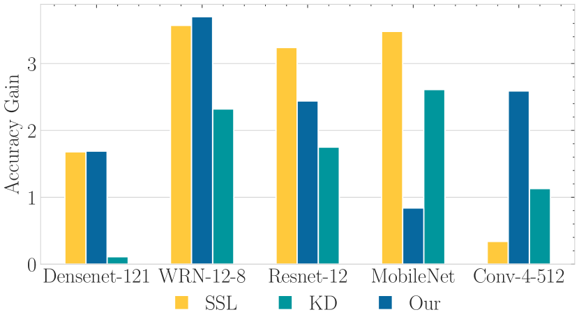
(a)

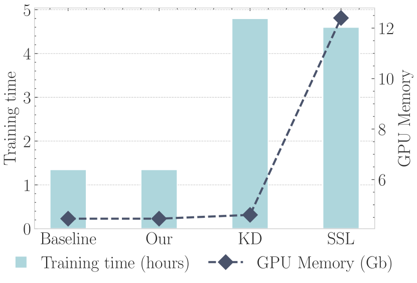
(b)

Figure 2: (a) Effectiveness of our approach applied to standard FSL. (a) Our approach consistently yields accuracy gains on different backbones, in comparison with those obtained by self-supervised loss (SSL) and knowledge distillation (KD) in 5-way-1-shot protocol on mini-Imagenet with inductive setting. (b) Total time and memory cost (in training stage) when adopting SSL, KD, and our method. Note that we apply KD for $T=2$ generation as in tian2020rethinking . No large overhead is incurred in our method.

Comparison to the state-of-the-art approaches.

We report the performance of our network in comparison with state-of-the-art methods in both transductive and inductive settings (with and without information from the query images) in Table 3. We can see that our approach remarkably improves the performance of the baseline and achieves a comparable performance with the state-of-the-art approaches in the tiered-ImageNet. In mini-ImageNet and CUB we significantly outperform the prior work in both inductive and transductive settings. Experimental results on other backbones are reported in the supplementary document (Section D.2).

Table 3: Comparison to the state-of-the-art methods on mini-ImageNet, tiered-Imagenet and CUB using inductive and transductive settings. The results obtained by our models (blue pearl-shaded) are averaged over 2,000 episodes.

			mini-ImageNet		tiered-ImageNet		CUB
Method	Transd.	Backbone	1-shot	5-shot	1-shot	5-shot	1-shot	5-shot
MAML finn2017model	✗	ResNet-18	49.6	65.7	-	-	68.4	83.5
RelatNet hou2019cross		ResNet-18	52.5	69.8	-	-	68.6	84.0
MatchNet matching_net		ResNet-18	52.9	68.9	-	-	73.5	84.5
ProtoNet prototypical_nets		ResNet-18	54.2	73.4	-	-	73.0	86.6
Neg-cosine liu2020negative		ResNet-18	62.3	80.9	-	-	72.7	89.4
MetaOpt lee2019meta		ResNet-12	62.6	78.6	66.0	81.6	-	-
SimpleShot simpleshot		ResNet-18	62.9	80.0	68.9	84.6	68.9	84.0
Distill tian2020rethinking		ResNet-12	64.8	82.1	71.5	86.0	-	-
Rot + KD + POODLE		ResNet-12	67.80	83.72	70.42	85.26	80.23	92.36
RelatNet + T hou2019cross	✓	ResNet-12	52.4	65.4	-	-	-	-
TPN liu2018learning		ResNet-12	59.5	75.7	-	-	-	-
TEAM qiao2019transductive		ResNet-18	60.1	75.9	-	-	-	-
Ent-min dhillon2019baseline		ResNet-12	62.4	74.5	68.4	83.4	-	-
CAN+T hou2019cross		ResNet-12	67.2	80.6	73.2	84.9	-	-
LaplacianShot ziko2020laplacian		ResNet-18	72.1	82.3	79.0	86.4	81.0	88.7
TIM-GD boudiaf2020transductive		ResNet-18	73.9	85.0	79.9	88.5	82.2	90.8
Simple + POODLE		ResNet-12	74.21	83.71	78.72	86.57	87.04	91.84
Rot + KD + POODLE		ResNet-12	77.56	85.81	79.67	86.96	89.93	93.78

5.3 Cross-domain FSL

In this section, we conduct experiments to demonstrate the efficacy of our approach even with a challenging task: extreme cross-domain FSL as first introduced in guo2020broader ; phoo2021selftraining . Many FSL algorithms are known to fail in such a challenging scenario chen2019closer .

Recall that we have two setups for cross-domain FSL (Section 4.2), in which cases, the negative samples are drawn from disjoint and noisy negative samples pool. Here, we provide the detailed setting of each scheme when transferring a network trained on mini-Imagenet to target domains. It is worth mentioning that we only consider inductive inference for comparison with prior work.

Disjoint negative samples. As mentioned before, we evaluate the results of cross-domain FSL on test split of these datasets while employing the train split to draw negative samples. Since the number of categories in EuroSAT and ISIC is relatively small (10 and 7 respectively) compare to the number of “way” in novel task (5), we only concern with iNat and CUB. Precisely, we follow chen2019closer and simpleshot to split CUB and iNat respectively.

Noisy negative samples. We assume that we have $20\%$ unlabeled data from the target domain and the rest $80\%$ of data is used for testing. Although a large number of classes are beneficial to POODLE as discussed above, we also carry out experiments with ISIC and EuroSAT to evaluate the performance of extreme cross-domain FSL with our approach.

From the Table 4 we can see that the improvement of POODLE with the disjoint negative samples (the bottom rows) and the noisy negative samples (the middle rows) when transferring knowledge from mini-ImageNet to iNat, CUB, ISIC, and EuroSAT. We can observe that despite the extreme gap between target/source domains and a very noisy mix of in- and out-of-distribution samples in negative samples pool (in case of EuroSAT and ISIC), POODLE can successfully boost the performance of baselines in all experiments. We also report the performance of other approaches, which have same setup as noisy negative samples, in Table 4.

Table 4: The results of the domain-shift setting from mini-Imagenet to CUB, iNat, ISIC, and EuroSAT with Rot + KD baseline. The results obtained by our models (blue pearl-shaded) are averaged over 2,000 episodes. The baselines with $\star$ notation show the results using the setup of disjoint negative samples, and the baselines without the $\star$ show the results using the setup of noisy negative samples.

	CUB		iNat		ISIC		EuroSAT
Baseline	1-shot	5-shot	1-shot	5-shot	1-shot	5-shot	1-shot	5-shot
Transfer phoo2021selftraining	-	-	-	-	30.71	43.08	60.73	80.30
SimCLR phoo2021selftraining	-	-	-	-	26.25	36.09	43.52	59.05
Transfer + SimCLR phoo2021selftraining	-	-	-	-	32.63	45.96	57.18	77.61
STARTUP (no SS) phoo2021selftraining	-	-	-	-	32.24	46.48	62.90	81.81
STARTUP phoo2021selftraining	-	-	-	-	32.66	47.22	63.88	82.29
Rot + KD + CE	49.98	69.44	48.90	66.58	32.35	43.81	65.00	80.01
Rot + KD + POODLE-R	50.04	69.78	48.94	66.87	32.21	43.87	63.97	79.85
Rot + KD + POODLE-B	52.61	70.78	50.62	67.31	33.56	44.17	66.21	80.51
Rot + KD + CE ⋆	50.28	69.64	48.80	66.72	-	-	-	-
Rot + KD + POODLE-R ⋆	50.25	69.97	48.84	67.03	-	-	-	-
Rot + KD + POODLE-B ⋆	53.11	70.96	50.46	67.45	-	-	-	-

5.4 Ablation study

In this section, we present results of some presentative ablation study to get more insight of POODLE behaviors. For more in-depth experiments, we refer reader to supplementary document.

5.4.1 The effect of domain discrepancy between positive-negative samples

Intuitively, the more similar between domains of OOD and test samples, the higher performance gain POODLE can achieve. To understand how our method works when OOD data is from various domains, we train our classifier and compare the performance when using random uniform distribution and other datasets as negative examples. The result of this experiment is reported in Table 5. We can observer that the more similar of OOD domain to test domain, the higher the performance gain we can achieve. Thus, we should always aim to leverage the OOD samples of test domain.

Table 5: Evaluating (simple) Resnet-12 trained on mini-Imagenet on different test/OOD domains in the 1-shot inductive protocol (10,000 episodes). random, mini, tiered, CUB, EuroSAT denote mini-Imagenet, tiered-Imagenet, CUB, EuroSAT dataset respectively. The OOD/test samples are drawn from the standard train/test split of each dataset, respectively. The 95% confidence interval is roughly 0.20 for all results.

		OOD domain
		w/o OOD	random	mini	tiered	CUB	EuroSAT
Test domain	mini	$61.63$	$\mathbf{64.30}$	$64.08$	$63.72$	$62.71$	$61.76$
	tiered	$63.04$	$64.28$	$64.01$	$\mathbf{64.50}$	$63.85$	$62.78$
	CUB	$48.55$	$48.88$	$49.01$	$49.10$	$\mathbf{51.40}$	$49.18$
	EuroSAT	$65.18$	$63.85$	$64.58$	$64.25$	$64.70$	$\mathbf{66.04}$

On the performance of random features:

For in-domain FSL i.e., test domains are mini-Imagenet and tiered-Imagenet, using uniform examples has the best and second-best accuracy when tested on mini-ImageNet and tiered-ImageNet, respectively. As aforesaid, the uniform random features will reflect the distribution of mini-Imagenet samples (which the network is pre-trained on). Thus, random features are effective for in-domain FSL.

For cross-domain FSL (i.e., test domains are CUB and EuroSAT), using random uniform features - which is approximately equal to using samples from mini-Imagenetet - does not work because the discrepancy between the source and target domain is extremely large, e.g., animal (mini-Imagenet) vs satellite images (EuroSAT).

5.4.2 Comparison against simple approaches for enhance pretrained models

Table 6: The results of the various approaches to learn a better classifier with pretrained Rot + KD baseline on mini-Imagenet. The results are obtained by averaging over 10,000 episodes.

Method	1-shot	5-shot
baseline	$66.32\pm 0.20$	$82.99\pm 0.13$
1) w/ learning cosine classifier	$66.66\pm 0.20$	$82.84\pm 0.13$
2) w/ naive OOD	$66.36\pm 0.20$	$83.08\pm 0.13$
3) w/ large-margin w/o negative samples	$66.32\pm 0.20$	$83.01\pm 0.13$
4) w/ label smoothing	$66.13\pm 0.20$	$80.81\pm 0.13$
POODLE-B	$\mathbf{67.84\pm 0.20}$	$\mathbf{83.72\pm 0.13}$
POODLE-R	$\mathbf{68.20\pm 0.20}$	$\mathbf{83.60\pm 0.13}$

To better understand the effectiveness of our method, we also compare to four methods that learn better classifiers on novel classes with pre-trained features. The results are reported in Table 6.

1. Learning cosine classifier: The classifier in inference phase is fine-tuned using CE loss with the support samples of each task. In our experiments, this approach does not bring any meaningful improvement similar to simpleshot .

2. Naive OOD: we fine-tune a $(k+1)$-way classifier with 1 additional class for OOD samples using CE loss. Naive OOD performs worse because the OOD samples are drawn from several classes of the training set, which are well-clustered and separated, we cannot find a "prototype" with a linear classifier to match all of them.

3. Large-margin w/o negative samples: only use push term in POODLE. This approach is not better than cosine-distance because the initialized prototype (mean of all samples from specific class) is already well-clustered and optimal i.e., close to the ground-truth class prototype and far away from others for the observed samples.

4. Label smoothing: we use label smoothing for CE loss (ground-truth class has the probability of 0.9 and uniformly distribute 0.1 to the rest. This method does not work well because it only makes learned prototypes not be far away from samples from other classes.

6 Conclusions and future work

In this work, we have proposed the concept of leveraging out-of-distribution samples set to improve the generalization of few-shot learners and realize it by a simple yet effective objective function. Our approach consistently boosts the performance of FSL across different backbone networks, inference types (inductive/transductive), and the challenging cross-domain FSL.

Future work might seek to exploit different sampling strategies (i.e., how to select negative samples) to further boost the performance and reduce time/memory complexity; another interesting direction is enhancing the robustness of the classifier when we have both positive and negative samples in the same sampling pool; leveraging domain adaptation to reduce the need of in-domain negative samples is also a promising research direction.

Appendix A Baseline Implementation

Simple Baseline.

As stated above, the simple baseline is constructed by training the feature extractor on base class with standard cross-entropy loss, which yield the objective function:

$${\color[rgb]{0,0,1}\mathcal{L}^{simple}}=\mathcal{L}_{clas}(\theta,\psi;D_{b})=\frac{1}{N_{b}}\sum_{i=0}^{N_{b}}\sum_{j=0}^{|C_{b}|}y_{ij}\log p_{\psi}(j|f_{\theta}(\mathbf{x}_{i}))$$ (5)

where $\theta$ and $\psi$ represent parameters of feature extractor and the linear classification, respectively.

Rotation Baseline.

For SSL, we implement the "rotation baseline” (Rot baseline). In detail, during global classification training, we rotate each image with all predefined angles: $\mathbf{x}_{i}^{r}=T(\mathbf{x}_{i},r)\forall r\in\mathcal{R}$ with $\mathcal{R}=\{0^{\circ},90^{\circ},180^{\circ},270^{\circ}\}$ and enforce the encoder to recognize the correct translation. Thus, the combined objective function of this baseline can be defined as:

$${\color[rgb]{1,0,0}\mathcal{L}^{rot}}={\color[rgb]{0,0,1}\mathcal{L}^{simple}}+\lambda_{ssl}\mathcal{L}_{ssl}(\theta,\phi;D_{b},\mathcal{R})$$ (6)

Precisely, we utilize a seperate classifier $g_{\phi}$ on top of feature extractor $f_{\theta}$ to predict the pertubation of images via cross-entropy loss with four classes corresponding to four possible translations similar to Gidaris et al. [18]. Accordingly, the SSL loss function $\mathcal{L}_{ssl}$ is given by:

$$\mathcal{L}_{ssl}(\theta,\phi;D_{b},\mathcal{R})=\frac{1}{N_{b}|\mathcal{R}|}\sum_{i=0}^{N_{b}}\sum_{j\in\mathcal{R}}\sum_{k=0}^{|\mathcal{R}|}\mathbb{I}(k=j)\log p_{\phi}(k|f_{\theta}(\mathbf{x}_{i}^{j}))$$ (7)

Here, $\mathbb{I}(\cdot)$ is the indicator function and $p_{\phi}(\cdot|f_{\theta})$ denotes the (predicted) probability of rotation angle.

Rotation + KD Baseline.

The "rotatiton + kd baseline” (Rot + KD baseline) is constructed by combining knowledge distillation [23] with rotation classification. Explicitly, we first train the feature extractor following the configuration of rotation baseline, and then exert the born-again strategy [17] to perform knowledge distillation for $T$ generations. The loss function of this baseline is given by:

$${\color[rgb]{1,.5,0}\mathcal{L}^{rot+kd}}={\color[rgb]{1,0,0}\mathcal{L}^{rot}}+\lambda_{kd\_clas}\mathcal{L}_{kd\_clas}(\theta_{t},\psi_{t};D_{b},\theta_{t-1},\psi_{t-1},\tau)+\\ \lambda_{kd\_ssl}\mathcal{L}_{kd\_ssl}(\theta_{t},\phi_{t};D_{b},\mathcal{R},\theta_{t-1},\phi_{t-1},\tau)$$ (8)

The above objectives optimize $\mathcal{L}_{clas}$ and $\mathcal{L}_{ssl}$ with both groundtruth labels along with the prediction from teacher models i.e., the model (of the same architecture) trained from the previous generation:

$$\mathcal{L}_{kd\_clas}(\theta_{t},\psi_{t};D_{b},\theta_{t-1},\psi_{t-1},\tau)=\frac{1}{N_{b}}\sum_{i=0}^{N_{b}}\sum_{j=0}^{|C_{b}|}p_{\psi_{t-1}}(j|f_{\theta_{t-1}}(\mathbf{x}_{i}),\tau)\log p_{\psi_{t}}(j|f_{\theta_{t}}(\mathbf{x}_{i}),\tau)$$ (9)

$$\mathcal{L}_{kd\_ssl}(\theta_{t},\phi_{t};D_{b},\mathcal{R},\theta_{t-1},\phi_{t-1},\tau)=\frac{1}{N_{b}|\mathcal{R}|}\sum_{i=0}^{N_{b}}\sum_{j\in\mathcal{R}}\sum_{k=0}^{|\mathcal{R}|}p_{\phi_{t-1}}(k|f_{\theta_{t-1}}(\mathbf{x}_{i}^{j}),\tau)\log p_{\phi_{t}}(k|f_{\theta_{t}}(\mathbf{x}_{i}^{j}),\tau)$$ (10)

Following Tian et al. [52], we distill the network for $T=2$ generations and use the last checkpoint of previous generation as the teacher for next generation. For simplicity, we set the hyperparameters $\lambda_{ssl}=\lambda_{kd\_ssl}=\lambda_{kd\_clas}=1$ and $\tau=4$ for all experiments.

Appendix B On the importance of stop-gradient operator

In this section, we elaborate the bleak outcome when removing the stop-gradient operator of loss function in Equation 3. As discussed before, the soft-weight in “pull/push” loss terms should be used to guide the degree of force. Directly optimize these soft weights would lead to different underlying objective that jointly maximizing conditional entropy as we show below.

First, we define the objective function (for each positive/negative term) in Equation 3 as weighted distance loss:

$$\mathcal{L}_{wd}=\sum_{k=1}^{K}\gamma\cdot d(\mathbf{w}_{k},\mathbf{x}_{i})\mathcal{S}_{G}[\,p(k|\mathbf{x}_{i},\mathbf{W})]$$ (11)

Furthermore we define the log-sum-exp loss function as:

$$\mathcal{L}_{lse}=-\log\sum_{k=1}^{K}\exp(-\gamma\cdot d(\mathbf{w}_{k},\mathbf{x}_{i}))$$ (12)

Lemma B.1.

The two loss function $\mathcal{L}_{wd}$ and $\mathcal{L}_{lse}$ have same set of solutions.

Proof. This can be proved by taking the gradient of two terms w.r.t. $j^{\text{th}}$ prototype. Particularly, the gradient of $\mathcal{L}_{lse}$ w.r.t. $\mathbf{w}_{j}$ is given by:

$$\frac{\partial\mathcal{L}_{lse}}{\partial\mathbf{w}_{j}} =-\frac{\partial\log\sum_{k=1}^{K}\exp(-\gamma\cdot d(\mathbf{w}_{k},\mathbf{x}_{i}))}{\partial\mathbf{w}_{j}}$$ (13)

$$=-\frac{1}{\sum_{k=1}^{K}\exp(-\gamma\cdot d(\mathbf{w}_{k},\mathbf{x}_{i}))}\times\frac{\partial\sum_{k=1}^{K}\exp(-\gamma\cdot d(\mathbf{w}_{k},\mathbf{x}_{i}))}{\partial\mathbf{w}_{j}}$$ (14)

$$=-\frac{\exp(-\gamma\cdot d(\mathbf{w}_{j},\mathbf{x}_{i}))}{\sum_{k=1}^{K}\exp(-\gamma\cdot d(\mathbf{w}_{k},\mathbf{x}_{i}))}\times\frac{\partial(-\gamma\cdot d(\mathbf{w}_{j},\mathbf{x}_{i}))}{\partial\mathbf{w}_{j}}$$ (15)

$$=p(j|\mathbf{x}_{i},\mathbf{W})\cdot\frac{\partial\big{(}\gamma\cdot d(\mathbf{w}_{j},\mathbf{x}_{i})\big{)}}{\partial\mathbf{w}_{j}}$$ (16)

On the other hand, the gradient of $\mathcal{L}_{wd}$ term w.r.t. to $\mathbf{w}_{j}$ is given by:

$$\frac{\partial\mathcal{L}_{wd}}{\partial\mathbf{w}_{j}} =\frac{\partial\sum_{k=1}^{K}\gamma\cdot d(\mathbf{w}_{k},\mathbf{x}_{i})\mathcal{S}_{G}[\,p(k|\mathbf{x}_{i},\mathbf{W})]}{\partial\mathbf{w}_{j}}$$ (17)

$$=p(j|\mathbf{x}_{i},\mathbf{W})\frac{\partial\big{(}\gamma\cdot d(\mathbf{w}_{j},\mathbf{x}_{i})\big{)}}{\partial\mathbf{w}_{j}}$$ (18)

Thus, both loss function should optimize the same underlying objective.

Corollary B.1.1.

Taking out the stop-gradient operator in “weighted distance” loss results in a objective that jointly minimizing conditional entropy of label given raw features and weighted distance (i.e., the old loss function).

Proof: We refer to this objective function as “Expected Distance” loss. We can prove above corollary by rewriting the objective function as below:

$$\mathcal{L}_{ed} =\sum_{k=1}^{K}\gamma\cdot d(\mathbf{w}_{k},\mathbf{x}_{i})\,p(k|\mathbf{x}_{i},\mathbf{W})=-\sum_{k=1}^{K}p(k|\mathbf{x}_{i},\mathbf{W})\log\Big{[}\exp\big{(}-\gamma\cdot d(\mathbf{w}_{k},\mathbf{x}_{i})\big{)}\Big{]}$$ (19)

$$=-\sum_{k=1}^{K}\Big{[}p(k|\mathbf{x}_{i},\mathbf{W})\log\frac{\exp(-\gamma\cdot d(\mathbf{w}_{k},\mathbf{x}_{i}))}{\sum_{k^{\prime}}\exp(-\gamma\cdot d(\mathbf{w}_{k^{\prime}},\mathbf{x}_{i}))}+p(k|\mathbf{x}_{i},\mathbf{W})\log\sum_{k^{\prime}}\exp(-\gamma\cdot d(\mathbf{w}_{k^{\prime}},\mathbf{x}_{i}))\Big{]}$$ (20)

$$=\underbrace{\Big{(}-\sum_{k=1}^{K}p(k|\mathbf{x}_{i},\mathbf{W})\log p(k|\mathbf{x}_{i},\mathbf{W})\Big{)}}_{\text{conditional entropy loss}}-\underbrace{\log\sum_{k^{\prime}}\exp\big{(}-\gamma\cdot d(\mathbf{w}_{k^{\prime}},\mathbf{x}_{i})\big{)}}_{\text{``old'' loss}}$$ (21)

Using the Lemma B.1 and Equation 21, we can observe that without the stop-gradient operator, underlying objective combining empirical (Monte-Carlo) estimate of conditional entropy of label given extracted features and “weighted” distance (i.e., “old” loss).

Discussion.

As noted by Boudiaf et al. [2], optimizing the conditional entropy loss requires special scrutiny, since the optima could result in trivial solutions on the simplex vertices i.e., assigning all samples to a single class. Particularly, a small value of learning rate and fine-tuning the whole network (similar to [10]) are crucial to prevent dramatical deterioration in performance. In their experiments [2], they found that training the classifier with conditional entropy and cross-entropy loss signficant decrease the performance of few-shot learner. Beside, utilizing the conditional entropy for “push” loss does not affect the performance of classifier since it does not lead to collapsed solutions.

Appendix C Pseudo Code

We provide the pseudo-code of POODLE in a coding style similar to Pytorch as in Algorithm 1.

⬇

# f: classifier

# support: support images

# support_labels: labels of support images

# query: query images

# alpha: weight of positive term

# beta: weight of negative term

# sample negative data

neg_data = sample_from_train_set()

# construct positive data

if transductive:

n_support = support.size(0)

pos_data = concatenate([support, query])

else:

pos_data = support

for i in range(n_steps):

# compute logits

pos_out = f(pos_data)

neg_out = f(neg_data)

# compute POODLE loss

pull_loss = sum(pos_out * softmax(pos_out).detach())

push_loss = sum(neg_out * softmax(neg_out).detach())

poodle_loss = alpha * pull_loss - beta * push_loss

# compute CE loss

ce_loss = sum(support_label * log_softmax(pos_out[: n_support]))

loss = ce_loss + poodle_loss

# optimization step

loss.backward()

optimizer.step()

Algorithm 1 PyTorch-style pseudocode for POODLE.

Appendix D Additional results

In this section, we provide more experimental results when applying POODLE for various network architectures and conducting ablation study to verify its effectiveness under numerous configurations. Note that by POODLE, we refer to POODLE-B i.e., negative samples are drawn from base classes, unless otherwise state.

D.1 Dataset

In this section, we briefly describe the datasets used for evaluating performance of cross-domain FSL below.

• iNatural-2017 [59]: This heavy-tailed dataset consists of $859,000$ images from over $5,000$ species of plants and animals. For disjoint negative sampling, we follow the meta-iNat benchmark [59, 57] i.e., splitting the dataset to $908$ classes for sampling negative samples and $227$ classes for evaluation.

• EuroSAT [22]: This dataset covers total $27,000$ labeled images of Sentinel-2 satellite images, which consist of $10$ classes and the patches measure $64\times 64$ pixels.

• ISIC-2018 (ISIC) [7]: This dataset covers dermoscopic images of skin lesions. Precisely, we use the training set for task $3$ (i.e., lesion disease classification), which contains $10,015$ images with $7$ ground truth classification labels.

It is worth mentioning that, for the sake of simplicity, we apply the same image transformation as in mini-Imagenet to these cross-domain datasets. Thus, the resolution of processed images of cross-domain datasets are $84\times 84$ in our implementation. In contrast, the benchmark protocol using the image resolution of $224\times 224$ [21]. A higher image resolution helps improve the performance of classifier significantly as we demonstrate in Section D.5.4. Nevertheless, POODLE successfully boosts the performance of all baselines in cross-domain FSL by a large margin.

D.2 Standard FSL

In this section, we provide the experimental results of backbones other than Resnet-12. Specifically, we consider widely adopted architectures, namely Conv-4-512 [55], WideResnet [62], Mobilenet [25], and Densenet [27]. Particularly:

• Conv-4-512: We follow [55] to implement this architecture. More concretely, it is consisted of $4$ convolutional layers with hidden channels of $64$ and the output dimension is $512$.

• WRN-28-10 [62]: We follow [48, 57] and use the wide residual network with $28$ convolutional layers and widening factor of $10$.

• DenseNet-121 [27]: Similar to [57], we adopt the $121$-layers architecture while removing the first two-down sampling layers and using the kernel size of $3\times 3$ for the first convolutional layer.

• MobileNet [25]: We follow [57] and use the standard MobileNet for ImageNet [25] but remove the first two down-sampling layers of the network.

For all aforementioned architectures, we adopt the same training configuration of Resnet-12 as described in Section 5, excepts for WRN-28-10 we use the batch size of $32$ for all datasets. Beside that, we use the negative samples from base classes i.e., POODLE-B in all experiments unless otherwise stated.

Table 7 shows the improvement of POODLE with various backbones of different network architectures on mini-Imagenet. We can see that our approach consistently enhance the accuracy of all baselines by a large margin i.e., $2-4\%$ in $1$-shot protocol and $0.5-1\%$ in $5$-shot protocol.

In Table 8, we present the comparison between performance achieved by WRN-28-10 with our approach and other algorithms on mini- and tiered-Imagenet. It can be observed that combining POODLE with other techniques such as SSL and KD achieves comparable or outperform state-of-the-art techniques for both inductive/transductive inference on two datasets.

Table 7: Comparison to different baselines for the standard FSL (a.k.a in-domain FSL) on mini-ImageNet with various network architectures. The results are evaluated with $10,000$ random sampled tasks. The $95\%$ confidence interval of $1$-shot and $5$-shot classification are roughly $0.2$ and $0.1$, respectively.

			Inductive		Transductive
Network	Baseline	Variant	1-shot	5-shot	1-shot	5-shot
WRN-28-10	Simple	CE Loss	61.23	81.08	61.23	81.08
		POODLE	64.94	81.88	71.49	83.48
	Rot	CE Loss	64.77	83.66	64.77	83.66
		POODLE	68.27	84.45	75.24	85.95
	Rot + KD	CE Loss	67.12	84.15	67.12	84.15
		POODLE	69.67	84.84	77.30	86.34
DenseNet-121	Simple	CE Loss	64.88	81.99	64.88	81.99
		POODLE	66.53	82.55	75.55	84.62
	Rot	CE Loss	66.51	83.92	66.51	83.92
		POODLE	68.68	84.52	77.85	86.49
	Rot + KD	CE Loss	68.66	84.17	68.66	84.17
		POODLE	70.29	84.80	78.57	84.49
Conv-4-512	Simple	CE Loss	50.90	70.44	50.90	70.44
		POODLE	53.60	71.08	58.61	72.78
	Rot	CE Loss	51.36	70.81	51.36	70.81
		POODLE	54.04	71.69	58.84	73.24
	Rot + KD	CE Loss	51.46	70.42	51.46	70.42
		POODLE	53.87	71.36	58.50	72.87
MobileNet	Simple	CE Loss	60.99	77.45	60.99	77.45
		POODLE	61.75	77.87	70.63	80.04
	Rot	CE Loss	64.57	80.86	64.57	80.86
		POODLE	65.45	81.37	74.81	83.50
	Rot + KD	CE Loss	65.41	80.60	65.41	80.60
		POODLE-I	66.02	81.18	74.55	83.09

Table 8: Comparison to the state-of-the-art methods on mini-ImageNet, and tiered-Imagenet using inductive and transductive settings on WRN-28-10. The results obtained by our models (pear-shaded) are averaged over $10,000$ episodes.

		mini-ImageNet		tiered-ImageNet
Method	Transd.	1-shot	5-shot	1-shot	5-shot
LEO [48]	✗	61.8	77.6	66.3	81.4
SimpleShot [57]		63.5	80.3	69.8	85.3
MatchNet [55]		64.0	76.3	-	-
CC+rot+unlabeled [18]		64.0	80.7	70.5	85.0
FEAT [61]		65.1	81.1	70.4	84.4
Simple		61.23	81.08	67.63	83.93
Simple + POODLE		64.94	81.88	70.25	84.64
Rot + KD		67.12	84.15	-	-
Rot + KD + POODLE		69.67	84.84	-	-
AWGIM [20]	✓	63.1	78.4	67.7	82.8
Ent-min [10]		65.7	78.4	73.3	85.5
SIB [26]		70.0	79.2	-	-
BD-CSPN [37]		70.3	81.9	78.7	86.92
LaplacianShot [65]		74.9	84.1	80.2	87.6
TIM-ADM [2]		77.5	87.2	82.0	89.7
TIM-GD [2]		77.8	87.4	82.1	89.8
Simple + POODLE		71.49	83.48	76.27	85.83
Rot + KD + POODLE		77.30	86.34	-	-

D.3 Results of reimplemented transductive algorithms

In this section, we report the accuracy of our reimplemented of transductive algorithms and their originally reported performance (balanced query set). In Table 9, we present the performance of our reproduced transductive algorithms (on Resnet-12). We can see that our implementation achieve comparable or higher accuracy than the original work even though we adopt the more efficient architecture (i.e., Resnet-12 compared to Densenet).

Table 9: Results of our implementations of various transductive methods compared to original works on mini-ImageNet. The results of our implementations (pear-shaded) are evaluated on Resnet-12 + Rot + KD baseline with 2,000 random sampled tasks.

Methods	Network	1-shot	5-shot
Mean-shift	Resnet-12	$73.49\pm 0.55$	$84.24\pm 0.32$
Mean-shift [35]	DenseNet-121	$71.39\pm 0.27$	$82.67\pm 0.15$
Bayes k-means	Resnet-12	$71.40\pm 0.50$	$83.79\pm 0.31$
Bayes k-means [35]	DenseNet-121	$72.05\pm 0.24$	$80.34\pm 0.17$
Soft k-means	Resnet-12	$74.55\pm 0.49$	$84.53\pm 0.30$
Soft k-means [45]	Conv-4-64	$50.09\pm 0.45$	$64.59\pm 0.28$
CAN_T	Resnet-12	$71.04\pm 0.53$	$84.21\pm 0.30$
CAN_T [24]	Resnet-12	$67.19\pm 0.55$	$80.64\pm 0.35$
TIM	Resnet-12	$77.69\pm 0.55$	$87.40\pm 0.29$
TIM [2]	Resnet-18	$73.90\pm n/a$	$85.00\pm n/a$

D.4 Imbalanced query set

So far, prior works in (transductive) FSL mainly concern with balanced query samples i.e., numbers of query images for each class are equal. However, in practice, there is no guarantee that this setting is hold. In this section, we conduct experiments to benchmark the performance of different transductive algorithms under class-skew i.e., imbalanced query data. We simulate the long-tail distribution of the query samples through the Dirichlet distribution. Precisely, for each novel task, we sample the number of queries for every category from a Dirichlet distribution with concentration $\kappa$ for all classes so that the total number of query images is always $75$ (similar to the experiments in the previous section).

In the “pull” loss term, we employ a “soft” weights for minimizing distance between prototypes and samples without any explicit regularization for distance between prototypes. In conventional setup for transductive learning, the number of query samples of each category are uniformly distributed, hence, the positive samples of each category implicitly constrains the prototype by “pulling” corresponding prototype. Under an extremely imbalanced query set, the positive samples from the dominated class might pull all the prototypes to their region by learning similar features of samples from different classes. In that case, increasing the value of $\beta$ to prevent the collapsed solution is necessary.

Table 10 presents the results of different transductive learning algorithms under the imbalanced query set. The detailed performance of the reproduced algorithms compared to the original papers are reported in Section D.3. The coefficient of “push” term is set to $\alpha=1$. Since TIM [2] explicitly use the uniform distribution information of samples in the query set, its performance drastically drops in the imbalanced FSL. Other variants of K-means are more robust to the long-tail distribution, but they are far inferior to POODLE with $\beta=0.75$.

Table 10: Results of transductive learning on imbalance query data of mini-ImageNet. The results obtained by our models (blue pearl-shaded) are averaged over 2,000 episodes. $\kappa$ denotes the concentration parameter of the Dirichlet distribution.

	$\kappa=0.5$		$\kappa=1$		$\kappa=2$		$\kappa=5$
Methods	1-shot	5-shot	1-shot	5-shot	1-shot	5-shot.	1-shot	5-shot
Inductive	66.91	82.75	66.16	82.62	66.10	83.01	66.23	83.16
Mean-shift [35]	68.88	80.54	70.31	81.82	71.78	83.16	72.92	83.98
Bayes k-means [35]	69.69	82.86	69.91	82.95	70.64	83.54	71.39	83.83
Soft k-means [45]	65.31	75.65	68.61	78.90	71.56	81.58	73.45	83.33
CAN_T [24]	72.30	83.53	71.28	83.62	71.09	84.06	71.18	84.25
TIM [2]	47.65	52.79	54.86	61.32	61.84	68.73	68.74	76.39
POODLE-B $\beta=0.00$	61.16	76.40	66.02	79.88	70.03	82.43	73.03	84.23
POODLE-B $\beta=0.50$	64.56	81.01	69.14	83.63	72.91	85.14	75.79	85.78
POODLE-B $\beta=0.75$	75.20	86.51	74.06	86.17	74.77	86.48	74.74	86.34
POODLE-B $\beta=1.00$	75.48	88.36	71.14	86.31	70.20	85.53	68.94	84.31

D.5 Ablation study

D.5.1 Removing stop-gradient operator

As discussed before in Section B, the stop-gradient operator is of paramount important to avoid trivial solutions. In this section, we consider different choice of usage of the stop-gradient operator namely not using it in both “push/pull” terms, use only with one of two term, and use it for both terms in Table 11.

From the table, we can see that the stop-gradient operator does not affect the performance much in inductive inference. It can be explained as the posterior distribution of support data already has a high probability for “correct” classes and the conditional entropy term does not affect much. In transductive inference, removing the stop-gradient operator on “pull” term results in noticeable decrease in accuracy as we articulate in Section B. On the other hand, taking out stop-gradient operator on “push” term does not worsen the performance since it does not lead to trivial solutions.

Table 11: Results of different settings of stop-gradient in push and pull terms. The results are evaluated with $2,000$ random sampled tasks on Resnet-12 with Rot + KD baseline. The $95\%$ confidence interval of $1$-shot and $5$-shot classification are roughly $0.45$ and $0.3$ for inductive setting and $0.6$ and $0.4$ for transductive, respectively. Results of inductive baseline for $1$-shot and $5$-shot are $65.91\pm 0.44$ and $82.95\pm 0.30$, respectively.

	Stop-grad		Inductive		Transductive
Method	Pull	Push	1-shot	5-shot	1-shot	5-shot
POODLE-B	✓	✓	67.52	83.71	77.58	85.87
	✗	✓	67.50	83.56	62.04	82.87
	✓	✗	67.37	83.73	78.51	86.28
	✗	✗	67.37	83.64	72.04	85.08
POODLE-R	✓	✓	67.80	83.50	77.25	85.52
	✗	✓	67.80	83.39	66.55	83.65
	✓	✗	67.77	83.43	78.11	85.83
	✗	✗	67.77	83.36	73.29	84.77

D.5.2 Sensitive to $\alpha$ and $\beta$

So far, we only fixed the coefficient of “push/pull” loss with $\alpha=1$ and $\beta=0.5$, we now consider different configurations of these parameters to understand the sensitive of POODLE to these hyper-parameters. Precisely, we report the accuracy gain of POODLE with different combination of $\alpha$ and $\beta$ taken from the list $[0.0,0.25,0.5,0.75,1.0,2.0,5.0]$ as in Figure 3.

We can observe from Figure 3 that POODLE is robust to the change of $\alpha$ and $\beta$: the accuracy of network is improved as long as the value of $\alpha$ is larger than $\beta$. Furthermore, the improvement in accuracy usually does not change much when varying $\alpha$ and $\beta$.

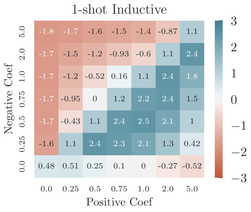
(a) 1-shot Inductive Inference

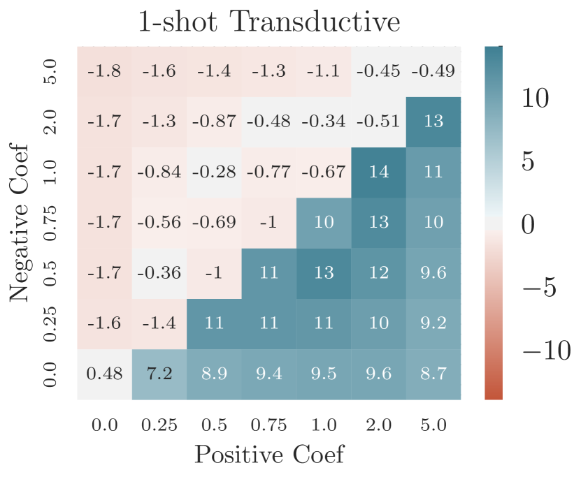
(b) 1-shot Transductive Inference

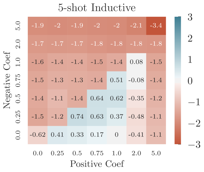
(c) 5-shot Inductive Inference

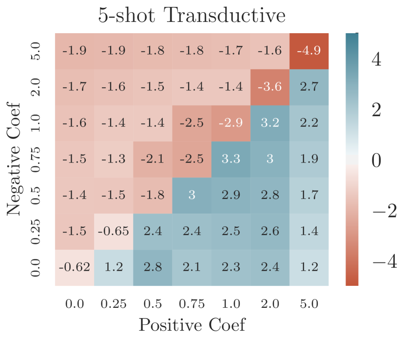
(d) 5-shot Transductive Inference

Figure 3: Ablation study on the affect of positive and negative coefficient of POODLE (i.e., $\alpha$ and $\beta$) to accuracy gain of (simple baseline) Resnet-12 on mini-Imagenet compared to no fine-tuning at all with $10,000$ random tasks. The baseline where we directly assign the prototype of each class to the mean of its support images obtains accuracy of $61.63\pm 0.20$ and $80.78\pm 0.11$ for $1$-shot and $5$-shot classification, respectively.

D.5.3 Number of sampled negative data

Intuitively, a larger number of negative samples will provide more informative cues to the classifer, however, they might require a notable memory footprint and have significant latency. We conduct experiment to quantify the impact of number of negative samples to the accuracy of POODLE in Table 12. These results indicate that higher number of negative samples consistently leads to better performance, however, the gain in accuracy is relatively small.

Table 12: Results of our methods with different number of out-of-distribution samples per task. The results are evaluated with $10,000$ random sampled tasks on Resnet-12 with Rot + KD baseline. The $95\%$ confidence interval of $1$-shot and $5$-shot classification are roughly $0.20$ and $0.10$ for both inductive and transductive inference. Results of inductive baseline for $1$-shot and $5$-shot are $66.32\pm 0.20$ and $82.99\pm 0.13$, respectively.

Number of	1-shot		5-shot
negative samples	POODLE-I	POODLE-T	POODLE-I	POODLE-T
50	67.61	77.38	83.54	85.56
100	67.71	77.61	83.62	85.64
200	67.77	77.69	83.69	85.70
500	67.84	77.73	83.71	85.73

D.5.4 Higher image resolution

Existed works in FSL usually employ the standard image pre-processing schemes such as resizing to $84\times 84$ pixels. We consider using a slightly different setup where we resize the image to a higher resolution than $84$ during training and testing. We keep all other hyper-parameters and configurations as in simple baseline. We report the accuracy of these models with POODLE in both inductive and transductive inference in Table 13. It can be observed that the higher resolution usually leads to better performance. Nevertheless, POODLE successfully raises the accuracy in all cases up to $5\%$ in inductive 1-shot classification.

Table 13: Comparing the performance of simple baseline on mini-Imagenet with different image resolutions. POODLE-I and POODLE-T indicate the result of our algorithm in inductive and transductive inference. The results are evaluated with $10,000$ random sampled tasks. The $95\%$ confidence interval of $1$-shot and $5$-shot classification are roughly $0.2$ and $0.1$, respectively. Bold numbers indicate significant improvement (i.e., p-value $\leq 0.05$) compared to weakest corresponding entries.

		1-shot			5-shot
Network	Resolution	CE Loss	POODLE-I	POODLE-T	CE Loss	POODLE-I	POODLE-T
Resnet-12	$84\times 84$	61.63	64.08	74.46	80.78	81.41	83.70
	$140\times 140$	62.66	65.90	75.08	82.06	82.89	84.88
	$180\times 180$	64.85	67.05	76.17	82.52	83.19	85.31
	$224\times 224$	62.90	67.22	74.46	82.59	83.61	85.23
WRN-28-10	$84\times 84$	61.23	64.94	71.49	81.08	81.88	83.48
	$140\times 140$	61.76	66.27	71.23	81.73	82.70	84.05
	$180\times 180$	61.72	66.34	70.61	81.67	82.65	83.90

D.5.5 Different number of finetuning steps

In previous experiments, we fixed the number of fine-tuning steps when employing POODLE with $T=250$ steps. We now consider different numbers of fine-tuning steps and evaluate its impact on the final performance of the classifier. Particularly, we report the accuracy of the classifier fine-tuned with POODLE and standard cross-entropy loss with various number of steps in Table 14. In our experiments, we find that POODLE is not sensitive to number of gradient updates and do not requires a high number of steps to achieves good performance. This finding allows us to accelerate the fine-tuning steps and reduce the computational cost for inference phase.

Table 14: Results of our methods with different number of update iterations. The results are evaluated with $2,000$ random sampled tasks on Resnet-12 with Rot + KD baseline. The $95\%$ confidence interval of $1$-shot and $5$-shot classification are roughly $0.45$ and $0.3$ for inductive setting and $0.5$ and $0.3$ for transductive, respectively. Results of inductive baseline for $1$-shot and $5$-shot are $65.91\pm 0.44$ and $82.95\pm 0.30$, respectively. Bold numbers indicate significant improvement (i.e., p-value $\leq 0.05$) compared to weakest corresponding entries.

	1-shot			5-shot
Finetuning steps	CE Loss	POODLE-I	POODLE-T	CE Loss	POODLE-I	POODLE-T
50	66.18	67.61	74.75	83.05	83.72	85.57
100	66.17	67.54	77.03	82.94	83.71	85.78
250	66.17	67.52	77.58	82.76	83.69	85.87
400	66.17	67.49	77.63	82.68	83.70	85.87

References

- [1] Sergiy V Borodachov, Douglas P Hardin, and Edward B Saff. Discrete energy on rectifiable sets. Springer, 2019.
- [2] Malik Boudiaf, Ziko Imtiaz Masud, Jérôme Rony, José Dolz, Pablo Piantanida, and Ismail Ben Ayed. Transductive information maximization for few-shot learning. arXiv preprint arXiv:2008.11297, 2020.
- [3] Malik Boudiaf, Jérôme Rony, Imtiaz Masud Ziko, Eric Granger, Marco Pedersoli, Pablo Piantanida, and Ismail Ben Ayed. A unifying mutual information view of metric learning: cross-entropy vs. pairwise losses. In European Conference on Computer Vision, pages 548–564. Springer, 2020.
- [4] Cristian Buciluǎ, Rich Caruana, and Alexandru Niculescu-Mizil. Model compression. In Proceedings of ACM SIGKDD International Conference on Knowledge Discovery and Data Mining, pages 535–541, 2006.
- [5] Ting Chen and Lala Li. Intriguing properties of contrastive losses. arXiv preprint arXiv:2011.02803, 2020.
- [6] Wei-Yu Chen, Yen-Cheng Liu, Zsolt Kira, Yu-Chiang Frank Wang, and Jia-Bin Huang. A closer look at few-shot classification. arXiv preprint arXiv:1904.04232, 2019.
- [7] Noel Codella, Veronica Rotemberg, Philipp Tschandl, M Emre Celebi, Stephen Dusza, David Gutman, Brian Helba, Aadi Kalloo, Konstantinos Liopyris, Michael Marchetti, et al. Skin lesion analysis toward melanoma detection 2018: A challenge hosted by the international skin imaging collaboration (isic). arXiv preprint arXiv:1902.03368, 2019.
- [8] Rajshekhar Das, Yu-Xiong Wang, and Jose MF Moura. On the importance of distractors for few-shot classification. In Proceedings of the IEEE/CVF International Conference on Computer Vision, pages 9030–9040, 2021.
- [9] Wim De Neys, Walter Schaeken, and Géry d’Ydewalle. Working memory and everyday conditional reasoning: Retrieval and inhibition of stored counterexamples. Thinking & Reasoning, 11(4):349–381, 2005.
- [10] Guneet S Dhillon, Pratik Chaudhari, Avinash Ravichandran, and Stefano Soatto. A baseline for few-shot image classification. arXiv preprint arXiv:1909.02729, 2019.
- [11] Carl Doersch, Ankush Gupta, and Andrew Zisserman. Crosstransformers: spatially-aware few-shot transfer. arXiv preprint arXiv:2007.11498, 2020.
- [12] Carl Doersch and Andrew Zisserman. Multi-task self-supervised visual learning. In Proceedings of the IEEE International Conference on Computer Vision, pages 2051–2060, 2017.
- [13] Dorothy Edgington. On conditionals. Mind, 104(414):235–329, 1995.
- [14] Reuben Feinman and Brenden M. Lake. Learning inductive biases with simple neural networks. Proceedings of the 40th Annual Meeting of the Cognitive Science Society, 2018.
- [15] Chelsea Finn, Pieter Abbeel, and Sergey Levine. Model-agnostic meta-learning for fast adaptation of deep networks. In International Conference on Machine Learning, pages 1126–1135. PMLR, 2017.
- [16] Luca Franceschi, Paolo Frasconi, Saverio Salzo, Riccardo Grazzi, and Massimiliano Pontil. Bilevel programming for hyperparameter optimization and meta-learning. In International Conference on Machine Learning, pages 1568–1577. PMLR, 2018.
- [17] Tommaso Furlanello, Zachary Lipton, Michael Tschannen, Laurent Itti, and Anima Anandkumar. Born again neural networks. In International Conference on Machine Learning, pages 1607–1616. PMLR, 2018.
- [18] Spyros Gidaris, Andrei Bursuc, Nikos Komodakis, Patrick Pérez, and Matthieu Cord. Boosting few-shot visual learning with self-supervision. In International Conference on Computer Vision (ICCV), 2019.
- [19] Spyros Gidaris, Praveer Singh, and Nikos Komodakis. Unsupervised representation learning by predicting image rotations. arXiv preprint arXiv:1803.07728, 2018.
- [20] Yiluan Guo and Ngai-Man Cheung. Attentive weights generation for few shot learning via information maximization. In IEEE Conference on Computer Vision and Pattern Recognition (CVPR), 2020.
- [21] Yunhui Guo, Noel C Codella, Leonid Karlinsky, James V Codella, John R Smith, Kate Saenko, Tajana Rosing, and Rogerio Feris. A broader study of cross-domain few-shot learning. In European Conference on Computer Vision, pages 124–141. Springer, 2020.
- [22] Patrick Helber, Benjamin Bischke, Andreas Dengel, and Damian Borth. Eurosat: A novel dataset and deep learning benchmark for land use and land cover classification. IEEE Journal of Selected Topics in Applied Earth Observations and Remote Sensing, 12(7):2217–2226, 2019.
- [23] Geoffrey Hinton, Oriol Vinyals, and Jeff Dean. Distilling the knowledge in a neural network. arXiv preprint arXiv:1503.02531, 2015.
- [24] Ruibing Hou, Hong Chang, Bingpeng Ma, Shiguang Shan, and Xilin Chen. Cross attention network for few-shot classification. arXiv preprint arXiv:1910.07677, 2019.
- [25] Andrew G Howard, Menglong Zhu, Bo Chen, Dmitry Kalenichenko, Weijun Wang, Tobias Weyand, Marco Andreetto, and Hartwig Adam. Mobilenets: Efficient convolutional neural networks for mobile vision applications. arXiv preprint arXiv:1704.04861, 2017.
- [26] Shell Xu Hu, Pablo G Moreno, Yang Xiao, Xi Shen, Guillaume Obozinski, Neil D Lawrence, and Andreas Damianou. Empirical bayes transductive meta-learning with synthetic gradients. In International Conference on Learning Representations (ICLR), 2020.
- [27] Gao Huang, Zhuang Liu, Laurens Van Der Maaten, and Kilian Q Weinberger. Densely connected convolutional networks. In Proceedings of the IEEE conference on computer vision and pattern recognition, pages 4700–4708, 2017.
- [28] Muhammad Abdullah Jamal and Guo-Jun Qi. Task agnostic meta-learning for few-shot learning. In Proceedings of the IEEE/CVF Conference on Computer Vision and Pattern Recognition, pages 11719–11727, 2019.
- [29] Philip N Johnson-Laird. Mental models and human reasoning. Proceedings of the National Academy of Sciences, 107(43):18243–18250, 2010.
- [30] Olav Kallenberg and Olav Kallenberg. Foundations of modern probability, volume 2. Springer, 1997.
- [31] Diederik P. Kingma and Jimmy Ba. Adam: A method for stochastic optimization. In International Conference on Learning Representations (ICLR), 2014.
- [32] Kwonjoon Lee, Subhransu Maji, Avinash Ravichandran, and Stefano Soatto. Meta-learning with differentiable convex optimization. In IEEE Conference on Computer Vision and Pattern Recognition (CVPR), 2019.
- [33] Yoonho Lee and Seungjin Choi. Gradient-based meta-learning with learned layerwise metric and subspace. In International Conference on Machine Learning, pages 2927–2936. PMLR, 2018.
- [34] Zhenguo Li, Fengwei Zhou, Fei Chen, and Hang Li. Meta-sgd: Learning to learn quickly for few-shot learning. arXiv preprint arXiv:1707.09835, 2017.
- [35] Moshe Lichtenstein, Prasanna Sattigeri, Rogerio Feris, Raja Giryes, and Leonid Karlinsky. Tafssl: Task-adaptive feature sub-space learning for few-shot classification. In European Conference on Computer Vision, pages 522–539. Springer, 2020.
- [36] Bin Liu, Yue Cao, Yutong Lin, Qi Li, Zheng Zhang, Mingsheng Long, and Han Hu. Negative margin matters: Understanding margin in few-shot classification. In European Conference on Computer Vision (ECCV), 2020.
- [37] Jinlu Liu, Liang Song, and Yongqiang Qin. Prototype rectification for few-shot learning. In European Conference on Computer Vision (ECCV), 2020.
- [38] Yanbin Liu, Juho Lee, Minseop Park, Saehoon Kim, Eunho Yang, Sung Ju Hwang, and Yi Yang. Learning to propagate labels: Transductive propagation network for few-shot learning. arXiv preprint arXiv:1805.10002, 2018.
- [39] Mehdi Noroozi and Paolo Favaro. Unsupervised learning of visual representations by solving jigsaw puzzles. In European conference on computer vision, pages 69–84. Springer, 2016.
- [40] Cheng Perng Phoo and Bharath Hariharan. Self-training for few-shot transfer across extreme task differences. In International Conference on Learning Representations, 2021.
- [41] Hang Qi, Matthew Brown, and David G Lowe. Low-shot learning with imprinted weights. In Proceedings of the IEEE conference on computer vision and pattern recognition, pages 5822–5830, 2018.
- [42] Limeng Qiao, Yemin Shi, Jia Li, Yaowei Wang, Tiejun Huang, and Yonghong Tian. Transductive episodic-wise adaptive metric for few-shot learning. In Proceedings of the IEEE/CVF International Conference on Computer Vision, pages 3603–3612, 2019.
- [43] Siyuan Qiao, Chenxi Liu, Wei Shen, and Alan L Yuille. Few-shot image recognition by predicting parameters from activations. In Proceedings of the IEEE Conference on Computer Vision and Pattern Recognition, pages 7229–7238, 2018.
- [44] Zhenyue Qin, Dongwoo Kim, and Tom Gedeon. Rethinking softmax with cross-entropy: Neural network classifier as mutual information estimator. arXiv preprint arXiv:1911.10688, 2019.
- [45] Mengye Ren, Eleni Triantafillou, Sachin Ravi, Jake Snell, Kevin Swersky, Joshua B Tenenbaum, Hugo Larochelle, and Richard S Zemel. Meta-learning for semi-supervised few-shot classification. In International Conference on Learning Representations (ICLR), 2018.
- [46] Samuel Ritter, David GT Barrett, Adam Santoro, and Matt M Botvinick. Cognitive psychology for deep neural networks: A shape bias case study. In International conference on machine learning, pages 2940–2949. PMLR, 2017.
- [47] Olga Russakovsky, Jia Deng, Hao Su, Jonathan Krause, Sanjeev Satheesh, Sean Ma, Zhiheng Huang, Andrej Karpathy, Aditya Khosla, Michael Bernstein, Alexander C. Berg, and Li Fei-Fei. ImageNet Large Scale Visual Recognition Challenge. In International booktitle of Computer Vision (IJCV), 2015.
- [48] Andrei A Rusu, Dushyant Rao, Jakub Sygnowski, Oriol Vinyals, Razvan Pascanu, Simon Osindero, and Raia Hadsell. Meta-learning with latent embedding optimization. In International Conference on Learning Representations (ICLR), 2019.
- [49] Jake Snell, Kevin Swersky, and Richard Zemel. Prototypical networks for few-shot learning. In Advances in neural information processing systems (NeurIPS), 2017.
- [50] Jong-Chyi Su, Subhransu Maji, and Bharath Hariharan. When does self-supervision improve few-shot learning? In European Conference on Computer Vision, pages 645–666. Springer, 2020.
- [51] Flood Sung, Yongxin Yang, Li Zhang, Tao Xiang, Philip HS Torr, and Timothy M Hospedales. Learning to compare: Relation network for few-shot learning. In Proceedings of the IEEE conference on computer vision and pattern recognition, pages 1199–1208, 2018.
- [52] Yonglong Tian, Yue Wang, Dilip Krishnan, Joshua B. Tenenbaum, and Phillip Isola. Rethinking few-shot image classification: a good embedding is all you need? In European Conference on Computer Vision (ECCV), 2020.
- [53] Grant Van Horn, Oisin Mac Aodha, Yang Song, Yin Cui, Chen Sun, Alex Shepard, Hartwig Adam, Pietro Perona, and Serge Belongie. The inaturalist species classification and detection dataset. In Proceedings of the IEEE Conference on Computer Vision and Pattern Recognition, pages 8769–8778, 2018.
- [54] Niki Verschueren, Walter Schaeken, and Gery d’Ydewalle. Everyday conditional reasoning: A working memory—dependent tradeoff between counterexample and likelihood use. Memory & Cognition, 33(1):107–119, 2005.
- [55] Oriol Vinyals, Charles Blundell, Timothy Lillicrap, Daan Wierstra, et al. Matching networks for one shot learning. In Advances in Neural Information Processing Systems (NeurIPS), 2016.
- [56] Tongzhou Wang and Phillip Isola. Understanding contrastive representation learning through alignment and uniformity on the hypersphere. In International Conference on Machine Learning, pages 9929–9939. PMLR, 2020.
- [57] Yan Wang, Wei-Lun Chao, Kilian Q Weinberger, and Laurens van der Maaten. Simpleshot: Revisiting nearest-neighbor classification for few-shot learning. In arXiv preprint arXiv:1911.04623, 2019.
- [58] Kilian Q Weinberger, John Blitzer, and Lawrence K Saul. Distance metric learning for large margin nearest neighbor classification. In Advances in neural information processing systems, pages 1473–1480, 2006.
- [59] Davis Wertheimer and Bharath Hariharan. Few-shot learning with localization in realistic settings. In Proceedings of the IEEE/CVF Conference on Computer Vision and Pattern Recognition, pages 6558–6567, 2019.
- [60] Han-Jia Ye, Hexiang Hu, De-Chuan Zhan, and Fei Sha. Few-shot learning via embedding adaptation with set-to-set functions. In 2020 IEEE/CVF Conference on Computer Vision and Pattern Recognition (CVPR), pages 8805–8814. IEEE, 2020.
- [61] Han-Jia Ye, Hexiang Hu, De-Chuan Zhan, and Fei Sha. Learning embedding adaptation for few-shot learning. In IEEE Conference on Computer Vision and Pattern Recognition (CVPR), 2020.
- [62] Sergey Zagoruyko and Nikos Komodakis. Wide residual networks. In British Machine Vision Conference 2016. British Machine Vision Association, 2016.
- [63] Chi Zhang, Yujun Cai, Guosheng Lin, and Chunhua Shen. Deepemd: Few-shot image classification with differentiable earth mover’s distance and structured classifiers. In Proceedings of the IEEE/CVF Conference on Computer Vision and Pattern Recognition, pages 12203–12213, 2020.
- [64] Manli Zhang, Jianhong Zhang, Zhiwu Lu, Tao Xiang, Mingyu Ding, and Songfang Huang. Iept: Instance-level and episode-level pretext tasks for few-shot learning. In Proc. Int. Conf. Learn. Represent., pages 1–16, 2021.
- [65] Imtiaz Ziko, Jose Dolz, Eric Granger, and Ismail Ben Ayed. Laplacian regularized few-shot learning. In International Conference on Machine Learning, pages 11660–11670. PMLR, 2020.