On the Performance of the Neyman Allocation with Small Pilots

Abstract

The Neyman Allocation and its conditional counterpart are used in many papers on experiment design, which typically assume that researchers have access to large pilot studies. This may not be realistic. To understand the properties of the Neyman Allocation with small pilots, we study its behavior in a novel asymptotic framework for two-wave experiments in which the pilot size is assumed to be fixed while the main wave sample size grows. Our analysis shows that the Neyman Allocation can lead to estimates of the ATE with higher asymptotic variance than with (non-adaptive) balanced randomization. In particular, this happens when the outcome variable is relatively homoskedastic with respect to treatment status or when it exhibits high kurtosis. We also provide a series of empirical examples showing that these situations arise frequently in practice. Our results suggest that researchers should not use the Neyman Allocation with small pilots, especially in such instances.

1 Introduction

A growing literature on experiment design provides researchers with tools for reducing the asymptotic variance of their average treatment effect (ATE) estimates. Many do so in the context of two-wave experiments, where the researcher has access to a pilot study that can be used to improve the main study. Pilots are typically assumed to be large, allowing population parameters to be well-estimated. However, large pilots may not be realistic in practice. In this paper, we study the implications of small pilots for experiment design through the lens of the Neyman Allocation.

The Neyman Allocation ([28]) is a simple method for minimizing the variance of the difference-in-means estimator of ATE. In a setting without covariates, suppose that the standard deviations of the treated and control outcomes are known. The Neyman Allocation assigns more units to either treatment or control in proportion to the ratio of their standard deviations. Intuitively, the optimal experiment entails more measurements of the noisier quantity. Since the variances are not known in practice, the feasible Neyman Allocation (FNA) estimates the variances using the pilot study and then plugs the estimates into the assignment rule.

The FNA is an important part of many experiment design procedures. In the econometrics literature alone there are several notable works. [21] propose to estimate the variance of outcome and control groups conditional on covariate value, implementing the FNA conditional on covariates. In a similar vein, [30] employs tree-based techniques to stratify units based on their covariates. Units are then assigned to treatment and control based on the FNA conditional on strata. Meanwhile, [16] proposes local randomization to select representative units for participation and treatment in experiments. In what [16] terms the “fully efficient” case, treatment proportion conditional on the randomization group is chosen by the FNA. Despite their differences, the above papers study their proposals in asymptotic frameworks that take the pilot size to infinity. Their analyses, appropriate for large pilots, essentially assume that population parameters are arbitrarily well-estimated from the pilots alone. In practice, pilots are often conducted for logistical reasons and may be small. In such settings, accurately estimating the relevant variances may be difficult.

To understand the implications of small pilots, we study the properties of the Neyman Allocation in a novel asymptotic framework for two-wave experiments. Our framework takes the main wave sample size to infinity while the pilot size remains fixed. We show that when uncertainty in parameter estimation is non-negligible in the limit, the FNA converges in distribution to a mixture of normal distributions. Furthermore, we find that the FNA can do worse than the naive, balanced allocation that assigns half the units to treatment and half to control. This occurs when outcomes have similar variances across treatment and control, i.e. when outcomes are relatively homoskedastic with respect to treatment status. To assess how much homoskedasticity exists in practice, we examine the first 10 completed experiments in the AER RCT Registry. We ask the hypothetical question: if researchers conducted these studies as a two-wave experiment with a random sample from the same population, would they do better with the FNA or with balanced randomization? We find that the treatment and control groups are often highly homoskedastic across a range of outcomes and across experiments. This suggests that if faced with a small pilot, the authors of those studies would likely not have benefited from implementing the FNA. Finally, we show that as pilot sizes increase, the amount of heteroskedasticity needed for the FNA to be preferable to the balanced allocation decreases, but at a rate that depends on the kurtosis of the outcome variables. Hence, even when researchers believe they are in a setting with high heteroskedasticity, they may want to avoid the FNA if they also believe that the outcomes are fat-tailed.

Our findings suggest that researchers should be cautious when designing experiments using the FNA with small pilots. However, even when pilots are large, methods which condition on many covariates may end up estimating the FNA using a small conditional sample. Furthermore, if researchers believe that units exhibit cluster-dependence – a common assumption in empirical work – the number of “effective” observations may be smaller still, impeding the estimation of the FNA. We note that our paper specifically addresses the use of the FNA in reducing the asymptotic variance of the difference-in-means estimator in two-wave experiments. It does not speak to papers which take the treatment assignment probability as given, such as [5].

Our paper is most similar to papers pointing out a similar issue in the design of sequential experiments. [27] argue by simulation that treatment assignment rules based on estimated outcomes can do worse than non-adaptive rules due to estimation noise. Theoretical analysis is provided in [22], in an asymptotic framework that does not nest ours. Our paper is also related to those studying small sample problems in experiments. [13] is concerned with the problems small strata pose for inference. [8] considers the effectiveness of various randomization strategies in achieving balance when a single-wave experiment is small. Finally, we note that there is a large literature discussing the large-pilot properties of the Neyman Allocation for alternative criteria such as power (e.g. [7], [3]), minimax optimality (e.g. [4]) or ethical considerations (e.g. Chapter 8 of [23]). These criteria fall outside the scope of this present paper.

The remainder of this paper is organized as follows. Section 2 presents the theoretical framework. Section 3 contains analytical and simulation results using a stylized toy example. Our main theoretical results can be found in section 4. We assess the level of homoskedasticity in selected empirical applications in section 5. Section 6 concludes the paper.

2 Framework

We use a standard binary treatment potential outcomes framework assuming an infinite superpopulation. The potential outcomes are $(Y(0),Y(1))$, where $Y(0)$ denotes the potential outcome under control or status quo and $Y(1)$ denotes the potential outcome under treatment or the innovation.

Assumption 2.1.

þ Potential outcomes $(Y(0),Y(1))$ have finite second moments. The vector of means is $\mu$ and the covariance matrix is $\Sigma$ where

$$\mu=\mathbb{E}\left[\left(\begin{array}[]{c}Y(0)\\ Y(1)\end{array}\right)\right]=\left(\begin{array}[]{c}\mu(0)\\ \mu(1)\end{array}\right)\quad\Sigma=\mathrm{Var}\left[\left(\begin{array}[]{c}Y(0)\\ Y(1)\end{array}\right)\right]=\left(\begin{array}[]{cc}\sigma^{2}(0)&\rho\cdot\sigma(0)\cdot\sigma(1)\\ \rho\cdot\sigma(0)\cdot\sigma(1)&\sigma^{2}(1)\end{array}\right).$$

Additionally, assume potential outcome variances are positive so that $\sigma^{2}(a)>0$ for each $a\in\{0,1\}$.

The estimand of interest is the Average Treatment Effect (ATE), $\theta=\mathbb{E}[Y(1)-Y(0)]$. To estimate the ATE, the experimenter conducts a two-wave experiment. The smaller first wave, also known as the pilot, and used to inform the experimenter about aspects of the design of the larger main wave (i.e. the second wave). The following assumptions about the two experimental waves will be maintained throughout the paper. For notational clarity, the tilde symbol (e.g. $\widetilde{X}$) refers to quantities associated with the pilot.

Assumption 2.2.

þ Potential outcomes in the pilot, denoted $\left\{\widetilde{Y}_{i}(0),\widetilde{Y}_{i}(1)\right\}_{i=1}^{m}$, consist of $m$ i.i.d. draws from the distribution of the random vector $(Y(0),Y(1))^{\prime}$. Treatment is randomly assigned in the pilot so that denoting assignments by $\left\{\widetilde{A}_{i}\right\}_{i=1}^{m}$,

$$\left\{\widetilde{Y}_{i}(0),\widetilde{Y}_{i}(1)\right\}_{i=1}^{m}\raisebox{0.50003pt}{\rotatebox[origin={c}]{90.0}{$\models$}}\left\{\widetilde{A}_{i}\right\}_{i=1}^{m}.$$

Assumption 2.3.

þ Potential outcomes in the main wave, denoted by $\left\{Y_{i}(0),Y_{i}(1)\right\}_{i=1}^{n}$, are $n$ i.i.d. draws from the distribution of the random vector $(Y(0),Y(1))^{\prime}$ and are independent to potential outcomes and treatment assignments in the pilot. That is,

$$\left\{Y_{i}(0),Y_{i}(1)\right\}_{i=1}^{n}\raisebox{0.50003pt}{\rotatebox[origin={c}]{90.0}{$\models$}}\left\{\widetilde{Y}_{i}(0),\widetilde{Y}_{i}(1),\widetilde{A}_{i}\right\}_{i=1}^{m}.$$

The experimenter has access to an exogenous randomization device for assigning treatments in the main wave. That is, there is an i.i.d. sample of $\mathrm{Uniform}[0,1]$ random variables, $\left\{U_{i}\right\}_{i=1}^{n}$, available to the researcher and satisfying

$$\left\{U_{i}\right\}_{i=1}^{n}\raisebox{0.50003pt}{\rotatebox[origin={c}]{90.0}{$\models$}}\left[\left\{Y_{i}(0),Y_{i}(1)\right\}_{i=1}^{n},\left\{\widetilde{Y}_{i}(0),\widetilde{Y}_{i}(1),\widetilde{A}_{i}\right\}_{i=1}^{m}\right].$$

We describe a number of allocation schemes that the experimenter could implement in the main wave using the randomization devices $\left\{U_{i}\right\}_{i=1}^{n}$.

• Simple random assignment: For a given $p\in(0,1)$, let

  $$A_{p,i}=\mathbb{I}\left\{U_{i}\leq p\right\}.$$

  The associated observed outcomes in this case are denoted $Y_{p,i}=Y_{i}(0)\left(1-A_{p,i}\right)+Y_{i}(1)A_{p,i}$ and the estimator for the average treatment effect is the difference-in-means estimator:

  $$\widehat{\theta}_{p}=\frac{\frac{1}{n}\sum_{i=1}^{n}Y_{p,i}A_{p,i}}{\frac{1}{n}\sum_{i=1}^{n}A_{p,i}}-\frac{\frac{1}{n}\sum_{i=1}^{n}Y_{p,i}\left(1-A_{p,i}\right)}{\frac{1}{n}\sum_{i=1}^{n}\left(1-A_{p,i}\right)}\leavevmode\nobreak\ .$$

  Balanced randomization corresponds to choosing $p=\frac{1}{2}$. We will refer to the associated treatment assignment rule as the balanced allocation.

• The Infeasible Neyman Allocation: For any given $p\in(0,1)$, elementary arguments show that

  $$\sqrt{n}\left(\widehat{\theta}_{p}-\theta\right)\overset{d}{\to}\mathcal{N}\left(0,\frac{\sigma^{2}(1)}{p}+\frac{\sigma^{2}(0)}{1-p}\right).$$

  The optimal choice of $p$ to minimize the variance of the limiting distribution is the Neyman Allocation:

  $$p_{\ast}=\frac{\sigma(1)}{\sigma(1)+\sigma(0)}\leavevmode\nobreak\ .$$

  The optimal treatment scheme, associated observed outcomes and difference-in-means estimator are denoted by

  $$\begin{split}A_{p_{\ast},i}=&\ \mathbb{I}\left\{U_{i}\leq p_{\ast}\right\}\\ Y_{p_{\ast},i}=&\ Y_{i}(0)\left(1-A_{p_{\ast},i}\right)+Y_{i}(1)A_{p_{\ast},i}\\ \widehat{\theta}_{p_{\ast}}=&\ \frac{\frac{1}{n}\sum_{i=1}^{n}Y_{p_{\ast},i}A_{p_{\ast},i}}{\frac{1}{n}\sum_{i=1}^{n}A_{p_{\ast},i}}-\frac{\frac{1}{n}\sum_{i=1}^{n}Y_{p_{\ast},i}\left(1-A_{p_{\ast},i}\right)}{\frac{1}{n}\sum_{i=1}^{n}\left(1-A_{p_{\ast},i}\right)}\leavevmode\nobreak\ .\end{split}$$ (2.1)

  Implementing the Neyman Allocation requires knowledge of the quantities $\sigma(0),\sigma(1)$ and as such is infeasible.

• The Feasible Neyman Allocation (FNA): One feasible implementation is to use the pilot data to form a plug-in estimator for $p_{\ast}$. We start by using pilot data to estimate potential outcome variances:

  $$\widetilde{\sigma}_{m}^{2}(a)=\ \frac{1}{m_{a}-1}\sum_{i=1}^{m}\left(\widetilde{Y}_{i}\mathbb{I}\left\{\widetilde{A}_{i}=a\right\}-\frac{1}{m_{a}}\sum_{i=1}^{m}\widetilde{Y}_{i}\mathbb{I}\left\{\widetilde{A}_{i}=a\right\}\right)^{2}\leavevmode\nobreak\ ,$$

  where $m_{a}=\ \sum_{i=1}^{m}\mathbb{I}\left\{\widetilde{A}_{i}=a\right\}$. The feasible Neyman Allocation is

  $$\widetilde{p}=\begin{cases}\frac{\widetilde{\sigma}_{m}(1)}{\widetilde{\sigma}_{m}(1)+\widetilde{\sigma}_{m}(0)}&\text{if }\widetilde{\sigma}_{m}(1),\widetilde{\sigma}_{m}(0)>0\leavevmode\nobreak\ ,\\ \frac{1}{2}&\text{otherwise}\leavevmode\nobreak\ .\end{cases}$$ (2.2)

  The latter case in (2.2) (where at least one $\widetilde{\sigma}_{m}(a)=0$) avoids division by zero and additionally avoids the case where the entire main wave sample gets assigned to a single treatment arm. If the potential outcomes are continuously distributed, this latter case happens with zero probability. The distribution of $\widetilde{p}$ depends on $m$, but we omit the sample size subscript for notational convenience. The associated treatment allocation scheme, observed outcomes and difference-in-means estimator are denoted by

  $$\begin{split}A_{\widetilde{p},i}=&\ \mathbb{I}\left\{U_{i}\leq\widetilde{p}\right\}\\ Y_{\widetilde{p},i}=&\ Y_{i}(0)\left(1-A_{\widetilde{p},i}\right)+Y_{i}(1)A_{\widetilde{p},i}\\ \widehat{\theta}_{\widetilde{p}}=&\ \frac{\frac{1}{n}\sum_{i=1}^{n}Y_{\widetilde{p},i}A_{\widetilde{p},i}}{\frac{1}{n}\sum_{i=1}^{n}A_{\widetilde{p},i}}-\frac{\frac{1}{n}\sum_{i=1}^{n}Y_{\widetilde{p},i}\left(1-A_{\widetilde{p},i}\right)}{\frac{1}{n}\sum_{i=1}^{n}\left(1-A_{\widetilde{p},i}\right)}\leavevmode\nobreak\ .\end{split}$$ (2.3)

3 Toy Example

In this section, we illustrate the main problems with the FNA in small samples with a toy model. In the context of this simple example, we ask the question: when does the FNA do worse than the balanced allocation? It turns out that this happens for a range of plausible values of population parameters. Section 4 describes the extension of our findings into more general settings.

We assume in this section that the potential outcomes are bivariate normal:

$$\begin{pmatrix}Y(1)\\ Y(0)\end{pmatrix}\sim\mathcal{N}(\mu,\Sigma)\leavevmode\nobreak\ .$$

Suppose we have a pilot of size $m$ where $m$ is even. Suppose treatment is assigned deterministically as follows:

$$\widetilde{A}_{i}=\begin{cases}1&\mbox{ if }1\leq i\leq\frac{m}{2}\\ 0&\mbox{ otherwise.}\end{cases}$$

As such, treatment assignment is strongly balanced in the pilot. Using standard arguments, it follows that the variance estimates are distributed as independent $\chi^{2}$ random variables:

$$\widetilde{\sigma}_{m}^{2}(1)\;\raisebox{0.50003pt}{\rotatebox[origin={c}]{90.0}{$\models$}}\;\widetilde{\sigma}_{m}^{2}(0)\quad,\quad\left(\frac{m}{2}-1\right)\left(\frac{\widetilde{\sigma}_{m}^{2}(a)}{\sigma^{2}(a)}\right)\sim\chi^{2}_{\frac{m}{2}-1}\leavevmode\nobreak\ .$$

Conditional on the pilot sample, the infeasible Neyman Allocation assigns

$$\widetilde{p}=\frac{\widetilde{\sigma}_{m}^{2}(1)}{\widetilde{\sigma}_{m}^{2}(0)+\widetilde{\sigma}_{m}^{2}(1)}$$

proportion of the units in the main to treatment. Suppose for simplicity again that we assign the first $n\widetilde{p}$ units to treatment and the remainder to control (rounding $n\widetilde{p}$ if necessary). Then,

$$\widehat{\theta}_{\widetilde{p}} =\left(\frac{1}{n\widetilde{p}}\sum_{i=1}^{n\widetilde{p}}Y_{i}(1)\right)-\left(\frac{1}{n-n\widetilde{p}}\sum_{i=n\widetilde{p}+1}^{n}Y_{i}(0)\right)\leavevmode\nobreak\ .$$

Terms in the above expression have conditional distributions:

$$\left[\frac{1}{\sqrt{n\widetilde{p}}}\sum_{i=1}^{n\widetilde{p}}Y_{i}(1)\;\bigg{\lvert}\;\widetilde{p}\right]\sim\mathcal{N}\left(0,\sigma^{2}(1)\right)\quad,\quad\left[\frac{1}{\sqrt{n-n\widetilde{p}}}\sum_{i=n\widetilde{p}+1}^{n}Y_{i}(0)\;\bigg{\lvert}\;\widetilde{p}\right]\sim\mathcal{N}\left(0,\sigma^{2}(0)\right)\leavevmode\nobreak\ .$$

Furthermore, they are independent. Hence,

$$\left[\sqrt{n}\left(\widehat{\theta}_{\widetilde{p}}-\theta\right)\;\bigg{\lvert}\;\widetilde{p}\right]\sim\mathcal{N}\left(0\;,\;\frac{\sigma^{2}(1)}{\widetilde{p}}+\frac{\sigma^{2}(0)}{1-\widetilde{p}}\right)\leavevmode\nobreak\ .$$

Taking expectation over $\widetilde{p}$, we have that:

$$\text{Var}\left[\sqrt{n}\left(\widehat{\theta}_{\widetilde{p}}-\theta\right)\right]=\mathbb{E}\left[\frac{\sigma^{2}(1)}{\widetilde{p}}+\frac{\sigma^{2}(0)}{1-\widetilde{p}}\right]\leavevmode\nobreak\ .$$ (3.1)

Letting $\widetilde{p}$ be constant at $p$, we obtain the variance of the difference-in-means estimator under simple random assignment as a special case:

$$\text{Var}\left[\sqrt{n}\left(\widehat{\theta}_{p}-\theta\right)\right]=\frac{\sigma^{2}(1)}{p}+\frac{\sigma^{2}(0)}{1-p}\leavevmode\nobreak\ .$$

Our goal is then to compare the two expressions above when we set $p=\frac{1}{2}$. First, note that we can rewrite (3.1) as

$$\mathbb{E}\left[\frac{\sigma^{2}(1)}{\widetilde{p}}+\frac{\sigma^{2}(0)}{1-\widetilde{p}}\right] =\mathbb{E}\left[\left(1+\frac{1}{Z_{m}}\frac{\sigma(0)}{\sigma(1)}\right)\sigma^{2}(1)+\left(1+Z_{m}\frac{\sigma(1)}{\sigma(0)}\right)\sigma^{2}(0)\right]\leavevmode\nobreak\ ,$$

where $Z_{m}\sim\sqrt{F\left(\frac{m}{2}-1,\frac{m}{2}-1\right)}$. The Neyman Allocation does worse than balanced randomization whenever the following obtains:

$$\mathbb{E}\left[\left(1+\frac{1}{Z_{m}}\frac{\sigma(0)}{\sigma(1)}\right)\sigma^{2}(1)+\left(1+Z_{m}\frac{\sigma(1)}{\sigma(0)}\right)\sigma^{2}(0)\right]\geq 2\sigma^{2}(1)+2\sigma^{2}(0)$$

$$\iff \mathbb{E}\left[\frac{1}{Z_{m}}+Z_{m}\right]\sigma(1)\sigma(0)\geq\sigma^{2}(1)+\sigma^{2}(0)$$

$$\iff \frac{\sigma^{2}(1)}{\sigma^{2}(0)}-\mathbb{E}\left[\frac{1}{Z_{m}}+Z_{m}\right]\frac{\sigma(1)}{\sigma(0)}+1\leq 0$$

$$\iff \frac{\sigma^{2}(1)}{\sigma^{2}(0)}-2\mathbb{E}\left[Z_{m}\right]\frac{\sigma(1)}{\sigma(0)}+1\leq 0\leavevmode\nobreak\ .$$

The final implication uses the fact that $Z_{m}$ is reciprocally symmetric under bivariate normality and balanced randomization. By the quadratic formula, the above inequality satisfied if and only if

$$\frac{\sigma(1)}{\sigma(0)}\in C_{m}:=\left[\;\mathbb{E}\left[Z_{m}\right]-\sqrt{\mathbb{E}\left[Z_{m}\right]^{2}-1}\;,\;\mathbb{E}\left[Z_{m}\right]+\sqrt{\mathbb{E}\left[Z_{m}\right]^{2}-1}\;\right]\leavevmode\nobreak\ .$$ (3.2)

Note that reciprocal symmetry together with Jensen’s inequality guarantees that the discriminant is strictly positive:

$$\mathbb{E}[Z_{m}]^{2}=\mathbb{E}[Z_{m}]\mathbb{E}\left[\frac{1}{Z_{m}}\right]>1\leavevmode\nobreak\ .$$

Furthermore, we have that

$$\left(\mathbb{E}\left[Z_{m}\right]+\sqrt{\mathbb{E}\left[Z_{m}\right]^{2}-1}\right)\left(\mathbb{E}\left[Z_{m}\right]-\sqrt{\mathbb{E}\left[Z_{m}\right]^{2}-1}\right)=1\leavevmode\nobreak\ .$$

In other words, the interval has the form

$$C_{m}=\left[\frac{1}{c_{m}},c_{m}\right]\leavevmode\nobreak\ ,$$

where $c_{m}>1$ is the upper bound in (3.2). Hence, there is a range of parameter values under which the FNA does strictly worse than balanced randomization. We first note that $1\in C_{m}$ for all $m$. This is intuitive since $p=\frac{1}{2}$ is the infeasible Neyman Allocation when $\sigma(1)/\sigma(0)=1$. Secondly, $x\in C_{m}\Leftrightarrow 1/x\in C_{m}$. That is, the relative performance of the FNA to the balanced allocation does not change when we relabel treatment and control.

Simulation Evidence

Given an underlying distribution, it is simple to compute $C_{m}$ by Monte Carlo integration. In this subsection, we present the values of $C_{m}$ for some simple models and argue that for plausible values of $\sigma(1)/\sigma(0)$, the FNA performs worse than the balanced allocation.

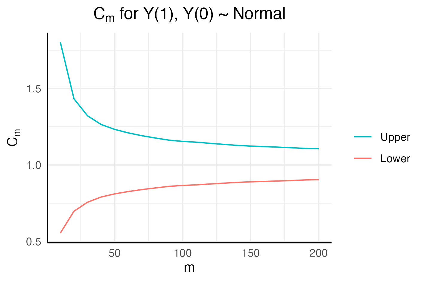
Figure 1: $C_{m}$ when $Y(1)\sim\mathcal{N}(\mu(1),\sigma^{2}(1))$ and $Y(0)\sim\mathcal{N}(\mu(0),\sigma^{2}(0))$. Monte Carlo integration using 10,000 draws.

We start with the toy model, where $Y(1)\sim\mathcal{N}(\mu(1),\sigma^{2}(1))$ and $Y(0)\sim\mathcal{N}(\mu(0),\sigma^{2}(0))$. Results are shown in Figure 1. The set of parameter values over which the FNA does worse is larger when $m$ is smaller. In fact, we show in Section 4 that if the data generating process (DGP) is sub-Gaussian, the length of $C_{m}$ is $O\left(m^{-1/2}\right)$. In the toy model, $C_{20}=[0.70,1.43]$, while $C_{50}$ is $[0.81,1.23]$. Suppose instead that $Y(1)\sim\mu(1)+\sigma(1)\chi^{2}_{1}$, $Y(0)\sim\mu(0)+\sigma(0)\chi^{2}_{1}$. Figure 2 shows that $C_{m}$ is wider across the range of $m$. In particular, $C_{20}=[0.49,2.22]$, while $C_{50}=[0.64,1.61]$. While the intervals may appear rather narrow at first glance, we provide numerous examples in Section 5 in which the amount of heteroskedasticity falls within this range.

Figure 2: $C_{m}$ when $Y(1)\sim\mu(1)+\sigma(1)\chi^{2}_{1}$ and $Y(0)\sim\mu(0)+\sigma(0)\chi^{2}_{1}$. Monte Carlo integration using 10,000 draws.

As our toy model shows, it is the estimation of $\widetilde{\sigma}(1)$ and $\widetilde{\sigma}(0)$ that causes problems when $m$ is small. It is therefore intuitive that $C_{m}$ will be wide when the distributions are fat tailed, that is, when kurtosis is high. As such, we consider the following parametrization: $Y(1)\sim\mu(1)+\sigma(1)\cdot\text{Pareto}(l,s)$ and $Y(0)\sim\mu(0)+\sigma(0)\cdot\text{Pareto}(l,s)$. Here, $l$ and $s$ are the location and scale parameters respectively. Figure 3 plots $C_{m}$ for $l=1$ and $s\in\{2,3,4\}$. Indeed, we see that the bands are much wider than in the previous models. For $s=2$, even when $m=100$, $C_{m}=[0.40,2.51]$, which, given the examples in Section 5 appear to be fairly extreme amounts of heteroskedasticity. Finally, we note that, $C_{m}$ decreases in width as we move from $s=2$ to $s=4$.

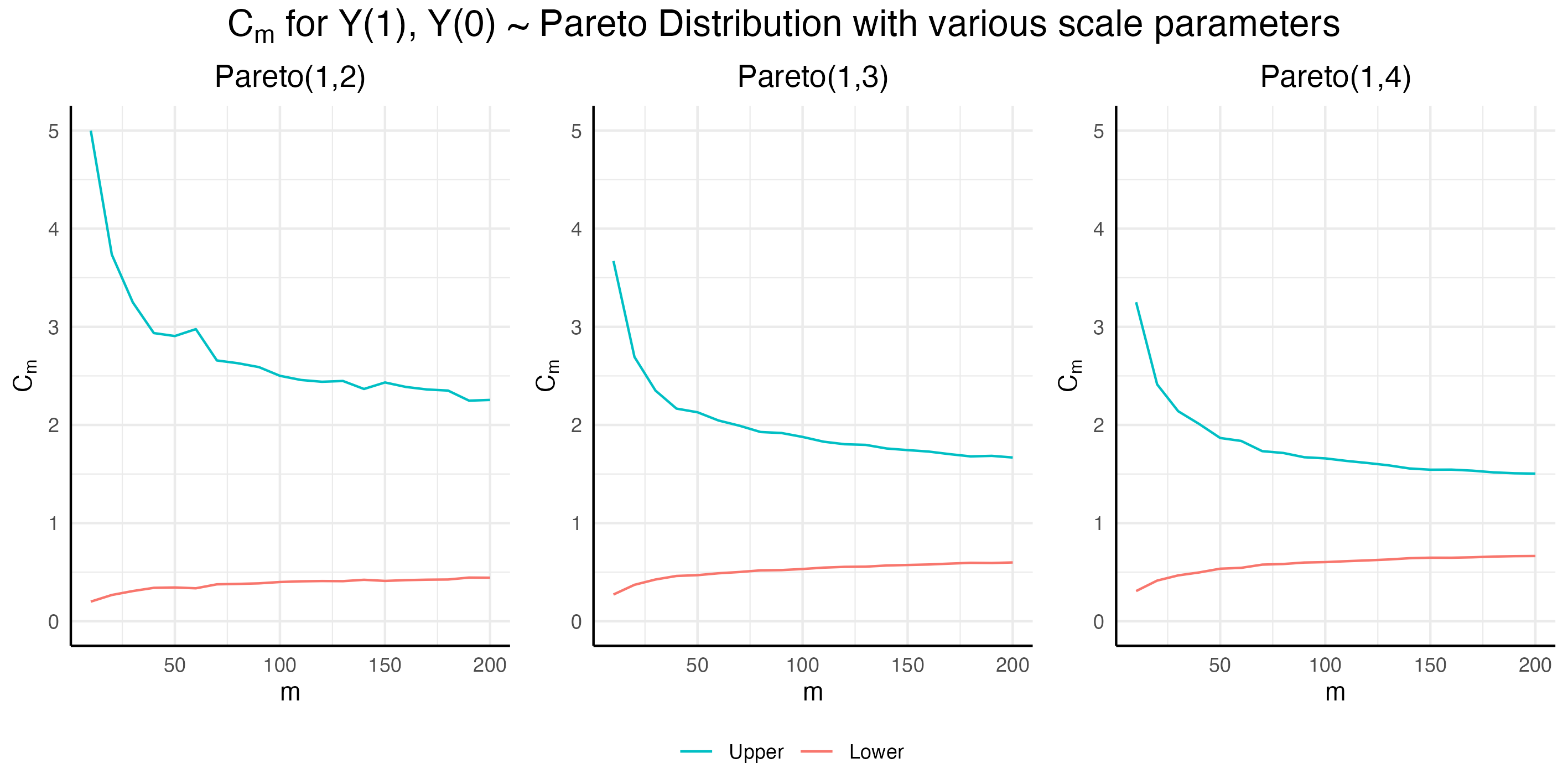
Figure 3: $C_{m}$ when $Y(1)\sim\mu(1)+\sigma(1)\cdot\text{Pareto}(1,s)$, $Y(0)\sim\mu(0)+\sigma(0)\cdot\text{Pareto}(1,s)$ and $s\in\{2,3,4\}$. Monte Carlo integration using 10,000 draws.

In sum, we see that the FNA does worse than the balanced allocation when the treatment and control groups are relatively homoskedastic. Furthermore, $C_{m}$ can be quite large when $m$ is small. The small pilot problem is exacerbated when observations exhibit cluster dependence, so that the “effective observations” are fewer in number. Small pilot issues can also arise when researchers perform stratified randomization with many strata, so that each stratum ends up with few observations. In Section 5, we argue that many empirical applications in fact have fairly homoskedastic outcomes. As such, unless a researcher has reason to believe that their outcomes are highly heteroskedastic, they should exercise caution in using the FNA with small pilots.

4 Theoretical Results

In this section, we study the theoretical properties of the FNA. We first review the case where $n,m\to\infty$. Next, we study the FNA in our asymptotic framework where $n\to\infty$ but $m$ is fixed, highlighting implications of our results for empirical researchers.

Large-$m$ asymptotics

Consider an asymptotic regime where both $m,n\to\infty$, corresponding to situations where both the pilot and the main wave are large. It is straightforward to show that $\widetilde{p}\overset{p}{\to}p_{*}$. Furthermore, we have that:

Proposition 4.1.

þ Under þLABEL:asm--2nd-moments,asm-1stwave-observation-process,asm-2ndwave-outcomes-device, as $m,n\to\infty$

$$\sqrt{n}\left(\widehat{\theta}_{\widetilde{p}}-\theta\right)\overset{d}{\to}\mathcal{N}\left(0,\Sigma_{\ast}\right),$$

where

$$\Sigma_{\ast}=\frac{\sigma^{2}(1)}{p_{\ast}}+\frac{\sigma^{2}(0)}{1-p_{\ast}}=(\sigma(1)+\sigma(0))^{2}.$$

In other words, $\widehat{\theta}_{\widetilde{p}}$ and $\widehat{\theta}_{p_{\ast}}$ have the same limiting distribution after suitable centering and scaling. This occurs because in the limit, noise coming from estimating $p_{*}$ with $\widetilde{p}$ is negligible in comparison to the sampling error of the difference-in-means estimator. Researchers employing the large $m$ framework essentially assume that $\widetilde{p}$ is an arbitrarily good estimator for $p_{*}$ so that its sampling error can be ignored. In practice, error in $\widetilde{p}$ can be large, particularly when $m$ is small. Asymptotic approximations that do not take this into account will likely perform poorly in finite sample.

Fixed-$m$ Asymptotics

To better understand the behavior of the FNA under small pilots, we study its properties in a novel asymptotic framework that takes $m$ to be fixed, even as $n\to\infty$.

A growing literature in econometrics uses fixed-sample asymptotics to study settings in which the “effective sample size” is small. For example, when data exhibit cluster-dependence, settings with few clusters pose unique challenges for estimation and inference. To tailor their analyses to these problems, papers such as [24], [11] and [12] employ asymptotic frameworks in which the number of clusters is fixed in the limit. Similarly, to model difference-in-differences studies involving few treated units, [15] keep the number of treated units fixed even as the number of untreated units tend to infinity. In the same vein, inference for regression discontinuity designs typically involves few observations around the discontinuity. To capture this, [10] analyze a permutation test under an asymptotic regime with a fixed number of observations on either side of the discontinuity.

Our approach is similar in spirit to these papers. In keeping $m$ fixed, we have that $\widetilde{p}$ is a noisy estimate of $p_{*}$ even in the limit. Preserving this important feature of the statistical problem makes our framework more appropriate for analyzing experiments with small pilots. In this setting, $\widehat{\theta}_{\widetilde{p}}$ converges in distribution to a mixture of Gaussians instead of $\mathcal{N}(0,\Sigma_{*})$. Furthermore, the form of the limiting mixture distribution depends on the distribution of $\widetilde{p}$. This is the content of the following proposition:

Proposition 4.2.

þ Under þLABEL:asm--2nd-moments,asm-1stwave-observation-process,asm-2ndwave-outcomes-device, if $m$ remains fixed as $n\to\infty$,

$$\sqrt{n}\left(\widehat{\theta}_{\widetilde{p}}-\theta\right)\overset{d}{\to}\mathcal{L}_{m}\leavevmode\nobreak\ ,$$

where $\mathcal{L}_{m}$ is a random variable whose distribution takes the form

$$\mathbb{P}\left(\mathcal{L}_{m}\leq t\right)=\int_{0}^{1}\Phi\left(\frac{t}{s\left(p\right)}\right)\;G_{m}(\mathrm{d}p),$$

$\Phi$ is the CDF of $\mathcal{N}(0,1)$, $G_{m}$ is the distribution of $\widetilde{p}$ and $s(\cdot)$ is defined by

$$s(p)=\sqrt{\frac{\sigma^{2}(1)}{p}+\frac{\sigma^{2}(0)}{1-p}}\ .$$

Remark 4.1.

þ The weak limit $\mathcal{L}_{m}$ in þ4.2 has mean zero. To see this, note that conditional on a value of the assignment probability $p$, i.e. conditional on the event $\widetilde{p}=p$, $\mathcal{L}_{m}$ has a $\mathcal{N}(0,s(p))$ distribution (where $s(p)$ is as defined in þ4.2). The conclusion then holds by the Law of Iterated Expectations.

To see the intuition for our result, recall that for each $p\in(0,1)$,

$$\sqrt{n}\left(\widehat{\theta}_{p}-\theta\right)\overset{d}{\to}\mathcal{N}\left(0,\frac{\sigma^{2}(1)}{p}+\frac{\sigma^{2}(0)}{1-p}\right)=\mathcal{N}\left(0,s^{2}(p)\right).$$

When $m$ is held fixed, in the limit as $n\to\infty$, $\widetilde{p}$ remains a non-degenerate random variable. In particular, the limiting distribution of $\widetilde{p}$ is its finite-sample distribution. Thus, the distribution of $\sqrt{n}\left(\widehat{\theta}_{\widetilde{p}}-\theta\right)$ becomes a mixture of the marginal distributions of the process

$$\left\{\sqrt{n}\left(\widehat{\theta}_{p}-\theta\right):p\in(0,1)\right\}\leavevmode\nobreak\ ,$$

where the mixing distribution is the distribution of $\widetilde{p}$, denoted here by $G_{m}$.

Implication for Experiments

Our results have implications for the use of the FNA when pilot sizes are small. In this sub-section we compare the asymptotic variances of $\widehat{\theta}_{\widetilde{p}}$, $\widehat{\theta}_{p_{\ast}}$ as well as $\widehat{\theta}_{p}$ with $p=\frac{1}{2}$. Since these estimators all have limit distributions that have mean zero (after centering around $\theta$ and scaling by $\sqrt{n}$), comparing asymptotic mean squared errors is equivalent to comparing the variances of the limit distributions. We first show that $\widehat{\theta}_{\widetilde{p}}$ has larger asymptotic variance in the fixed-$m$ regime than in the large-$m$ regime. We next show that under reasonable ranges of parameter values, the asymptotic variance of $\widehat{\theta}_{\widetilde{p}}$ can exceed that of $\widehat{\theta}_{p}$ with $p=\frac{1}{2}$.

Remark 4.2.

þ By þ4.2 and þ4.1, $\widehat{\theta}_{\widetilde{p}}$ has a limit distribution which has mean zero. Given that $\widehat{\theta}_{p_{\ast}}$ and $\widehat{\theta}_{p}$ also have mean zero normal limit distributions, comparing asymptotic mean squared errors is equivalent to comparing the variances of the limit distributions.

We begin with the corollary:

Corollary 4.3.

Under þLABEL:asm--2nd-moments,asm-1stwave-observation-process,asm-2ndwave-outcomes-device, suppose $m$ remains fixed as $n\to\infty$. $\mathcal{L}_{m}$ has variance:

$$\mathbb{E}\left[\frac{\sigma^{2}(1)}{\widetilde{p}}+\frac{\sigma^{2}(0)}{1-\widetilde{p}}\right]>\Sigma_{*}\leavevmode\nobreak\ .$$

In words, the asymptotic variance of $\widehat{\theta}_{\widetilde{p}}$ is larger under the fixed-$m$ regime than under the large-$m$ regime. When pilots are small, uncertainty in $\widetilde{p}$ may be large and could affect the asymptotic variance of $\widehat{\theta}_{\widetilde{p}}$. In particular, $\widehat{\theta}_{\widetilde{p}}$ will not be able to attain the optimal asymptotic variance of the infeasible allocation $p_{*}$. Conventional large-$m$ asymptotics may be too optimistic about the effectiveness of the Neyman Allocation with small pilots. We expect our analysis to better capture the behavior of $\widehat{\theta}_{\widetilde{p}}$ when pilots are small.

In addition to not attaining $\Sigma_{*}$, the $\widehat{\theta}_{\widetilde{p}}$ can do worse than $\widehat{\theta}_{p}$ for certain values of $\sigma^{2}(1)$ and $\sigma^{2}(0)$, as our next two results asserts. For convenience, define the following:

Definition 4.1.

Let $C_{m}$ be the set such that for a pilot of size $m$, $\widehat{\theta}_{\widetilde{p}}$ has higher asymptotic variance than $\widehat{\theta}_{p}$ if and only if $\frac{\sigma(1)}{\sigma(0)}\in C_{m}$. Let $|C_{m}|$ denote the length of $C_{m}$.

Definition 4.2.

Let

$$Z_{m}=\frac{\widetilde{\sigma}_{m}(1)}{\sigma(1)}\bigg{/}\frac{\widetilde{\sigma}_{m}(0)}{\sigma(0)}\leavevmode\nobreak\ .$$

and

$$B_{m}=\frac{1}{2}\,\mathbb{E}\left[\frac{1}{Z_{m}}+Z_{m}\right]\leavevmode\nobreak\ .$$

For our first result, we characterize the region $C_{m}$ in terms of $B_{m}$.

Proposition 4.4.

Under þLABEL:asm--2nd-moments,asm-1stwave-observation-process,asm-2ndwave-outcomes-device, suppose $m$ remains fixed as $n\to\infty$. Then

$$C_{m}=\left[\frac{1}{c_{m}}\,,\,c_{m}\right]\leavevmode\nobreak\ .$$ (4.1)

Furthermore,

$$c_{m}=B_{m}+\sqrt{B_{m}^{2}-1}>1\quad\text{and}\quad\left\lvert C_{m}\right\rvert=2\sqrt{B_{m}^{2}-1}\;>\;0\leavevmode\nobreak\ .$$

The properties of $C_{m}$ are intuitive. Firstly, $x\in C_{m}$ implies that $1/x\in C_{m}$. That is, the relative performance of the FNA to the balanced allocation does not change when we relabel treatment and control. Secondly, $1\in C_{m}$. This is because when ${\sigma(1)}/{\sigma(0)}=1$, the balanced allocation is optimal. Finally, note that $|C_{m}|$ depends on the bias of $\widetilde{\sigma}_{m}(1)/\widetilde{\sigma}_{m}(0)$ and $\widetilde{\sigma}_{m}(0)/\widetilde{\sigma}_{m}(1)$. In particular, if both terms are unbiased, $B_{m}=1$ and $|C_{m}|=0$. However, $\left\lvert C_{m}\right\rvert$ is strictly positive as long as $\widetilde{p}$ is not degenerate.

The exact properties of $C_{m}$ depends on the underlying distributions of potential outcomes. To understand its behavior in a more general setting, we study its first-order approximation. This yields the following:

Proposition 4.5.

Under þLABEL:asm--2nd-moments,asm-1stwave-observation-process,asm-2ndwave-outcomes-device, suppose $n\to\infty$. Suppose additionally that $Y_{i}(1)$ and $Y_{i}(0)$ are sub-Gaussian. Then,

$$C_{m}=\left[1-\sqrt{\frac{V}{m}}+\delta_{m}^{-}\,,\,1+\sqrt{\frac{V}{m}}+\delta_{m}^{+}\right]\leavevmode\nobreak\ ,$$

where $\delta_{m}^{+},\delta_{m}^{-}=o\left(\frac{1}{\sqrt{m}}\right)$ and

$$V=\frac{1}{4}\left(\frac{\mathbb{E}\left[\left(Y_{i}(1)-\mu(1)\right)^{4}\right]}{\sigma^{4}(1)}+\frac{\mathbb{E}\left[\left(Y_{i}(0)-\mu(0)\right)^{4}\right]}{\sigma^{4}(0)}-2\right)\leavevmode\nobreak\ .$$

Provided that the potential outcomes are sub-Gaussian, the relative efficiency of $\widehat{\theta}_{\widetilde{p}}$ and $\widehat{\theta}_{p}$ under $p=1/2$ is, to a first order, determined by the kurtosis of $Y_{i}(1)$ and $Y_{i}(0)$. Intuitively, if the potential outcomes have fatter tails, $\widetilde{p}$ will be poorly estimated, leading to larger variance in $\widehat{\theta}_{\widetilde{p}}$.

Furthermore, $|C_{m}|$ is shrinking to $0$ at the rate $1/\sqrt{m}$. Letting $m\to\infty$, $\widehat{\theta}_{\widetilde{p}}$ has weakly lower asymptotic variance across all parameter values. Hence, we recover the classic result concerning the optimality of the Neyman Allocation. When $m$ is small, however, $C_{m}$ can be wide, as Proposition 4.4 suggests. As we will argue in Section 5, many empirical applications have $\sigma(1)/\sigma(0)$ close to $1$, so that for small $m$, they fall within the range in which balanced randomization is preferred.

While the sub-Gaussian assumption limits the applicability of Proposition 4.5, it covers binary and bounded outcomes, which are relevant in empirical work. Furthermore, we consider it to be a negative result: even when potential outcomes are well-behaved, the FNA is sensitive to the kurtosis of the potential outcomes. It can still perform poorly relative to the balanced allocation as a result.

Remark 4.3.

Using an argument based on Taylor expansions, we can weaken the sub-Gaussian assumption to finiteness of the first $14^{\text{th}}$ moments. The proof is available on request.

5 Empirical Evidence of Approximate Homoskedasticity

To assess the amount of heteroskedasticity that empirical researchers face, we revisit the first 10 completed experiments in the AER RCT Registry. In each experiment, we ask the following question: Suppose the authors had access to a small pilot prior to the main study, would they have done better using the FNA instead of balanced randomization? In each experiment presented, we use the full experimental sample to estimate the standard deviations of each treatment arm and compute the corresponding ratios to see if these are close to one. In practice, researchers cannot do this given a small pilot since they do not have access to consistent variance estimators. Our findings suggest that these authors would likely not have not better with the FNA. We present two examples in this section: [2] is an experiment in which the outcomes are relatively homoskedastic. [1] contains outcome variables which are heteroskedastic. In this example, we also provide estimates of the interval $C_{m}$ and show that it will be wide even when $m$ is large. The remaining eight experiments are qualitatively similar to [2] and can be found in Section B.

5.1 [2]

There is a significant body of research examining the impact of school-level factors such as class size or teacher quality on educational performance of students. These are typically seen as the primary instruments for educational policy intervention. A large body of work also examines the impact of parental inputs on educational outcomes. [2] study whether or not parental inputs can be effectively manipulated through simple participation programs at schools. They do so via a large-scale randomized control trial in middle schools in the Créteil educational district of Paris. The experiment targeted families of 6th graders and the program consisted of a sequence of three meetings with parents every 2–3 weeks. The sessions focused on how parents can help their children by participating at school and at home in their education and additionally, included advice on how to adapt to results in end-of-term report cards. Participation in the program was randomized at the class level – half of the classes at a given school were assigned to the participation program. Classes are groups of 20–30 students. The overall sample comprised of 183 classes and a total of 4,308 students. The study tracked three types of outcomes: (1) parental involvement attitudes and behaviour; (2) children’s behaviour, namely truancy, disciplinary record and work effort; and (3) children’s academic results. Since randomization was done at the class-level, we examine heteroskedasticity with respect to treatment status at both the individual level and at the class level.

Table 1 reports student-level standard deviations in treatment and control groups, as well as their ratios, for the main outcomes of interest. These are the outcomes considered in Tables 2, 3 and 5 in [2]. The ratios are all close to one, so that by and large the treatment and control groups are relatively homoskedastic at the student level. This indicates that if the experimenters were to run a randomized control trial in the same population with treatment assigned at the individual-level, the FNA would likely yield no improvement relative to the balanced allocation.

Table 2 reports standard deviations and their ratios in class-level means of outcomes. This corresponds to a scenario in which classes are the units of interest, with class-level means as the relevant outcomes. We first calculate class-level means and then compute their standard deviations across classes for the treatment and control groups respectively. The standard deviation ratios for class-level means are by and large also close to one. Hence, if the hypothetical experiment was to be conducted at the class-level, the treatment and control groups would still be relatively homoskedastic. In this case, the FNA would again not improve upon the balanced allocation.

Table 1: Student-Level Heteroskedasticity in [2].

Outcome Variables		Treatment	Control	Treat./Cont.
Parental Involvement	Global parenting score	0.34	0.34	1.01
	School-based involvement score	0.66	0.63	1.05
	Home-based involvement score	0.59	0.57	1.04
	Understanding and perceptions score	0.53	0.55	0.97
	Parent-school interaction	0.40	0.40	1.01
	Parental monitoring of school work	0.43	0.41	1.05
Behavior	Absenteeism	6.29	8.63	0.73
	Pedagogical team: Behavioral score	0.73	0.74	0.98
	Pedagogical team: Discipl. sanctions	1.20	1.18	1.02
	Pedagogical team: Good conduct	0.49	0.47	1.04
	Pedagogical team: Honors	0.28	0.32	0.89
	Teacher assessment: Behavior in class	0.48	0.49	0.98
	Teacher assessment: School work	0.49	0.50	1.00
Test Scores	French (Class grade)	3.73	3.70	1.01
	Mathematics (Class grade)	4.26	4.25	1.00
	Average across subjects (Class grade)	2.87	2.88	1.00
	Progress over the school year	0.49	0.49	0.99
	French (Uniform test)	0.99	1.01	0.98
	Mathematics (Uniform test)	0.99	1.02	0.98

Table 2: Class-Level Heteroskedasticity in [2].

Outcome Variables		Treatment	Control	Treat./Cont.
Parental Involvement	Global parenting score	0.12	0.12	0.97
	School-based involvement score	0.24	0.35	0.69
	Home-based involvement score	0.20	0.15	1.33
	Understanding and perceptions score	0.20	0.22	0.94
	Parent-school interaction	0.13	0.12	1.09
	Parental monitoring of school work	0.13	0.14	0.96
Behavior	Absenteeism	2.21	3.45	0.64
	Pedagogical team: Behavioral score	0.24	0.27	0.88
	Pedagogical team: Discipl. sanctions	0.36	0.36	1.01
	Pedagogical team: Good conduct	0.22	0.23	0.95
	Pedagogical team: Honors	0.10	0.11	0.87
	Teacher assessment: Behavior in class	0.16	0.16	1.01
	Teacher assessment: School work	0.15	0.14	1.02
Test Scores	French (Class grade)	1.32	1.31	1.01
	Mathematics (Class grade)	1.76	1.84	0.96
	Average across subjects (Class grade)	0.83	0.93	0.89
	Progress over the school year	0.16	0.14	1.11
	French (Uniform test)	0.42	0.42	1.01
	Mathematics (Uniform test)	0.40	0.43	0.93

5.2 [1]

A large body of economic models posit that individuals have time inconsistent preferences, exhibiting more impatience for near-term trade-offs than for future trade-offs. The implication of these models is that those who engage in commitment devices ex ante may improve their welfare. To test this hypothesis, [1] conducted an RCT in the Philippines, in which individuals were offered randomly offered the chance to open a SEED (Save, Earn, Enjoy Deposits) account. Money deposited into the account cannot be withdrawn until the owner reached a goal, such as reaching a savings amount or until a pre-specified month in which they expected large expenditures.

Partnering with a rural bank in Mindanao, they authors surveyed 1,777 of their existing or former clients, of which 842 were placed into the treatment group, while 469 were placed in the control group. As treatment involved receiving a briefing on the importance of savings, the remaining 466 individuals were placed in the marketing group, receiving the briefing but not access to SEED. We focus on the Table VI of [1], containing results on saving behavior. The parameter of interest is the Intent-to-Treat effect, with approximately 25% of the treated taking up treatment. Here, the authors find that relative to the control group, the treatment group had a higher change in savings 6 months (6m) and 12 months (12m) after treatment. Comparing treatment to marketing group led to weaker but still positive results.

We present standard deviations of the outcomes as well as their ratios in Table 3. We first note that Change in Balance $>0\%$ (12m) and Change in Balance $>20\%$ (12m) are binary variables which are relatively homoskedastic. Change in Total Balance (6m) and Change in Total Balance (12m), measured in Philippine pesos, exhibit more heteroskedasticity. In particular, comparing the treatment group to the marketing group at the 12 month period, we observe a standard deviation ratio of $3.13$. At first glance, this suggests that the FNA might outperform balanced randomization, at least with respect to this specific outcome. This turns out to be false once we investigate the heteroskedasticity in Change in Total Balance (6m) and Change in Total Balance (12m). Quantiles of these variables are displayed in Table 4. Clearly, they have extremely fat right tails, which we confirm by computing the kurtosis, contained in Table 5. Fat tails worsen the performance of a variety of statistical techniques, including the FNA, as our analysis in Section 4 shows.

Table 3: Heteroskedasticity in [1]

	Treat.	Cont.	Market.	Treat./Cont.	Treat./Market.
Change in Tot. Bal. (6m)	2347.60	2880.70	1335.98	1.76	0.81
Change in Tot. Bal. (12m)	6093.24	1945.00	2690.65	2.26	3.13
Change in Tot. Bal. $>$ 0% (12m)	0.47	0.45	0.42	1.11	1.05
Change in Tot. Bal. $>$ 20% (12m)	0.40	0.35	0.31	1.30	1.16

Table 4: Quantiles of Outcome Variables in [1].

Variable	Group	1%	5%	10%	50%	90%	95%	99%	99.5%	99.9%
Change Tot. Bal. (6m)	Treat.	-1100	-500	-300	0	500	1500	7200	13100	28900
	Market.	-1000	-600	-400	0	100	900	5600	12200	40800
	Cont.	-1600	-600	-500	0	0	600	2700	6100	18400
Change Tot. Bal. (12m)	Treat.	-1300	-900	-500	0	500	1600	8500	18100	102300
	Market.	-1300	-900	-500	-100	300	1600	10500	15700	19900
	Cont.	-2000	-1200	-800	-100	100	900	6500	8100	34300

Table 5: Kurtosis of the Outcome Variables in [1]

Variable	Treat.	Market.	Cont.
Change in Tot. Bal. (6m)	252.78	218.92	156.33
Change in Tot. Bal. (12m)	258.56	66.56	309.89

Researchers cannot estimate $C_{m}$ if the only have access to a small pilot. However, using the full experiment data, we are able to estimate $C_{m}$ for a range of $m$. Our results are displayed in Figure 4. Given the high kurtosis, there is a relatively large range of ratios of standard deviations for which the balanced allocation is preferred to the FNA. We can further compute the $m$ necessary before the FNA outperforms the balanced allocation. Our results are collected in Table 6. The first two rows, labelled “Exact”, refer to intervals which are computed using the full experiment. Here, we see that the necessary pilot sizes are between 25–50% of the full experiment. For the comparison of Treatment and Marketing group at 6 months, the necessary pilot size exceeds $2,000$, falling outside the set of grid points we explored. To complete the analysis, we use our asymptotic result to obtain approximations of the necessary $m$. Comparing the asymptotic intervals to the exact ones, we see that the former is far too optimistic for the fat-tailed DGP in [1]. This is likely because the sub-Gaussian assumption is inappropriate for this data. Nonetheless, applying the asymptotic bounds to the case of Treatment vs Marketing group at 6 months, we find that a pilot size of 7,000 would be necessary for the FNA to outperform balanced randomization. This is nearly 4 times the size of the actual experiment.

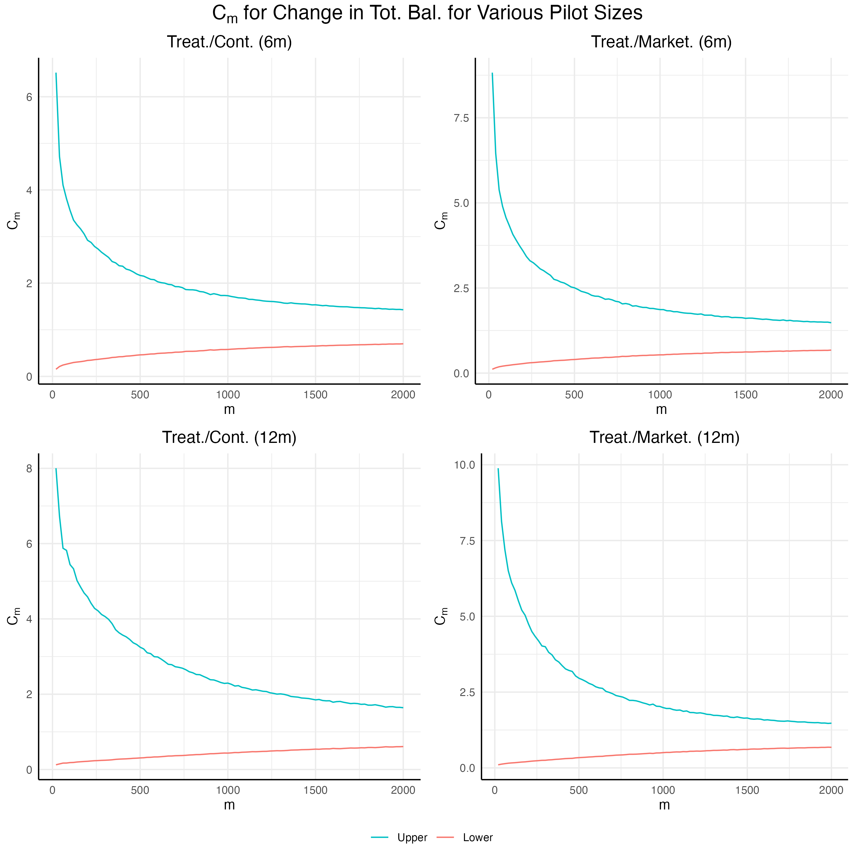
Figure 4: $C_{m}$ for the outcomes of interest estimated using the full experiment data. Interval computed under the assumption that the pilot assigns half of the units to treatment and half to control.

Table 6: Necessary Pilot Sizes

	Treat./Cont.	Treat./Market.
Exact 6m	930.70	–
Exact 12m	1014.94	475.29
Asympt. 6m	355.02	6857.59
Asympt. 12m	177.10	35.52

In sum, our analysis suggests that the FNA would have performed poorly in the context of [1]. Even though the outcomes of interest exhibit stronger heteroskedasticity, the fat tails of the outcome distributions also impedes the estimation of $\widetilde{p}$, so that ultimately, very large pilot sizes are needed for the FNA to outperform the balanced allocation in this example.

6 Conclusion

We study the properties of the Feasible Neyman Allocation (FNA) in a novel asymptotic framework for two-wave experiments that takes pilot size to be fixed as the size of the main wave tends to infinity. In this setting, the estimated allocation has error that is not negligible even in the limit. Our asymptotic model therefore corresponds more closely to the finite sample statistical problem when pilots are small and the optimal allocation may be poorly estimated. We establish the limiting distribution of the difference-in-means estimator under the FNA and characterize conditions under which it has larger asymptotic variance compared to balanced randomization, where half of the main wave is assigned to treatment and the remainder to control. This happens when the potential outcomes are relatively homoskedastic with respect to treatment status or exhibit high kurtosis – situations that may arise frequently in practice. This issue is likely to be exacerbated when observations exhibit cluster dependence or when researchers perform stratified randomization with many strata, so that the “effective observations” used for variance computations are fewer in number. Our results suggest that researchers should not use the FNA with small pilots, particularly when they believe any of the above occurs.

Appendix A Proofs

A.1 Proofs of Propositions 4.1, 4.2

A.1.1 Some preliminaries and common machinery for the proofs

Our proofs in this section require some common machinery. Let $\left\{\left(Y_{i}^{\ast}(0),Y_{i}^{\ast}(1)\right)\right\}_{i=1}^{\infty}$ be i.i.d. random vectors with distribution equal to that of $(Y(0)-\mu(0),Y(1)-\mu(1))$ that satisfy

$$\left\{\left(Y_{i}^{\ast}(0),Y_{i}^{\ast}(1)\right)\right\}_{i=1}^{\infty}\raisebox{0.50003pt}{\rotatebox[origin={c}]{90.0}{$\models$}}\left\{\left\{\widetilde{Y}_{i}(0),\widetilde{Y}_{i}(1),\widetilde{A}_{i}\right\}_{i=1}^{\infty},\left\{Y_{i}(0),Y_{i}(1),U_{i}\right\}_{i=1}^{\infty}\right\}.$$

þA.3 provides detailed arguments showing that

$$\sqrt{n}\left(\widehat{\theta}_{\widetilde{p}}-\theta\right)\overset{d}{=}\frac{\frac{1}{\sqrt{n}}\sum_{i=1}^{n\overline{A}_{\widetilde{p}}}Y_{i}^{\ast}(1)}{\overline{A}_{\widetilde{p}}}-\frac{\frac{1}{\sqrt{n}}\sum_{i=n\overline{A}_{\widetilde{p}}+1}^{n}Y_{i}^{\ast}(0)}{1-\overline{A}_{\widetilde{p}}}.$$ (A.1)

Consider the partial-sums process

$$\mathbf{T}_{n}(u)=\left(\begin{array}[]{c}T_{n}(0,u)\\ T_{n}(1,u)\end{array}\right)=\frac{1}{\sqrt{n}}\sum_{i=1}^{\left\lfloor u\cdot n\right\rfloor}\left(\begin{array}[]{c}Y_{i}^{\ast}(0)\\ Y_{i}^{\ast}(1)\end{array}\right)\qquad\forall u\in[0,1]$$ (A.2)

By hypothesis, $\left\{\left(Y_{i}^{\ast}(0),Y_{i}^{\ast}(1)\right)\right\}_{i=1}^{\infty}$ are mean zero, have finite variance and are i.i.d. across $i\in\mathbb{N}$. Denote the space of all essentially bounded functions on $[0,1]$ endowed with the essential supremum norm by $\ell^{\infty}([0,1])$. By a two-dimensional variant of Donsker’s Functional Central Limit Theorem (see for instance [33, Theorem 4.3.5 ]), $\mathbf{T}_{n}^{\ast}(\cdot)$ converges weakly in $\ell^{\infty}([0,1])^{2}$ to a two-dimensional scaled Brownian motion $\mathbf{T}_{\infty}(\cdot)$

$$\mathbf{T}_{\infty}(u)=\left(\begin{array}[]{c}T_{\infty}(u,0)\\ T_{\infty}(u,1)\end{array}\right)=\Sigma^{\frac{1}{2}}B(u)\qquad\forall u\in[0,1]$$ (A.3)

where $B(\cdot)$ is a two-dimensional standard Brownian motion and $\Sigma^{\frac{1}{2}}$ is the unique symmetric matrix satisfying $\Sigma=\left(\Sigma^{\frac{1}{2}}\right)^{\prime}\Sigma^{\frac{1}{2}}$. We can write the vector comprised of the numerators in (A.1) as

$$U_{n}=\left(\begin{array}[]{c}\frac{1}{\sqrt{n}}\sum_{i=1}^{n\overline{A}_{\widetilde{p}}}Y_{i}^{\ast}(1)\\ \frac{1}{\sqrt{n}}\sum_{i=n\overline{A}_{\widetilde{p}}+1}^{n}Y_{i}^{\ast}(0)\end{array}\right)=\left(\begin{array}[]{c}T_{n}\left(1,\overline{A}_{\widetilde{p}}\right)\\ T_{n}(0,1)-T_{n}\left(0,\overline{A}_{\widetilde{p}}\right)\end{array}\right)$$ (A.4)

so that by (A.1),

$$\sqrt{n}\left(\widehat{\theta}_{\widetilde{p}}-\theta\right)\overset{d}{=}\left[\begin{array}[]{cc}\frac{1}{\overline{A}_{\widetilde{p}}},&-\frac{1}{1-\overline{A}_{\widetilde{p}}}\end{array}\right]\cdot U_{n}\ .$$ (A.5)

A.1.2 Proof of Proposition 4.1

Proof of þ4.1.

By þA.2, $\overline{A}_{\widetilde{p}}\overset{\mathrm{a.s.}}{\to}p_{\ast}$ as $m,n\to\infty$. Furthermore, [32] Theorems 18.10 (v) and 18.11 imply that $U_{n}$ in (A.4) satisfies

$$U_{n}\overset{d}{\to}U:=\left(\begin{array}[]{c}T_{\infty}\left(1,p_{\ast}\right)\\ T_{\infty}\left(0,1\right)-T_{\infty}\left(0,p_{\ast}\right)\end{array}\right)\sim\mathcal{N}\left(\left(\begin{array}[]{c}0\\ 0\end{array}\right),\left(\begin{array}[]{cc}p_{\ast}\cdot\sigma^{2}(1)&0\\ 0&\left(1-p_{\ast}\right)\cdot\sigma^{2}(0)\end{array}\right)\right).$$ (A.12)

where the covariance matrix is derived using the fact that a standard Brownian motion has independent increments. By (A.12), $\overline{A}_{\widetilde{p}}\overset{\mathrm{a.s.}}{\to}p_{\ast}$ and Slutsky’s Theorem, as $m,n\to\infty$,

$$\sqrt{n}\left(\widehat{\theta}_{\widetilde{p}}-\theta\right)\overset{d}{=} \ \frac{\frac{1}{\sqrt{n}}\sum_{i=1}^{n\overline{A}_{\widetilde{p}}}Y_{i}^{\ast}(1)}{\overline{A}_{\widetilde{p}}}-\frac{\frac{1}{\sqrt{n}}\sum_{i=n\overline{A}_{\widetilde{p}}+1}^{n}Y_{i}^{\ast}(0)}{1-\overline{A}_{\widetilde{p}}}$$

$$= \ \left[\begin{array}[]{cc}\frac{1}{\overline{A}_{\widetilde{p}}}&-\frac{1}{1-\overline{A}_{\widetilde{p}}}\end{array}\right]\cdot U_{n}$$

$$\overset{d}{\to} \ \left[\begin{array}[]{cc}\frac{1}{p_{\ast}}&-\frac{1}{1-p_{\ast}}\end{array}\right]\cdot U$$

$$\sim \ \mathcal{N}\left(0,\frac{\sigma^{2}(1)}{p_{\ast}}+\frac{\sigma^{2}(0)}{1-p_{\ast}}\right).$$

∎

A.1.3 Proof of Proposition 4.2

Proof of þ4.2.

Note that the process $\mathbf{T}_{n}$ in (A.2) is independent to $\overline{A}_{\widetilde{p}}$ for every $n\in\mathbb{N}$. Additionally, $\overline{A}_{\widetilde{p}}\overset{\mathrm{p}}{\to}\widetilde{p}$ (by þA.2) and $\mathbf{T}_{n}\overset{\mathrm{d}}{\to}\mathbf{T}_{\infty}$ as $n\to\infty$, where $\overset{\mathrm{d}}{\to}$ denotes weak convergence in $\ell^{\infty}([0,1])^{2}$. This implies that (see for instance [31, Example 1.4.6 ])

$$\left(\begin{array}[]{c}\overline{A}_{\widetilde{p}}\\ \mathbf{T}_{n}(\cdot)\end{array}\right)\overset{\mathrm{d}}{\to}\left(\begin{array}[]{c}\widetilde{p}\\ \mathbf{T}_{\infty}(\cdot)\end{array}\right)\qquad\text{as }n\to\infty$$ (A.13)

where $\widetilde{p}$ and $\mathbf{T}_{\infty}$ are independent and $\overset{\mathrm{d}}{\to}$ is in the sense of weak convergence in $[0,1]\times\ell^{\infty}([0,1])^{2}$. Equation (A.13) alongside þA.5 and [32] Theorem 18.11 imply that in this case, as $n\to\infty$, $U_{n}$ in equation (A.4)

$$U_{n}\overset{\mathrm{d}}{\to}\widetilde{U}:=\left(\begin{array}[]{c}T_{\infty}\left(1,\widetilde{p}\right)\\ T_{\infty}(0,1)-T_{\infty}\left(0,\widetilde{p}\right).\end{array}\right)$$ (A.14)

We should note that measurability of $\widetilde{U}$ is derived in þA.6. Using (A.5) in combination with (A.14), we get

$$\sqrt{n}\left(\widehat{\theta}_{\widetilde{p}}-\theta\right)\overset{\mathrm{d}}{=} \ \left[\begin{array}[]{cc}\frac{1}{\overline{A}_{\widetilde{p}}}&-\frac{1}{1-\overline{A}_{\widetilde{p}}}\end{array}\right]\cdot U_{n}$$

$$\overset{\mathrm{d}}{\to} \ \left[\begin{array}[]{cc}\frac{1}{\widetilde{p}}&-\frac{1}{1-\widetilde{p}}\end{array}\right]\cdot\widetilde{U}$$

$$= \ \frac{1}{\widetilde{p}}T_{\infty}\left(1,\widetilde{p}\right)-\frac{1}{1-\widetilde{p}}\left[T_{\infty}(0,1)-T_{\infty}\left(0,\widetilde{p}\right)\right]$$

$$=: \ \mathcal{L}_{m}.$$

The distribution of $\mathcal{L}_{m}$ can be derived as a corollary of þA.6, but we include the direct derivation here for completeness. To derive the distribution of $\mathcal{L}_{m}$ in closed form, notice that $\mathcal{L}_{m}|\widetilde{p}\sim\mathcal{N}\left(0,\frac{\sigma^{2}(1)}{\widetilde{p}}+\frac{\sigma^{2}(0)}{1-\widetilde{p}}\right)$ so that

$$\mathbb{P}\left(\mathcal{L}_{m}\leq t\middle|\widetilde{p}\right)=\Phi\left(\frac{t}{s\left(\widetilde{p}\right)}\right)\qquad\text{where }s^{2}\left(\widetilde{p}\right)=\frac{\sigma^{2}(1)}{\widetilde{p}}+\frac{\sigma^{2}(0)}{1-\widetilde{p}}.$$

By the Law of Total Probability, it follows that

$$\mathbb{P}\left(\mathcal{L}_{m}\leq t\right)=\int_{0}^{1}\Phi\left(\frac{t}{s\left(p\right)}\right)\;G_{m}(\mathrm{d}p),$$

where $G_{m}(\cdot)$ is the distribution of $\widetilde{p}$. ∎

A.1.4 Auxiliary lemmas

Lemma A.1.

þ Suppose þ2.2 holds and additionally that, there is some $p_{1}\in(0,1)$ such that $\frac{1}{m}\sum_{i=1}^{m}\widetilde{A}_{i}\overset{\mathrm{p}}{\to}\mathbb{P}\left(\widetilde{A}_{1}=1\right)=p_{1}$ as $m\to\infty$. Then $\widetilde{p}\overset{\mathrm{p}}{\to}p_{\ast}$ as $m\to\infty$.

Proof.

Let $a\in\{0,1\}$ be given. Note that for any Borel function $h:\mathbb{R}\to\mathbb{R}$ with $\mathbb{E}[|h(Y(a))|]<\infty$, as $m\to\infty$,

$$\frac{1}{m}\sum_{i=1}^{m}h\left(\widetilde{Y}_{i}\right)\mathbb{I}\left\{\widetilde{A}_{i}=a\right\}=\frac{1}{m}\sum_{i=1}^{m}h\left(\widetilde{Y}_{i}(a)\right)\mathbb{I}\left\{\widetilde{A}_{i}=a\right\}\overset{\mathrm{a.s.}}{\to}\mathbb{E}\left[h\left(\widetilde{Y}_{1}(a)\right)\mathbb{I}\left\{\widetilde{A}_{1}=a\right\}\right]$$

Under þ2.2, $\widetilde{Y}_{1}(a)\raisebox{0.50003pt}{\rotatebox[origin={c}]{90.0}{$\models$}}\widetilde{A}_{1}$ and $\widetilde{Y}_{1}(a)\sim Y(a)$ so that,

$$\frac{1}{m}\sum_{i=1}^{m}h\left(\widetilde{Y}_{i}\right)\mathbb{I}\left\{\widetilde{A}_{i}=a\right\}\overset{\mathrm{a.s.}}{\to}\mathbb{E}\left[h(Y(a))\right]\cdot p_{1}^{a}\cdot\left(1-p_{1}\right)^{1-a}\quad\text{as }m\to\infty$$

The hypothesis of the question gives us that $\frac{1}{m}\sum_{i=1}^{m}\mathbb{I}\left\{\widetilde{A}_{i}=a\right\}\overset{\mathrm{p}}{\to}p_{1}^{a}\cdot\left(1-p_{1}\right)^{1-a}\in(0,1)$. Thus, by the Continuous Mapping Theorem, as $m\to\infty$

$$\frac{\frac{1}{m}\sum_{i=1}^{m}h\left(\widetilde{Y}_{i}\right)\mathbb{I}\left\{\widetilde{A}_{i}=a\right\}}{\frac{1}{m}\sum_{i=1}^{m}\mathbb{I}\left\{\widetilde{A}_{i}=a\right\}}\overset{\mathrm{a.s.}}{\to}\mathbb{E}\left[h(Y(a))\right]$$

Setting $h$ equal to the maps $y\mapsto y$ and $y\mapsto y^{2}$, we get respectively that

$$\begin{split}\frac{\frac{1}{m}\sum_{i=1}^{m}\widetilde{Y}_{i}\mathbb{I}\left\{\widetilde{A}_{i}=a\right\}}{\frac{1}{m}\sum_{i=1}^{m}\mathbb{I}\left\{\widetilde{A}_{i}=a\right\}}\overset{\mathrm{p}}{\to}&\ \mathbb{E}[Y(a)]\\ \frac{\frac{1}{m}\sum_{i=1}^{m}\widetilde{Y}_{i}^{2}\mathbb{I}\left\{\widetilde{A}_{i}=a\right\}}{\frac{1}{m}\sum_{i=1}^{m}\mathbb{I}\left\{\widetilde{A}_{i}=a\right\}}\overset{\mathrm{p}}{\to}&\ \mathbb{E}\left[Y(a)^{2}\right]\end{split}$$

Combining these with the Continuous Mapping Theorem again, it follows that as $m\to\infty$

$$\widetilde{\sigma}_{m}^{2}(a)= \ \frac{1}{\sum_{i=1}^{m}\mathbb{I}\left\{\widetilde{A}_{i}=a\right\}-1}\sum_{i=1}^{m}\left(\widetilde{Y}_{i}\mathbb{I}\left\{\widetilde{A}_{i}=a\right\}-\frac{1}{\sum_{i=1}^{m}\mathbb{I}\left\{\widetilde{A}_{i}=a\right\}}\sum_{i=1}^{m}\widetilde{Y}_{i}\mathbb{I}\left\{\widetilde{A}_{i}=a\right\}\right)^{2}$$

$$\overset{\mathrm{p}}{\to} \ \sigma^{2}(a)$$

By another application of the Continuous Mapping Theorem,

$$\widetilde{p}=\frac{\widetilde{\sigma}_{m}(1)}{\widetilde{\sigma}_{m}(1)+\widetilde{\sigma}_{m}(0)}\overset{\mathrm{p}}{\to}\frac{\sigma(1)}{\sigma(1)+\sigma(0)}=p_{\ast}.$$

∎

Lemma A.2.

þ Let $\overline{A}_{\widetilde{p}}=\frac{1}{n}\sum_{i=1}^{n}A_{\widetilde{p},i}$. Under þ2.2, þ2.3 and equation (2.3), and fixed $m\in\mathbb{N}$, $\overline{A}_{\widetilde{p}}\overset{\mathrm{p}}{\to}\widetilde{p}$ as $n\to\infty$. Additionally, $\overline{A}_{\widetilde{p}}\overset{\mathrm{p}}{\to}p_{\ast}$ as $m,n\to\infty$.

Proof.

Note that given any fixed $m\in\mathbb{N}$, $A_{\widetilde{p},i}|\widetilde{p}\sim\mathrm{Bernoulli}\left(\widetilde{p}\right)$ independently across $i\in\mathbb{N}$. By De Finetti’s Theorem, $\left\{A_{\widetilde{p},i}\right\}_{i=1}^{\infty}$ forms an exchangeable sequence of random variables. By the Strong Law of Large Numbers for exchangeable sequences (see for instance [29, Theorem 1.62 ] or [25]), it follows that $\overline{A}_{\widetilde{p}}\overset{\mathrm{a.s.}}{\to}\widetilde{p}$ as $n\to\infty$. Next, we consider the case with both $m,n\to\infty$. Using the triangle inequality,

$$\left|\overline{A}_{\widetilde{p}}-p_{\ast}\right|\leq\left|\overline{A}_{\widetilde{p}}-\widetilde{p}\right|+\left|\widetilde{p}-p_{\ast}\right|\leq\sup_{p\in[0,1]}\left|\frac{1}{n}\sum_{i=1}^{n}\mathbb{I}\left\{U_{i}\leq p\right\}-p\right|+\left|\widetilde{p}-p_{\ast}\right|.$$

By þA.1, $\left|\widetilde{p}-p_{\ast}\right|\overset{\mathrm{p}}{\to}0$ as $m\to\infty$. An immediate consequence of the Glivenko-Cantelli Theorem is that $\sup_{p\in[0,1]}\left|\frac{1}{n}\sum_{i=1}^{n}\mathbb{I}\left\{U_{i}\leq p\right\}-p\right|\overset{\mathrm{a.s.}}{\to}0$ as $n\to\infty$. ∎

Lemma A.3.

þ Under þ2.2, þ2.3 and equation (2.3), we can write

$$\sqrt{n}\left(\widehat{\theta}_{\widetilde{p}}-\theta\right)\overset{\mathrm{d}}{=}\frac{\frac{1}{\sqrt{n}}\sum_{i=1}^{n\overline{A}_{\widetilde{p}}}Y_{i}^{\ast}(1)}{\overline{A}_{\widetilde{p}}}-\frac{\frac{1}{\sqrt{n}}\sum_{i=n\overline{A}_{\widetilde{p}}+1}^{n}Y_{i}^{\ast}(0)}{1-\overline{A}_{\widetilde{p}}}$$

where $\left\{\left(Y_{i}^{\ast}(0),Y_{i}^{\ast}(1)\right)\right\}_{i=1}^{\infty}$ are i.i.d. random vectors with distribution equal to that of $(Y(0)-\mu(0),Y(1)-\mu(1))$ and

$$\left\{\left(Y_{i}^{\ast}(0),Y_{i}^{\ast}(1)\right)\right\}_{i=1}^{\infty}\raisebox{0.50003pt}{\rotatebox[origin={c}]{90.0}{$\models$}}\left\{\left\{\widetilde{Y}_{i}(0),\widetilde{Y}_{i}(1),\widetilde{A}_{i}\right\}_{i=1}^{\infty},\left\{Y_{i}(0),Y_{i}(1),U_{i}\right\}_{i=1}^{\infty}\right\}.$$ (A.15)

Proof.

We can rewrite $\widehat{\theta}_{\widetilde{p}}$ using the potential outcomes as is standard:

$$\widehat{\theta}_{\widetilde{p}}=\frac{\frac{1}{n}\sum_{i=1}^{n}Y_{i}(1)A_{\widetilde{p},i}}{\overline{A}_{\widetilde{p}}}-\frac{\frac{1}{n}\sum_{i=1}^{n}Y_{i}(0)\left(1-A_{\widetilde{p},i}\right)}{1-\overline{A}_{\widetilde{p}}}.$$

where $\overline{A}_{\widetilde{p}}=\frac{1}{n}\sum_{i=1}^{n}A_{\widetilde{p},i}$. Furthermore, since $\theta=\mu(1)-\mu(0)$,

$$\widehat{\theta}_{\widetilde{p}}-\theta= \ \left(\frac{\frac{1}{n}\sum_{i=1}^{n}Y_{i}(1)A_{\widetilde{p},i}}{\overline{A}_{\widetilde{p}}}-\mu(1)\right)-\left(\frac{\frac{1}{n}\sum_{i=1}^{n}Y_{i}(0)\left(1-A_{\widetilde{p},i}\right)}{1-\overline{A}_{\widetilde{p}}}-\mu(0)\right)$$

$$= \ \frac{\frac{1}{n}\sum_{i=1}^{n}\left[Y_{i}(1)-\mu(1)\right]A_{\widetilde{p},i}}{\overline{A}_{\widetilde{p}}}-\frac{\frac{1}{n}\sum_{i=1}^{n}\left[Y_{i}(0)-\mu(0)\right]\left(1-A_{\widetilde{p},i}\right)}{1-\overline{A}_{\widetilde{p}}}.$$

Thus,

$$\sqrt{n}\left(\widehat{\theta}_{\widetilde{p}}-\theta\right)=\frac{\frac{1}{\sqrt{n}}\sum_{i=1}^{n}\left[Y_{i}(1)-\mu(1)\right]A_{\widetilde{p},i}}{\overline{A}_{\widetilde{p}}}-\frac{\frac{1}{\sqrt{n}}\sum_{i=1}^{n}\left[Y_{i}(0)-\mu(0)\right]\left(1-A_{\widetilde{p},i}\right)}{1-\overline{A}_{\widetilde{p}}}.$$

Note that the distribution $\sqrt{n}\left(\widehat{\theta}_{\widetilde{p}}-\theta\right)$ is invariant to permutation of the sample indices. Hence the distribution of $\sqrt{n}\left(\widehat{\theta}_{\widetilde{p}}-\theta\right)$ does not change if we reorder the sample indices to have $i=1,\dots,n\overline{A}_{\widetilde{p}}$ correspond to the observations in the treatment group and $i=n\overline{A}_{\widetilde{p}}+1,\dots,n$ correspond to the observations in the control group. Notice also, that under þ2.2, þ2.3, and (A.15), the resulting permuted sum has the same distribution as

$$\frac{\frac{1}{\sqrt{n}}\sum_{i=1}^{n\overline{A}_{\widetilde{p}}}Y_{i}^{\ast}(1)}{\overline{A}_{\widetilde{p}}}-\frac{\frac{1}{\sqrt{n}}\sum_{i=n\overline{A}_{\widetilde{p}}+1}^{n}Y_{i}^{\ast}(0)}{1-\overline{A}_{\widetilde{p}}}.$$

∎

Lemma A.4.

þ Under þLABEL:asm--2nd-moments,asm-1stwave-observation-process,asm-2ndwave-outcomes-device, if $m$ stays fixed as $n\to\infty$, $\widehat{\sigma}_{\widetilde{p}}^{2}(a)\overset{\mathrm{p}}{\to}\sigma^{2}(a)$.

Proof.

Recall that we define the following in the preamble to þLABEL:prop-mix-still-gives-correct-coverage

$$\widehat{\sigma}_{\widetilde{p}}^{2}(a)= \ \ \frac{1}{n_{\widetilde{p},a}-1}\sum_{i=1}^{n}\left(Y_{\widetilde{p},i}\mathbb{I}\left\{A_{\widetilde{p},i}=a\right\}-\frac{1}{n_{\widetilde{p},a}}\sum_{i=1}^{n}Y_{\widetilde{p},i}\mathbb{I}\left\{A_{\widetilde{p},i}=a\right\}\right)^{2}$$

$$n_{\widetilde{p},a}= \ \sum_{i=1}^{n}\mathbb{I}\left\{A_{\widetilde{p},i}=a\right\}$$

By þA.2, it follows that

$$\frac{n_{\widetilde{p},a}}{n}\overset{\mathrm{p}}{\to}\widetilde{p}^{a}\left(1-\widetilde{p}\right)^{1-a}.$$ (A.16)

By (2.3), we have that for each $i\in\mathbb{N}$,

$$Y_{\widetilde{p},i}\mathbb{I}\left\{A_{\widetilde{p},i}=a\right\}=Y_{i}(a)\mathbb{I}\left\{A_{\widetilde{p},i}=a\right\}\qquad Y_{\widetilde{p},i}^{2}\mathbb{I}\left\{A_{\widetilde{p},i}=a\right\}=Y_{i}^{2}(a)\mathbb{I}\left\{A_{\widetilde{p},i}=a\right\}$$

By the Continuous mapping theorem, the proof is completed if we show both

$$\begin{split}\frac{1}{n}\sum_{i=1}^{n}Y_{i}(a)\mathbb{I}\left\{A_{\widetilde{p},i}=a\right\}\overset{\mathrm{p}}{\to}&\ \mu(a)\cdot\widetilde{p}^{a}\left(1-\widetilde{p}\right)^{1-a}\\ \frac{1}{n}\sum_{i=1}^{n}Y_{i}(a)^{2}\mathbb{I}\left\{A_{\widetilde{p},i}=a\right\}\overset{\mathrm{p}}{\to}&\ \left(\sigma^{2}(a)+\mu(a)^{2}\right)\cdot\widetilde{p}^{a}\left(1-\widetilde{p}\right)^{1-a}\end{split}$$ (A.17)

Similarly to the arguments in the proof of þA.2, conditional on $\widetilde{p}$,

$$\left\{Y_{i}(a)\mathbb{I}\left\{A_{\widetilde{p},i}=a\right\}\right\}_{i=1}^{\infty}\text{ and }\left\{Y_{i}(a)^{2}\mathbb{I}\left\{A_{\widetilde{p},i}=a\right\}\right\}_{i=1}^{\infty}$$

are i.i.d. sequences. Hence both are also exchangeable sequences (see [29, Problem 4, page 73 ]). Thus, (A.17) follows from þ2.1 and the Strong Law of Large Numbers for exchangeable sequences (see for instance [29, Theorem 1.62 ] or [25]). Additionally, convergence almost surely implies convergence in probability. The conclusion of the lemma then follows by (A.16), (A.17) and the Continuous Mapping Theorem. ∎

For the next lemma, for $k\in\mathbb{N}$ and let $C([0,1])$ denote the space of all continuous real-valued functions on $[0,1]$ endowed with the supremum norm. We endow the Cartesian product $[0,1]\times C([0,1])^{k}$ with the metric $\rho$ defined by

$$\rho((x,f),(y,h))=|x-y|+\sup_{z\in[0,1]}\sqrt{\sum_{j=1}^{k}\left(f_{j}(z)-h_{j}(z)\right)^{2}}$$ (A.18)

Lemma A.5.

þ Define the evaluation functional, $g:[0,1]\times C([0,1])^{k}\to\mathbb{R}^{k}$ by $g(x,f)=f(x)$. Then, in the metric space $\left([0,1]\times C([0,1])^{k},\rho\right)$ with $\rho$ as defined in (A.18), $g$ is continuous at every pair $(x,f)$ such that $f$ is a continuous function mapping $[0,1]$ into $\mathbb{R}^{k}$. It follows from this that $g$ is a measurable function against the Borel sets of $\left([0,1]\times C([0,1])^{k},\rho\right)$.

Proof.

We prove this for $k=1$, since the extension to $k\in\mathbb{N}$ follows in similar fashion with more complicated notation. Let $\varepsilon>0$ be given. Note that

$$|g(y,h)-g(x,f)|= \ |h(y)-f(x)|=|h(y)-f(y)+f(y)-f(x)|$$

$$\leq \ |h(y)-f(y)|+|f(y)-f(x)|$$

$$\leq \ \left\{\sup_{z\in[0,1]}|h(z)-f(z)|\right\}+|f(y)-f(x)|.$$

Since $f$ is continuous, and $[0,1]$ is a compact set, $f$ is uniformly continuous. Hence, there is $\delta_{f,\varepsilon}>0$ such that if $|x-y|<\delta_{f,\varepsilon}$, then $|f(y)-f(x)|<\varepsilon$. Let $\delta_{\varepsilon}=\max\left\{\delta_{f,\varepsilon},\varepsilon\right\}$. Then if $\rho((y,h),(x,f))<\delta_{\varepsilon}$, it follows that $\sup_{z\in[0,1]}|h(z)-f(z)|<\varepsilon$ and $|x-y|<\delta_{f,\varepsilon}$ so that $|g(y,h)-g(x,f)|<2\varepsilon$. ∎

Lemma A.6.

þ Let $(\Omega,\mathcal{F},\mathbb{P})$ be a probability space. Let $U:\Omega\to\mathbb{R}$ be a random variable supported in $[0,1]$. Furthermore, let $B:[0,1]\times\Omega\to\mathbb{R}^{k}$ be a $\mathbb{R}^{k}$-valued stochastic process such that $\omega\mapsto B(\cdot,\omega)$ is measurable against the Borel $\sigma$-algebra over $C([0,1])^{k}$. Then $H:\Omega\to\mathbb{R}$ defined by $H(\omega)=B(U(\omega),\omega)$ is a random variable (it is $(\mathcal{F},\mathcal{B}(\mathbb{R}))$-measurable). Additionally, if $U$ and $B$ are independent, then the distribution of $H$ is a mixture defined by

$$\mathbb{P}(H\leq t)=\int_{0}^{1}\mathbb{P}\left(B(u)\leq t\right)\mathbb{P}_{U}(\mathrm{d}u)\quad\forall t\in\mathbb{R}$$

where $\mathbb{P}_{U}$ is the pushforward measure of $U$ against $\mathbb{P}$.

Proof.

Notice that $H$ is defined by the evaluation functional $g$ as defined in þA.5, since $H(\omega)=B(U(\omega),\omega)=g(U(\omega),B(\cdot,\omega))$. Since $g$ is a measurable function against the product Borel $\sigma$-algebra over $[0,1]\times C([0,1])^{k}$ (þA.5), it follows that $H$ is also measurable since the composition of measurable functions is itself measurable. Now, if $U$ and $B$ are independent, notice that

$$\mathbb{P}(H\leq t|U=u)=\mathbb{P}(B(U)\leq t|U=u)=\mathbb{P}(B(u)\leq t).$$

The final claim then follows from the Law of Total Probability. ∎

A.2 Proof of Corollary 4.3

Let $\mathcal{L}_{m}$ denote a random variable whose distribution is given by

$$\mathbb{P}\left(\mathcal{L}_{m}\leq t\right)=\int_{0}^{1}\Phi\left(\frac{t}{s\left(p\right)}\right)\;G_{m}(\mathrm{d}p)$$

Using the Law of Iterated Expectations, it can be shown that $\mathcal{L}_{m}$ has mean zero and variance given by

$$\mathbb{E}\left[\mathcal{L}_{m}^{2}\right]=\mathbb{E}\left[s^{2}\left(\widetilde{p}\right)\right]=\mathbb{E}\left[\frac{\sigma^{2}(1)}{\widetilde{p}}+\frac{\sigma^{2}(0)}{1-\widetilde{p}}\right]$$

Next, note that for all $\widetilde{p}\in[0,1],\widetilde{p}\neq p_{*}$,

$$\frac{\sigma^{2}(1)}{\widetilde{p}}+\frac{\sigma^{2}(0)}{1-\widetilde{p}}>\frac{\sigma^{2}(1)}{p_{*}}+\frac{\sigma^{2}(0)}{1-p_{*}}=\Sigma_{*}\leavevmode\nobreak\ .$$

Since $\sigma^{2}(0)>0$ and $\sigma^{2}(1)>0$, $\mathbb{P}\left(\widetilde{p}\neq p_{*}\right)>0$. That is,

$$\mathbb{P}\left(\frac{\sigma^{2}(1)}{\widetilde{p}}+\frac{\sigma^{2}(0)}{1-\widetilde{p}}>\Sigma_{*}\right)>0\leavevmode\nobreak\ .$$

By the strict monotonicity of expectation, we are done. ∎

A.3 Proof of Theorem 4.4

By our earlier derivation, $\widehat{\theta}_{p}$ has lower asymptotic variance than $\widehat{\theta}_{\widetilde{p}}$ if and only if

$$\mathbb{E}\left[\frac{\sigma^{2}(1)}{\widetilde{p}}+\frac{\sigma^{2}(0)}{1-\widetilde{p}}\right]\geq\mathbb{E}\left[\frac{\sigma^{2}(1)}{1/2}+\frac{\sigma^{2}(0)}{1-1/2}\right]$$

Define the variable $Z_{m}$:

$$Z_{m}=\frac{\widehat{\sigma}(1)}{\sigma(1)}\bigg{/}\frac{\widehat{\sigma}(0)}{\sigma(0)}\leavevmode\nobreak\ .$$

We can then rewrite the above condition as

$$\mathbb{E}\left[\left(1+\frac{1}{Z_{m}}\frac{\sigma(0)}{\sigma(1)}\right)\sigma^{2}(1)+\left(1+Z_{m}\frac{\sigma(1)}{\sigma(0)}\right)\sigma^{2}(0)\right]\geq 2\sigma^{2}(1)+2\sigma^{2}(0)$$

$$\Leftrightarrow \mathbb{E}\left[\frac{1}{Z_{m}}+Z_{m}\right]\sigma(1)\sigma(0)\geq\sigma^{2}(1)+\sigma^{2}(0)$$

$$\Leftrightarrow \frac{\sigma^{2}(1)}{\sigma^{2}(0)}-\mathbb{E}\left[\frac{1}{Z_{m}}+Z_{m}\right]\frac{\sigma(1)}{\sigma(0)}+1\leq 0$$

By the quadratic formula, the above inequality is satisfied whenever

$$\frac{\sigma(1)}{\sigma(0)}\in\left[B_{m}-\sqrt{B_{m}^{2}-1},B_{m}+\sqrt{B_{m}^{2}-1}\right]=C_{m}\leavevmode\nobreak\ ,$$

where $B_{m}:=\frac{1}{2}\mathbb{E}\left[\frac{1}{Z_{m}}+Z_{m}\right]$. Note that

$$B_{m}^{2}-(B_{m}^{2}-1)=1\Rightarrow\left(B_{m}-\sqrt{B_{m}^{2}-1}\right)\left(B_{m}+\sqrt{B_{m}^{2}-1}\right)=1\leavevmode\nobreak\ ,$$

so that

$$B_{m}-\sqrt{B_{m}^{2}-1}=\frac{1}{B_{m}+\sqrt{B_{m}^{2}-1}}=\frac{1}{x}\leavevmode\nobreak\ .$$

Next note that on $R_{+}$, $f(x)=\frac{1}{x}+x$ is strictly convex and attains its strict minimum at $x=1$. Since $Z_{m}$ is non-degenerate, Jensen’s inequality yields

$$2B_{m}>\frac{1}{\mathbb{E}\left[Z_{m}\right]}+\mathbb{E}\left[Z_{m}\right]\geq 2$$

Hence, $|C_{m}|>0$. We can then write:

$$|C_{m}|=2\sqrt{B_{m}^{2}-1}=2\sqrt{(B_{m}-1)^{2}+2(B_{m}-1)}$$

where

$$B_{m}-1=\frac{1}{2}\left[\frac{\sigma(1)}{\sigma(0)}\,\text{Bias}\left(\widetilde{p}\right)+\frac{\sigma(0)}{\sigma(1)}\,\text{Bias}\left(\frac{1}{\widetilde{p}}\right)\right]=W_{m}\leavevmode\nobreak\ .$$ ∎

A.4 Proof of Theorem 4.5

We start by evaluating the asymptotic distributions of $Z_{m}$. First,

$$\sqrt{m}\left(\widehat{\sigma}^{2}(1)-\sigma^{2}(1)\right) =\frac{1}{\sqrt{m}}\sum_{i=1}^{m}\left(\left(Y_{i}(1)-\mu(1)\right)^{2}-\sigma^{2}(1)\right)-\sqrt{n}\left(\bar{Y}(1)-\mu(1)\right)^{2}+o_{p}(1)$$

$$\overset{d}{\to}\mathcal{N}\left(\,0\,,\mathbb{E}\left[\left(Y_{i}(1)-\mu(1)\right)^{4}\right]-\sigma^{4}(1)\right)\leavevmode\nobreak\ .$$

By the Delta Method,

$$\sqrt{m}\left(\frac{\widehat{\sigma}^{2}(1)}{\sigma^{2}(1)}-1\right)\overset{d}{\to}\mathcal{N}\left(0,\frac{\mathbb{E}\left[\left(Y_{i}(1)-\mu(1)\right)^{4}\right]-\sigma^{4}(1)}{4\sigma^{4}(1)}\right)\leavevmode\nobreak\ .$$

Similarly,

$$\sqrt{m}\left(\frac{\widehat{\sigma}^{2}(0)}{\sigma^{2}(0)}-1\right)\overset{d}{\to}\mathcal{N}\left(0,\frac{\mathbb{E}\left[\left(Y_{i}(0)-\mu(0)\right)^{4}\right]-\sigma^{4}(0)}{4\sigma^{4}(0)}\right)\leavevmode\nobreak\ .$$

Since the above two displays contain independent random variables, another application of the Delta Method yields that

$$\sqrt{m}\left(Z_{m}-1\right)\overset{d}{\to}\mathcal{N}(0,V)\leavevmode\nobreak\ .$$

Next, let $f(x)=x+1/x$. Note that

$$f^{\prime}(x)=1-\frac{1}{x^{2}}\quad,\quad f^{\prime}(1)=0$$

$$f^{\prime\prime}(x)=\frac{2}{x^{3}}\quad,\quad f^{\prime\prime}(1)=2$$

By the second order Delta Method,

$$m\left(\frac{1}{2}\left(\frac{1}{Z_{m}}+Z_{m}\right)-1\right)\overset{d}{\to}\frac{1}{2}V\cdot\chi^{2}_{1}$$

Since the left hand side is an analytic function of sub-Gaussian random variables, all moments can be bounded uniformly in $m$. Conclude that:

$$m\left(B_{m}-1\right)\to\frac{V}{2}$$

Hence,

$$\sqrt{m}\left(\left(B_{m}+\sqrt{B_{m}^{2}-1}\right)-1\right)=\frac{m(B_{m}-1)}{\sqrt{m}}+\sqrt{m(B_{m}-1)\left(\frac{m(B_{m}-1)}{m}+2\right)}\to\sqrt{V}\leavevmode\nobreak\ .$$ ∎

Appendix B Additional Empirical Examples

We revisit the first 10 completed RCTs in the AER RCT Registry. This section contains the empirical examples omitted from the main text. They are:

• Section B.1: [18]

• Section B.2: [19]

• Section B.3: [26]

• Section B.4: [14]

• Section B.5: [6]

• Section B.6: [17]

• Section B.7: [9]

• Section B.8: [20]

B.1 [18]

[18] conduct an RCT to test the hypothesis that math game play in pre-school prepares poor children for formal math in primary school. Their study, conducted in Delhi, India, with the organization Pratham, involved 214 pre-schools with 1540 children, with treatment assigned at the school level. In the Math treatment arm, children were led by facilitators to play math games over the course of four months, while the control group received lessons according to Pratham’s usual curriculum. To distinguish the effect of the math games from the effect of engagement with adults, the experiment further involved a Social treatment arm, where social games were played. The outcomes of interest are Math Skills – subdivided into Symbolic Math Skills and Non-Symbolic Math Skills – as well as Social Skills, as measured by Pratham’s standardized tests. Since the authors are interested in persistence of treatment effects, they measure these outcomes at the following times after intervention: 0-3 months (Endline 1), 6-9 months (Endline 2) and 12-15 months (Endline 3). They find that the Math intervention has positive effects on Non-Symbolic Mathematical skills across all three Endlines, while Symbolic Mathematical skills only improves in Endline 1.

Table 7 displays the standard deviation of each outcome variable by treatment arm, computed at the individual level. In the absence of correlation among students in the same pre-school, and assuming that treatment is assigned at the individual level, the numbers shown are the relevant empirical counterparts to $\sigma(1)$ and $\sigma(0)$. We see that the outcomes are relatively homoskedastic across the outcome variables and across time. The ratio $\sigma(1)\sigma(0)$ falls between 0.94 and 1.31, suggesting that naive experiment will do well when pilots are small.

Table 7: Individual Level Heteroskedasticity in [18]

Endline	Outcome	Math	Social	Control	Math/Control	Social/Control
1	Math	0.73	0.68	0.69	1.06	0.99
	Symbolic Math	0.74	0.78	0.77	0.96	1.01
	Non-Symbolic Math	0.94	0.81	0.77	1.21	1.04
	Social	1.18	1.41	1.07	1.10	1.31
2	Math	0.71	0.73	0.69	1.04	1.06
	Symbolic Math	0.72	0.74	0.71	1.02	1.05
	Non-Symbolic Math	0.98	0.99	0.92	1.06	1.07
	Social	0.92	0.96	0.99	0.94	0.97
3	Math	0.78	0.70	0.75	1.04	0.93
	Symbolic Math	0.72	0.68	0.74	0.98	0.92
	Non-Symbolic Math	1.17	1.09	1.06	1.11	1.03
	Social	1.01	1.05	1.07	0.94	0.98

Suppose we are concerned about correlation across students in the same pre-school. We can redefine our unit of observation to be the school by taking averages across students in the same school. The Neyman Allocation then tells us how many schools to allocate to treatment. In this case, the standard deviation in the mean across schools is the relevant counterpart to $\sigma(1)$ and $\sigma(0)$. They are presented in Table 8. As before, we see that outcomes are relatively homoskedastic across schools, though less so than in the individual level case. Nonetheless, the ratio falls between $0.84$ and $1.55$. Once we consider schools to be the unit of treatment, however, the effective pilot size also shrinks, such that the drawbacks of the estimated Neyman Allocation may be even more pronounced. All in all, the [18] example supports our case of relative homoskedasticity in empirical applications.

Table 8: School Level Heteroskedasticity in [18]

Endline	Outcome	Math	Social	Control	Math/Control	Social/Control
1	Math	0.41	0.38	0.30	1.34	1.24
	Symbolic Math	0.39	0.42	0.34	1.14	1.22
	Non-Symbolic Math	0.51	0.40	0.33	1.55	1.22
	All Social	0.51	0.71	0.46	1.10	1.55
2	All Math	0.39	0.35	0.36	1.10	0.97
	Symbolic Math	0.40	0.35	0.36	1.11	0.96
	Non-Symbolic Math	0.46	0.42	0.43	1.06	0.98
	Social	0.41	0.48	0.49	0.84	0.97
3	All Math	0.44	0.40	0.39	1.15	1.04
	Symbolic Math	0.40	0.35	0.37	1.06	0.94
	Non-Symbolic Math	0.65	0.63	0.53	1.23	1.20
	Social	0.55	0.59	0.50	1.10	1.20

B.2 [19]

[19] study the Oregon Health Insurance Experiment, in which uninsured, low-income adults were randomly given the opportunity to apply for Medicaid. Over the course of a month in February 2008, Oregon conducted extensive public awareness campaign to encourage participation in the lottery. From a total of 89,824 sign-ups, 35,169 individuals (from 29,664 households) were selected. They, and any members of their households were then given the opportunity to apply for Medicaid. Hence, treatment occurred at the household level.

The authors used the data to study a variety of outcomes. In this section, we focus on their first set of results, which concern healthcare utilization. In particular, we revisit the outcome variables used in Tables V and VI of [19], which are obtained from survey data (as opposed to administrative data), and are hence publicly available. Inline with the authors’ results on the Intent-to-Treat effect, we define the treated group as those selected by the lottery. We note that the authors apply sampling weights to correct for differential response rates to the survey. We follow their weighting scheme in computing our results.

The standard deviation of individual-level outcome are presented in Table 9. Results taking household to be the unit of observation are presented in Table 10. Across both tables, we see that that the standard deviations in outcomes are remarkably similar across treatment and control groups. They are also very similar across individual and household level groups, since households with more than one person represented less than 5% of the survey sample.

Table 9: Individual Level Heteroskedasticity in [19]

	Outcome	Treatment	Control	Treat./Cont.
Extensive Margin	Prescription drugs currently	0.48	0.48	0.99
	Outpatient visits last six months	0.48	0.49	0.98
	ER visits last six months	0.44	0.44	1.00
	Inpatient hospital admissions last six months	0.26	0.26	1.00
Total Utilization	Prescription drugs currently	2.90	2.88	1.01
	Outpatient visits last six months	3.29	3.09	1.07
	ER visits last six months	1.01	1.04	0.97
	Inpatient hospital admissions last six months	0.42	0.40	1.04
Preventative Care	Blood cholesterol checked (ever)	0.48	0.48	0.98
	Blood tested for high blood sugar (ever)	0.48	0.49	0.99
	Mammogram within last 12 months (women $\geq$ 40)	0.48	0.46	1.04
	Pap test within last 12 months (women)	0.50	0.49	1.01

Table 10: Household Level Heteroskedasticity in [19]

	Outcome	Treatment	Control	Treat./Cont.
Extensive Margin	Prescription drugs currently	0.46	0.47	0.99
	Outpatient visits last six months	0.47	0.48	0.97
	ER visits last six months	0.43	0.44	0.99
	Inpatient hospital admissions last six months	0.26	0.26	0.99
Total Utilization	Prescription drugs currently	2.88	2.86	1.01
	Outpatient visits last six months	3.30	3.09	1.07
	ER visits last six months	1.01	1.04	0.98
	Inpatient hospital admissions last six months	0.41	0.40	1.02
Preventative Care	Blood cholesterol checked (ever)	0.46	0.48	0.97
	Blood tested for high blood sugar (ever)	0.47	0.48	0.98
	Mammogram within last 12 months (women $\geq$ 40)	0.48	0.46	1.04
	Pap test within last 12 months (women)	0.50	0.49	1.01

B.3 [26]

Business plan competitions are growing in popularity as a way of fostering high growth entrepreneurship in developing countries. [26] studies the Youth Enterprise With Innovation in Nigeria (YouWiN!) program, which distributed up to US$64,000 to winners. A portion of the awards were reserved for business plans that were clearly superior to the rest. 1,841 entrepreneurs, determined to be of medium quality, were entered into a lottery, from which 729 were selected for the award. Three rounds of surveys were then conducted at 1,2 and 3 years after the application respectively.

We focus on the first set of results in [26] – presented in Table 2 – concerning the effect of the award on start-up and survival. Here, they find that the grant persistently increased the probability that the entrepreneur was operating a firm, as well as the number of hours they spent in self-employment. We present the standard deviations of these outcome variables in Table 11. Here we see that hours in self employment is roughly homoskedastic across all three periods. However, the outcome on whether the entrepreneur is operating a firm is arguably highly heteroskedastic, with standard deviations that is as small as 0.44 that of the control group. As in our earlier example, we find high kurtosis in these outcome variables, displayed in Table 12.

We do not estimate $C_{m}$ in this example because almost all entrepreneurs in the treated group operate their own firms in the sample. As such, a small random sub-sample (e.g. of size below 200) from this group has variance 0 with high probability, impeding the estimation of $C_{m}$. These pathological cases are revealing. In a pilot, if the treated group has variance $0$ in the outcome, the estimated Neyman Allocation assigns $0$ units to treatment in the full experiment. The high probability of such an “extreme” outcome with small pilots is precisely the danger which we are warning against. We conclude that the estimated Neyman from a small pilot will likely lead to adverse results given the DGP in [26].

Table 11: Heteroskedasticity in [26]

Outcome		New Firms				Existing Firms
		Treat.	Cont.	Ratio		Treat.	Cont.	Ratio
Operates a Firm at Round 1		0.43	0.50	0.86		0.21	0.34	0.63
Operates a Firm at Round 2		0.27	0.50	0.55		0.16	0.36	0.44
Operates a Firm at Round 3		0.28	0.50	0.56		0.20	0.43	0.48
Weekly Hours of Self Emp. at Round 1		29.40	29.75	0.99		25.74	27.81	0.93
Weekly Hours of Self Emp. at Round 2		24.98	28.62	0.87		24.51	29.71	0.82
Weekly Hours of Self Emp. at Round 3		24.77	25.85	0.96		25.09	26.10	0.96

Table 12: Kurtosis in [26]

Outcome		New Firms			Existing Firms
		Treat.	Cont.		Treat.	Cont.
Operates a Firm at Round 1		2.52	1.04		19.68	5.91
Operates a Firm at Round 2		10.69	1.08		35.46	4.58
Operates a Firm at Round 3		9.62	1.03		21.05	2.47
Weekly Hours of Self Emp. at Round 1		1.99	3.08		3.93	3.08
Weekly Hours of Self Emp. at Round 2		2.77	2.92		3.03	2.42
Weekly Hours of Self Emp. at Round 3		2.09	3.28		3.47	2.15

B.4 [14]

Partnering with the Peruvian nongovernmental organization PRISMA, [14] conducted two RCTs to investigate the efficacy of various interventions in encouraging recycling. First, the Participation Study considers the following $9$ different messaging strategies and their relative success in enrolling members into recycling programs:

1. Norms: Rich and Poor. Norm messaging focus on communicating high recycling rate of either a rich or poor reference neighborhoods, encouraging conformity.

2. Signal: Rich, Poor and Local. Signal messaging informs the targets that their recycling behavior will be known to either a nearby neighborhood (Local), a distal neighborhood of varying wealth (Rich or Poor), affecting the targets reputation.

3. Authority: Religious or Municipal. Authority messaging communicates that a higher authority, either religious or local governmental, advocates recycling.

4. Information: Environmental or Social. Informational messaging communicated the benefits of recycling, either to the environment or to the local society (e.g. by creating jobs).

Out of a total of 6,718 households, approximately 600 were assigned to each treatment arm, with the exception of Signal: Local, which were assigned 932 participants. 1,157 households were assigned to the control group. Three measures of participation were considered:

1. “Participates any time” is an indicator that takes the value 1 if a household turned in residuals over the course of the study.

2. “Participation Ratio” is the number of times a household turns in residual over the total number of opportunities they had to turn in residuals.

3. “Participates during either of last two visits” is an indicator that takes value 1 if the household turned in residual during one of the last two canvassing weeks.

The results in Table 3 of [14] shows that messaging had no effect in increasing participation in the program. Table 13 displays the standard deviation of the various outcomes by treatment type. Table 14, shows the ratio of the standard deviation in the outcome variable of each treatment group, with respect to that of the control group. Here, we see that the outcomes are highly homoskedastic, suggesting little scope for improvement over the naive experiment.

Table 13: S.D. of outcome by treatment type in the Participation Study. See text for definitions of outcome and treatment.

Outcome		Control		Norms			Signal				Authority			Info.
				Rich	Poor		Rich	Poor	Local		Reli.	Muni.		Env.	Social
1		0.500		0.500	0.500		0.500	0.500	0.500		0.500	0.500		0.500	0.500
2		0.389		0.389	0.392		0.403	0.385	0.393		0.397	0.388		0.396	0.392
3		0.490		0.486	0.494		0.493	0.486	0.489		0.491	0.491		0.494	0.493

Table 14: Ratio of the S.D w.r.t. the control group in the Participation Study.

Outcome		Norms			Signal				Authority			Info.
		Rich	Poor		Rich	Poor	Local		Reli.	Muni.		Env.	Social
1		1.000	0.999		1.000	1.000	1.000		1.000	0.999		1.000	1.000
2		1.000	1.008		1.036	0.989	1.012		1.022	0.998		1.018	1.008
3		0.992	1.007		1.005	0.990	0.997		1.000	1.001		1.007	1.005

The second experiment is the Participation Intensity Study. The outcomes of interest are the following measures recycling intensity:

1. Percentage of visits in which household turned in residuals

2. Average number of bins turned in per week

3. Average weight (in kg) of recyclables turned in per week

4. Average market value of recyclables given per week

5. Average percentage of contamination (non-recyclables mixed into recycling) per week.

The treatments of interest are (1) providing recycling bins to households and (2) sending SMS reminders for recycling. Of the 1,781 households in this study, 182 were received Bin and SMS. 417 received the Bin only treatment. 369 received the SMS only treatment, leaving 817 in the control group. The authors find, in Table 4A that bin provision was highly effective in increasing recycling, though SMS reminders had no effect. We compute the standard deviation in each of their outcome variables by treatment type in Table 15. Also displayed is the ratio of these standard deviation with respect to the control group. Again, we see strong evidence of homoskedasticity, suggesting that the naive experiment will perform well in this scenario.

Table 15: S.D. of outcome by treatment type in the Participation Intensity Study. See text for definitions of outcome and treatment.

Outcome		Standard Deviation					Ratio of S.D. w.r.t. Control
		Control	SMS only	Bin only	SMS & Bin		SMS only	Bin only	SMS & Bin
1		0.262	0.286	0.233	0.227		1.092	0.891	0.867
2		0.404	0.371	0.441	0.375		0.919	1.092	0.927
3		0.744	0.646	0.756	0.727		0.869	1.017	0.978
4		0.418	0.371	0.416	0.399		0.889	0.996	0.955
5		0.156	0.145	0.136	0.128		0.928	0.870	0.822

B.5 [6]

[6] study the effect of working from home on employees’ productivity via a randomized experiment at Ctrip, a NASDAQ-listed Chinese travel agency with 16000 employees. The main concern is whether or not working from leads to shirking. Ctrip decided to run a nine-month experiment on working from home. They asked the 996 employees in the airfare and hotel departments of the Shanghai call center if they were interested in working from home four days a week and one day in the office. 503 of these employees were interested and of these, 249 were qualified to take part on the basis of tenure, broadband access and access to private work space at home. Qualified employees were assigned to working from home if they had even-numbered birthdays so that those with odd-numbered birthdays formed the control group. The treatment and control groups were comprised of 131 and 118 employees respectively. The only difference between the two groups was location of work – both groups used the same equipment, faced the same workload and were compensated under the same pay system. The authors find a 13% increase in productivity of which the main source of improvement was a 9% increase in the number of minutes worked during a shift. The remaining 4% came from an increase in the number of calls per minute worked.

Table 16 reports standard deviations for treatment and control groups in the experiment as well as the standard deviation ratios for the main outcomes of interest in [6]. Strong evidence of relative homoskedasticity with respect to treatment status presents in this study as well – suggesting that the balanced allocation would outperform the FNA.

Table 16: Performance impact outcomes: standard deviations

Outcome Variables	Control S.D.	Treated S.D.	Ratio
Overall Performance	1.0049	1.0035	0.9986
Phone calls	0.9775	0.7502	0.7675
Log phone calls	0.2476	0.1764	0.7123
Log call per sec	0.0217	0.0299	1.3786
Log call length	0.2701	0.2729	1.0105

B.6 [17]

[17] study employers’ perceptions of the value of post-secondary degrees using a field experiment. The experimental units are fictitious resumes to be used in applications to vacancies posted on a large online job board. Their focus is on degrees and certificates awarded in the two largest occupational categories in the United States: business and health. Resumes are randomly assigned sector and selectivity of (degree-awarding) institutions. Fictitious resumes are created using a vast online database of actual resumes of job seekers, with applicant characteristics varying randomly (i.e. characteristics are randomly assigned). Outcomes are callback rates. There are three main comparisons in the paper:

• for-profit vs. public institutions,

• for-profits that are online vs. brick-and-mortar (with a local presence),

• more selective vs. less selective public institutions.

[17] find that BA degrees in business from large online for-profit institutions are more 22% less likely to receive a callback than applicants with similar degrees from non-selective public schools when the job vacancy requires a BA. When a business job opening does not list a BA requirement, they find no significant overall advantage to having a post-secondary degree. For health jobs, resumes with certificates from for-profit institutions are 57% less likely to receive a callback than those with similar certificates from public institutions when the job listing does not require a post-secondary certificate. No significant difference in callback rates are found when the health job listing requires a certificate.

Table 17 reports standard deviations across treatment arms across the various sub-populations of interest in [17]. Since in most sub-populations, there are more than two treatment arms, we do not report ratios. However, pairwise comparisons between treatment arms within any chosen subpopulation shows strong evidence of relative homoskedasticity across the board.

Table 17: Performance impact outcomes: standard deviations

Experimental Population	Treatment Arm	S.D.
Business jobs without BA requirements	No degree	0.3054
	AA (for profit)	0.3026
	AA (public)	0.3053
	BA (for profit)	0.3071
Business jobs with BA requirements	BA (for profit, online)	0.2522
	BA (for profit, not online)	0.2209
	BA (public, selective)	0.2879
	BA (public, not selective)	0.2595
Health job without cert. requirement	No certificate	0.2900
	Certificate (for profit)	0.2922
	Certificate (public)	0.3014
Health job with cert. requirement	Certificate (for profit)	0.2400
	Certificate (public)	0.2681

B.7 [9]

[9] conduct a field experiment to study efficacy of peer intermediation in mitigating adverse selection and moral hazard in credit markets. To identify the effects of peer screening and enforcement, they use a two-stage referral incentive field experiment. The experiment was conducted through Opportunity Finance South Africa (Opportunity), a for-profit lender in the consumer micro-loan market. Over the period of February 2008 through July 2009, Opportunity offered individuals approved for a loan the option to participate in its “Refer-A-Friend” program. Referred individuals earned R40 if they brought in a referral card and were approved for a loan. The referrer could earn R100 for referring someone who was subsequently approved for and/or repaid the loan, depending on the referrer’s incentive contract. Referrers were randomly assigned to one of two ex-ante incentive contracts:

• Approval incentives: the referrer would be paid only if the referred was approved for a loan.

• Repayment incentive: the referrer would be paid only if the referred successfully repaid the loan.

Among referrers whose referred friends were approved for a loan, Opportunity randomly selected half to be surprised with an ex-post incentive change:

• Half among the ex-ante approval group were phoned and told that in addition to the R100 approval bonus, they would receive an additional R100 if the loan was successfully repaid by the referrer.

• Half among the ex-ante repayment group were phoned and told that they would receive the R100 now, and that receipt of the bonus would no longer be conditional on repayment of the loan by the referrer.

The overall incentive structure is as follows

• Ex-ante and ex-post approval (EA = A): no enforcement or screening incentive.

• Ex-ante repayment and ex-post approval (EA = R): screening incentive.

• Ex-ante approval and ex-post repayment (EA = A, EP = R): Enforcement incentive.

• Ex-ante repayment and ex-post repayment (EA = R, EP = R): Enforcement and screening incentive.

The authors find no evidence of screening but do find large enforcement effects.

Table 18 reports standard deviations in the main outcomes of interest in [9] across the four treatment arms. For a given outcome, pairwise comparisons across arms yields evidence of relative homoskedasticity with respect to treatment status. We conclude that in this case, the balanced allocation would outperform the FNA.

Table 18: St. dev. across treatment groups G1, G2, G3, G4

Outcome	EA = A	EA = A, EP = R	EA = R	EA = R, EP = R
Penalty interest	0.4919	0.4407	0.4488	0.5043
Positive balance owing at maturity	0.4086	0.2959	0.3613	0.4225
Proportion of value owing at maturity	0.4088	0.3106	0.3153	0.5526
Loan charged off	0.3652	0.2147	0.2917	0.3950

B.8 [20]

[20] use the Honduran PRAF experiment to study the impact of conditional cash transfers (CCT) on the likelihood of children to work versus enrolling in school. The PRAF experiment randomly allocated CCT’s among 70 municipalities. These 70 were chosen out of a total of 298 on the basis of mean heights-for-age z-scores of first graders. The 70 municipalities were further assigned to four treatment arms termed G1, G2, G3, G4. G1 received CCT’s in education and health. G2 received CCT’s in addition to direct investment in education and health centers. G3 received only direct investments and finally, G4 served as the control group and received no interventions. The 70 municipalities were further divided into 5 strata each consisting of 14 municipalities on the basis of quintiles of mean height-for-age. Random assignment was performed within these strata (stratified randomization). The final sample consisted of 20 municipalities in G1, 20 in G2, 10 in G3, and 20 in G4. The authors match the experimental data with census data and use the latter to construct the outcomes of interest which are three dummy variables. The first is an indicator for whether a child is enrolled in and attending school during the time of the census. The second indicates whether the child worked during the week prior to the census or conditional on a negative response to the former, whether they reported non-wage employment in a family farm or business. The third indicates whether the child worked exclusively on household chores. The authors find that overall, children eligible for CCTs were 8% more likely to enroll in school and 3% less likely to work.

Table 19 reports standard deviations for the outcomes of interest across treatment arms. Again, for a given outcome, pairwise comparisons across arms yields evidence of relative homoskedasticity with respect to treatment status. We conclude that in this case, the balanced allocation would outperform the FNA.

Table 19: St. dev. across treatment groups G1, G2, G3, G4

Outcome	G1	G2	G3	G4
Enrolled in school	0.4393	0.4474	0.4812	0.4769
Works outside home	0.2637	0.2267	0.2893	0.2986
Works only in home	0.3015	0.2841	0.3478	0.3409

References

- [1] Nava Ashraf, Dean Karlan and Wesley Yin “Tying Odysseus to the mast: Evidence from a commitment savings product in the Philippines” In The Quarterly Journal of Economics 121.2 MIT Press, 2006, pp. 635–672
- [2] Francesco Avvisati, Marc Gurgand, Nina Guyon and Eric Maurin “Getting parents involved: A field experiment in deprived schools” In Review of Economic Studies 81.1 Oxford University Press, 2014, pp. 57–83
- [3] David Azriel, Micha Mandel and Yosef Rinott “Optimal allocation to maximize the power of two-sample tests for binary response” In Biometrika 99.1 Oxford University Press, 2012, pp. 101–113
- [4] Yuehao Bai “Why randomize? Minimax optimality under permutation invariance” In Journal of Econometrics Elsevier, 2021
- [5] Yuehao Bai “Optimality of Matched-Pair Designs in Randomized Controlled Trials”, 2022
- [6] Nicholas Bloom, James Liang, John Roberts and Zhichun Jenny Ying “Does Working from Home Work? Evidence from a Chinese Experiment” In The Quarterly Journal of Economics 130.1, 2014, pp. 165–218 DOI: 10.1093/qje/qju032
- [7] Erica Brittain and James J Schlesselman “Optimal allocation for the comparison of proportions” In Biometrics JSTOR, 1982, pp. 1003–1009
- [8] Miriam Bruhn and David McKenzie “In pursuit of balance: Randomization in practice in development field experiments” In American economic journal: applied economics 1.4, 2009, pp. 200–232
- [9] Gharad Bryan, Dean Karlan and Jonathan Zinman “Referrals: Peer Screening and Enforcement in a Consumer Credit Field Experiment” In American Economic Journal: Microeconomics 7.3, 2015, pp. 174–204 DOI: 10.1257/mic.20130234
- [10] Ivan A Canay and Vishal Kamat “Approximate Permutation Tests and Induced Order Statistics in the Regression Discontinuity Design” In The Review of Economic Studies 85.3, 2017, pp. 1577–1608 DOI: 10.1093/restud/rdx062
- [11] Ivan A Canay, Joseph P Romano and Azeem M Shaikh “Randomization tests under an approximate symmetry assumption” In Econometrica 85.3 Wiley Online Library, 2017, pp. 1013–1030
- [12] Ivan A Canay, Andres Santos and Azeem M Shaikh “The wild bootstrap with a “small” number of “large” clusters” In Review of Economics and Statistics 103.2 MIT Press One Rogers Street, Cambridge, MA 02142-1209, USA journals-info …, 2021, pp. 346–363
- [13] Clément Chaisemartin and Jaime Ramirez-Cuellar “At What Level Should One Cluster Standard Errors in Paired and Small-Strata Experiments?” In arXiv preprint arXiv:1906.00288, 2019
- [14] Alberto Chong, Dean Karlan, Jeremy Shapiro and Jonathan Zinman “(Ineffective) messages to encourage recycling: evidence from a randomized evaluation in Peru” In The World Bank Economic Review 29.1 Oxford University Press, 2015, pp. 180–206
- [15] Timothy G Conley and Christopher R Taber “Inference with “difference in differences” with a small number of policy changes” In The Review of Economics and Statistics 93.1 The MIT Press, 2011, pp. 113–125
- [16] Max Cytrynbaum “Designing Representative and Balanced Experiments by Local Randomization” In arXiv preprint arXiv:2111.08157, 2021
- [17] David J. Deming et al. “The Value of Postsecondary Credentials in the Labor Market: An Experimental Study” In American Economic Review 106.3, 2016, pp. 778–806 DOI: 10.1257/aer.20141757
- [18] Moira R Dillon et al. “Cognitive science in the field: A preschool intervention durably enhances intuitive but not formal mathematics” In Science 357.6346 American Association for the Advancement of Science, 2017, pp. 47–55
- [19] Amy Finkelstein et al. “The Oregon health insurance experiment: evidence from the first year” In The Quarterly journal of economics 127.3 MIT Press, 2012, pp. 1057–1106
- [20] Sebastian Galiani and Patrick J. McEwan “The heterogeneous impact of conditional cash transfers” In Journal of Public Economics 103, 2013, pp. 85–96 DOI: https://doi.org/10.1016/j.jpubeco.2013.04.004
- [21] Jinyong Hahn, Keisuke Hirano and Dean Karlan “Adaptive experimental design using the propensity score” In Journal of Business & Economic Statistics 29.1 Taylor & Francis, 2011, pp. 96–108
- [22] Feifang Hu and William F Rosenberger “Optimality, variability, power: evaluating response-adaptive randomization procedures for treatment comparisons” In Journal of the American Statistical Association 98.463 Taylor & Francis, 2003, pp. 671–678
- [23] Feifang Hu and William F Rosenberger “The theory of response-adaptive randomization in clinical trials” John Wiley & Sons, 2006
- [24] Rustam Ibragimov and Ulrich K Müller “t-Statistic based correlation and heterogeneity robust inference” In Journal of Business & Economic Statistics 28.4 Taylor & Francis, 2010, pp. 453–468
- [25] John F.. Kingman “Uses of Exchangeability” In The Annals of Probability 6.2 Institute of Mathematical Statistics, 1978, pp. 183–197 DOI: 10.1214/aop/1176995566
- [26] David McKenzie “Identifying and spurring high-growth entrepreneurship: Experimental evidence from a business plan competition” In American Economic Review 107.8, 2017, pp. 2278–2307
- [27] Vincent Melfi and Connie Page “Variablility in Adaptive Designs for Estimation of Success Probabilities” In IMS Lecture Notes - Monograph Series Institute of Mathematical Statistics, 1998, pp. 106–114
- [28] Jerzy Neyman “On the two different aspects of the representative method: the method of stratified sampling and the method of purposive selection” In Journal of the Royal Statistical Society 97, 1934, pp. 558–625
- [29] M.J. Schervish “Theory of Statistics”, Springer Series in Statistics Springer New York, 1995
- [30] Max Tabord-Meehan “Stratification trees for adaptive randomization in randomized controlled trials” In arXiv preprint arXiv:1806.05127, 2021
- [31] A. van der vaart and J. Wellner “Weak Convergence and Empirical Processes: With Applications to Statistics”, Springer Series in Statistics Springer New York, 1996
- [32] A.W. van der Vaart “Asymptotic Statistics”, Asymptotic Statistics Cambridge University Press, 2000
- [33] Ward Whitt “Stochastic-Process Limits: An Introduction to Stochastic-Process Limits and Their Application to Queues”, Springer Series in Operations Research and Financial Engineering Springer New York, 2002