Alexandrov-Fenchel inequalities for convex hypersurfaces in the half-space with capillary boundary

Abstract.

In this paper, we first introduce quermassintegrals for capillary hypersurfaces in the half-space. Then we solve the related isoperimetric type problems for the convex capillary hypersurfaces and obtain the corresponding Alexandrov-Fenchel inequalities. In order to prove these results, we construct a new locally constrained curvature flow and prove that the flow converges globally to a spherical cap.

1. Introduction

Let $\Sigma$ be a closed embedded hypersurface in $\mathbb{R}^{n+1}$ and $\widehat{\Sigma}$ the domain enclosed by $\Sigma$ in $\mathbb{R}^{n+1}$. The classical isoperimetric inequality states

$$\frac{|\Sigma|}{\omega_{n}}\geq\left(\frac{|\widehat{\Sigma}|}{\mathbf{b}_{n+1}}\right)^{\frac{n}{n+1}},$$ (1.1)

with equality holds if and only if $\Sigma$ is a sphere. Here $\mathbf{b}_{n+1}=|{\mathbb{B}}^{n+1}|$, the volume of the unit ball ${\mathbb{B}}^{n+1}$, and $\omega_{n}=(n+1)\mathbf{b}_{n+1}=|\SS^{n}|$, the area of the unit sphere $\SS^{n}$. Its natural generalization is the following classical Alexandrov-Fenchel inequality

$$\frac{\mathcal{V}_{l}(\widehat{\Sigma})}{\mathbf{b}_{n+1}}\geq\left(\frac{\mathcal{V}_{k}(\widehat{\Sigma})}{\mathbf{b}_{n+1}}\right)^{\frac{n+1-l}{n+1-k}},\quad 0\leq k<l\leq n,$$ (1.2)

with equality holds if and only if $\Sigma$ is a sphere, provided that $\Sigma$ is a $C^{2}$ convex hypersurface. Here $\mathcal{V}_{k+1}(\widehat{\Sigma})$ is the quermassintegral of $\widehat{\Sigma}$ defined by

$$\mathcal{V}_{k+1}(\widehat{\Sigma}):=\frac{1}{n+1}\int_{\Sigma}H_{k}\,dA,\quad 0\leq k\leq n,\quad\mathcal{V}_{0}(\widehat{\Sigma})={|\widehat{\Sigma}|},$$ (1.3)

where $H_{k}$ ($1\leq k\leq n$) is the $k$-$th$ normalized mean curvature of $\Sigma\subset\mathbb{R}^{n+1}$ and $H_{0}=1$. It was proved in [29] that (1.2) holds true if $\Sigma$ is $l$-convex and star-shaped. Here by $l$-convex we mean that $H_{j}>0$ for all $j\leq l$. The case $k=0$ was proved to be true for $(l+1)$-convex hypersurfaces in [14, 45]. The case $l=2,k=1$, in which (1.2) is called Minkowski’s inequality, was proved to be also true for outward minimizing sets in [35] (see also [24] and a very recent work [1] by using a nonlinear potential theory.) It remains still open whether (1.2) is true for all $l$-convex hypersurfaces, except the case $l=2,k=0$ that has been proved in [1].

In this paper we are interested in its generalization to hypersurfaces with boundary. More precisely, we consider hypersurfaces in $\overline{\mathbb{R}}^{n+1}_{+}$ with boundary supported on the hyperplane $\partial\overline{\mathbb{R}}^{n+1}_{+}$. Let $\Sigma$ be a compact manifold with boundary $\partial\Sigma$, which is properly embedded hypersurface into $\overline{\mathbb{R}}^{n+1}_{+}$. In particular, $\text{int}(\Sigma)\subset\mathbb{R}^{n+1}_{+}$ and $\partial\Sigma\subset\partial\overline{\mathbb{R}}^{n+1}_{+}$. Let $\widehat{\Sigma}$ be the bounded domain enclosed by $\Sigma$ and the hyperplane $\partial\overline{\mathbb{R}}^{n+1}_{+}$. It is clear that the following relative isoperimetric inequality follows from (1.1)

$$\frac{|\Sigma|}{|{\mathbb{S}}_{+}^{n}|}\geq\left(\frac{|\widehat{\Sigma}|}{|{\mathbb{B}}^{n+1}_{+}|}\right)^{\frac{n}{n+1}},$$ (1.4)

where ${\mathbb{B}}^{n+1}_{+}$ is the upper half unit ball and ${\mathbb{S}}_{+}^{n}$ is the upper half unit sphere. For the relative isoperimetric inequality outside a convex domain, see [17, 40, 25]. As a domain in $\mathbb{R}^{n+1}$, $\widehat{\Sigma}$ has a boundary, which consists of two parts: one is $\Sigma$ and the other, which will be denoted by $\widehat{\partial\Sigma}$, lies on $\partial\overline{\mathbb{R}}^{n+1}_{+}$. Both have a common boundary, namely $\partial\Sigma$. (See Figure 1 below.) Instead of just considering the area of $\Sigma$, it is interesting to consider the following free energy functional

$$|\Sigma|-\cos\theta|\widehat{\partial\Sigma}|$$ (1.5)

for a fixed angle constant $\theta\in(0,\pi)$. The second term $\cos\theta|\widehat{\partial\Sigma}|$ is the so-called wetting energy in the theory of capillarity (See for example [23]). If we consider to minimize this functional under the constraint that the volume $|\widehat{\Sigma}|$ is fixed, then we have the following optimal inequality, which is called the capillary isoperimetric inequality,

$$\frac{|\Sigma|-\cos\theta|\widehat{\partial\Sigma}|}{|{\mathbb{S}}_{\theta}^{n}|-\cos\theta|{\widehat{\partial\SS^{n}_{\theta}}}|}\geq\left(\frac{|\widehat{\Sigma}|}{|{\mathbb{B}}^{n+1}_{\theta}|}\right)^{\frac{n}{n+1}},$$ (1.6)

with equality holding if and only if $\Sigma$ is homothetic to $\SS^{n}_{\theta}$, namely a spherical cap (2.3) with contact angle $\theta$. Here $\SS_{\theta}$, $\widehat{\partial\SS_{\theta}}$, ${\mathbb{B}}^{n+1}_{\theta}$ are defined by

$$\SS^{n}_{\theta}=\{x\in\SS^{n}\,|\,\langle x,e_{n+1}\rangle>\cos\theta\},\quad{\mathbb{B}}^{n+1}_{\theta}=\{x\in{\mathbb{B}}^{n+1}\,|\,\langle x,e_{n+1}\rangle>\cos\theta\},$$

$${\widehat{\partial\SS^{n}_{\theta}}=\{x\in{\mathbb{B}}^{n+1}\,|\,\langle x,e_{n+1}\rangle=\cos\theta\},}$$

where $e_{n+1}$ the $(n+1)$-th standard basis in $\mathbb{R}^{n+1}_{+}$. For simplicity we denote

$$\textbf{b}_{\theta}:=\textbf{b}^{\theta}_{n+1}:=|{\mathbb{B}}^{n+1}_{\theta}|,\qquad\quad\omega_{\theta}:=\omega_{n,\theta}:=|{\mathbb{S}}_{\theta}^{n}|-\cos\theta|{\widehat{\partial\SS^{n}_{\theta}}}|.$$ (1.7)

The explicit formulas for $\textbf{b}_{\theta}$ and $\omega_{\theta}$ will be given in Section 2.3 below. In particular, it is easy to check that $(n+1)\textbf{b}_{\theta}=\omega_{\theta}.$ The proof of (1.6) is not trivial, which uses the spherical symmetrization. See for example [41, Chapter 19]. For related physical problems, one can refer to the classical book of Finn [23].

The main objectives of this paper are considering the following problems

1. To find suitable generalizations of the quermassintergals $\mathcal{V}_{k}$ for hypersurfaces with boundary supported on $\partial\overline{\mathbb{R}}^{n+1}_{+}$, which are closely related to the free energy (1.5).

2. To establish the Alexandrov-Fenchel inequality for these new quermassintegrals.

To answer the first question, we introduce the following new geometric functionals.

$$\mathcal{V}_{0,\theta}(\widehat{\Sigma}):=|\widehat{\Sigma}|,\qquad\mathcal{V}_{1,\theta}(\widehat{\Sigma}):=\frac{1}{n+1}(|\Sigma|-\cos\theta|\widehat{\partial\Sigma}|),$$

and for $1\leq k\leq n$,

$$\mathcal{V}_{k+1,\theta}(\widehat{\Sigma}) := \frac{1}{n+1}\left(\int_{\Sigma}H_{k}dA-\frac{\cos\theta\sin^{k}\theta}{n}\int_{\partial\Sigma}H_{k-1}^{\partial\Sigma}ds\right),$$ (1.8)

where $H_{k-1}^{\partial\Sigma}$ is the normalized $(k-1)$-th mean curvature of $\partial\Sigma\subset\mathbb{R}^{n}$ (see Section 2 for details). In particular, one has

$$\mathcal{V}_{n+1,\theta}(\widehat{\Sigma})=\frac{1}{n+1}\int_{\Sigma}H_{n}dA-\cos\theta\sin^{n}\theta\frac{\omega_{n-1}}{n(n+1)}.$$

We believe that these quantities are the suitable quermassintegrals for hypersurfaces with boundary intersecting with $\partial\overline{\mathbb{R}}^{n+1}_{+}$ at angle $\theta\in(0,\pi)$, which is supported by the following result.

Theorem 1.1.

Let $\Sigma_{t}\subset\overline{{\mathbb{R}}}_{+}^{n+1}$ be a family of smooth, embedded capillary hypersurfaces with a constant contact angle $\theta\in(0,\pi)$, which are given by the embedding $x(\cdot,t):M\to\overline{\mathbb{R}}^{n+1}_{+}$ and satisfy

$$(\partial_{t}x)^{\perp}=f\nu,$$

for some speed function $f$. Then for $0\leq k\leq n$,

$$\frac{d}{dt}\mathcal{V}_{k,\theta}(\widehat{\Sigma_{t}})=\frac{n+1-k}{n+1}\int_{\Sigma_{t}}fH_{k}dA_{t},$$ (1.9)

and in particular

$$\frac{d}{dt}\mathcal{V}_{n+1,\theta}(\widehat{\Sigma_{t}})=0.$$ (1.10)

A hypersurface in $\overline{{\mathbb{R}}}_{+}^{n+1}$ with boundary supported on $\partial\overline{{\mathbb{R}}}_{+}^{n+1}$ is called capillary hypersurface if it intersects with $\partial\overline{{\mathbb{R}}}_{+}^{n+1}$ at a constant angle. For closed hypersurfaces in $\mathbb{R}^{n+1}$, a similar variational formula as (1.9) characterizes the quermassintegrals in (1.3). This formula for the quermassintegrals is also true for closed hypersurfaces in other space forms. See for example [55].

Our second result is the generalized Alexandrov-Fenchel inequalities for convex capillary hypersurfaces.

Theorem 1.2.

For $n\geq 2$, let $\Sigma\subset\overline{\mathbb{R}}^{n+1}_{+}$ be a convex capillary hypersurface with a constant contact angle $\theta\in(0,\frac{{\pi}}{2}]$, then there holds

$$\frac{\mathcal{V}_{n,\theta}(\widehat{\Sigma})}{\textbf{b}_{\theta}}\geq\left(\frac{\mathcal{V}_{k,\theta}(\widehat{\Sigma})}{\textbf{b}_{\theta}}\right)^{\frac{1}{n+1-k}},\quad\forall\,0\leq k<n,$$ (1.11)

with equality if and only if $\Sigma$ is a spherical cap in (2.3). Moreover,

$$\mathcal{V}_{n+1,\theta}(\widehat{\Sigma})=\omega_{\theta}=(n+1)\textbf{b}_{\theta},$$ (1.12)

(1.12) follows easily from (1.10), by constructing a smooth family of capillary hypersurfaces connecting to a spherical cap given in (2.3). Therefore (1.12) is true for any capillary hypersurfaces with contact angle $\theta$. Moreover, it is equivalent to

$$\int_{\Sigma}H_{n}dA=(n+1)\omega_{\theta}+\cos\theta\sin^{n}\theta\frac{\omega_{n-1}}{n}={|\SS^{n}_{\theta}|},$$ (1.13)

a Gauss-Bonnet type result for capillary hypersurfaces with contact angle $\theta$. When $n=2$, (1.13) implies a Willmore inequality for capillary hypersurfaces with contact angle $\theta$.

Corollary 1.3 (Willmore).

Let $\Sigma\subset\overline{\mathbb{R}}^{3}_{+}$ be a convex capillary surface with a constant contact angle $\theta\in(0,\frac{\pi}{2}]$, then

$$\int_{\Sigma}H^{2}dA\geq 4|\SS^{2}_{\theta}|,$$ (1.14)

with equality holds if and only if $\Sigma$ is spherical cap in (2.3).

Here $H=2H_{1}$ is the ordinary mean curvature for surfaces and it is obvious that $H^{2}\geq 4H_{2}$. When $n=2$, (1.11) implies a Minkowski type inequality for convex capillary surfaces with boundary in $\overline{\mathbb{R}}^{3}_{+}$.

Corollary 1.4 (Minkowski).

Let $\Sigma\subset\overline{\mathbb{R}}^{3}_{+}$ be a convex capillary surface with a constant contact angle $\theta\in(0,\frac{\pi}{2}]$, then

$$\int_{\Sigma}HdA\geq 2\sqrt{\omega_{2,\theta}}\cdot(|\Sigma|-\cos\theta|\widehat{\partial\Sigma}|)^{\frac{1}{2}}+\sin\theta\cos\theta|\partial\Sigma|,$$ (1.15)

where

$$\omega_{2,\theta}=3\mathbf{b}_{\theta}=\left(2-3\cos\theta+\cos^{3}\theta\right)\pi.$$

Moreover, equality holds if and only if $\Sigma$ is a spherical cap in (2.3).

From these results, it is natural to propose

Conjecture 1.5. For $n\geq 2$, let $\Sigma\subset\overline{\mathbb{R}}^{n+1}_{+}$ be a convex capillary hypersurface with a contact angle $\theta\in(0,{{\pi}})$, there holds

$$\frac{\mathcal{V}_{l,\theta}(\widehat{\Sigma})}{\textbf{b}_{\theta}}\geq\left(\frac{\mathcal{V}_{k,\theta}(\widehat{\Sigma})}{\textbf{b}_{\theta}}\right)^{\frac{n+1-l}{n+1-k}},\quad\forall 0\leq k<l\leq n,$$ (1.16)

with equality iff $\Sigma$ is a spherical cap in (2.3).

It would be also interesting to ask further if the conjecture is true for $k$-convex capillary hypersurfaces. In order to prove the conjecture, we introduce a suitable nonlinear curvature flow, which preserves $\mathcal{V}_{l,\theta}(\widehat{\Sigma})$ and increases $\mathcal{V}_{k,\theta}(\widehat{\Sigma})$, see Section 3. If the flow globally converges to a spherical cap, then we have the general Alexandrov-Fenchel inequaltiy (1.16). However, due to technical difficulties we are only able to prove in this paper the global convergence, for $l=n$ and $\theta\in(0,\frac{\pi}{2}]$, namely, Theorem 1.2.

To be more precise, let us first recall the related work on the proof of Alensandrov-Fenchel inequalities by using geometric curvature flow for closed hypersurfaces in $\mathbb{R}^{n+1}$. When $\partial\Sigma=\emptyset$, and we denote $\widehat{\Sigma}$ be the bounded convex domain enclosed by $\Sigma$ in $\mathbb{R}^{n+1}$. In convex geometry, the Alexandrov-Fenchel inequalities (1.2) between quermassintegrals $\mathcal{V}_{k}$ and $\mathcal{V}_{l}$ play an important role. In fact there are more general inequalities. See [3, 4, 50] for instance. It is an interesting question, if one can use a curvature flow to reprove such inequalities. In [43], McCoy introduced a normalized nonlinear curvature flow to reprove the Alexandrov-Fenchel inequalities (1.2) for convex domains in Euclidean space. Later, Guan-Li [29] weakened the convexity condition and only assumed that the closed hypersurface $\Sigma$ is $k$-convex and star-shaped by using the inverse curvature flow, which is defined by

$$\partial_{t}x=\frac{H_{k-1}}{H_{k}}\nu.$$ (1.17)

This flow was previously studied by Gerhardt [28] and Urbas [53]. One of key observations in the study of this flow is that the $k$-convexity and star-shaped are preserved along this flow. This flow is also equivalent to the rescaled one

$$\partial_{t}x=\left(\frac{H_{k-1}}{H_{k}}-\langle x,\nu\rangle\right)\nu,$$ (1.18)

see [31, 32] for instance. The motivation to use such a flow (1.18) is its nice properties that the quermassintegrals $\mathcal{V}_{k}(\widehat{\Sigma})$ is preserved and $\mathcal{V}_{k+1}(\widehat{\Sigma})$ is non-decreasing along this flow, which follows from the well-known Minkowski formulas. Using similar geometric flows, there have been a lot of work to establish new Alexandrov-Fenchel inequalities in the hyperbolic space [7, 6, 10, 19, 26, 33, 34, 38, 49, 55] and in the sphere [15, 16, 42, 57]. For the anisotropic analogue of Alexandrov-Fenchel (Minkowski) type inequalities we refer to [8, 58, 60].

If $\partial\Sigma\neq\emptyset$, the study of geometric inequalities with free boundary or general capillary boundary has attracted much attention in the last decades. For related relative isoperimetric inequalities and the Alexandrov-Fenchel inequalities, see for instance [9, 11, 13, 22, 37, 48, 59] etc. Recently in [48] Scheuer-Wang-Xia introduced the definition of quermassintegrals for hypersurfaces with free boundary in the Euclidean unit ball $\overline{\mathbb{B}}^{n+1}$ from the viewpoint of the first variational formula, and they proved the highest order Alexandrov-Fenchel inequalities for convex hypersurfaces with free boundary in $\overline{\mathbb{B}}^{n+1}$. Very recently, the second and the third authors [59] generalized the work in [48] by introducing the corresponding quermassintegrals for general capillary hypersurfaces and established Alexandrov-Fenchel inequalities for convex capillary hypersurfaces in $\overline{\mathbb{B}}^{n+1}$. The flows introduced to establish these inequalities in [48, 59] are motivated by new Minkowski formulas proved in [56].

Now we introduce our curvature flow for capillary hypersurfaces in the half space. Let $e=-e_{n+1}$, where $e_{n+1}$ the $(n+1)$-th coordinate in $\mathbb{R}^{n+1}_{+}$. Let $x:\Sigma\to\overline{\mathbb{R}}^{n+1}_{+}$ with boundary $x_{|\partial\Sigma}:\partial\Sigma\to\partial\mathbb{R}_{+}^{n+1}$ and $\nu$ its unit normal vector field. We introduce

$$\left(\partial_{t}x\right)^{\perp}=\left[\left(1+\cos\theta\langle\nu,e\rangle\right)\frac{H_{l-1}}{H_{l}}-\langle x,\nu\rangle\right]\nu.$$ (1.19)

Using the Minkowski formulas given in (2.13), we show that flow (1.19) preserves $\mathcal{V}_{l,\theta}(\widehat{\Sigma})$, while increases $\mathcal{V}_{k,\theta}(\widehat{\Sigma})$ for $k<l$. However, due to the weighted function in the flow we are only able at moment to show that flow (1.19) preserves the convexity, when $l=n$. In this case, we can further bound $\frac{H_{n}}{H_{n-1}}$. In order to bound all principal curvature we need to estimate the mean curvature, which satisfies a nice evolution equation (4.4). However the normal derivative of $H$, $\nabla_{\mu}H$, has a bad sign, if $\theta>\frac{\pi}{2}$. Hence we have to restrict ourself on the range $\theta\in(0,\frac{\pi}{2}]$. Under these conditions we then succeed to show the global convergence, and hence Alexandrov-Fenchel inequalities. It would be interesting to ask if one can also prove the global convergence for the case $\theta>\frac{\pi}{2}$. In analysis, this case is related to the worse case in the Robin boundary problem for the corresponding PDE. We remark also that a convex capillary hypersurface with contact angle $\theta\leq\frac{\pi}{2}$ could have different geometry from that with $\theta>\frac{\pi}{2}$. The former was called a convex cap and was studied in [12].

Comparing with inequalities established in [48, 59], which are actually implicit inequalities and involve inverse functions of certain geometric quantities that can not be explicitly expressed by elementary functions, we have here a geometric inequality (1.11) in an explicit and clean form. An optimal inequality with an explicit form has more applications. A further good example was given very recently in an optimal insulation problem in [18], where the optimal inequalities between $\mathcal{V}_{n}$ and $\mathcal{V}_{k}$ for any $k<n$ for closed hypersurfaces have been used crucially. We expect that our results can be similarly used in an optimal insulation problem for capillary hypersurfaces.

The rest of the article is structured as follows. In Section 2, we introduce the quermassintegrals for capillary hypersurfaces and collect the relevant evolution equations to finish the proof of Theorem 1.1. In Section 3, we introduce our nonlinear inverse curvature flow and show the monotonicty of our quermassintegrals (1.8) under the flow. In Section 4, we obtain uniform estimates for convex capillary hypersurfaces along the flow and the global convergence. Section 5 is devoted to prove the Alexandrov-Fenchel inequalities for convex capillary hypersurfaces in the half-space, i.e. Theorem 1.2.

2. Quermassintegrals and Minkowski formulas

Since we will deform hypersurfaces by studying a geometric flow, it is convenient to use immersions. Let $M$ denote a compact orientable smooth manifold of dimension $n$ with boundary $\partial M$, and $x:M\to\overline{\mathbb{R}}^{n+1}_{+}$ be a proper smooth immersed hypersurface. In particular, $x(\text{int}(M))\subset\mathbb{R}^{n+1}_{+}$ and $x(\partial M)\subset\partial\mathbb{R}^{n+1}_{+}$. Let $\Sigma=x(M)$ and $\partial\Sigma=x(\partial M)$. If no confusion, we will do not distinguish the hypersurfaces $\Sigma$ and the immersion $x:M\to\overline{\mathbb{R}}^{n+1}_{+}$. Let $\widehat{\Sigma}$ be the bounded domain enclosed by $\Sigma$ and $\partial{\mathbb{R}}^{n+1}_{+}$. Let $\nu$ and $\overline{N}$ be the unit outward normal of $\Sigma\subset{\widehat{\Sigma}}$ and $\partial{\mathbb{R}}^{n+1}_{+}\subset\overline{\mathbb{R}}^{n+1}_{+}$ respectively.

2.1. Higher order mean curvatures

For $\kappa=(\kappa_{1},\kappa_{2}\cdots,\kappa_{n})\in\mathbb{R}^{n}$, let $\sigma_{k}(\kappa),k=1,\cdots,n,$ be the $k$-th elementary symmetric polynomial functions and $H_{k}(\kappa)$ be its normalization $H_{k}(\kappa)=\frac{1}{\binom{n}{k}}\sigma_{k}(\kappa)$. For $i=1,2,\cdots,n$, let $\kappa|i\in\mathbb{R}^{n-1}$ (or $\kappa|\kappa_{i}$) denote $(n-1)$ tuple deleting the $i$-th component from $\kappa$.

We shall use the following basic properties about $\sigma_{k}$.

Proposition 2.1.

1. $\sigma_{k}(\kappa)=\sigma_{k}(\kappa|i)+\kappa_{i}\sigma_{k-1}(\kappa|i),\quad\forall 1\leq i\leq n.$

2. $\sum\limits_{i=1}^{n}{\sigma_{k}(\kappa|i)}=(n-k)\sigma_{k}(\kappa).$

3. $\sum\limits_{i=1}^{n}{\kappa_{i}\sigma_{k-1}(\kappa|i)}=k\sigma_{k}(\kappa)$.

4. $\sum\limits_{i=1}^{n}{\kappa_{i}^{2}\sigma_{k-1}(\kappa|i)}=\sigma_{1}(\kappa)\sigma_{k}(\kappa)-(k+1)\sigma_{k+1}(\kappa)$.

Let $\Gamma_{+}:=\{\kappa\in\mathbb{R}^{n}:\kappa_{i}>0,1\leq i\leq n\}$ and $\Gamma_{+}^{k}=\{\kappa\in\mathbb{R}^{n}\,|\,H_{j}(\kappa)>0,\forall 1\leq j\leq k\}$. It is clear that $\Gamma_{+}=\Gamma_{+}^{n}$.

Proposition 2.2.

For $1\leq k<l\leq n$, we have

$$H_{k}H_{l-1}\geq H_{k-1}H_{l},\quad\quad\forall\quad\kappa\in\Gamma^{l}_{+},$$ (2.1)

with equality holds if and only if $\kappa=\lambda(1,\cdots,1)$ for any $\lambda>0$. Moreover, $F(\kappa)=\frac{\sigma_{k}}{\sigma_{k-1}}(\kappa)$ is concave in $\Gamma^{k}_{+}$.

These are well-known properties. For a proof we refer to [39, Chapter XV, Section 4] and [51, Lemma 2.10, Theorem 2.11] respectively.

We use $D$ to denote the Levi-Civita connection of $\overline{\mathbb{R}}^{n+1}_{+}$ with respect to the Euclidean metric $\delta$, and $\nabla$ the Levi-Civita connection on $\Sigma$ with respect to the induced metric $g$ from the immersion $x$. The operator ${\rm div},\Delta$, and $\nabla^{2}$ are the divergence, Laplacian, and Hessian operator on $\Sigma$ respectively. The second fundamental form $h$ of $x$ is defined by

$$D_{X}Y=\nabla_{X}Y-h(X,Y)\nu.$$

Let $\kappa=(\kappa_{1},\kappa_{2},\cdots,\kappa_{n})$ be the set of principal curvatures, i.e, the set of eigenvalues of $h$. Then we denote $\sigma_{k}=\sigma_{k}(\kappa)$ and $H_{k}=H_{k}(\kappa)$ resp. be the $k$-th mean curvature and the normalized $k$-th mean curvature of $\Sigma$. We also use the convention that

$$\sigma_{0}=H_{0}=1\quad\sigma_{n+1}=H_{n+1}=0.$$

Remark 2.3.

We will simplify the notation by using the following shortcuts occasionally:

1. When dealing with complicated evolution equations of tensors, we will use a local frame to express tensors with the help of their components, i.e. for a tensor field $T\in\mathcal{T}^{k,l}(\Sigma)$, the expression $T^{i_{1}\dots i_{k}}_{j_{1}\dots j_{l}}$ denotes

   $$T^{i_{1}\dots i_{k}}_{j_{1}\dots j_{l}}=T(e_{j_{1}},\dots,e_{j_{l}},\epsilon^{i_{1}},\dots\epsilon^{i_{k}}),$$

   where $(e_{i})$ is a local frame and $(\epsilon^{i})$ its dual coframe.

2. The $m$-th covariant derivate of a $(k,l)$-tensor field $T$, $\nabla^{m}T$, is locally expressed by

   $$T^{i_{1}\dots i_{k}}_{j_{1}\dots j_{l};j_{l+1}\dots j_{l+m}}.$$

3. We shall use the convention of the Einstein summation. For convenience the components of the Weingarten map $\mathcal{W}$ are denoted by $(h^{i}_{j})=(g^{ik}h_{kj})$, and $|h|^{2}$ be the norm square of the second fundamental form, that is $|h|^{2}=g^{ik}h_{kl}h_{ij}g^{jl}$, where $(g^{ij})$ is the inverse of $(g_{ij})$. We use the metric tensor $(g_{ij})$ and its inverse $(g^{ij})$ to lower down and raise up the indices of tensor fields on $\Sigma$.

2.2. Quermassintegrals in the half-space

In order to introduce our quermassintegrals for capillary hypersurfaces in the half-space, we review first the quermassintegrals in $\mathbb{R}^{n+1}$, see e.g. [50]. Given a bounded convex domain $\widehat{\Sigma}\subset\mathbb{R}^{n+1}$ with smooth boundary $\partial\widehat{\Sigma}$, its $k$-th quermassintegral is defined by

$$\mathcal{V}_{0}(\widehat{\Sigma}):=|\widehat{\Sigma}|,$$

and for $0\leq k\leq n$,

$$\mathcal{V}_{k+1}(\widehat{\Sigma}):=\frac{1}{n+1}\int_{\partial\widehat{\Sigma}}H_{k}dA,$$

where $H_{k}$ is the normalized $k$-th mean curvature of $\partial\widehat{\Sigma}\subset\mathbb{R}^{n+1}$. One can check that

$$\frac{d}{dt}\mathcal{V}_{k+1}(\widehat{\Sigma}_{t})=\frac{n-k}{n+1}\int_{\partial\widehat{\Sigma}_{t}}H_{k+1}fdA,$$ (2.2)

for a family of bounded convex bodies $\{\widehat{\Sigma}_{t}\}$ in $\mathbb{R}^{n+1}$ whose boundary $\partial\widehat{\Sigma}_{t}$ evolving by a normal variation with speed function $f$. For a proof see e.g. [29, Lemma 5]. As mentioned above, a similar first variational formula also holds in space forms, see [46]. Therefore formula (2.2) is the characterization of the quermassintegrals for closed hypersurfaces in space forms.

Now we define the following geometric functionals for convex hypersurfaces $\Sigma$ with capillary boundary in $\overline{\mathbb{R}}^{n+1}_{+}$ with a constant contact angle $\theta$ along $\partial\Sigma\subset\mathbb{R}^{n}$. Let

$$\mathcal{V}_{0,\theta}(\widehat{\Sigma}):=|\widehat{\Sigma}|,$$

$$\mathcal{V}_{1,\theta}(\widehat{\Sigma}):=\frac{1}{n+1}\left(|\Sigma|-\cos\theta|\widehat{\partial\Sigma}|\right).$$

and for $1\leq k\leq n$,

$$\mathcal{V}_{k+1,\theta}(\widehat{\Sigma}):=\frac{1}{n+1}\left(\int_{\Sigma}H_{k}dA-\frac{\cos\theta\sin^{k}\theta}{n}\int_{\partial\Sigma}H_{k-1}^{\partial\Sigma}ds\right).$$

Here $H_{k-1}^{\partial\Sigma}:=\frac{1}{\binom{n-1}{k-1}}\sigma_{k-1}(\hat{\kappa})$ is the normalized $(k-1)$-th mean curvature of $\partial\Sigma\subset\mathbb{R}^{n}$ and $\sigma_{k-1}(\hat{\kappa})$ is the $(k-1)$-elementary symmetric function on $\mathbb{R}^{n-1}$ evaluating at the principal curvatures $\hat{\kappa}$ of $\partial\Sigma\subset\mathbb{R}^{n}$. In particular, we have

$$\mathcal{V}_{2,\theta}(\widehat{\Sigma})=\frac{1}{n(n+1)}\left(\int_{\Sigma}HdA-\sin\theta\cos\theta|{\partial\Sigma}|\right).$$

Here $H$ is the (un-normalized) mean curvature, i.e. $H=nH_{1}$. From Gauss-Bonnet-Chern’s theorem, we know

$$\mathcal{V}_{n}(\widehat{\Sigma})=\frac{\omega_{n-1}}{n},$$

if $\widehat{\Sigma}\subset\mathbb{R}^{n}$ is a convex body (non-empty, compact, convex set). As a result, we see

$$\mathcal{V}_{n+1,\theta}(\widehat{\Sigma})=\frac{1}{n+1}\int_{\Sigma}H_{n}dA-\cos\theta\sin^{n}\theta\frac{\omega_{n-1}}{n(n+1)}.$$

2.3. Spherical caps

Let $e:=-e_{n+1}=(0,\ldots,0,-1)$. We consider a family of spherical caps lying entirely in $\overline{\mathbb{R}}^{n+1}_{+}$ and intersecting $\mathbb{R}^{n}$ with a constant contact angle $\theta\in(0,\pi)$ given by

$$C_{r,\theta}(e):=\Big{\{}x\in\overline{\mathbb{R}}^{n+1}_{+}\big{|}|x-r\cos\theta e|=r\Big{\}},\quad r\in[0,\infty),$$ (2.3)

which has radius $r$ and centered at $r\cos\theta e$. To emphasize $e$ and to distinguish with the center of the spherical cap, $r\cos\theta e$, we call $C_{r,\theta}(e)$ a spherical cap around $e$. If without confusion, we just write $C_{r,\theta}$ for $C_{r,\theta}(e)$ in the rest of this paper. One can easily check that $C_{r,\theta}$ is the static solution to flow (3.1) below, that is,

$$1+\cos\theta\langle\nu,e\rangle-\frac{1}{r}\langle x,\nu\rangle=0,$$ (2.4)

and it intersects with the support $\partial\overline{\mathbb{R}}^{n+1}_{+}$ at the constant angle $\theta$.

The volume of $\widehat{C_{r,\theta}}$

$$\mathcal{V}_{0,\theta}(\widehat{C_{r,\theta}})=r^{n+1}\mathbf{b}_{\theta},$$

where $\mathbf{b}_{\theta}$ is the volume of $C_{1,\theta}$, which is congruent to $\SS_{\theta}$, defined in the introduction. One can compute

$$\mathbf{b}_{\theta}:=\frac{\omega_{n}}{2}I_{\sin^{2}\theta}(\frac{n}{2},\frac{1}{2})-\frac{\omega_{n-1}}{n}\cos\theta\sin^{n}\theta,$$ (2.5)

and $I_{s}(\frac{n}{2},\frac{1}{2})$ is the regularized incomplete beta function given by

$$I_{s}(\frac{n}{2},\frac{1}{2}):=\frac{\int_{0}^{s}t^{\frac{n}{2}-1}(1-t)^{-\frac{1}{2}}dt}{\int_{0}^{1}t^{\frac{n}{2}-1}(1-t)^{-\frac{1}{2}}dt}.$$ (2.6)

Moreover, one can readily check that

$$\mathcal{V}_{1,\theta}(\widehat{C_{r,\theta}})=\frac{1}{n+1}(|C_{r,\theta}|-\cos\theta|\widehat{\partial C_{r,\theta}}|)=r^{n}\mathbf{b}_{\theta}$$

and

$$\mathcal{V}_{k,\theta}(\widehat{C_{r,\theta}})=r^{n+1-k}\mathbf{b}_{\theta}.$$

Therefore, $C_{r,\theta}$ achieves equality in the Alexandrov-Fenchel inequalities (1.11).

2.4. Minkowski formulas

As above, $\Sigma\subset\overline{\mathbb{R}}^{n+1}_{+}$ is a smooth, properly embedded capillary hypersurface, given by the embedding $x:M\to\overline{\mathbb{R}}^{n+1}_{+}$, where $M$ is a compact, orientable smooth manifold of dimension $n$ with non-empty boundary. Let $\mu$ be the unit outward co-normal of $\partial\Sigma$ in $\Sigma$ and $\overline{\nu}$ be the unit normal to $\partial\Sigma$ in $\partial\mathbb{R}^{n+1}_{+}$ such that $\{\nu,\mu\}$ and $\{\overline{\nu},\overline{N}\}$ have the same orientation in normal bundle of $\partial\Sigma\subset\overline{\mathbb{R}}^{n+1}_{+}$. We define the contact angle $\theta$ between the hypersurface $\Sigma$ and the support $\partial\overline{\mathbb{R}}^{n+1}_{+}$ by

$$\langle\nu,\overline{N}\rangle=\cos(\pi-\theta).$$

It follows

$$\begin{array}[]{rcl}\overline{N}&=&\sin\theta\mu-\cos\theta\nu,\\ \overline{\nu}&=&\cos\theta\mu+\sin\theta\nu,\end{array}$$ (2.9)

or equivalently

$$\begin{array}[]{rcl}\mu&=&\sin\theta\overline{N}+\cos\theta\overline{\nu},\\ {\nu}&=&-\cos\theta\overline{N}+\sin\theta\overline{\nu}.\end{array}$$ (2.12)

$\partial\Sigma$ can be viewed as a smooth closed hypersurface in $\mathbb{R}^{n}$, which bounds a bounded domain $\widehat{\partial\Sigma}$ inside $\mathbb{R}^{n}$. By our convention, $\bar{\nu}$ is the unit outward normal of $\partial\Sigma$ in $\widehat{\partial\Sigma}\subset\mathbb{R}^{n}$. See Figure 1.

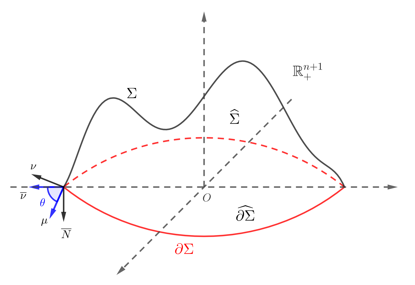
Figure 1. A capillary hypersurface $\Sigma$ with a contact angle $\theta$

The second fundamental form of $\partial\Sigma$ in $\mathbb{R}^{n}$ is given by

$$\widehat{h}(X,Y):=-\langle\nabla^{\mathbb{R}^{n}}_{X}Y,\bar{\nu}\rangle=-\langle D_{X}Y,\bar{\nu}\rangle,\quad X,Y\in T(\partial\Sigma).$$

The second equality holds since $\langle\bar{\nu},\bar{N}\circ x\rangle=0$. The second fundamental form of $\partial\Sigma$ in $\Sigma$ is given by

$$\widetilde{h}(X,Y):=-\langle\nabla_{X}Y,\mu\rangle=-\langle D_{X}Y,\mu\rangle,\quad X,Y\in T(\partial\Sigma).$$

The second equality holds since $\langle\nu,\mu\rangle=0$.

Proposition 2.4.

Let $\Sigma\subset\overline{\mathbb{R}}^{n+1}_{+}$ be a capillary hypersurface. Let $\{e_{\alpha}\}_{\alpha=2}^{n}$ be an orthonormal frame of $\partial\Sigma$. Then along $\partial\Sigma$,

• $\mu$ is a principal direction of $\Sigma$, that is, $h_{\mu\alpha}=h(\mu,e_{\alpha})=0$.

• $h_{\alpha\beta}=\sin\theta\widehat{h}_{\alpha\beta}.$

• $\widetilde{h}_{\alpha\beta}=\cos\theta\widehat{h}_{\alpha\beta}=\cot\theta h_{\alpha\beta}.$

• $h_{\alpha\beta;\mu}=\widetilde{h}_{\beta\gamma}(h_{\mu\mu}\delta_{\alpha\gamma}-h_{\alpha\gamma})$.

Proof.

The first assertion is well-known, see e.g. [47]. (2) and (3) follow from

$$h_{\alpha\beta}=-\langle D_{e_{\alpha}}e_{\beta},\nu\rangle=\langle\widehat{h}_{\alpha\beta}\overline{\nu},\nu\rangle=\sin\theta\widehat{h}_{\alpha\beta},$$

and

$$\widetilde{h}_{\alpha\beta}=-\langle D_{e_{\alpha}}e_{\beta},\mu\rangle=\langle\widehat{h}_{\alpha\beta}\overline{\nu},\mu\rangle=\cos\theta\widehat{h}_{\alpha\beta}.$$

For (4), taking derivative of $h(\mu,e_{\alpha})=0$ with respect to $e_{\beta}$ and using the Codazzi equation and (1), we get

$$0=e_{\beta}(h(\mu,e_{\alpha})) = h_{\alpha\mu;\beta}+h(\nabla_{e_{\beta}}e_{\alpha},\mu)+h(\nabla_{e_{\beta}}\mu,e_{\alpha})$$

$$= h_{\alpha\beta;\mu}+\langle\nabla_{e_{\beta}}e_{\alpha},\mu\rangle h_{\mu\mu}+\langle\nabla_{e_{\beta}}\mu,e_{\gamma}\rangle h_{\alpha\gamma}$$

$$= h_{\alpha\beta;\mu}-\widetilde{h}_{\beta\gamma}(h_{\mu\mu}\delta_{\alpha\gamma}-h_{\alpha\gamma}).$$

∎

The Proposition 2.4 has a direct conseqeunce.

Corollary 2.5.

If $\Sigma$ is a convex capillary hypersurface, then $\partial\Sigma\subset\partial\mathbb{R}^{n+1}$ is also convex, i.e., $\widehat{h}\ \geq 0$, while $\partial\Sigma\subset\Sigma$ is convex $(\widetilde{h}\geq 0)$ if $\theta\in(0,\frac{\pi}{2}]$ and concave $(\widetilde{h}\leq 0)$ if $\theta\in[\frac{\pi}{2},\pi)$.

The following Minkowski type formulas for capillary hypersurfaces play an important role in this paper.

Proposition 2.6.

Let $x:M\to\overline{\mathbb{R}}^{n+1}_{+}$ be an smooth immersion of $\Sigma:=x(M)$ into the half-space, whose boundary intersects $\mathbb{R}^{n}$ with a constant contact angle $\theta\in(0,\pi)$ along $\partial\Sigma$. For $1\leq k\leq n$, it holds

$$\int_{\Sigma}H_{k-1}(1+\cos\theta\langle\nu,e\rangle)dA=\int_{\Sigma}H_{k}\langle x,\nu\rangle dA,$$ (2.13)

where $dA$ is the area element of $\Sigma$ w.r.t. the induced metric $g$.

When $k=1$ or $\theta=\frac{\pi}{2}$, formula (2.13) is known. See e.g. [2, Proof of Theorem 5.1] and [30, Proposition 2.5]. For our purpose, we need the high order Minkowski type formulas for general $\theta$.

Proof.

Denote $x^{T}:=x-\langle x,\nu\rangle\nu$ be the tangential projection of $x$ on $\Sigma$, and

$$P_{e}:=\langle\nu,e\rangle x-\langle x,\nu\rangle e.$$

From a direct computation, we have

$$D_{e_{i}}\langle x,e_{j}\rangle=g_{ij}-\langle x,\nu\rangle h_{ij}$$ (2.14)

and

$$\nabla_{i}(P_{e}^{T})_{j}=\langle\nu,e\rangle g_{ij}+h_{il}\langle e,e_{l}\rangle\langle x,e_{j}\rangle-h_{il}\langle x,e_{l}\rangle\langle e,e_{j}\rangle.$$ (2.15)

Along $\partial\Sigma\subset\partial\mathbb{R}^{n+1}_{+}$, using (2.9) we see

$$\langle P_{e}^{T},\mu\rangle = \langle P_{e},\mu\rangle=\langle\nu,e\rangle\langle x,\mu\rangle-\langle x,\nu\rangle\langle e,\mu\rangle$$

$$= \langle x,-\sin\theta\nu-\cos\theta\mu\rangle,$$

which follows

$$\langle x^{T}+\cos\theta P_{e}^{T},\mu\rangle = \langle x,\mu\rangle-\cos\theta\langle x,\sin\theta\nu+\cos\theta\mu\rangle$$ (2.16)

$$= \sin\theta\langle x,e\rangle=0.$$

Denote $\sigma_{k-1}^{ij}:=\frac{\partial\sigma_{k}}{\partial h^{i}_{j}}$ be the $k$-th Newton transformation. Taking contraction with (2.14), (2.15) and using Proposition 2.1 we obtain

$$\sigma^{ij}_{k-1}\cdot\nabla_{i}\left((x^{T}+\cos\theta P_{e}^{T})_{j}\right) = \sigma_{k-1}^{ij}(g_{ij}-h_{ij}\langle x,\nu\rangle+\cos\theta\langle\nu,e\rangle g_{ij})$$

$$= (n-k+1)\sigma_{k-1}(1+\cos\theta\langle\nu,e\rangle)-k\sigma_{k}\langle x,\nu\rangle$$

$$= \frac{n!}{(k-1)!(n-k)!}\left(H_{k-1}(1+\cos\theta\langle\nu,e\rangle)-H_{k}\langle x,\nu\rangle\right).$$

Using integration by parts, we have

$$\int_{\Sigma}\nabla_{i}\big{(}\sigma^{ij}_{k-1}(x^{T}+\cos\theta P_{e}^{T})_{j}\big{)}dA=\int_{\partial\Sigma}\sigma_{k-1}^{ij}(x^{T}+\cos\theta P_{e}^{T})_{j}\cdot\mu_{i}ds.$$

From (2.16), we know that $(x^{T}+\cos\theta P_{e}^{T})\perp\mu$ along $\partial\Sigma$. Since $\mu$ is a principal direction of $\Sigma$ by Proposition 2.4, we have $\sigma_{k-1}^{ij}(x^{T}+\cos\theta P_{e}^{T})_{j}\cdot\mu_{i}=0$ along $\partial\Sigma$. It is well-known that the Newton tensor is divergence-free, i.e., $\nabla_{i}\sigma_{k-1}^{ij}=0$. Altogether yields the conclusion. ∎

2.5. Variational formulas

The following first variational formula motivates us to define the quermassintegrals for capillary hypersurfaces as (1.8).

Theorem 2.7.

Let $\Sigma_{t}\subset\overline{{\mathbb{R}}}_{+}^{n+1}$ be a family of smooth capillary hypersurfaces supported by $\partial\mathbb{R}^{n+1}_{+}$ with a constant contact angle $\theta\in(0,\pi)$ along $\partial\Sigma_{t}$, given by the embedding $x(\cdot,t):M\to\overline{\mathbb{R}}^{n+1}_{+}$, and satisfying

$$(\partial_{t}x)^{\perp}=f\nu,$$ (2.17)

for a smooth function $f$. Then for $-1\leq k\leq n-1$,

$$\frac{d}{dt}\mathcal{V}_{k+1,\theta}(\widehat{\Sigma_{t}})=\frac{n-k}{n+1}\int_{\Sigma_{t}}fH_{k+1}dA_{t},$$ (2.18)

and

$$\frac{d}{dt}\mathcal{V}_{n+1,\theta}(\widehat{\Sigma_{t}})=0.$$

Before proving Theorem 2.7, we remark that if $\Sigma_{t}\subset\overline{\mathbb{R}}^{n+1}_{+}$ is a family of smooth capillary hypersurfaces evolving by (2.17), then the tangential component $(\partial_{t}x)^{T}$ of $\partial_{t}x$, which we denote by $T\in T\Sigma_{t}$, must satisfy

$$T|_{\partial\Sigma_{t}}=f\cot\theta\mu+\widetilde{T},$$ (2.19)

where $\widetilde{T}\in T(\partial\Sigma_{t})$. In fact, the restriction of $x(\cdot,t)$ on $\partial M$ is contained in $\mathbb{R}^{n}$ and hence,

$$f\nu+T|_{\partial\Sigma_{t}}=\partial_{t}x|_{\partial M}\in T\mathbb{R}^{n}.$$

From (2.9), we know

$$\nu=\frac{1}{\sin\theta}\bar{\nu}-\cot\theta\mu.$$

Since $\bar{\nu}\in T\mathbb{R}^{n}$, it follows $T-f\cot\theta\mu\in T\mathbb{R}^{n}\cap T\Sigma_{t}=T(\partial\Sigma_{t})$, and hence (2.19). Up to a diffeomorphism of $\partial M$, we can assume $\widetilde{T}=0$. For simplicity, in the following, we always assume that

$$T|_{\partial\Sigma_{t}}=f\cot\theta\mu.$$ (2.20)

Hence, from now on, let $\Sigma_{t}$ be a family of smooth, embedding hypersurfaces with $\theta$-capillary boundary in $\overline{\mathbb{R}}^{n+1}_{+}$, given by the embeddings $x(\cdot,t):M\to\overline{\mathbb{R}}^{n+1}_{+}$, which evolves by the general flow

$$\partial_{t}x=f\nu+T,$$ (2.21)

with $T\in T\Sigma_{t}$ satisfying (2.20). We emphasize that the tangential part $T$ plays a key role in the proof of Theorem 2.7 below.

Along flow (2.21), we have the following evolution equations for the induced metric $g_{ij}$, the area element $dA_{t}$, the unit outward normal $\nu$, the second fundamental form $h_{ij}$, the Weingarten matrix $h^{i}_{j}$, the mean curvature $H$, the $k$-th mean curvature $\sigma_{k}$ and $F:=F(h^{j}_{i})$ of the hypersurfaces $\Sigma_{t}$. These evolution equations will be used later.

Proposition 2.8.

Along flow (2.21), it holds that

1. $\partial_{t}g_{ij}=2fh_{ij}+\nabla_{i}T_{j}+\nabla_{j}T_{i}$.

2. $\partial_{t}dA_{t}=\left(fH+{\rm div}(T)\right)dA_{t}.$

3. $\partial_{t}\nu=-\nabla f+h(e_{i},T)e_{i}$.

4. $\partial_{t}h_{ij}=-\nabla^{2}_{ij}f+fh_{ik}h_{j}^{k}+\nabla_{T}h_{ij}+h_{j}^{k}\nabla_{i}T_{k}+h_{i}^{k}\nabla_{j}T_{k}.$

5. $\partial_{t}h^{i}_{j}=-\nabla^{i}\nabla_{j}f-fh_{j}^{k}h^{i}_{k}+\nabla_{T}h^{i}_{j}.$

6. $\partial_{t}H=-\Delta f-|h|^{2}f+\langle\nabla H,T\rangle$.

7. $\partial_{t}\sigma_{k}=-\frac{\partial\sigma_{k}}{\partial h_{i}^{j}}\nabla^{i}\nabla_{j}f-f(\sigma_{1}\sigma_{k}-(k+1)\sigma_{k+1})+\langle\nabla\sigma_{k},T\rangle$.

8. $\partial_{t}F=-F^{j}_{i}\nabla^{i}\nabla_{j}f-fF^{j}_{i}h_{j}^{k}h^{i}_{k}+\langle\nabla F,T\rangle$, where $F^{i}_{j}:=\frac{\partial F}{\partial h^{j}_{i}}$.

The proof of Proposition 2.8 for $T=0$ can be found for example in [27, Chapter 2, Section 2.3] or [21, Appendix B]. A proof for a general $T$ can be found in [59, Proposition 2.11].

Now we complete the proof of Theorem 2.7.

Proof of Theorem 2.7.

Choose an orthonormal frame $\{e_{\alpha}\}_{\alpha=2}^{n}$ of $T{\partial\Sigma}\subset T\mathbb{R}^{n}$ such that $\{e_{1}:=\mu,(e_{\alpha})_{\alpha=2}^{n}\}$ forms an orthonormal frames for $T\Sigma$. First, by taking time derivative to the capillary boundary condition, $\langle\nu,\overline{N}\circ x\rangle=-\cos\theta$ along $\partial\Sigma$, we obtain

$$0 = \langle\partial_{t}\nu,\overline{N}(x(\cdot,t))\rangle+\langle\nu,d\overline{N}(f\nu+T)\rangle$$

$$= \langle-\nabla f+h(e_{i},T)e_{i},\overline{N}\rangle$$

$$= -\sin\theta\nabla_{\mu}f+\sin\theta h(e_{i},T)\langle e_{i},\mu\rangle$$

$$= -\sin\theta\nabla_{\mu}f+\sin\theta h(\mu,\mu)\cot\theta f,$$

where we have used (2.9), Proposition 2.8 and $T|_{\partial M}=f\cot\theta\mu$. As a result,

$$\nabla_{\mu}f=\cot\theta h(\mu,\mu)f\text{ on }\partial\Sigma_{t}.$$ (2.22)

Next, using integration by parts and Proposition 2.8 we have

$$\frac{d}{dt}\left(\int_{\Sigma_{t}}\sigma_{k}dA_{t}\right) = \int_{\Sigma_{t}}\big{[}(\partial_{t}\sigma_{k})dA_{t}+\sigma_{k}\partial_{t}(dA_{t})\big{]}$$ (2.23)

$$= \int_{\Sigma_{t}}\frac{\partial\sigma_{k}}{\partial h_{i}^{j}}\big{(}-f^{i}_{;j}-fh_{ik}h^{kj}+\langle\nabla h^{i}_{j},T\rangle\big{)}dA_{t}+\int_{\Sigma}\sigma_{k}\big{(}f\sigma_{1}+{\rm div}(T)\big{)}dA_{t}$$

$$= -\int_{\partial\Sigma_{t}}\frac{\partial\sigma_{k}}{\partial h^{j}_{i}}f^{i}\mu_{j}+\int_{\partial\Sigma_{t}}\sigma_{k}\langle T,\mu\rangle+\int_{\Sigma_{t}}f\big{(}\sigma_{1}\sigma_{k}-\frac{\partial\sigma_{k}}{\partial h^{j}_{i}}h_{ik}h^{kj}\big{)}dA_{t}$$

$$= \int_{\partial\Sigma_{t}}\big{(}f\sigma_{k}\cot\theta-\frac{\partial\sigma_{k}}{\partial h^{j}_{i}}f^{i}\mu_{j}\big{)}+(k+1)\int_{\Sigma_{t}}f\sigma_{k+1}dA_{t}$$

$$= \int_{\partial\Sigma_{t}}\cot\theta f\sigma_{k}(h|h_{11})+(k+1)\int_{\Sigma_{t}}f\sigma_{k+1}dA_{t},$$

where we have used $T|_{\partial M}=f\cot\theta\mu$, (2.22) and Lemma 2.1 (1), (4).

Moreover flow (3.1) induces a hypersurface flow $\partial\Sigma_{t}\subset\mathbb{R}^{n}$ with normal speed $\frac{f}{\sin\theta}$, that is,

$$\partial_{t}x|_{\partial M}=f\nu+f\cot\theta\mu=\frac{f}{\sin\theta}\overline{\nu}.$$

By (2.2), we have

$$\frac{d}{dt}\mathcal{V}_{k}(\widehat{\partial\Sigma_{t}})=\frac{n-k}{n}\int_{\partial\Sigma_{t}}\frac{f}{\sin\theta}H_{k}^{\partial\Sigma_{t}}(\widehat{h}).$$

From Proposition 2.4 (2), we know

$$h_{\alpha\beta}=\sin\theta\widehat{h}_{\alpha\beta},$$

and hence $\sigma_{k}(h|h_{11})=\sin^{k}\theta\sigma_{k}(\widehat{h})$. Substituting these formulas into (2.23), we obtain

$$\frac{d}{dt}\big{(}\int_{\Sigma_{t}}H_{k}dA_{t}-\sin^{k}\theta\cos\theta\mathcal{V}_{k}(\widehat{\partial\Sigma_{t}})\big{)}=(n-k)\int_{\Sigma_{t}}fH_{k+1}dA_{t}.$$

By the definition of $\mathcal{V}_{k+1,\theta}(\widehat{\Sigma_{t}})$ in (1.8), we get the desired formula (2.18) for $k\geq 0.$

It remains to consider the case $k=-1$. It is easy to check that

$$\mathcal{V}_{0,\theta}(\Sigma_{t})=|\widehat{\Sigma}_{t}|=\frac{1}{n+1}\int_{\Sigma_{t}}\langle x,\nu\rangle dA_{t}.$$

A direct computation gives

$$(n+1)\frac{d}{dt}\mathcal{V}_{0,\theta}(\Sigma_{t}) = \int_{\Sigma_{t}}\left[f-\langle x,\nabla f\rangle+\langle x,\nu\rangle fH+h(T,x^{T})+\langle x,\nu\rangle{\rm div}\,T\right]dA_{t}$$

$$= \int_{\Sigma_{t}}\left((1+{\rm div}(x^{T}))f+\langle x,\nu\rangle fH\right)dA_{t}+\int_{\partial\Sigma_{t}}\left(-\langle x^{T},\mu\rangle f+\langle x,\nu\rangle\langle T,\mu\rangle\right)$$

$$= (n+1)\int_{\Sigma_{t}}fdA_{t},$$

since $-\langle x^{T},\mu\rangle f+\langle x,\nu\rangle\langle T,\mu\rangle=0$ for $x\in\partial\Sigma$, which follows from

$$\langle x,\nu\rangle\langle T,\mu\rangle=f\cot\theta\langle x,\nu\rangle=f\cos\theta\langle x,\bar{\nu}\rangle,$$

$$\langle x^{T},\mu\rangle f=f\cos\theta\langle x,\bar{\nu}\rangle.$$

Now we complete the proof. ∎

3. Locally constrained curvature flow

In this section, we first introduce a new locally constrained curvature flow and show the monotonicity of the quermassintegral along the flow.

Let $M$ be a compact orientable smooth $n$-dimensional manifold. Suppose $x_{0}:M\to\overline{\mathbb{R}}^{n+1}_{+}$ be a smooth initial embedding such that $x_{0}(M)$ is a convex hypersurface in $\overline{\mathbb{R}}^{n+1}_{+}$ and intersects with $\partial{\mathbb{R}}^{n+1}_{+}$ at a constant contact angle $\theta\in(0,{\pi})$. We consider the smooth family of embeddings $x:M\times[0,T)\to\overline{\mathbb{R}}^{n+1}_{+},$ satisfying the following evolution equations

$$\begin{array}[]{rcll}(\partial_{t}x(p,t))^{\perp}&=&f(p,t)\nu&\hbox{ for }(p,t)\in M\times[0,T),\\ \langle\nu(p,t),\overline{N}\circ x(p,t)\rangle&=&\cos(\pi-\theta)&\hbox{ for }(p,t)\in\partial M\times[0,T),\end{array}$$ (3.1)

with $x(M,0)=x_{0}(M)$ and

$$f:=\frac{1+\cos\theta\langle\nu,e\rangle}{F}-\langle x,\nu\rangle,$$ (3.2)

where

$$F:=\frac{H_{l}}{H_{l-1}}.$$ (3.3)

The following nice property of flow (3.1) is essential for us to prove Theorem 1.2 later.

Proposition 3.1.

As long as flow (3.1) exists and $\Sigma_{t}$ is strictly $l$-convex, $\mathcal{V}_{l,\theta}(\widehat{\Sigma_{t}})$ is preserved and $\mathcal{V}_{k,\theta}(\widehat{\Sigma_{t}})$ is non-decreasing for $1\leq k<l\leq n$.

Proof.

From Theorem 2.7, we see

$$\partial_{t}\mathcal{V}_{l,\theta}(\widehat{\Sigma_{t}}) = \frac{n+1-l}{n+1}\int_{\Sigma_{t}}fH_{l}dA_{t}$$

$$= \frac{n+1-l}{n+1}\int_{\Sigma_{t}}\left[\left(1+\cos\theta\langle\nu,e\rangle\right)H_{l-1}-H_{l}\langle x,\nu\rangle\right]dA_{t}$$

$$= 0,$$

where the last equality follows from (2.13). For $1\leq k<l\leq n$, from Theorem 2.7

$$\partial_{t}\mathcal{V}_{k,\theta}(\widehat{\Sigma_{t}}) = \frac{n+1-k}{n+1}\int_{\Sigma_{t}}fH_{k}dA_{t}$$

$$= \frac{n+1-k}{n+1}\int_{\Sigma_{t}}\left[H_{k}\frac{H_{l-1}}{{H_{l}}}\big{(}1+\cos\theta\langle\nu,e\rangle\big{)}-H_{k}\langle x,\nu\rangle\right]dA_{t}$$

$$\geq \frac{n+1-k}{n+1}\int_{\Sigma_{t}}\left[H_{k-1}\big{(}1+\cos\theta\langle\nu,e\rangle\big{)}-H_{k}\langle x,\nu\rangle\right]dA_{t}$$

$$= 0,$$

where we have used the Newton-MacLaurin inequality (2.1) and the Minkowski formula (2.13) in the last two steps respectively. ∎

4. A priori estimates and convergence

The main result of this section is the following long-time existence and the convergence result of flow (3.1) with $l=n$, i.e.,

$$F=\frac{H_{n}}{H_{n-1}}$$ (4.1)

under an angle constraint

$$\theta\in(0,\frac{\pi}{2}].$$

Theorem 4.1.

Assume $x_{0}:M\to\overline{\mathbb{R}}^{n+1}_{+}$ is an embedding of a strictly convex capillary hypersurface in the half-space with the contact angle $\theta\in(0,\frac{\pi}{2}]$. Then there exists $x:M\times[0,+\infty)\to\overline{\mathbb{R}}^{n+1}_{+}$ satisfying flow (3.1) with $F$ given by (4.1) and the initial condition $x(M,0)=x_{0}(M)$. Moreover, $x(\cdot,t)\to x_{\infty}(\cdot)$ in $C^{\infty}$ topology as $t\to+\infty$, and the limit $x_{\infty}:M\to\overline{\mathbb{R}}^{n+1}_{+}$ is a spherical cap.

In order to prove this theorem, we need to obtain a priori estimates, which will be given as follows.

4.1. The short time existence

For the short time existence, one can follow the strategy presented in the paper of Huisken-Polden [36] to give a proof for a general initial capillary hypersurface. Since our initial hypersurface is convex, one can prove the short time existence in the class of star-shaped hypersurfaces. In this class, one can in fact reduce flow (3.1) to a scalar flow. Then the short time existence follows clearly from the standard theory for parabolic equations. Therefore we first consider the reduction.

Assume that a capillary hypersurfaces $\Sigma$ is strictly star-shaped with respect to the origin. One can reparametrize it as a graph over $\overline{\mathbb{S}}^{n}_{+}$. Namely, there exists a positive function $r$ defined on $\overline{\SS}^{n}_{+}$ such that

$$\Sigma=\left\{r(X)X|X\in\overline{\SS}^{n}_{+}\right\},$$

where $X:=(X_{1},\ldots,X_{n})$ is a local coordinate of $\overline{\SS}^{n}_{+}$.

We denote $\nabla^{0}$ be the Levi-Civita connection on $\SS^{n}_{+}$ with respect to the standard round metric $\sigma:=g_{{}_{\SS^{n}_{+}}}$, $\partial_{i}:=\partial_{X_{i}}$, $\sigma_{ij}:=\sigma(\partial_{i},\partial_{j})$, $r_{i}:=\nabla^{0}_{i}r$, and $r_{ij}:=\nabla^{0}_{i}\nabla^{0}_{j}r$. The induced metric $g$ on $\Sigma$ is given by

$$g_{ij}=r^{2}\sigma_{ij}+r_{i}r_{j}=e^{2\varphi}\left(\sigma_{ij}+\varphi_{i}\varphi_{j}\right),$$

where $\varphi(X):=\log r(X)$. Its inverse $g^{-1}$ is given by

$$g^{ij}=\frac{1}{r^{2}}\left(\sigma^{ij}-\frac{r^{i}r^{j}}{r^{2}+|\nabla^{0}r|^{2}}\right)=e^{-2\varphi}\left(\sigma^{ij}-\frac{\varphi^{i}\varphi^{j}}{v^{2}}\right),$$

where $r^{i}:=\sigma^{ij}r_{j}$, $\varphi^{i}:=\sigma^{ij}\varphi_{j}$ and $v:=\sqrt{1+|\nabla^{0}\varphi|^{2}}$. The unit outward normal vector field on $\Sigma$ is given by

$$\nu=\frac{1}{v}\left(\partial_{r}-r^{-2}\nabla^{0}r\right)=\frac{1}{v}\left(\partial_{r}-r^{-1}\nabla^{0}\varphi\right).$$

The second fundamental form $h$ on $\Sigma$ is

$$h_{ij}=\frac{e^{\varphi}}{v}\left(\sigma_{ij}+\varphi_{i}\varphi_{j}-\varphi_{ij}\right),$$

and its Weingarten matrix $h^{i}_{j}$ is

$$h_{j}^{i}=g^{ik}h_{kj}=\frac{1}{e^{\varphi}v}\left[\delta^{i}_{j}-(\sigma^{ik}-\frac{\varphi^{i}\varphi^{k}}{v^{2}})\varphi_{kj}\right].$$

The higher order mean curvature $H_{k}$ can also be expressed by $\varphi$. Moreover,

$$\langle x,\nu\rangle=\langle r\partial_{r},\nu\rangle=\frac{e^{\varphi}}{v}.$$

In order to express the capillary boundary condition in terms of the radial function $\varphi$, we use the polar coordinate in the half-space. For $x:=(x^{\prime},x_{n+1})\in\mathbb{R}^{n}\times[0,+\infty)$ and $X:=(\beta,\xi)\in[0,\frac{\pi}{2}]\times\SS^{n-1}$, we have that

$$x_{n+1}=r\cos\beta,\quad|x^{\prime}|=r\sin\beta.$$

Then

$$e_{n+1}=\partial_{x_{n+1}}=\cos\beta\partial_{r}-\frac{\sin\beta}{r}\partial_{\beta}.$$

In these coordinates the standard Euclidean metric is given by

$$|dx|^{2}=dr^{2}+r^{2}\left(d\beta^{2}+\sin^{2}\beta g_{{}_{\SS^{n-1}}}\right).$$

It follows that

$$\langle\nu,e_{n+1}\rangle=\frac{1}{v}\left(\cos\beta+\sin\beta\nabla_{\partial_{\beta}}^{0}\varphi\right).$$

Along $\partial\SS^{n}_{+}$ it holds

$$\overline{N}\circ x=-e_{n+1}=\frac{1}{r}\partial_{\beta},$$

which yields

$$-\cos\theta=\langle\nu,\overline{N}\circ x\rangle=\langle\frac{1}{v}\left(\partial_{r}-r^{-1}\nabla^{0}\varphi\right),\frac{1}{r}\partial_{\beta}\rangle=-\frac{\nabla^{0}_{\partial_{\beta}}\varphi}{v},$$

that is,

$$\nabla^{0}_{\partial_{\beta}}\varphi=\cos\theta\sqrt{1+|\nabla^{0}\varphi|^{2}}.$$ (4.2)

Therefore, in the class of star-shaped hypersurfaces flow (3.1) is reduced to the following scalar parabolic equation with an oblique boundary condition

$$\begin{array}[]{rcll}\partial_{t}\varphi&=&\frac{v}{e^{\varphi}}f,&\text{ in }\SS^{n}_{+}\times[0,T^{*}),\\ \nabla_{\partial_{\beta}}^{0}\varphi&=&\cos\theta\sqrt{1+|\nabla^{0}\varphi|^{2}},&\text{ on }\partial\SS^{n}_{+}\times[0,T^{*}),\\ \varphi(\cdot,0)&=&\varphi_{0}(\cdot),&\text{ on }\SS^{n}_{+},\end{array}$$ (4.6)

where $\varphi_{0}$ is the parameterization radial function of $x_{0}(M)$ over $\overline{\SS}^{n}_{+}$, and

$$f=\frac{H_{n-1}}{H_{n}}\left[1-\frac{\cos\theta}{v}\left(\cos\beta+\sin\beta\nabla^{0}_{\partial_{\beta}}\varphi\right)\right]-\frac{e^{\varphi}}{v}.$$

Since $|\cos\theta|<1$, the oblique boundary condition (4.2) satisfies the non-degeneracy condition in [44], see also [20]. Hence the short time existence follows.

4.2. Barriers

Let $T^{*}$ be the maximal time of smooth existence of a solution to (3.1), more precisely in the class of star-shaped hypersurfaces. It is obvious that $F$ can not be zero and hence $F$ is positive in $M\times[0,T^{*})$. The positivity of $F$ implies that $\Sigma_{t}$ is strictly convex up to $T^{*}$.

The convexity of $\Sigma_{0}$ implies that there exists some $0<r_{1}<r_{2}<\infty$, such that

$$\Sigma_{0}\subset\widehat{C_{r_{2},\theta}}\setminus\widehat{C_{r_{1},\theta}}.$$

The family of $C_{r,\theta}$ forms natural barriers of (3.1). Therefore, we can show that the solution to (4.6) is uniformly bounded from above and below.

Proposition 4.2.

For any $t\in[0,T^{*})$, $\Sigma_{t}$ satisfies

$$\Sigma_{t}\subset\widehat{C_{r_{2},\theta}}\setminus\widehat{C_{r_{1},\theta}}.$$

Proof.

Recall that $C_{r,\theta}$ satisfies (2.4). Thus for each $r>0$, it is a static solution to flow (3.1). The assertion follows from the avoidance principle for strictly parabolic equation with a capillary boundary condition (see [5, Section 2.6] or [54, Proposition 4.2]). ∎

4.3. Evolution equations of $F$ and $H$

We first introduce a parabolic operator for (3.1)

$$\mathcal{L}:=\partial_{t}-\frac{1+\cos\theta\langle\nu,e\rangle}{F^{2}}F^{ij}\nabla_{ij}^{2}-\langle T+x-\frac{\cos\theta}{F}e,\nabla\rangle.$$

Set $\mathcal{F}:=\sum_{i=1}^{n}F^{i}_{i}$. Using Proposition 2.1 we have

$$\mathcal{F}-\frac{F^{ij}h_{ij}}{F} = \mathcal{F}-1\geq 0,$$ (4.7)

$$\frac{F^{ij}h_{i}^{k}h_{kj}}{F^{2}} = 1.$$ (4.8)

Proposition 4.3.

Along flow (3.1), we have

$$\mathcal{L}F=2\cos\theta F^{-2}F^{ij}F_{;j}h_{ik}\langle e_{k},e\rangle-2(1+\cos\theta\langle\nu,e\rangle)F^{-3}F^{ij}F_{;i}F_{;j}+F\left(1-\frac{F^{ij}(h^{2})_{ij}}{F^{2}}\right),$$

and

$$\nabla_{\mu}F=0,\quad\text{ on }\partial\Sigma_{t}.$$ (4.9)

Proof.

Using the Codazzi formula, we have

$$F^{ij}\langle x,\nu\rangle_{;ij} =F^{ij}\left(h_{ij}+h_{ij;k}\langle x,e_{k}\rangle-(h^{2})_{ij}\langle x,\nu\rangle\right)$$

$$=F+F_{;k}\langle x,e_{k}\rangle-F^{ij}(h^{2})_{ij}\langle x,\nu\rangle,$$

and

$$F^{ij}\langle\nu,e\rangle_{;ij} = F^{ij}\big{(}h_{ik;j}\langle e_{k},e\rangle-(h^{2})_{ij}\langle\nu,e\rangle\big{)}$$

$$= F_{;k}\langle e_{k},e\rangle-F^{ij}(h^{2})_{ij}\langle\nu,e\rangle.$$

Combining with Proposition 2.8, we obtain

$$\partial_{t}F = -F^{ij}f_{;ij}-fF^{ij}(h^{2})_{ij}+\langle\nabla F,T\rangle$$

$$= -F^{ij}\big{(}\frac{1+\cos\theta\langle\nu,e\rangle}{F}-\langle x,\nu\rangle\big{)}_{;ij}-fF^{ij}(h^{2})_{ij}+\langle\nabla F,T\rangle$$

$$= -\cos\theta F^{ij}F^{-1}\langle\nu,e\rangle_{;ij}+2\cos\theta F^{-2}F^{ij}F_{;j}\langle\nu,e\rangle_{;i}-2(1+\cos\theta\langle\nu,e\rangle)F^{-3}F^{ij}F_{;i}F_{;j}$$

$$+F^{-2}F^{ij}F_{;ij}(1+\cos\theta\langle\nu,e\rangle)+\big{(}F+F_{;k}\langle x,e_{k}\rangle-F^{ij}(h^{2})_{ij}\langle x,\nu\rangle\big{)}$$

$$-(1+\cos\theta\langle\nu,e\rangle)F^{-1}F^{ij}(h^{2})_{ij}+\langle x,\nu\rangle F^{ij}(h^{2})_{ij}+\langle\nabla F,T\rangle.$$

Hence it follows

$$\mathcal{L}F = \partial_{t}F-(1+\cos\theta\langle\nu,e\rangle)F^{-2}F^{ij}F_{;ij}-\langle T+x-\cos\theta F^{-1}e,\nabla F\rangle$$

$$= \cos\theta F^{ij}(h^{2})_{ij}F^{-1}\langle\nu,e\rangle+2\cos\theta F^{-2}F^{ij}F_{;j}h_{ik}\langle e_{k},e\rangle-2(1+\cos\theta\langle\nu,e\rangle)F^{-3}F^{ij}F_{;i}F_{;j}$$

$$+\big{(}F-F^{ij}(h^{2})_{ij}\langle x,\nu\rangle\big{)}-(1+\cos\theta\langle\nu,e\rangle)F^{-1}F^{ij}(h^{2})_{ij}+\langle x,\nu\rangle F^{ij}(h^{2})_{ij}$$

$$= 2\cos\theta F^{-2}F^{ij}F_{;j}h_{ik}\langle e_{k},e\rangle-2(1+\cos\theta\langle\nu,e\rangle)F^{-3}F^{ij}F_{;i}F_{;j}$$

$$+F-F^{-1}F^{ij}(h^{2})_{ij}.$$

Along $\partial\Sigma_{t},$ from (2.22) we know

$$\nabla_{\mu}f=\cot\theta h(\mu,\mu)f,$$

By (2.9) or (2.12) and Proposition 2.4 (1), we have on $\partial\Sigma_{t}$

$$\nabla_{\mu}\langle x,\nu\rangle=\langle x,h(\mu,\mu)\mu\rangle=\cos\theta h(\mu,\mu)\langle x,\overline{\nu}\rangle=\cot\theta h(\mu,\mu)\langle x,\nu\rangle,$$

and hence

$$\nabla_{\mu}(f+\langle x,\nu\rangle)=\cot\theta h(\mu,\mu)(f+\langle x,\nu\rangle).$$

Using (2.9) and Proposition 2.4 (1) again, we have ($e=\overline{N}$)

$$\nabla_{\mu}\langle\nu,e\rangle=h(\mu,\mu)\langle\mu,e\rangle=-\tan\theta h(\mu,\mu)\langle\nu,e\rangle$$

and

$$\nabla_{\mu}\big{(}1+\cos\theta\langle\nu,e\rangle\big{)}=-\sin\theta h(\mu,\mu)\langle\nu,e\rangle,$$

where we used $\langle e,\overline{\nu}\rangle=0$ and $\langle e,x\rangle=0$ on $\partial\Sigma_{t}$. One can easily check that the left hand side of the previous formula equals to $\cot\theta h(\mu,\mu)(1+\cos\theta\langle\nu,e\rangle)$, on $\partial\Sigma$. Hence it follows that

$$\nabla_{\mu}F = \nabla_{\mu}\big{(}\frac{1+\cos\theta\langle\nu,e\rangle}{f+\langle x,\nu\rangle}\big{)}=0.$$

∎

We remark that (4.9) plays an important role in applying the maximum principle later. This property holds for curvature flow of free boundary hypersurfaces and capillary hypersurfaces, see also [48, 59].

Proposition 4.4.

Along flow (3.1), we have

$$\mathcal{L}H = (1+\cos\theta\langle\nu,e\rangle)F^{-2}F^{kl,st}h_{kl;i}h_{st;i}+(2+\cos\theta\langle\nu,e\rangle)H$$

$$+\Big{[}2\cos\theta F^{-2}F_{;i}\langle\nu,e\rangle_{;i}-2\left(1+\cos\theta\langle\nu,e\rangle\right)F^{-3}|\nabla F|^{2}$$

$$-(2+\cos\theta\langle\nu,e\rangle)F^{-1}|h|^{2}\Big{]},$$

and, while $\Sigma$ is convex,

$$\nabla_{\mu}H\leq 0,\quad\text{ on }\partial\Sigma_{t}.$$ (4.11)

Proof.

First, note that

$$\Delta\langle\nu,e\rangle=H_{;k}\langle e_{k},e\rangle-|h|^{2}\langle\nu,e\rangle,$$

$$\Delta\langle x,\nu\rangle=H+H_{;k}\langle x,e_{k}\rangle-|h|^{2}\langle x,\nu\rangle.$$

Applying Proposition 2.8, we obtain

$$\partial_{t}H = -\Delta f-|h|^{2}f+\langle\nabla H,T\rangle$$

$$= (1+\cos\theta\langle\nu,e\rangle)F^{-2}\Delta F-2(1+\cos\theta\langle\nu,e\rangle)F^{-3}|\nabla F|^{2}$$

$$+2\cos\theta F^{-2}F_{;i}\langle\nu,e\rangle_{;i}-\cos\theta F^{-1}\Delta\langle\nu,e\rangle+\Delta\langle x,\nu\rangle$$

$$-(1+\cos\theta\langle\nu,e\rangle)F^{-1}|h|^{2}+\langle x,\nu\rangle|h|^{2}+\langle\nabla H,T\rangle$$

$$= (1+\cos\theta\langle\nu,e\rangle)F^{-2}\Delta F-2(1+\cos\theta\langle\nu,e\rangle)F^{-3}|\nabla F|^{2}$$

$$+2\cos\theta F^{-2}F_{;i}\langle\nu,e\rangle_{;i}-F^{-1}|h|^{2}+H$$

$$+\langle x,\nabla H\rangle+\langle\nabla H,T\rangle-\cos\theta F^{-1}\langle e,\nabla H\rangle.$$

The Ricci equation and the Codazzi equation yield

$$h_{kl;ii} = h_{ki;li}=h_{ki;il}+R^{p}_{ili}h_{pk}+R^{p}_{kli}h_{pi}$$

$$= h_{ii;kl}+(h_{pl}H-h_{pi}h_{li})h_{pk}+(h_{pl}h_{ki}-h_{pi}h_{kl})h_{pi}$$

$$= H_{;kl}+h_{pk}h_{pl}H-|h|^{2}h_{kl},$$

which implies

$$\Delta F = \frac{\partial^{2}F}{\partial h_{kl}\partial h_{st}}h_{kl;i}h_{st;i}+F^{kl}h_{kl;ii}$$

$$= F^{kl,st}h_{kl;i}h_{st;i}+F^{kl}H_{;kl}+F^{kl}(h^{2})_{kl}H-F|h|^{2}.$$

Hence we have

$$\mathcal{L}H = \partial_{t}H-F^{-2}(1+\cos\theta\langle\nu,e\rangle)F^{ij}H_{;ij}-\langle T+x-\cos\theta F^{-1}e,\nabla H\rangle$$

$$= (1+\cos\theta\langle\nu,e\rangle)F^{-2}\big{[}F^{kl,st}h_{kl;i}h_{st;i}+F^{kl}(h^{2})_{kl}H-F|h|^{2}\big{]}$$

$$-2(1+\cos\theta\langle\nu,e\rangle)F^{-3}|\nabla F|^{2}+2\cos\theta F^{-2}F_{;i}\langle\nu,e\rangle_{;i}-F^{-1}|h|^{2}+H$$

$$= (1+\cos\theta\langle\nu,e\rangle)F^{-2}F^{kl,st}h_{kl;i}h_{st;i}+(2+\cos\theta\langle\nu,e\rangle)H$$

$$+\Big{[}2\cos\theta F^{-2}F_{;i}\langle\nu,e\rangle_{;i}-2(1+\cos\theta\langle\nu,a\rangle)F^{-3}|\nabla F|^{2}$$

$$-(2+\cos\theta\langle\nu,e\rangle)F^{-1}|h|^{2}\Big{]}.$$

Along $\partial\Sigma_{t}$, choosing an orthonormal frame $\{e_{\alpha}\}_{\alpha=2}^{n}$ of $T{\partial\Sigma_{t}}$ such that $\{e_{1}:=\mu,(e_{\alpha})_{\alpha=2}^{n}\}$ forms an orthonormal frames for $T\Sigma_{t}$. From Proposition 2.4, we have

$$h_{\alpha\beta;\mu}=\cos\theta\widehat{h}_{\beta\gamma}(h_{11}\delta_{\alpha\gamma}-h_{\alpha\gamma}),$$

for all $2\leq\alpha\leq n$. Equation (4.9) implies

$$0=\nabla_{\mu}F=F^{11}h_{11;1}+\sum\limits_{\alpha=2}^{n}F^{\alpha\alpha}h_{\alpha\alpha;1},$$

which in turn implies

$$\nabla_{\mu}H = h_{11;1}+\sum_{\alpha=2}^{n}h_{\alpha\alpha;1}$$

$$= -\sum_{\alpha=2}^{n}\frac{F^{\alpha\alpha}}{F^{11}}h_{\alpha\alpha;1}+\sum_{\alpha=2}^{n}h_{\alpha\alpha;1}=\sum_{\alpha=2}^{n}\frac{1}{F^{11}}\big{(}F^{11}-F^{\alpha\alpha}\big{)}h_{\alpha\alpha;1}$$

$$= \sum_{\alpha=2}^{n}\frac{1}{F^{11}}\big{(}F^{11}-F^{\alpha\alpha}\big{)}(h_{11}-h_{\alpha\alpha})\widetilde{h}_{\alpha\alpha}$$

$$\leq 0,$$

where the last inequality follows from the concavity of $F$, and the convexity of $\partial\Sigma\subset\Sigma$, see Corollary 2.5. Hence (4.11) is proved. ∎

Remark 4.5.

(4.11) is the only place where we have used $\theta\in(0,\frac{\pi}{2}]$.

4.4. Curvature estimates

First, we have the uniform bound of $F$, which follows directly from Proposition 4.3 and the maximum principle.

Proposition 4.6.

Along flow (3.1), it holds

$$\min_{M}F(\cdot,0)\leq F(p,t)\leq\max_{M}F(\cdot,0),\quad\forall(p,t)\in M\times[0,T^{*}).$$

In particular, from the uniform lower bound of $F:=\frac{H_{n}}{H_{n-1}}$, we get a uniform curvature positive lower bound.

Corollary 4.7.

$\Sigma_{t},t\in[0,T^{*})$ is uniformly convex, that is, there exists $c>0$ depending only on $\Sigma_{0}$, such that the principal curvatures of $\Sigma_{t}$,

$$\min_{i}\kappa_{i}(p,t)\geq c,$$

for all $(p,t)\in M\times[0,T^{*})$.

Next we obtain the uniform bound of the mean curvature.

Proposition 4.8.

There exists $C>0$ depending only on $\Sigma_{0}$, such that

$$H(p,t)\leq C,\quad\forall(p,t)\in M\times[0,T^{*}).$$

Proof.

From (4.11), we know that $\nabla_{\mu}H\leq 0$ on $\partial\Sigma_{t}$. Thus $H$ attains its maximum value at some interior point, say $p_{0}\in\text{int}(M)$. We now compute at $p_{0}$.

From the concavity of $F=\frac{n\sigma_{n}}{\sigma_{n-1}}$ in Proposition 2.2, we know

$$\left(1+\cos\theta\langle\nu,e\rangle\right)F^{-2}F^{kl,st}h_{kl;i}h_{st;i}\leq 0.$$

Using Proposition 4.4, we have

$$\mathcal{L}H \leq (2+\cos\theta\langle\nu,e\rangle)H$$

$$+\Big{[}2\cos\theta F^{-2}F_{;i}\langle\nu,e\rangle_{;i}-2\left(1+\cos\theta\langle\nu,e\rangle\right)F^{-3}|\nabla F|^{2}-(2+\cos\theta\langle\nu,e\rangle)F^{-1}|h|^{2}\Big{]}$$

$$:= \text{K}_{1}+\text{K}_{2},$$

The term $|\text{K}_{1}|$ is bounded by $3H$. For the term $\text{K}_{2}$, we note that

$$F\text{K}_{2} := 2\cos\theta F^{-1}F_{;i}\langle\nu,e\rangle_{;i}-2(1+\cos\theta\langle\nu,e\rangle)F^{-2}|\nabla F|^{2}-(2+\cos\theta\langle\nu,e\rangle)|h|^{2}$$

$$= 2\cos\theta F^{-1}F_{;i}h_{ii}\langle e,e_{i}\rangle-2(1+\cos\theta\langle\nu,e\rangle)F^{-2}|\nabla F|^{2}-(2+\cos\theta\langle\nu,e\rangle)|h|^{2}$$

$$:= -\sum_{i=1}^{n}\big{(}\text{S}_{1}F_{;i}^{2}+\text{S}_{2,i}F_{;i}h_{ii}+\text{S}_{3}h_{ii}^{2}\big{)}=-\text{S}_{1}\sum_{i=1}^{n}{\left(F_{;i}-\frac{\text{S}_{2,i}}{2\text{S}_{1}}h_{ii}\right)^{2}}+\sum_{i=1}^{n}\left(\frac{\text{S}_{2,i}^{2}}{4\text{S}_{1}}-\text{S}_{3}\right)h_{ii}^{2},$$

where we have used the notations

$$\text{S}_{1}:=2(1+\cos\theta\langle\nu,e\rangle)F^{-2},\quad{\text{S}_{2,i}:=-2\cos\theta F^{-1}\langle e,e_{i}\rangle},\quad\text{S}_{3}:=2+\cos\theta\langle\nu,e\rangle.$$

One can check

$$\text{S}_{2,i}^{2}-4\text{S}_{1}\text{S}_{3} := 4\cos^{2}\theta F^{-2}\langle e,e_{i}\rangle^{2}-8(1+\cos\theta\langle\nu,e\rangle)F^{-2}(2+\cos\theta\langle\nu,e\rangle)$$

$$\leq 4F^{-2}\Big{[}\cos^{2}\theta|e^{T}|^{2}-2(1+\cos\theta\langle\nu,e\rangle)(2+\cos\theta\langle\nu,e\rangle)\Big{]}$$

$$= 4F^{-2}\Big{[}-3(1+\cos\theta\langle\nu,e\rangle)^{2}-1+\cos^{2}\theta\Big{]}$$

$$\leq -c_{0}$$

for some positive constant $c_{0}$. Combining with Proposition 4.6, it implies

$$\text{K}_{2}\leq-\frac{c_{0}}{4F\text{S}_{1}}|h|^{2}=-\frac{c_{0}F}{8(1+\cos\theta\langle\nu,e\rangle)}|h|^{2}\leq-C|h|^{2},$$

for some positive constant $C>0$. Therefore,

$$0\leq\mathcal{L}H(p_{0})\leq\text{K}_{1}+\text{K}_{2}\leq 3H-C|h|^{2},$$

which yields that $H$ is uniformly bounded from above. ∎

Proposition 4.8 and Corollary 4.7 imply directly that

Corollary 4.9.

$\Sigma_{t},t\in[0,T^{*})$, has a uniform curvature bound, namely, there exists $C>0$ depending only on $\Sigma_{0}$, such that the principal curvatures of $\Sigma_{t}$,

$$\max_{i}\kappa_{i}(p,t)\leq C,$$

for all $(p,t)\in M\times[0,T^{*})$.

4.5. Convergence of the flow

First we show that the convexity implies that the star-shaped is preserved in the following sense.

Proposition 4.10.

There exists $c_{0}>0$ depending only on $\Sigma_{0}$, such that

$$\langle x,\nu\rangle(p,t)\geq c_{0}.$$ (4.12)

for all $(p,t)\in M\times[0,T^{*})$.

Proof.

For any $T^{\prime}<T^{*}$, assume $\min\limits_{M\times[0,T^{\prime}]}\langle x,\nu\rangle(p,t)=\langle x,\nu\rangle(p_{0},t_{0})$. Then, either $p_{0}\in\partial M$ or $p_{0}\in M\setminus\partial M$.

If $p_{0}\in M\setminus\partial M$, let $\{e_{i}\}_{i=1}^{n}$ be the orthonormal frame of $\Sigma_{t}$, then at $p_{0}$,

$$0=D_{e_{i}}\langle x,\nu\rangle=h_{ij}\langle x,e_{j}\rangle.$$

Due to the strict convexity $(h_{ij})>0$, we have $\langle x,e_{i}\rangle=0$. It follows

$$\langle x,\nu\rangle(p_{0})=|x|(p_{0})\geq c_{0},$$

for some $c_{0}>0$, which depends only on the initial datum.

If $p_{0}\in\partial M$, by (2.9) we have

$$\langle x,\nu\rangle=\langle x,\sin\theta\overline{\nu}-\cos\theta e\rangle=\sin\theta\langle x,\overline{\nu}\rangle.$$

Hence $\langle x,\overline{\nu}\rangle\big{|}_{\partial M}$ attains its minimum value at $p_{0}$. As above, choosing $\{e_{\alpha}\}_{\alpha=2}^{n}$ be the orthonormal frame of $\partial\Sigma_{t}$ in $\mathbb{R}^{n}$ such that $e_{1}=\overline{\nu}$, we have

$$0=\nabla^{\mathbb{R}^{n}}_{e_{\alpha}}\langle x,\overline{\nu}\rangle=\widehat{h}_{\alpha\beta}\langle x,e_{\beta}\rangle,$$

By Proposition 2.4 (2) and Corollary 4.7, we know $(\widehat{h}_{\alpha\beta})>0$, and hence we have $x\parallel\overline{\nu}$ at $p_{0}$ and

$$\langle x,\overline{\nu}\rangle(p_{0})=|x|(p_{0})\geq c_{0},$$

for some $c_{0}>0$, which depends only on the initial datum. Therefore, we finish the proof of (4.12). ∎

Proposition 4.11.

Flow (3.1) exists for all time with uniform $C^{\infty}$-estimates.

Proof.

From Proposition 4.2, Proposition 4.10, Proposition 4.7 and Corollary 4.9, we see that $\varphi$ is uniformly bounded in $C^{2}(\mathbb{S}^{n}_{+}\times[0,T^{*}))$ and the scalar equation in (4.6) is uniformly parabolic. Since $|\cos\theta|<1$, the boundary value condition in (4.6) satisfies the uniformly oblique property. From the standard parabolic theory (see e.g. [20, Theorem 6.1, Theorem 6.4 and Theorem 6.5], also [52, Theorem 5] and [39, Theorem 14.23]), we conclude the uniform $C^{\infty}$-estimates and the long-time existence of solution to (4.6).

∎

Proposition 4.12.

$x(\cdot,t)$ smoothly converges to a uniquely determined spherical cap around $\cos\theta e$ with capillary boundary, as $t\to\infty$.

Proof.

By Proposition 3.1, we know $\mathcal{V}_{1,\theta}(\widehat{\Sigma_{t}})$ is non-decreasing, due to

$$\partial_{t}\mathcal{V}_{1,\theta}(\widehat{\Sigma_{t}})=\frac{n}{n+1}\int_{\Sigma_{t}}\left(\frac{H_{1}H_{n-1}}{H_{n}}-1\right)\left(1+\cos\theta\langle\nu,e\rangle\right)dA_{t}\geq 0.$$

It follows from the long time existence and uniform $C^{\infty}$-estimates that

$$\int_{0}^{\infty}\partial_{t}\mathcal{V}_{1,\theta}(\widehat{\Sigma_{t}})dt\leq\mathcal{V}_{1,\theta}(\widehat{\Sigma_{\infty}})<+\infty.$$

Then we obtain

$$\int_{\Sigma_{t_{i}}}\left(\frac{H_{1}H_{n-1}}{H_{n}}-1\right)\left(1+\cos\theta\langle\nu,e\rangle\right)dA\to 0,\hbox{ as }t_{i}\to+\infty.$$

Moreover one can show that for any sequence $t_{i}\to\infty$, there exists a convergent subsequence, whose limit satisfying

$$\left(\frac{H_{1}H_{n-1}}{H_{n}}-1\right)\left(1+\cos\theta\langle\nu,e\rangle\right)=0.$$

It is easy to see that the limit is a spherical cap. Next we show that any limit of a convergent subsequence is uniquely determined, which implies the flow smoothly converges to a unique spherical cap. We shall use the argument in [48].

Note that we have proved that $x(\cdot,t)$ subconverges smoothly to a capillary boundary spherical cap $C_{\rho_{\infty},\theta}(e_{\infty})$. Since $\mathcal{V}_{n,\theta}$ is preserved along flow (3.1), the radius $\rho_{\infty}$ is independent of the choice of the subsequence of $t$. We now show in the following that $e_{\infty}=e$. Denote $\rho(\cdot,t)$ be the radius of the unique spherical cap $C_{\rho(\cdot,t),\theta}(e)$ around $e$ with contact angle $\theta$ passing through the point $x(\cdot,t)$. Due to the spherical barrier estimate, i.e. Proposition 4.2, we know

$$\rho_{\max}(t):=\max\rho(\cdot,t)=\rho(\xi_{t},t),$$

is non-increasing with respect to $t$, for some point $\xi_{t}\in M$. Hence the limit $\lim\limits_{t\to+\infty}\rho_{\text{max}}(t)$ exists. Next we claim that

$$\lim_{t\to+\infty}\rho_{\max}(t)=\rho_{\infty}.$$ (4.13)

We prove this claim by contradiction. Suppose (4.13) is not true, then there exists $\varepsilon>0$ such that

$$\rho_{\max}(t)>\rho_{\infty}+{\varepsilon},\hbox{ for }t\hbox{ large enough.}$$ (4.14)

By definition, $\rho(\cdot,t)$ satisfies

$$\rho^{2}\sin^{2}\theta=|x|^{2}-2\rho\cos\theta\langle x,e\rangle.$$ (4.15)

Hence

$$\left(\rho\sin^{2}\theta+\cos\theta\langle x,e\rangle\right)\partial_{t}\rho=\langle\partial_{t}x,x-\rho\cos\theta e\rangle.$$

We evaluate at $(\xi_{t},t)$. Since $\Sigma_{t}$ is tangential to $C_{\rho,\theta}(e)$ at $x(\xi_{t},t)$, we have

$$\nu_{\Sigma_{t}}(\xi_{t},t)=\nu_{\partial C_{r,\theta}(e)}(\xi_{t},t)={\frac{x-\rho\cos\theta e}{\rho}}.$$

Thus we deduce

$${\left(\rho_{\max}\sin^{2}\theta+\cos\theta\langle x,e\rangle\right)\partial_{t}\rho|_{(\xi_{t},t)}}=\rho_{\max}\left(\frac{1+\cos\theta\langle\nu,e\rangle}{F}-\langle x,\nu\rangle\right).$$ (4.16)

We note that there exists some $\delta>0$ such that

$${\rho_{\max}\sin^{2}\theta+\cos\theta\langle x,e\rangle}\geq\delta>0.$$ (4.17)

In fact, this follows directly from (4.15), due to

$${\rho\sin^{2}\theta+\cos\theta\langle x,e\rangle}=\frac{1}{2\rho}(|x|^{2}+\rho^{2}\sin^{2}\theta)\geq\frac{\rho}{2}\sin^{2}\theta>0.$$ (4.18)

Since the spherical caps $C_{\rho_{\max},\theta}(e)$ are the static solutions to (3.1) and $x(\cdot,t)$ is tangential to $C_{\rho_{\max},\theta}(e)$ at $x(\xi_{t},t)$, we see from (2.4)

$$\frac{1+\cos\theta\langle\nu,e\rangle}{\langle x,\nu\rangle}\Big{|}_{x(\xi_{t},t)}=\frac{1+\cos\theta\langle\nu,e\rangle}{\langle x,\nu\rangle}\Big{|}_{C_{\rho_{\max},\theta}(e)}=\frac{1}{\rho_{\max}(t)}.$$ (4.19)

Since $x(\cdot,t)$ subconverges to $C_{\rho_{\infty},\theta}(e_{\infty})$ and $\rho_{\infty}$ is uniquely determined, we have

$$F=\frac{n\sigma_{n}}{\sigma_{n-1}}\to\frac{1}{\rho_{\infty}}\quad\text{uniformly},$$

as $t\to+\infty$. Thus there exists $T_{0}>0$ such that

$$\frac{1}{F}-{\rho_{\infty}}<\frac{\epsilon}{2},$$

and hence

$$\frac{1}{F}-{\rho_{\max}(t)}<-\frac{\epsilon}{2},$$

for all $t>T_{0}$. Taking into account of (4.19), we see

$$\left(\frac{1}{F}-{\frac{\langle x,\nu\rangle}{1+\cos\theta\langle\nu,e\rangle}}\right)\Big{|}_{x(\xi_{t},t)}<-\frac{\epsilon}{2},$$ (4.20)

for all $t>T_{0}$. By adopting Hamilton’s trick, we conclude from (4.16), (4.17) and (4.20) that there exists some $C>0$ such that for almost every $t$,

$$\frac{d}{dt}\rho_{\max}\leq-C\epsilon.$$

This is a contradiction to the fact that $\lim\limits_{t\to+\infty}\frac{d}{dt}\rho_{\max}=0$, and hence claim (4.13) is true. Similarly, we can obtain that

$$\lim_{t\to+\infty}\rho_{\min}(t)=\rho_{\infty}.$$ (4.21)

Hence $\lim\limits_{t\to\infty}\rho(\cdot,t)=\rho_{\infty}$. This implies that any limit of a convergent subsequence is the spherical cap around $e$ with radius $\rho_{\infty}$. We complete the proof of Proposition 4.12.

∎

In view of Proposition 4.11 and Proposition 4.12, Theorem 4.1 are proved.

5. Alexandrov-Fenchel inequalities

In this section, we apply the convergence result of flow (3.1) to prove Theorem 1.2.

Proof of Theorem 1.2.

Remember

$$\mathcal{V}_{k,\theta}(\widehat{C_{r,\theta}})=r^{n+1-k}\mathbf{b}_{\theta},$$ (5.1)

where $\mathbf{b}_{\theta}$ was defined by (2.5).

Assume that $\Sigma$ is strictly convex. We have proved in Section 4 that flow (3.1) converges a spherical cap, which we denote by $C_{r_{\infty},\theta}(e)$. By the monotonicity of $\mathcal{V}_{n,\theta}$ and $\mathcal{V}_{k,\theta}$, Proposition 3.1 we have

$$\mathcal{V}_{n,\theta}(\widehat{\Sigma})=\mathcal{V}_{n,\theta}(\widehat{C_{r_{\infty},\theta}(e)}),\qquad\mathcal{V}_{k,\theta}(\widehat{\Sigma})\leq\mathcal{V}_{k,\theta}(\widehat{C_{r_{\infty},\theta}(e)}),$$

moreover, equality holds iff $\Sigma$ is a spherical cap. It is clear that (5.1) is the same as (1.11).

When $\Sigma$ is convex but not strictly convex, the inequality follows by approximation. The equality characterization can be proved similar to [48, Section 4], by using an argument of [29]. We omit the details here. ∎

For Corollary 1.4, one just notes that when $n=2$,

$$\mathbf{b}_{\theta}=\frac{1}{3}\left(2-3\cos\theta+\cos^{3}\theta\right)\pi.$$

6. Statements and Declarations.

Conflict of interest. On behalf of all authors, the corresponding author states that there is no conflict of interest.

Data sharing not applicable to this article as no datasets were generated or analysed during the current study.

The authors have no relevant financial or non-financial interests to disclose.

Acknowledgment: LW is supported by NSFC (Grant No. 12201003, 12171260). CX is supported by NSFC (Grant No. 11871406, 12271449). We would like to thank the referee for careful reading and valuable suggestions to improve the context of the paper.

References

- [1] Virginia Agostiniani, Mattia Fogagnolo, Lorenzo Mazzieri, Minkowski inequalities via nonlinear potential theory. Arch. Rat. Mech. Anal. 244 (2022), no. 1, 51–85.
- [2] Abdelhamid Ainouz, Rabah Souam, Stable capillary hypersurfaces in a half-space or a slab. Indiana Univ. Math. J. 65 (2016), no. 3, 813–831.
- [3] Aleksandr D. Alexandrov, Zur Theorie der gemischten Volumina von konvexen Körpern, II. Neue Ungleichungen zwischen den gemischten Volumina und ihre Anwendungen, Mat. Sb. (N.S.) 2 (1937) 1205–1238 (in Russian).
- [4] Aleksandr D. Alexandrov, Zur Theorie der gemischten Volumina von konvexen Körpern, III. Die Erweiterung zweeier Lehrsatze Minkowskis über die konvexen Polyeder auf beliebige konvexe Flachen, Mat. Sb. (N.S.) 3 (1938) 27–46 (in Russian).
- [5] Steven J. Altschuler, Langfang Wu, Translating surfaces of the non-parametric mean curvature flow with prescribed contact angle. Calc. Var. Partial Differ. Equ. 2(1), 101–111 (1994).
- [6] Ben Andrews, Yingxiang Hu, Haizhong Li, Harmonic mean curvature flow and geometric inequalities. Adv. Math. 375 (2020), 107393, 28 pp.
- [7] Ben Andrews, Yong Wei, Quermassintegral preserving curvature flow in hyperbolic space. Geom. Funct. Anal. 28 (2018), no. 5, 1183–1208.
- [8] Ben Andrews, Yong Wei, Volume preserving flow by powers of the -th mean curvature. J. Differential Geom. 117 (2021), no. 2, 193–222.
- [9] Jürgen Bokowski, Emanuel Jr. Sperner, Zerlegung konvexer Körper durch minimale Trennflächen. (German) J. Reine Angew. Math. 311(312) (1979), 80–100.
- [10] Simon Brendle, Pengfei Guan, Junfang Li, An inverse curvature type hypersurface flow in space forms, (Private note).
- [11] Yu. D. Burago, V. G. Maz’ya, Potential theory and function theory for irregular regions. Translated from Russian Seminars in Mathematics, V. A. Steklov Mathematical Institute, Leningrad, Vol. 3 Consultants Bureau, New York 1969.
- [12] Herbert Busemann, Minkowski’s and related problems for convex surfaces with boundaries. Michigan Math. J. 6 (1959), 259–266.
- [13] Xavier Cabré, Xavier Ros-Oton, Joaquim Serra, Sharp isoperimetric inequalities via the ABP method. J. Eur. Math. Soc. 18 (2016), no. 12, 2971–2998.
- [14] Sun-Yung Alice Chang, Sun-Yung, Yi Wang, Inequalities for quermassintegrals on -convex domains. Adv. Math. 248 (2013), 335–377.
- [15] Chuanqiang Chen, Pengfei Guan, Junfang Li, Julian Scheuer, A fully nonlinear flow and quermassintegral inequalities. Pure Appl. Math Q. 18, no. 2, p. 437–461, (2022).
- [16] Min Chen, Jun Sun, Alexandrov-Fenchel type inequalities in the sphere. Adv. Math. 397 (2022), Paper No. 108203.
- [17] Jaigyoung Choe, Mohammad Ghomi, Manuel Ritoré, The relative isoperimetric inequality outside convex domains in . Calc. Var. Partial Differential Equations. 29 (2007), no. 4, 421–429.
- [18] Francesco Della Pietra, Carlo Nitsch, Cristina Trombetti, An optimal insulation problem. Math. Ann. 382 (2022), 745–759
- [19] Levi Lopes de Lima, Frederico Giro, An Alexandrov-Fenchel-type inequality in hyperbolic space with an application to a Penrose inequality. Ann. Henri Poincaré 17 (2016), no. 4, 979–1002.
- [20] Guang-chang Dong, Initial and nonlinear oblique boundary value problems for fully nonlinear parabolic equations. J. Partial Differential Equations Ser. A 1 (1988), no. 2, 12–42.
- [21] Klaus Ecker, Regularity theory for mean curvature flow. Progress in Nonlinear Differential Equations and their Applications, 57. Birkhäuser Boston, Inc., Boston, MA, 2004.
- [22] Alessio Figalli, Emanuel Indrei, A sharp stability result for the relative isoperimetric inequality inside convex cones. J. Geom. Anal. 23 (2013), no. 2, 938–969.
- [23] Robert Finn, Equilibrium capillary surfaces. Grundlehren der Mathematischen Wissenschaften, 284. Springer-Verlag, New York, 1986.
- [24] Alexandre Freire, Schwartz Fernando, Mass-capacity inequalities for conformally flat manifolds with boundary. Comm. Partial Differential Equations. 39 (2014), no. 1, 98–119.
- [25] Nicola Fusco, Massimiliano Morini, Total positive curvature and the equality case in the relative isoperimetric inequality outside convex domains. ArXiv:2103.03299.
- [26] Yuxin Ge, Guofang Wang, Jie Wu, Hyperbolic Alexandrov-Fenchel quermassintegral inequalities II. J. Differential Geom. 98 (2014), no. 2, 237–260.
- [27] Claus Gerhardt, Curvature problems. Series in Geometry and Topology, 39. International Press, Somerville, MA, 2006.
- [28] Claus Gerhardt, Flow of nonconvex hypersurfaces into spheres. J. Differential Geom. 32 (1990), no. 1, 299–314.
- [29] Pengfei Guan, Junfang Li, The quermassintegral inequalities for -convex starshaped domains. Adv. Math. 221 (2009), no. 5, 1725–1732.
- [30] Pengfei Guan, Junfang Li, A mean curvature type flow in space forms. Int. Math. Res. Not. 2015, no. 13, 4716–4740.
- [31] Pengfei Guan, Junfang Li, A fully-nonlinear flow and quermassintegral inequalities (in Chinese). Sci. Sin. Math. 48 (2018), no. 1, 147–156.
- [32] Pengfei Guan, Junfang Li, Isoperimetric type inequalities and hypersurface flows J. Math. Study, 54 (2021), no. 1, 56–80.
- [33] Yingxiang Hu, Haizhong Li, Geometric inequalities for static convex domains in hyperbolic space. Trans. Amer. Math. Soc. 375 (2022), 5587–5615
- [34] Yingxiang Hu, Haizhong Li, Yong Wei, Locally constrained curvature flows and geometric inequalities in hyperbolic space. Math. Ann. 382 (2022), no. 3-4, 1425–1474.
- [35] Gerhard Huisken, An isoperimetric concept for the mass in general relativity, 2009. https://www.ias.edu/video/marston-morse-isoperimetric-concept-mass-general-relativity
- [36] Gerhard Huisken, Alexander Polden, Geometric evolution equations for hypersurfaces. Calculus of variations and geometric evolution problems, 45–84, Lecture Notes in Math., 1713, Fond. CIME/CIME Found. Subser., Springer, Berlin, 1999.
- [37] Ben Lambert, Julian Scheuer, A geometric inequality for convex free boundary hypersurfaces in the unit ball. Proc. Amer. Math. Soc. 145 (2017), no. 9, 4009–4020.
- [38] Haizhong Li, Yong Wei, Changwei Xiong, A geometric inequality on hypersurface in hyperbolic space. Adv. Math. 253 (2014), 152–162.
- [39] Gary M. Lieberman, Second order parabolic differential equations. World Scientific Publishing Co., Inc., River Edge, NJ, 1996.
- [40] Lei Liu, Guofang Wang, Liangjun Weng, The relative isoperimetric inequality for minimal submanifolds in the Euclidean space. ArXiv:2002.00914.
- [41] Francesco Maggi, Sets of finite perimeter and geometric variational problems. An introduction to geometric measure theory. Cambridge Studies in Advanced Mathematics, 135. Cambridge University Press, Cambridge, 2012.
- [42] Matthias Makowski, Julian Scheuer, Rigidity results, inverse curvature flows and Alexandrov-Fenchel type inequalities in the sphere. Asian J. Math. 20 (2016), no. 5, 869–892.
- [43] James A. McCoy, Mixed volume preserving curvature flows. Calc. Var. Partial Differential Equations. 24 (2005), no. 2, 131–154.
- [44] A. I. Nazarov, Nina N. Ural’tseva, A problem with an oblique derivative for a quasilinear parabolic equation. (Russian) Zap. Nauchn. Sem. S.-Peterburg. Otdel. Mat. Inst. Steklov. (POMI) 200 (1992), Kraev. Zadachi Mat. Fiz. Smezh. Voprosy Teor. Funkt. 24, 118–131, 189; translation in J. Math. Sci. 77 (1995), no. 3, 3212–3220
- [45] Guohuan Qiu, A family of higher-order isoperimetric inequalities. Commun. Contemp. Math. 17 (2015), no. 3, 1450015, 20 pp.
- [46] Robert C. Reilly, Variational properties of functions of the mean curvatures for hypersurfaces in space forms. J. Differential Geom. 8 (1973), 465–477.
- [47] Antonio Ros, Rabah Souam, On stability of capillary surfaces in a ball. Pacific J. Math. 178 (1997), no. 2, 345–361.
- [48] Julian Scheuer, Guofang Wang, Chao Xia, Alexandrov-Fenchel inequalities for convex hypersurfaces with free boundary in a ball. J. Differential Geom. 120 (2022) no. 2, 345–373.
- [49] Julian Scheuer, Chao Xia, Locally constrained inverse curvature flows. Trans. Amer. Math. Soc. 372 (2019) no. 10, 6771–6803.
- [50] Rolf Schneider, Convex bodies: the Brunn-Minkowski theory. Second expanded edition. Encyclopedia of Mathematics and its Applications, 151. Cambridge University Press, Cambridge, 2014.
- [51] Joel Spruck, Geometric aspects of the theory of fully nonlinear elliptic equations. Global theory of minimal surfaces, 283–309, Clay Math. Proc., 2, Amer. Math. Soc., Providence, RI, 2005.
- [52] Nina N. Ural’tseva, A nonlinear problem with an oblique derivative for parabolic equations. Zap. Nauchn. Sem. Leningrad. Otdel. Mat. Inst. Steklov. (LOMI) 188 (1991).
- [53] John I. E. Urbas, On the expansion of starshaped hypersurfaces by symmetric functions of their principal curvatures. Math. Z. 205 (1990), no. 3, 355–372.
- [54] Guofang Wang, Liangjun Weng, A mean curvature type flow with capillary boundary in a unit ball. Calc. Var. PDEs. 59 (2020), no. 5, Paper No. 149, 26 pp.
- [55] Guofang Wang, Chao Xia, Isoperimetric type problems and Alexandrov-Fenchel type inequalities in the hyperbolic space. Adv. Math. 259 (2014), 532–556.
- [56] Guofang Wang, Chao Xia, Uniqueness of stable capillary hypersurfaces in a ball. Math. Ann. 374 (2019), no. 3-4, 1845–1882.
- [57] Yong Wei, Changwei Xiong, Inequalities of Alexandrov-Fenchel type for convex hypersurfaces in hyperbolic space and in the sphere. Pacific J. Math. 277 (2015), no. 1, 219–239.
- [58] Yong Wei, Changwei Xiong, A volume-preserving anisotropic mean curvature type flow. Indiana Univ. Math. J. 70 (2021), no. 3, 881–905.
- [59] Liangjun Weng, Chao Xia, The Alexandrov-Fenchel inequalities for convex hypersurfaces with capillary boundary in a ball. Trans. Amer. Math. Soc. 375 (2022), 8851–8883.
- [60] Chao Xia, Inverse anisotropic mean curvature flow and a Minkowski type inequality. Adv. Math. 315 (2017), 102–129.