Reflected Entropy in Boundary/Interface Conformal Field Theory

Abstract

Boundary conformal field theory (BCFT) and interface conformal field theory (ICFT) attract attention in the context of the information paradox problem. On this background, we develop the idea of the reflected entropy in BCFT/ICFT. We first introduce the left-right reflected entropy (LRRE) in BCFT and show that its holographic dual is given by the area of the entanglement wedge cross section (EWCS) through AdS/BCFT. We also present how to evaluate the reflected entropy in ICFT. By using this technique, we can show the universal behavior of the reflected entropy in some special classes.

I Introduction

The entanglement entropy (EE) plays a significant role in quantum information, condensed matter, and quantum gravity Ryu and Takayanagi (2006). This quantity captures the bipartite entanglement between a subsystem $A$ and its complement $\bar{A}$. The EE is defined by the von-Neumann entropy for the reduced density matrix $\rho_{A}\equiv{\text{tr}}_{\bar{A}}\rho$ as $S(A)=-{\text{tr}}\rho_{A}\log\rho_{A}$.

One interesting direction to develop this idea is finding a tripartite entanglement measure. Recently, as one of them, the reflected entropy is introduced by Dutta and Faulkner (2021). This quantity is applied to various (1+1)-$d$ setups Dutta and Faulkner (2021); Kudler-Flam et al. (2021, 2020); Kusuki and Tamaoka (2021, 2020); Bueno and Casini (2020a); Zou and Vidal (2022), (2+1)-$d$ setups Liu et al. (2022); Siva et al. (2021); Berthiere et al. (2021), and arbitrary dimensional setups Bueno and Casini (2020b); Camargo et al. (2021). One of the significant features of the reflected entropy is that this quantity has a nice bulk dual, the minimal area of the cross section in the entanglement wedge Dutta and Faulkner (2021). It means that like the EE, one can probe the entanglement structure of quantum gravity by a simple calculation of the area. Another feature is that mostly bipartite entanglement patterns imply that the difference between the reflected entropy and the mutual information is close to zero, $S_{R}-I\simeq 0$ Akers and Rath (2020); Zou et al. (2021) . Inspired by this sensitivity to tripartite entanglement, the difference $S_{R}-I$ is studied in Bueno and Casini (2020a, b); Camargo et al. (2021); Hayden et al. (2021), called the Markov gap.

In this article, we develop the idea of the reflected entropy in boundary CFT (BCFT) and interface CFT (ICFT). BCFT is introduced in Cardy (2004) and developed in many works. In this article, we particularly focus on the left-right entanglement, which is mainly explored in BCFT Pando Zayas and Quiroz (2015); Das and Datta (2015); Affleck et al. (2009). Interface CFT (ICFT) is a class of CFTs where two (possibly different) CFTs are connected along an interface Oshikawa and Affleck (1996, 1997); Bachas et al. (2002). The entanglement entropy in ICFT is studied in various (1+1)-$d$ CFT setups Sakai and Satoh (2008); Brehm and Brunner (2015); Brehm et al. (2016); Wen et al. (2018); Gutperle and Miller (2016a). If one considers the reflected entropy in BCFT/ICFT, one may have several questions, for example, can we directly extract the entanglement wedge cross section between the subsystem and the island (see FIG.5)? how can we evaluate the reflected entropy in ICFTs? We answer these questions. Regarding the first question, we will introduce a new quantity “left-right reflected entropy (LRRE)” and show its holographic dual. In regards to the second question, we will introduce a new technique to evaluate reflected entropy in ICFT/BCFT. This has a wide range of applications. For example, the analysis in Liu et al. (2022) is based on numerical calculation because of a technical reason. We can now overcome this problem by the method developed in this article Liu et al. .

There is another motivation to investigate the reflected entropy in BCFT/ICFT. Recent progress on the information paradox problem is provided in a class of toy models where the black hole and a non-gravitational bath CFT are glued along the (asymptotic) boundary, which is called the island model Penington (2020); Almheiri et al. (2019); Almheiri et al. (2020a). This model is related to BCFT/ICFT through the AdS/BCFT and the braneworld holography Almheiri et al. (2020b); Sully et al. (2021); Akal et al. (2020); Bousso and Wildenhain (2020); Miao (2021); Akal et al. (2021a); Geng and Karch (2020); Geng et al. (2021a); Chu et al. (2021); Akal et al. (2021b); Ageev (2021); Geng et al. (2021b); Kusuki (2022a); Suzuki and Takayanagi (2022); Numasawa and Tsiares (2022); Izumi et al. (2022); Kusuki (2022b).

There are several works about the reflected entropy in the island model Akers et al. (2022); Chandrasekaran et al. (2020); Hayden et al. (2021); Li et al. (2020); Ghodrati (2021). In this context, our new measure in BCFT and new technique in ICFT have the potential to provide a new understanding of the island model.

II Left-Right Mutual Information

The left-right entanglement entropy (LREE) is defined by a reduced density matrix obtained by tracing over the right moving sector Pando Zayas and Quiroz (2015); Das and Datta (2015); Affleck et al. (2009),

$$S^{(l/r)}\equiv-{\text{tr}}\rho^{(L)}\log\rho^{(L)},$$ (1)

where $\rho^{(L)}\equiv{\text{tr}}_{R}\rho$. One can generalize this quantity by considering a reduced density matrix obtained by tracing over the right moving sector and a part of the left moving sector,

$$S^{(L)}(A)\equiv-{\text{tr}}\rho^{(L)}_{A}\log\rho^{(L)}_{A},$$ (2)

where $\rho^{(L)}_{A}\equiv{\text{tr}}_{\bar{A}\cup R}\rho$ . This quantity can be calculated by the replica trick in the same way as in Pando Zayas and Quiroz (2015); Das and Datta (2015); Affleck et al. (2009). One can also calculate it by a correlation function with chiral twist operators . With this quantity, one can introduce an interesting quantum information quantity, which we call the left-right mutual information (LRMI),

$$I^{(l/r)}(A)\equiv S^{(L)}(A)+S^{(R)}(A)-S(A).$$ (3)

The physical interpretation is in the following. Let us consider a local excitation that creates a pair of left and right movers. The LRMI increases if both of them are included in the subsystem $A$. That is, the LRMI counts the number of such pairs (see FIG. 1).

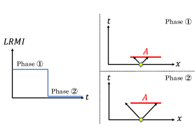
Figure 1: To give an interpretation of the LRMI, it would be nice to consider the time dependence of the LRMI after a local quench in an integrable system. In the phase $\scriptsize1⃝$, both the left and right mover are in the subsystem $A$. This entanglement pair increases the LRMI. In the phase $\scriptsize2⃝$, there is no such a pair in the subsystem $A$. Consequently, the LRMI vanishes.

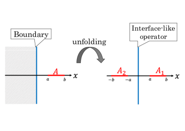
Figure 2: The unfolding process of the boundary state. The kinematics can be fixed by the conformal symmetry of the full plane, called as the doubling trick Cardy (2004).

In CFTs with time-like boundary, the LRMI has a nice picture. Let us consider the LRMI on a half-plane $\Re z>0$ (see the left of FIG. 2). In a similar way to the state-operator correspondence, a conformal boundary can be described by a linear combination of the Ishibashi states Cardy (2004),

$$\ket{B}=\sum_{i}b_{i}\ket{i\rangle}.$$ (4)

The explicit form of the Ishibashi state is

$$\ket{i}\rangle\equiv\sum_{N}\ket{i;N}\otimes U\overline{\ket{i;N}},$$ (5)

where $\ket{i;N}$ is a state in the Verma module $i$ labeled by $N$, and $U$ is an anti-unitary operator. By unfolding the Ishibashi states (which we will denote by $||i||\equiv\sum_{N}\ket{i;N}\otimes U\overline{\bra{i;N}}$), we obtain an interface-like CFT where the interface-like operator $I(B)=\sum_{i}b_{i}||i||$ inserted along the line $z=0$ (see the right of FIG. 2). In this picture, the LRMI is just the mutual information between $A_{1}$ and $A_{2}$ ($A_{i}$ is defined in the right of FIG. 2 ) in this interface-like CFT.

For the later use, we first show the calculation of the LREE for the whole system in our language. The LREE for a system in a strip with size $L$ can be evaluated by the boundary primary correlator with two chiral twist operators,

$$S^{(l/r)}=\lim_{n\to 1}\frac{1}{1-n}\log\frac{\braket{\sigma^{b}_{n}(0)\bar{\sigma}^{b}_{n}(L)}_{strip}}{\braket{\mathbb{I}}_{strip}^{n},}$$ (6)

where we denote the boundary primary by the superscript $b$. The coefficient of the two-point function can be evaliated by the conformal map to a cylinder Das and Datta (2015) as

$$\alpha_{\sigma_{n}^{b}}\equiv\frac{\sum_{i}\left|b_{i}\right|^{2n}S_{i0}}{\left(\sum_{i}\left|b_{i}\right|^{2}S_{i0}\right)^{n}},$$ (7)

where $S_{ij}$ is the modular S matrix and $h_{n}$ is the conformal dimension of the twist operator $h_{n}\equiv\frac{c}{24}\left(n-\frac{1}{n}\right)$. While one sometimes includes the cutoff parameter $\epsilon^{2h_{n}}$ into the coefficient, we split this contribution from the coefficient in this article. For example, in a diagonal RCFT, we obtain

$$S^{(l/r)}=\frac{c}{6}\log\frac{L}{\epsilon}-\left(\sum_{i}S_{ai}^{2}\log\frac{S_{ai}^{2}}{S_{0i}}\right),$$ (8)

where we label the Cardy state by $a$. The constant term is called the topological entanglement entropy. For special boundary states, the same constant term can also be found in (2+1)-$d$ TQFTs as the topological entanglement entropy Das and Datta (2015).

Let us move on to the LREE for a subsystem $A=[a,b]$, that is, the LRMI. Except for some special models, the calculation of the LRMI is difficult. To show a concrete calculation of the LRMI, we focus on the holographic CFT. The entropy $S(A)$ can be evaluated by a correlation function of four chiral twist operators with the interface-like operator $I(B)$,

$$\braket{\bar{\sigma}_{n}(\bar{z}_{1})\sigma_{n}(\bar{z}_{2})I(B)\sigma_{n}(z_{1})\bar{\sigma}_{n}(z_{2})}.$$ (9)

This correlation function can be expanded as

$$g^{n}\sum_{P}C_{\sigma_{n}P}^{2}\mathcal{F}^{Vir}_{P}(1-z),$$ (10)

where the sum runs over boundary primaries and $\mathcal{F}^{Vir}_{P}(z)$ is the Virasoro block with the cross ratio $z\equiv\frac{z_{12}z_{34}}{z_{13}z_{24}}$. The $g$-function represents a disk partition function . In this holographic CFT, the sum can be approximated by just the vacuum block if $z$ is enough large. The bulk-boundary OPE coefficient $C_{\sigma_{n}\mathbb{I}}^{2}$ can be evaluated by the unwrapping procedure Lunin and Mathur (2001). Note that the unwrapping procedure dose not change the profile of the boundary Akal et al. (2021b). The entropy $S^{(L)}_{A}$ is completely fixed by the conformal symmetry. As a result, we obtain

$$I^{(l/r)}(A)=\max\left(\frac{c}{6}\log\frac{(b-a)^{2}}{4ab}-2\log g,0\right).$$ (11)

The trivial case, $I^{(l/r)}(A)=0$, is given by the vacuum block approximation of the dual-channel.

III Left-Right Reflected Entropy

In a similar way to the LRMI, one can introduce another related quantity, left-right reflected entropy (LRRE), which is a generalization of reflected entropy introduced in Dutta and Faulkner (2021) (a similar notion was introduced in Chern-Simons theories Berthiere et al. (2021)). To define the LRRE, we consider a canonical purification of a state $\rho_{A}$ in a doubled Hilbert space $\mathcal{H}_{A}\otimes\mathcal{H}^{*}_{A}$. The LRRE is defined by the reduced density matrix obtained from the purified state $\ket{\sqrt{\rho_{A}}}$ by tracing over the right moving sector,

$$S^{(l/r)}_{R}(A)\equiv-{\text{tr}}\rho^{(L)}_{AA^{*}}\log\rho^{(L)}_{AA^{*}},$$ (12)

where $\rho^{(L)}_{AA^{*}}$ is the reduced density matrix of $\rho_{AA^{*}}=\ket{\sqrt{\rho_{A}}}\bra{\sqrt{\rho_{A}}}$ after tracing over the right moving sector. The physical interpretation of the LRRE is similar to the LRMI. For example, if one evaluates the LRRE in an integrable system, the LRRE behaves in the same way as the LRMI shown in FIG.1. Nevertheless, if one focuses on a non-equilibrium process in a chaotic system where the quasi-particle picture breaks down, the LRRE shows a behavior different from the LRMI (see Kusuki and Tamaoka (2021, 2020); Kudler-Flam et al. (2021, 2020)).

Let us focus on CFTs with time-like boundary at $z=0$. To calculate the LRRE, we can employ the replica trick in the path integral formalism as in Calabrese and Cardy (2004). In the same way as the LRMI, we define the corresponding replica manifold in BCFTs by unfolding (see FIG.2). This replica manifold is shown in FIG. 3, The reflected entropy can be evaluated by the partition function on this replica manifold $Z_{n,m}$ as

$$S^{(l/r)}_{R}(A)=\lim_{n,m\to 1}\frac{1}{1-n}\log\frac{Z_{n,m}}{\left(Z_{1,m}\right)^{n}},$$ (13)

where the analytic continuation $m\to 1$ is taken for even integer $m$. In a similar way to Dutta and Faulkner (2021), this replica partition function can be re-expressed as a correlation function with four chiral twist operators,

$$Z_{n,m}=\Big{\langle}\sigma_{g_{A}}(-b)\sigma_{g_{A}^{-1}}(-a)I(B)\sigma_{g_{B}}(a)\sigma_{g_{B}^{-1}}(b)\Big{\rangle}_{\text{CFT}^{\otimes mn}},$$ (14)

where we take the interval $B=[a,b]$ and its mirror $A=[-b,-a]$. For the same reason as (9), the correlation function includes the interface-like operator. To avoid unnecessary technicalities, we do not show the precise definition of the twist operators $\sigma_{g_{A}}$ and $\sigma_{g_{B}}$ (see Dutta and Faulkner (2021)) because in this article, we only use the conformal dimension of the twist operators,

$$h_{\sigma_{g_{A}}}=h_{\sigma_{g_{A}^{-1}}}=h_{\sigma_{g_{B}}}=h_{\sigma_{g_{B}^{-1}}}=\frac{cn}{24}\left(m-\frac{1}{m}\right)(=nh_{m}),$$ (15)

$$h_{\sigma_{g_{A}^{-1}g_{B}}}=h_{\sigma_{g_{B}^{-1}g_{A}}}=\frac{c}{12}\left(n-\frac{1}{n}\right)(=2h_{n}),$$

where $h_{\sigma_{g_{A}^{-1}g_{B}}}$ ($h_{\sigma_{g_{B}^{-1}g_{A}}}$) appears as the conformal dimension of the lowest primary operator in the OPE between $\sigma_{g_{A}^{-1}}$ and $\sigma_{g_{B}}$ ( $\sigma_{g_{B}^{-1}}$ and $\sigma_{g_{A}}$ ).

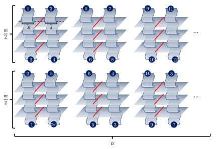
Figure 3: The replica manifold that calculates the reflected entropy. Edges labeled with the same number get glued together. The red lines describe the interface-like operators.

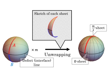
Figure 4: Sketch of how to evaluate the OPE coefficient. We can unwrap the $m$-fold branch cut by the conformal transformation $z\to z^{\frac{1}{m}}$. This unwrapping leads to a sphere with one interface line (black line) and the $n$-fold branch cut (red line), whose edge is attached to the interface. This is completely the same as the setup studied in Sakai and Satoh (2008); Brehm and Brunner (2015). Using the technique in Sakai and Satoh (2008); Brehm and Brunner (2015), one can evaluate this partition function.

The reflected entropy has a nice bulk interpretation. One can show that the reflected entropy is dual to twice the area of the entanglement wedge cross section, $S_{R}=2E_{W}$ Dutta and Faulkner (2021). In a similar way, one can find the holographic dual of the LRRE. In the holographic CFT, the correlation function (14) in the limits $n\to 1$ and $m\to 1$ can be approximated by a single Virasoro block $\mathcal{F}^{Vir}(2h_{n}|1-z)$ if $z$ is enough large and then we have

$$\frac{Z_{n,m}}{\left(Z_{1,m}\right)^{n}}=\alpha_{\sigma_{n}^{b}}^{-2}C_{\sigma_{g_{A}^{-1}}\sigma_{g_{B}}\sigma_{g_{A}g_{B}^{-1}}^{b}}^{2}\left(\frac{1+\sqrt{z}}{2\sqrt{1-z}}\right)^{-4h_{n}}.$$ (16)

The factor $\alpha_{\sigma_{n}^{b}}^{-2}$ comes from the normalization of the twist operator (7). The OPE coefficient $C_{\sigma_{g_{A}^{-1}}\sigma_{g_{B}}\sigma_{g_{A}g_{B}^{-1}}^{b}}$ can be evaluated by the unwrapping trick Lunin and Mathur (2001) (see also Dutta and Faulkner (2021)). Since the unwrapping procedure does not affect the interface, we have

$$C_{\sigma_{g_{A}^{-1}}\sigma_{g_{B}}\sigma_{g_{A}g_{B}^{-1}}^{b}}=\left(2m\right)^{-2h_{n}}\alpha_{\sigma_{n}^{b}},$$ (17)

where $\alpha_{\sigma_{n}^{b}}$ is defined in (7). The reason why we obtain the coefficient $\alpha_{\sigma_{n}^{b}}$ is explained in FIG.4. Thus, the reflected entropy is given by

$$S^{(l/r)}_{R}(A)=\frac{c}{3}\log\left(\frac{b}{a}\right)+const.,$$ (18)

which completely matches twice the area of the entanglement wedge cross section defined in FIG.5 up to constant.

One can also evaluate the LRRE in the adjacent limit. Let us first consider the limit $1-z=\frac{4ab}{(a+b)^{2}}\ll\epsilon\ll 1$. In this case, the replica partition function can be approximated by

$$\frac{Z_{n,m}}{\left(Z_{1,m}\right)^{n}}=C_{\sigma_{g_{A}^{-1}}\sigma_{g_{B}}\sigma_{g_{A}g_{B}^{-1}}^{b}}\left(\frac{(a+b)^{2}}{ab}\right)^{-2h_{n}}.$$ (19)

As a result, the LRRE for the Cardy state $\ket{a}$ in a diagonal RCFT is given by

$$S^{(l/r)}_{R}(A)\to\frac{c}{6}\log{\frac{(a+b)^{2}}{ab}}-2\left(\sum_{i}S_{ai}^{2}\log\frac{S_{ai}^{2}}{S_{0}i}\right).$$ (20)

The second term comes from the coefficient $\alpha_{\sigma_{n}^{b}}$ in (17). On the other hand, if we take the limit $\epsilon\ll 1-z=\frac{4ab}{(a+b)^{2}}\ll 1$, we obtain from (16)

$$S^{(l/r)}_{R}(A)\to\frac{c}{6}\log{\frac{(a+b)^{2}}{ab}}.$$ (21)

In the limit of the adjacent intervals, one can find that the Markov gap Hayden et al. (2021) has the following form,

$$S^{(l/r)}_{R}(A)-I^{(l/r)}_{R}(A)=\frac{c}{3}\log 2+\cdots.$$ (22)

This universal term can also be found in a special tripartition setup Zou et al. (2021). The additional terms $\cdots$ depend on the details of the boundary.

Note that in the holographic CFT, the LRRE for a finite subsystem satisfies the inequality (an analog of Hayden et al. (2021) in CFTs without boundary),

$$S^{(l/r)}_{R}(A)-I^{(l/r)}_{R}(A)\geq\frac{c}{6}\log 2\times(\text{\# of cross section bounraries}).$$ (23)

It is claimed that the reflected entropy is more sensitive to multipartite entanglement Akers and Rath (2020); Zou et al. (2021). The $O(c)$ difference between the reflected entropy and the mutual information implies that there must be a large amount of tripartite entanglement in our tripartition setup associated with the division of the left/right moving sectors.

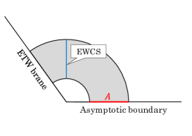
Figure 5: The holographic dual of the LRRE in BCFTs. This is given by the entanglement wedge cross section (EWCS), which is defined in Takayanagi and Umemoto (2018); Nguyen et al. (2018).

IV Reflected Entropy in Interface CFT

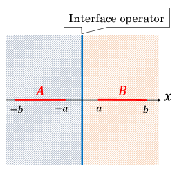
Figure 6: The setup that we consider. The interface is symmetrically localed on the two intervals. One can also consider an asymmetric setup for topological interfaces.

In a similar way to the LRRE, we can define the reflected entropy in an interface CFT, i.e., $\text{CFT}_{1}\otimes\overline{\text{CFT}}_{2}$ with central charge $c_{1}$ and $c_{2}$ (see our setup in FIG.6),

$$S_{R}(A,B)=\lim_{n,m\to 1}\frac{1}{1-n}\log\frac{Z_{n,m}}{\left(Z_{1,m}\right)^{n}},$$ (24)

where the partition function is expressed in terms of (not chiral) twist operators as

$$Z_{n,m}=\Big{\langle}\sigma_{g_{A}}(u_{1})\sigma_{g_{A}^{-1}}(v_{1})I(A)\sigma_{g_{B}}(u_{2})\sigma_{g_{B}^{-1}}(v_{2})\Big{\rangle}_{\text{CFT}^{\otimes mn}},$$ (25)

where we take the intervals $A=[u_{1},v_{1}]$ and $B=[u_{2},v_{2}]$ with $u_{1}<v_{1}<u_{2}<v_{2}$. Since the calculation of the reflected entropy is still difficult in general, we focus on the case where the correlation function is approximated by the single block, as in the holographic CFT or in the limit of the adjacent intervals. In a similar way to the BCFT case, one may approximate the correlation function in the holographic CFT as

$$\frac{Z_{n,m}}{\left(Z_{1,m}\right)^{n}} =C_{\sigma_{g_{A}^{-1}}\sigma_{g_{B}}\sigma_{g_{A}g_{B}^{-1}}^{b}}^{2}\left|\mathcal{F}^{Vir}(2h^{\prime}_{n}|1-z)\right|^{2},$$ (26)

where $h^{\prime}_{n}\equiv\frac{c_{\text{eff}}}{24}\left(n-\frac{1}{n}\right)$ and

$$C_{\sigma_{g_{A}^{-1}}\sigma_{g_{B}}\sigma_{g_{A}g_{B}^{-1}}^{b}}=\left(2m\right)^{-4h_{n}}\alpha_{\sigma_{n}^{b}}^{2},$$ (27)

where the twist operator is not a chiral twist operator unlike that in (6). This is true for topological defects but in general, could not be true. This is because one cannot organize the descendant contributions in the same way as CFT without defects. One thing we can say for sure is that the leading contribution in the limit of the adjacent intervals $z\to 1$ is given by

$$\frac{Z_{n,m}}{\left(Z_{1,m}\right)^{n}} =\alpha_{\sigma_{n}^{b}}^{-2}C_{\sigma_{g_{A}^{-1}}\sigma_{g_{B}}\sigma_{g_{A}g_{B}^{-1}}^{b}}^{2}\left|(1-z)^{2h^{\prime}_{n}}\right|^{2}.$$ (28)

The effective central charge $c_{\text{eff}}\in[0,\min(c_{1},c_{2})]$ depends on a profile of the interface (see Sakai and Satoh (2008)). Consequently, the reflected entropy in the limit of the adjacent intervals $1-z=\frac{4ab}{(a+b)^{2}}\ll 1$ is given by

$$S_{R}(A,B)=\frac{c_{\text{eff}}}{3}\log{\frac{(a+b)^{2}}{ab}}+const..$$ (29)

The OPE coefficient can be obtained by the unwrapping procedure (see FIG.4). For the same reason as the entanglement entropy, it is difficult to evaluate the OPE coefficient (more precisely, an analog of $\alpha_{\sigma_{n}^{b}}$) in generic interface CFTs. Nevertheless, in a specific case, topological interface, we can give the explicit form of the constant part in a similar way as the LRRE in BCFTs. (See Brehm et al. (2016) for the derivation of $\alpha_{\sigma_{n}^{b}}$ and its interpretation.) For topological interfaces, the Markov gap is given by

$$S_{R}(A,B)-I(A,B)=\frac{2c}{3}\log 2+\cdots.$$ (30)

The additional terms $\cdots$ depend on the details of the interface. This universal term is completely consistent with Zou et al. (2021). In general interfaces, the Markov has a complicated form. We provide further analysis in Liu et al. .

Let us focus on the holographic interface. One natural realization of the holographic dual of the interface CFT is given by the so-called Janus solution Bachas et al. (2002); Bak et al. (2003, 2007). The entanglement entropy in this holographic interface is evaluated in various setups Azeyanagi et al. (2008); Gutperle and Miller (2016b); Karch et al. (2021). In a similar way to Azeyanagi et al. (2008); Gutperle and Miller (2016b); Karch et al. (2021), the entanglement wedge cross section can be evaluated. In the case considered in Karch et al. (2021) (also in Azeyanagi et al. (2008); Gutperle and Miller (2016b)), the reflected entropy is given by

$$S_{R}(A,B)=\frac{2c_{\text{eff}}}{3}\log\left(\frac{b}{a}\right)+const..$$ (31)

The effective central charge is the same as that found in Gutperle and Miller (2016b).

There is another realization by simply connecting two geometries by a thin brane Azeyanagi et al. (2008); Karch et al. (2021); Erdmenger et al. (2015); Simidzija and Van Raamsdonk (2020); Bachas et al. (2020, 2021); Bachas and Papadopoulos (2021); Anous et al. (2022), which is a generalization of the bottom-up AdS/BCFT Takayanagi (2011); Fujita et al. (2011). Although there is limited knowledge about the CFT dual of this model, this model is interesting for two reasons. Unlike the top-down model, the thin-brane model is a minimal gravity dual of ICFT. This is an analog of pure gravity. Another reason comes from the island model Penington (2020); Almheiri et al. (2019); Almheiri et al. (2020a). One can think of the thin-brane as a gravity theory coupled to a non-gravitational bath CFT, called the braneworld holography Karch and Randall (2001). Through this holography, one can investigate the island model by the ICFT dual to the thin-brane model. In the thin-brane model, the minimal cross section of the entanglement wedge is given by

$$S_{R}(A,B)=\frac{2\min(c_{1},c_{2})}{3}\log\left(\frac{b}{a}\right)+const..$$ (32)

This form of the reflected entropy is non-trivial as we mentioned below (26). This may strongly constrain the profile of the holographic interface.

V Discussions

In this article, we develop the idea of reflected entropy in BCFT/ICFT. We propose some remaining questions and interesting future works. It would be interesting to investigate the reflected entropy in various setups with boundaries or interfaces, which would tell us about the multipartite entanglement between bulk and boundary/interface. In the holographic CFT, one can explicitly evaluate the reflected entropy in BCFT/ICFT, which has the potential to identify the profile of the holographic interface in the CFT language. An interesting future work is to apply our analysis to the island model, which is essentially a special class of BCFT/ICFT. From such an analysis, one may be able to understand the multipartite entanglement structure of the island model. It is known that the LREE in (1+1)-$d$ CFT has a nice interpretation in (2+1)-$d$ TQFT Das and Datta (2015); Berthiere et al. (2021); Nishioka et al. (2021). It would be interesting to find the TQFT picture of the LRRE.

References

- Ryu and Takayanagi (2006) S. Ryu and T. Takayanagi, JHEP 08, 045 (2006), eprint hep-th/0605073.
- Dutta and Faulkner (2021) S. Dutta and T. Faulkner, JHEP 03, 178 (2021), eprint 1905.00577.
- Kudler-Flam et al. (2021) J. Kudler-Flam, Y. Kusuki, and S. Ryu, JHEP 03, 146 (2021), eprint 2008.11266.
- Kudler-Flam et al. (2020) J. Kudler-Flam, Y. Kusuki, and S. Ryu, JHEP 04, 074 (2020), eprint 2001.05501.
- Kusuki and Tamaoka (2021) Y. Kusuki and K. Tamaoka, Phys. Lett. B 814, 136105 (2021), eprint 1907.06646.
- Kusuki and Tamaoka (2020) Y. Kusuki and K. Tamaoka, JHEP 02, 017 (2020), eprint 1909.06790.
- Bueno and Casini (2020a) P. Bueno and H. Casini, JHEP 05, 103 (2020a), eprint 2003.09546.
- Zou and Vidal (2022) Y. Zou and G. Vidal, Phys. Rev. B 105, 125125 (2022), eprint 2108.09366.
- Liu et al. (2022) Y. Liu, R. Sohal, J. Kudler-Flam, and S. Ryu, Phys. Rev. B 105, 115107 (2022), eprint 2110.11980.
- Siva et al. (2021) K. Siva, Y. Zou, T. Soejima, R. S. K. Mong, and M. P. Zaletel (2021), eprint 2110.11965.
- Berthiere et al. (2021) C. Berthiere, H. Chen, Y. Liu, and B. Chen, Phys. Rev. B 103, 035149 (2021), eprint 2008.07950.
- Bueno and Casini (2020b) P. Bueno and H. Casini, JHEP 11, 148 (2020b), eprint 2008.11373.
- Camargo et al. (2021) H. A. Camargo, L. Hackl, M. P. Heller, A. Jahn, and B. Windt, Phys. Rev. Lett. 127, 141604 (2021), eprint 2102.00013.
- Akers and Rath (2020) C. Akers and P. Rath, JHEP 04, 208 (2020), eprint 1911.07852.
- Zou et al. (2021) Y. Zou, K. Siva, T. Soejima, R. S. K. Mong, and M. P. Zaletel, Phys. Rev. Lett. 126, 120501 (2021), eprint 2011.11864.
- Note (1) Note1, more precisely, implies no W-like entanglement. It does not imply no GHZ entanglement.
- Hayden et al. (2021) P. Hayden, O. Parrikar, and J. Sorce, JHEP 10, 047 (2021), eprint 2107.00009.
- Cardy (2004) J. L. Cardy (2004), eprint hep-th/0411189.
- Pando Zayas and Quiroz (2015) L. A. Pando Zayas and N. Quiroz, JHEP 01, 110 (2015), eprint 1407.7057.
- Das and Datta (2015) D. Das and S. Datta, Phys. Rev. Lett. 115, 131602 (2015), eprint 1504.02475.
- Affleck et al. (2009) I. Affleck, N. Laflorencie, and E. S. Sorensen, J. Phys. A: Math. Theor. 42 504009 (2009) (2009), eprint 0906.1809.
- Oshikawa and Affleck (1996) M. Oshikawa and I. Affleck, Phys. Rev. Lett. 77, 2604 (1996), eprint hep-th/9606177.
- Oshikawa and Affleck (1997) M. Oshikawa and I. Affleck, Nucl. Phys. B 495, 533 (1997), eprint cond-mat/9612187.
- Bachas et al. (2002) C. Bachas, J. de Boer, R. Dijkgraaf, and H. Ooguri, JHEP 06, 027 (2002), eprint hep-th/0111210.
- Sakai and Satoh (2008) K. Sakai and Y. Satoh, JHEP 12, 001 (2008), eprint 0809.4548.
- Brehm and Brunner (2015) E. M. Brehm and I. Brunner, JHEP 09, 080 (2015), eprint 1505.02647.
- Brehm et al. (2016) E. M. Brehm, I. Brunner, D. Jaud, and C. Schmidt-Colinet, Fortsch. Phys. 64, 516 (2016), eprint 1512.05945.
- Wen et al. (2018) X. Wen, Y. Wang, and S. Ryu, J. Phys. A 51, 195004 (2018), eprint 1711.02126.
- Gutperle and Miller (2016a) M. Gutperle and J. D. Miller, JHEP 04, 176 (2016a), eprint 1512.07241.
- (30) Y. Liu, R. Sohal, Y. Kusuki, J. Kudler-Flam, and S. Ryu, work in progress (????).
- Penington (2020) G. Penington, JHEP 09, 002 (2020), eprint 1905.08255.
- Almheiri et al. (2019) A. Almheiri, N. Engelhardt, D. Marolf, and H. Maxfield, JHEP 12, 063 (2019), eprint 1905.08762.
- Almheiri et al. (2020a) A. Almheiri, R. Mahajan, J. Maldacena, and Y. Zhao, JHEP 03, 149 (2020a), eprint 1908.10996.
- Almheiri et al. (2020b) A. Almheiri, R. Mahajan, and J. E. Santos, SciPost Phys. 9, 001 (2020b), eprint 1911.09666.
- Sully et al. (2021) J. Sully, M. V. Raamsdonk, and D. Wakeham, JHEP 03, 167 (2021), eprint 2004.13088.
- Akal et al. (2020) I. Akal, Y. Kusuki, T. Takayanagi, and Z. Wei, Phys. Rev. D 102, 126007 (2020), eprint 2007.06800.
- Bousso and Wildenhain (2020) R. Bousso and E. Wildenhain, Phys. Rev. D 102, 066005 (2020), eprint 2006.16289.
- Miao (2021) R.-X. Miao, JHEP 01, 150 (2021), eprint 2009.06263.
- Akal et al. (2021a) I. Akal, Y. Kusuki, N. Shiba, T. Takayanagi, and Z. Wei, Phys. Rev. Lett. 126, 061604 (2021a), eprint 2011.12005.
- Geng and Karch (2020) H. Geng and A. Karch, JHEP 09, 121 (2020), eprint 2006.02438.
- Geng et al. (2021a) H. Geng, A. Karch, C. Perez-Pardavila, S. Raju, L. Randall, M. Riojas, and S. Shashi, SciPost Phys. 10, 103 (2021a), eprint 2012.04671.
- Chu et al. (2021) J. Chu, F. Deng, and Y. Zhou, JHEP 10, 149 (2021), eprint 2105.09106.
- Akal et al. (2021b) I. Akal, Y. Kusuki, N. Shiba, T. Takayanagi, and Z. Wei, Class. Quant. Grav. 38, 224001 (2021b), eprint 2106.11179.
- Ageev (2021) D. S. Ageev (2021), eprint 2107.09083.
- Geng et al. (2021b) H. Geng, A. Karch, C. Perez-Pardavila, S. Raju, L. Randall, M. Riojas, and S. Shashi (2021b), eprint 2112.09132.
- Kusuki (2022a) Y. Kusuki, JHEP 03, 161 (2022a), eprint 2112.10984.
- Suzuki and Takayanagi (2022) K. Suzuki and T. Takayanagi (2022), eprint 2202.08462.
- Numasawa and Tsiares (2022) T. Numasawa and I. Tsiares (2022), eprint 2202.01633.
- Izumi et al. (2022) K. Izumi, T. Shiromizu, K. Suzuki, T. Takayanagi, and N. Tanahashi (2022), eprint 2205.15500.
- Kusuki (2022b) Y. Kusuki (2022b), eprint 2206.03035.
- Akers et al. (2022) C. Akers, T. Faulkner, S. Lin, and P. Rath (2022), eprint 2201.11730.
- Chandrasekaran et al. (2020) V. Chandrasekaran, M. Miyaji, and P. Rath, Phys. Rev. D 102, 086009 (2020), eprint 2006.10754.
- Li et al. (2020) T. Li, J. Chu, and Y. Zhou, JHEP 11, 155 (2020), eprint 2006.10846.
- Ghodrati (2021) M. Ghodrati (2021), eprint 2110.12970.
- Note (2) Note2, we can formally define the chiral twist operator by the unwrapping Lunin and Mathur (2001). For example, the OPE coefficients including the chiral twist operators are evaluated by this prescription. See also Hoogeveen and Doyon (2015).
- Note (3) Note3, this -function is not defined in the orbifold CFT but in the seed CFT .
- Lunin and Mathur (2001) O. Lunin and S. D. Mathur, Commun. Math. Phys. 219, 399 (2001), eprint hep-th/0006196.
- Calabrese and Cardy (2004) P. Calabrese and J. L. Cardy, J. Stat. Mech. 0406, P06002 (2004), eprint hep-th/0405152.
- Takayanagi and Umemoto (2018) T. Takayanagi and K. Umemoto, Nature Phys. 14, 573 (2018), eprint 1708.09393.
- Nguyen et al. (2018) P. Nguyen, T. Devakul, M. G. Halbasch, M. P. Zaletel, and B. Swingle, JHEP 01, 098 (2018), eprint 1709.07424.
- Note (4) Note4, this conformal dimension can be obtained by evaluating the vacuum energy of the closed string sector of the cylinder partition function associated with the replica manifold shown in the right of FIG.4. The same technique can be found in Sakai and Satoh (2008); Brehm and Brunner (2015).
- Bak et al. (2003) D. Bak, M. Gutperle, and S. Hirano, JHEP 05, 072 (2003), eprint hep-th/0304129.
- Bak et al. (2007) D. Bak, M. Gutperle, and S. Hirano, JHEP 02, 068 (2007), eprint hep-th/0701108.
- Azeyanagi et al. (2008) T. Azeyanagi, A. Karch, T. Takayanagi, and E. G. Thompson, JHEP 03, 054 (2008), eprint 0712.1850.
- Gutperle and Miller (2016b) M. Gutperle and J. D. Miller, Phys. Rev. D 93, 026006 (2016b), eprint 1511.08955.
- Karch et al. (2021) A. Karch, Z.-X. Luo, and H.-Y. Sun, JHEP 09, 172 (2021), eprint 2107.02165.
- Erdmenger et al. (2015) J. Erdmenger, M. Flory, and M.-N. Newrzella, JHEP 01, 058 (2015), eprint 1410.7811.
- Simidzija and Van Raamsdonk (2020) P. Simidzija and M. Van Raamsdonk, JHEP 12, 028 (2020), eprint 2006.13943.
- Bachas et al. (2020) C. Bachas, S. Chapman, D. Ge, and G. Policastro, Phys. Rev. Lett. 125, 231602 (2020), eprint 2006.11333.
- Bachas et al. (2021) C. Bachas, Z. Chen, and V. Papadopoulos, JHEP 11, 095 (2021), eprint 2107.00965.
- Bachas and Papadopoulos (2021) C. Bachas and V. Papadopoulos, JHEP 04, 262 (2021), eprint 2101.12529.
- Anous et al. (2022) T. Anous, M. Meineri, P. Pelliconi, and J. Sonner (2022), eprint 2202.11718.
- Takayanagi (2011) T. Takayanagi, Phys. Rev. Lett. 107, 101602 (2011), eprint 1105.5165.
- Fujita et al. (2011) M. Fujita, T. Takayanagi, and E. Tonni, JHEP 11, 043 (2011), eprint 1108.5152.
- Karch and Randall (2001) A. Karch and L. Randall, JHEP 05, 008 (2001), eprint hep-th/0011156.
- Nishioka et al. (2021) T. Nishioka, T. Takayanagi, and Y. Taki, JHEP 09, 015 (2021), eprint 2107.01797.
- Hoogeveen and Doyon (2015) M. Hoogeveen and B. Doyon, Nucl. Phys. B 898, 78 (2015), eprint 1412.7568.