On retrograde orbits, resonances and stability

Abstract

We start by reviewing our previous work on retrograde orbital configurations and on modeling and identifying retrograde resonances. Then, we present new results regarding the enhanced stability of retrograde configurations with respect to prograde configurations in the low mass ratio regime of the planar circular restricted 3-body problem. Motivated by the recent discovery of small bodies which are in retrograde resonance with the Solar System’s giant planets we then explore the case with mass ratio $0.001$ and show new stability maps in a grid of semi-major axis versus eccentricity for the 2/1 and 1/2 retrograde resonances. Finally, we explain how the stability borders of the 2/1 and 1/2 retrograde resonances are related to the resonant orbits’ geometry.

1 Introduction

A retrograde orbital configuration consists of two or more bodies moving around a central mass in opposite directions or, more precisely, such that the relative inclination $180^{\circ}\geq I>90^{\circ}$. When $I=180^{\circ}$ the orbits are retrograde and coplanar.

Examples of retrograde orbital motion in the Solar System include: many comets, 63 small bodies including Mars crossing asteroids, a subset of Centaurs called Damocloids, a TNO (2008KV42), and distant objects on nearly parabolic orbits. Many irregular satellites of the giant planets and Neptune’s moon Triton also have retrograde orbital motion. Extrasolar planetary systems are detected through indirect methods and the relative inclinations are usually not known. Retrograde configurations could be achieved e.g.  through capture of a free floating planet in a star cluster which has isotropic probability Perets2012ApJ , Varvoglis2012CeMDA .

Analysis of radial velocity data for the star $\nu$-Octantis A by Ramm_etal2009MNRAS led to the claim that there is a planet about half-way between $\nu$-Octantis A and its binary companion, $\nu$-Octantis B. This result was puzzling since a planet at such location in a prograde configuration would be unstable due to the strong perturbation from $\nu$-Octantis B and led to alternative hypothesis for this system Morais&Correia2012MNRAS . Numerical integrations by Eberle&Cuntz2010ApJ and Gozdziewski2013MNRAS showed that a planet in a retrograde configuration could be stable in the $\nu$-Octantis system which prompted a study of the stability of retrograde configurations in binary systems by Morais&Giuppone2012MNRAS . This showed that the enhanced stability of retrograde configurations with respect to prograde configurations is due to the nature of retrograde resonances which are weaker than prograde resonances at a given orbital period ratio Morais&Giuppone2012MNRAS .

In Morais&Namouni2013CMDA we studied retrograde resonance in the framework of the circular restricted 3-body problem (CR3BP), identifying the relevant resonant arguments in the disturbing function and exploring retrograde resonance stability using the method of surfaces of section. In Morais&Namouni2013MNRASL we identified small bodies (Damocloids) which are currently in the 1/2 and 2/5 retrograde resonances with Jupiter, and in the 2/3 retrograde resonance with Saturn. In Namouni&Morais2015MNRAS we performed a numerical study of the resonance capture probabilities for objects on prograde and retrograde orbits migrating inwards towards a Jupiter mass planet. We saw that capture in resonance is more likely for retrograde inclinations ($I>90^{\circ}$) rather than prograde inclinations ($I<90^{\circ}$).

This article is organized as follows: In Sect. 2 we review our work on the retrograde disturbing function, explain how to obtain retrograde resonance’s critical angles and associated resonance strength. In Sect. 3 we present results on the enhanced stability of retrograde configurations with respect to prograde configurations for mass ratio $<0.01$ relevant for planetary systems. In Sect. 4 we show stability maps in a grid of semi-major axis versus eccentricity for the 2/1 and 1/2 retrograde resonances. In Sect. 5 we discuss our results.

2 Retrograde resonance

2.1 Retrograde and prograde disturbing functions

Consider the restricted 3-body problem consisting of a test particle subject to the gravitational influence of a primary and secondary (mass ratio $\mu$) which are on circular orbit of unit radius (CR3BP). The disturbing function is

$$R=\mu\left(\frac{1}{\Delta}-r\cos{\psi}\right)$$ (1)

where $r$ is the radial distance to the primary, $\Delta=\sqrt{1+r^{2}-2\,r\,\cos{\psi}}$,

$$\cos\psi = \cos(f+\omega)\cos(\Omega-\lambda^{\prime})-\sin(f+\omega)\sin(\Omega-\lambda^{\prime})\cos{I}$$ (2)

$$= \cos^{2}(I/2)\cos(f+\omega+\Omega-\lambda^{\prime})+\sin^{2}(I/2)\cos(f+\omega-\Omega+\lambda^{\prime})\ .$$

If the orbit is prograde with inclination $I\approx 0$ then $\sin^{2}(I/2)\ll 1$ hence we define a small parameter

$$\Psi=\cos{\psi}-\cos(f+\omega+\Omega-\lambda^{\prime})=2\,\sin^{2}(I/2)\sin(\Omega-\lambda^{\prime})\sin(\omega+f)\ ,$$ (3)

and expanding the indirect term of Eq. (1) around $\Psi=0$ leads to the classical expression ssdbook

$$\frac{1}{\Delta} = \sum_{i=0}^{\infty}\frac{(2i)!}{(i!)^{2}}\left(\frac{1}{2}r\Psi\right)^{i}\frac{1}{\Delta_{0}^{2\,i+1}}$$ (4)

with $\Delta_{0}=\sqrt{1+r^{2}-2\,r\,\cos(f+\omega+\Omega-\lambda^{\prime})}$.

If the orbit is retrograde with inclination $I\approx 180^{\circ}$ then $\cos^{2}(I/2)\ll 1$ hence $\Psi\gg 1$ and the expansion in Eq. 4 is not valid. Following Morais&Namouni2013CMDA we define a small parameter

$$\bar{\Psi}=\cos{\psi}-\cos(f+\omega-\Omega+\lambda^{\prime})=2\,\cos^{2}(I/2)\sin(-\Omega+\lambda^{\prime})\sin(\omega+f)\ ,$$ (5)

and expanding the indirect term of Eq. (1) around $\bar{\Psi}=0$ leads to

$$\frac{1}{\Delta} = \sum_{i=0}^{\infty}\frac{(2i)!}{(i!)^{2}}\left(\frac{1}{2}r\bar{\Psi}\right)^{i}\frac{1}{\bar{\Delta}_{0}^{2\,i+1}}$$ (6)

with $\bar{\Delta}_{0}=\sqrt{1+r^{2}-2\,r\,\cos(f+\omega-\Omega+\lambda^{\prime})}$.

Therefore, we see that the expansions of the disturbing function for prograde (Eq. 4) and retrograde (Eq. 6) orbits are related. The latter may be obtained from the former by performing the following canonical transformation Morais&Namouni2013CMDA

$$\parbox{56.9055pt}{$I^{\star}=180^{\circ}-I$}\quad\quad\parbox{56.9055pt}{$\lambda^{\prime\star}=-\lambda^{\prime}$}\quad\parbox{56.9055pt}{$\omega^{\star}=\omega-\pi$}\quad\parbox{56.9055pt}{$\Omega^{\star}=-\Omega-\pi$}\ .$$ (7)

The canonical transformation (Eq. 7) has a physical meaning: it is analogous to obtaining a retrograde orbit of inclination $I$ from a prograde orbit of inclination $180^{\circ}-I$ by simply inverting the motion of the massive bodies. This is the 3D version of the procedure described in Morais&Giuppone2012MNRAS to obtain the retrograde disturbing function from the prograde disturbing function in the planar (2D) problem.

2.2 Retrograde resonance critical angles

By inspection of the disturbing function’s expansion (Eq. 6) we conclude that at the $p/q$ retrograde resonance the slow terms are

$$e^{p+q-2\,k}\cos^{2\,k}(I/2)\cos(q\,\lambda^{\star}+p\,\lambda^{\prime\star}-(p+q-2\,k)\varpi^{\star}-2\,k\,\Omega^{\star})$$ (8)

with $2\,k\leq p+q$, $\lambda^{\star}=\lambda-2\,\Omega$, $\varpi^{\star}=\omega-\Omega=\varpi-2\,\Omega$.

As an example we discuss the case of the 2/1 and 1/2 resonances. The 2/1 (1/2) prograde resonance has critical angle $\lambda-2\,\lambda^{\prime}+\varpi$ ($2\,\lambda-\lambda^{\prime}-\varpi$), which appears at 1st order in eccentricity i.e. the amplitude (or strength) of the resonance term is ${\cal O}(e)$, while the 2/1 and 1/2 retrograde resonances have 2 critical angles each which appear at 3rd order in eccentricity and inclination. The 2/1 retrograde resonance has critical angles:

• $\phi^{\star}_{21}=\lambda^{\star}+2\,\lambda^{\prime\star}-3\,\varpi^{\star}=\lambda-2\,\lambda^{\prime}-3\,\varpi+4\,\Omega$,     ${\cal O}(e^{3})$;

• $\phi^{\star}_{21}=\lambda^{\star}+2\,\lambda^{\prime\star}-\varpi^{\star}-2\,\Omega^{\star}=\lambda-2\,\lambda^{\prime}-\varpi+2\,\Omega$,  ${\cal O}(e\cos^{2}(I/2))$;

while the 1/2 retrograde resonance has critical angles:

• $\phi^{\star}_{12}=2\,\lambda^{\star}+\lambda^{\prime\star}-3\,\varpi^{\star}=2\,\lambda-\lambda^{\prime}-3\,\varpi+2\,\Omega$     ${\cal O}(e^{3})$, ;

• $\phi^{\star}_{12}=2\,\lambda^{\star}+\lambda^{\prime\star}-\varpi^{\star}-2\,\Omega^{\star}=2\,\lambda-\lambda^{\prime}-\varpi$,    ${\cal O}(e\cos^{2}(I/2))$.

In the planar (2D) problem the 2/1 and 1/2 retrograde resonances have single critical angles, $\phi^{\star}_{21}=\lambda^{\star}-2\,\lambda^{\prime}-3\,\varpi^{\star}$ and $\phi^{\star}_{12}=2\,\lambda^{\star}-\lambda^{\prime}-3\,\varpi^{\star}$, respectively. Fig. 1 shows planar orbits in the 2/1 retrograde resonance corresponding to libration of $\phi^{\star}_{21}$ around 0 or $180^{\circ}$. Fig. 2 shows planar orbits in the 1/2 retrograde resonance corresponding to libration of $\phi^{\star}_{12}$ around 0 or $180^{\circ}$. The location of the resonances’ centers at a given mass ratio $\mu$ depends on $a$ and $e$ as we will confirm in Sect. 4.

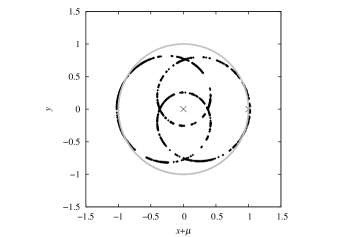
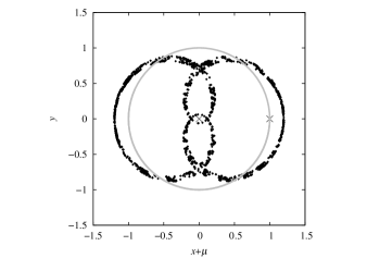
Figure 1: Orbits in 2/1 retrograde resonance (CR3BP with mass ratio $\mu=0.001$): libration around 0 (left) with $a=0.63$ and $e=0.8$ (top) or $e=0.4$ (low); libration around $180^{\circ}$ (right) with $a=0.64$ and $e=0.6$ (top) or $a=0.63$ and $e=0.9$ (low). The star and planet are identified by symbol $\times$ at $(0,0)$ and $(1,0)$ and the gray circle has unit radius.

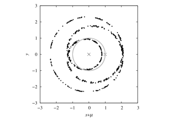
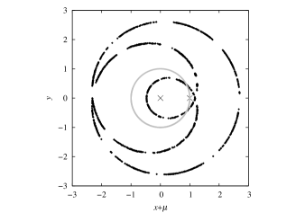
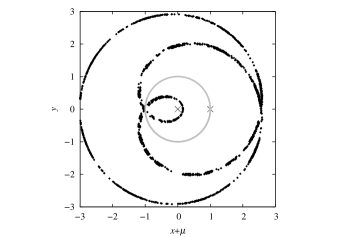
Figure 2: Orbits in 1/2 retrograde resonance (CR3BP with mass ratio $\mu=0.001$): libration around 0 (left) with $a=1.6$ and $e=0.5$ (top) or $a=1.59$ and $e=0.9$ (low); libration around $180^{\circ}$ (right) with $a=1.59$ and $e=0.7$ (top) or $e=0.3$ (low). The star and planet are identified by symbol $\times$ at $(0,0)$ and $(1,0)$ and the gray circle has unit radius.

3 Enhanced stability of retrograde configurations

In Morais&Giuppone2012MNRAS we showed that a planet orbiting the primary star of a binary may be stable closer to the secondary star if it has a retrograde orbit rather than a prograde orbit. We explained that this is due to retrograde resonances being weaker than prograde resonances, i.e. at a given mean motion ratio $p/q$, prograde resonances are of order $p-q$ while retrograde resonances are of order $p+q$. This has two effects on stability: 1) the excitation of eccentricity is smaller for retrograde resonances; 2) the overlap of resonances which generates a chaotic layer in the vicinity of the secondary Wisdom1980AJ is less widespread for retrograde configurations. This can also be understood in terms of the effect of close encounters with the secondary which generate the chaotic layer in its vicinity. Close encounters in retrograde configurations occur at larger relative velocity (hence have shorter duration and consequentely are less disruptive to the orbit) than in prograde configurations.

In Morais&Giuppone2012MNRAS we were interested in the high mass ratio regime and inner orbits, relevant for studying the stability of a planet around the primary star of a binary system. Here, we revisit the problem of stability concentrating in the low mass ratio regime ($\mu<0.01$) and both inner and outer orbits. This is relevant for a small body (test particle) orbiting a star subject to the perturbation by a nearby planet (mass ratio $\mu$). We numerically integrate the equations of motion of the CR3BP, together with the variational equations and MEGNO equations Cincotta2000 ; Gozdziewski2003A&A for $5\,\times 10^{4}$ binary’s periods.

In Fig. 3 we show the MEGNO maps for retrograde (top panel) and prograde (low panel) configurations in a grid of semi-major axis $1.2\geq a\geq 0.8$ varying at steps $0.05\,R_{H}$, and mass ratio $0.01\geq\mu\geq 0.0001$ varying at steps $0.0001$. The other initial orbital elements with respect to the primary were: $e=0$, $\lambda=\lambda^{\prime}$, $\omega=0$, $I=180^{\circ}$ (retrograde configuration) or $I=0$ (prograde configuration). The mean MEGNO $<Y>$ converges to $2$ for regular orbits and increases at a rate inversely proportional to Lyapunov’s time for chaotic orbits Cincotta2000 ; Gozdziewski2003A&A . We set the maximum $<Y>$ value for chaotic orbits as $8$ in order to have a high contrast between the regular (blue) and chaotic (yellow) regions in Fig. 3.

Black dashed lines in Fig. 3 (low panel) approximate the region of 1st order resonance’s overlap for low mass ratio (width $1.33\,\mu^{2/7}$) known as Wisdom’s stability criterion Wisdom1980AJ . In Fig. 3 (low panel) we show only a zoom of the chaotic region with $0.8\leq a\leq 1.2$ in order to compare with Fig. 3 (top panel). The boundary of Hill’s region (width $R_{H}=(\mu/3)^{1/3}$) is marked by black solid lines in Fig. 3. We see that for prograde configurations, a thick chaotic layer always separates Hill’s region from the inner and outer regular regions. This implies that smooth migration capture in the 1/1 prograde resonance is not possible for initial circular orbits outside Hill’s region in agreement with our study of resonance capture Namouni&Morais2015MNRAS . In contrast, for retrograde configurations, Hill’s region connects to the inner and outer regular regions. Moreover, in Fig. 3 (top panel) there is striking asymmetry between the inner and outer stability boundaries, both contained within Hill’s region. Indeed, the outer boundary has a stability island separating the internal chaotic region from an external chaotic strip. The orbits within the stability island are in the 1/1 retrograde resonance where the critical angle $\phi_{11}^{\star}=\lambda-\lambda^{\prime}-2\,\omega$ librates around 0 with large amplitude (Fig. 4).

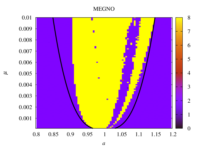
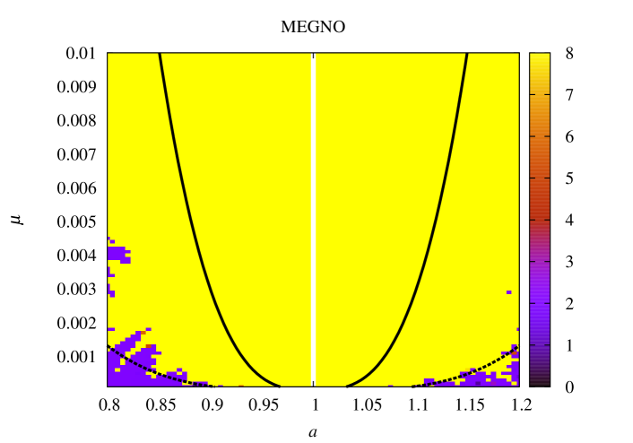
Figure 3: Stability boundary between regular (blue) and chaotic (yellow) regions for initially circular orbits: retrograde configuration (top panel) and prograde configuration (low panel). Black solid lines show edge of Hill’s region (width $(\mu/3)^{1/3}$) while black dashed lines show Wisdom’s stability boundary (width $1.33\,\mu^{2/7}$).

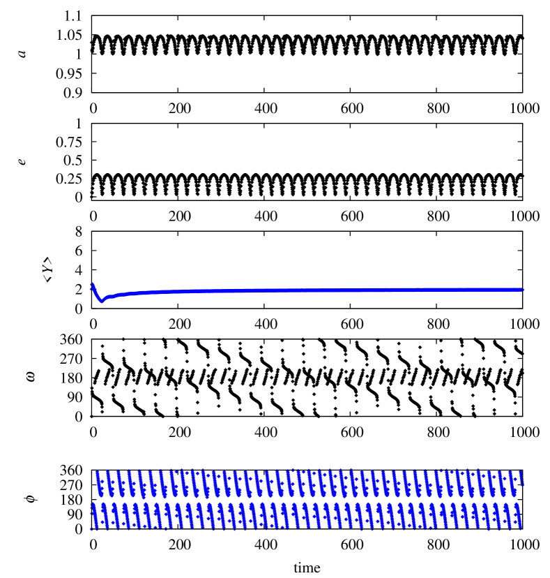
Figure 4: Orbit within stability island of Fig. 3 (top panel) for mass ratio $\mu=0.001$. From top to bottom: semi-major axis $a$, eccentricity $e$, mean MEGNO $<Y>$, argument of pericenter $\omega$, critical angle of 2D retrograde 1/1 resonance $\phi=\lambda-\lambda^{\prime}-2\,\omega$.

4 Stability maps of 2/1 and 1/2 retrograde resonances

As seen in Sect. 2.2 and Morais&Namouni2013CMDA the strongest retrograde resonance is the 1/1 (order 2), followed by the 2/1 and 1/2 (order 3). Here, we explore the stability of the 2/1 and 1/2 retrograde resonances, leaving a detailed study of the 1/1 retrograde resonance for a future publication. To that purpose we fix the mass ratio at $\mu=0.001$ (which represents a small body in the Sun-Jupiter system) and numerically integrate the equations of motion of the CR3BP, together with the variational equations and MEGNO equations Cincotta2000 ; Gozdziewski2003A&A for $5\,\times 10^{4}$ binary’s periods. As before, we set the maximum mean MEGNO $<Y>$ value for chaotic orbits as $8$ in order to have a high contrast between the regular (blue) and chaotic (yellow) regions.

4.1 The 2/1 retrograde resonance

The test particle’s initial conditions for the 2/1 retrograde resonance are: inclination $I=180^{\circ}$, semi-major axis in $(0.63-0.3\,R_{H},0.63+0.3\,R_{H})$ varying at steps $0.01\,R_{H}$, eccentricity in $(0,1)$ varying at steps $0.05$, $\Omega=\omega=0$, $\phi_{21}^{\star}=\lambda^{\star}-2\,\lambda^{\prime}-3\,\varpi^{\star}=0,180^{\circ}$, with $\lambda^{\star}=\lambda-2\,\Omega$, $\varpi^{\star}=\omega-\Omega$. In Fig. 5 we show the MEGNO maps for configurations with $\phi_{21}^{\star}=0$ (top panel) and $\phi_{21}^{\star}=180^{\circ}$ (low panel). The initial $(a,e)$ corresponding to the orbits in Fig. 1 (left) are marked in Fig. 5 (top), while those corresponding to the orbits in Fig. 1 (right) are marked in Fig. 5 (low).

The 2/1 retrograde resonant mode with $\phi_{21}^{\star}$ librating around 0 has close approaches with the planet between pericentre and apocentre (Fig. 1, left) while the one with $\phi_{21}^{\star}$ librating around $180^{\circ}$ has closest approaches with the planet at apocentre (Fig. 1, right). Hence the apocentric collision line (black) limits the border of the resonance in Fig. 5 (low panel). Libration in the resonance with centre $\phi_{21}^{\star}=180^{\circ}$ is only possible above this collision line and the border is chaotic (yellow) except for a gap between $0.63<a<0.64$ connecting the regular resonant and non-resonant regions.

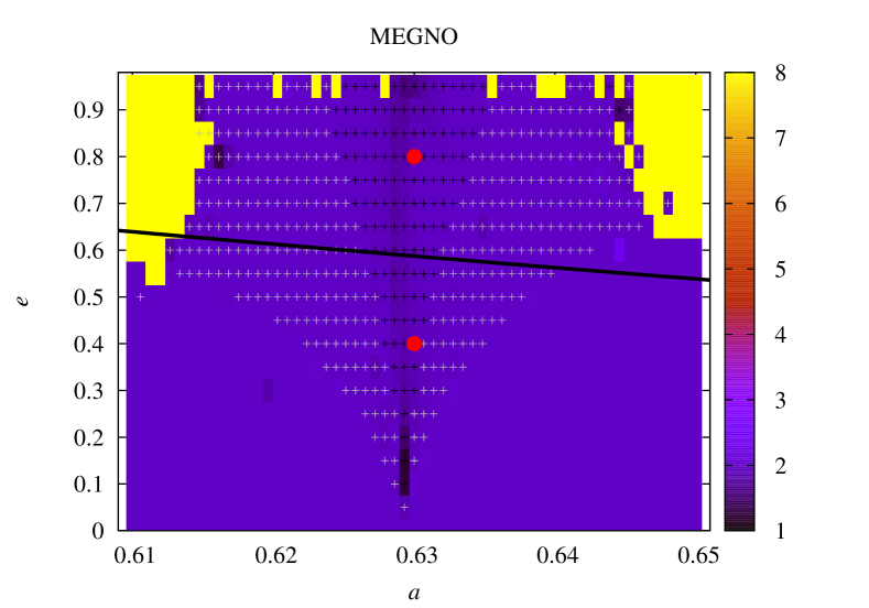
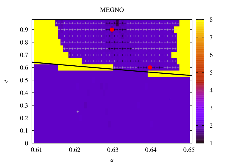
Figure 5: Stability map showing regular (blue) and chaotic (yellow) regions for retrograde 2/1 resonance with $\phi_{21}^{\star}=0$ (top) or $\phi_{21}^{\star}=180^{\circ}$ (low) when $\mu=0.001$. The symbol $+$ marks initial conditions such that $\phi_{21}^{\star}$ librates around 0 (top) or $180^{\circ}$ (low) with amplitude less than $50^{\circ}$ (black $+$), less than $300^{\circ}$ (gray $+$). The apocentric collision line is shown in black. The initial conditions corresponding to orbits in Fig. 1 (left) are marked with red circles on the top panel, while those corresponding to orbits in Fig. 1 (right) are marked with red circles on the low panel. The 2 gray $+$ symbols below the apocentric collision line (low panel) correspond to non-resonant orbits that are wrongly associated with large amplitude libration due to output sampling.

4.2 The 1/2 retrograde resonance

The test particle’s initial conditions for the 1/2 retrograde resonance are: inclination $I=180^{\circ}$, semi-major axis in $(1.59-0.3\,R_{H},1.59+0.3\,R_{H})$ varying at steps $0.01\,R_{H}$, eccentricity in $(0,1)$ varying at steps $0.05$, $\Omega=\omega=0$, $\phi_{12}^{\star}=2\,\lambda^{\star}-\lambda^{\prime}-3\,\varpi^{\star}=0,180^{\circ}$, with $\lambda^{\star}=\lambda-2\,\Omega$, $\varpi^{\star}=\omega-\Omega$. In Fig. 6 we show the MEGNO maps for configurations with $\phi_{12}^{\star}=0$ (top panel) and $\phi_{12}^{\star}=180^{\circ}$ (low panel). The initial $(a,e)$ corresponding to the orbits in Fig. 2 (left) are marked in Fig. 6 (top), while those corresponding to the orbits in Fig. 2 (right) are marked in Fig. 6 (low).

The 1/2 retrograde resonant mode with $\phi_{12}^{\star}$ librating around 0 has close approaches with the planet at pericentre (Fig. 2, left) while the one with $\phi_{12}^{\star}$ librating around $180^{\circ}$ has closest approaches with planet between apocentre and pericentre (Fig. 2, right). Hence the pericentric collision line (black) limits the border of the resonance in Fig. 6 (top panel). Libration in the resonance with centre $\phi_{12}^{\star}=0$ is only possible above this collision line which coincides with a chaotic (yellow) strip separating the regular resonant and non-resonant regions.

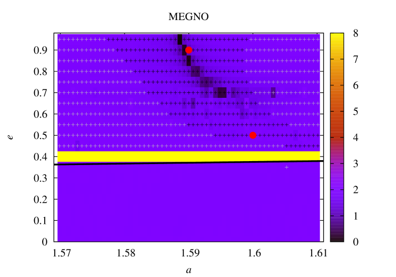
Figure 6: Stability map showing regular (blue) and chaotic (yellow) regions for retrograde 1/2 resonance with $\phi_{12}^{\star}=0$ (top) or $\phi_{12}^{\star}=180^{\circ}$ (low) when $\mu=0.001$. The symbol $+$ marks initial conditions such that $\phi_{12}^{\star}$ librates around 0 (top) or $180^{\circ}$ (low) with amplitude less than $50^{\circ}$ (black $+$), less than $300^{\circ}$ (gray $+$). The pericentric collision line is shown in black. The initial conditions corresponding to orbits in Fig. 2 (left) are marked with red circles on the top panel, while those corresponding to orbits in Fig. 2 (right) are marked with red circles on the low panel. The gray $+$ symbol just below the pericentric collision line (top panel) correspond to a non-resonant orbit that is wrongly associated with large amplitude libration due to output sampling.

5 Discussion

In this article we extended our work on the stability of retrograde configurations and the nature of retrograde resonance in the framework of the planar circular restricted three-body problem (CR3BP) consisting of a star, planet and test particle Morais&Giuppone2012MNRAS ; Morais&Namouni2013CMDA .

We obtained the stability boundary for retrograde configurations in the low mass (planetary) regime and showed that it is located within the planet’s Hill’s radius and that there is an asymmetry between the inner and outer boundaries. In contrast, the stability boundary for prograde configurations is located at several planet’s Hill’s radius and is approximated by Wisdom’s criterion of first order orbital resonances’ overlap. These results help understand the numerical simulations in Namouni&Morais2015MNRAS that showed that smooth migration capture in the 1/1 (coorbital) resonance occurs with probability 1 for planar retrograde configurations but with probability 0 for planar prograde configurations. We leave further investigation of this capture mechanism for a future publication

We obtained stability maps in a grid of semi-major axis versus eccentricity for the 2/1 and 1/2 retrograde resonances and showed the regions of libration of the critical arguments. The resonance borders are delimited by the collision separatrix with the planet whose location depends on the geometry of the resonance configuration and does not necessarily occur at pericentre (apocenter) for outer (inner) resonances. In the configurations where collision is possible at apocentre or pericentre our results agree with a study of prograde 3rd and 4th order resonances in the planar CR3BP by Erdi2012CMDA .

Stability studies of individual retrograde resonances are important in order to understand the origin of the Solar System small bodies in retrograde resonance with Jupiter and Saturn identified by Morais&Namouni2013MNRASL . Retrograde resonances may also exist in extrasolar systems Gayon&Bois2008 ; Gayon&Bois2009MNRAS ; Gozdziewski2013MNRAS although no cases have yet been confirmed due to the difficulty in measuring relative inclinations.

- (1) Cincotta, P.M., Simó, C.: Simple tools to study global dynamics in non-axisymmetric galactic potentials - I. A&AS147, 205–228 (2000). DOI 10.1051/aas:2000108
- (2) Eberle, J., Cuntz, M.: On the Reality of the Suggested Planet in the Octantis System. Astrophys. J. 721, L168–L171 (2010). DOI 10.1088/2041-8205/721/2/L168
- (3) Érdi, B., Rajnai, R., Sándor, Z., Forgács-Dajka, E.: Stability of higher order resonances in the restricted three-body problem. Celestial Mechanics and Dynamical Astronomy 113, 95–112 (2012). DOI 10.1007/s10569-012-9420-4
- (4) Gayon, J., Bois, E.: Are retrograde resonances possible in multi-planet systems? Astron. Astrophys. 482, 665–672 (2008). DOI 10.1051/0004-6361:20078460
- (5) Gayon-Markt, J., Bois, E.: On fitting planetary systems in counter-revolving configurations. Mon. Not. R. Astron. Soc. 399, L137–L140 (2009). DOI 10.1111/j.1745-3933.2009.00740.x
- (6) Goździewski, K.: Stability of the HD 12661 Planetary System. Astron. Astrophys. 398, 1151–1161 (2003). DOI 10.1051/0004-6361:20021713
- (7) Goździewski, K., Słonina, M., Migaszewski, C., Rozenkiewicz, A.: Testing a hypothesis of the Octantis planetary system. Mon. Not. R. Astron. Soc. 430, 533–545 (2013). DOI 10.1093/mnras/sts652
- (8) Morais, M.H.M., Correia, A.C.M.: Precession due to a close binary system: an alternative explanation for -Octantis? Mon. Not. R. Astron. Soc. 419, 3447–3456 (2012). DOI 10.1111/j.1365-2966.2011.19986.x
- (9) Morais, M.H.M., Giuppone, C.A.: Stability of prograde and retrograde planets in circular binary systems. Mon. Not. R. Astron. Soc. 424, 52–64 (2012). DOI 10.1111/j.1365-2966.2012.21151.x
- (10) Morais, M.H.M., Namouni, F.: Asteroids in retrograde resonance with Jupiter and Saturn. Mon. Not. R. Astron. Soc. 436, L30–L34 (2013). DOI 10.1093/mnrasl/slt106
- (11) Morais, M.H.M., Namouni, F.: Retrograde resonance in the planar three-body problem. Celestial Mechanics and Dynamical Astronomy 117, 405–421 (2013). DOI 10.1007/s10569-013-9519-2
- (12) Murray, C.D., Dermott, S.F.: Solar system dynamics. Cambridge University Press (1999)
- (13) Namouni, F., Morais, M.H.M.: Resonance capture at arbitrary inclination. Mon. Not. R. Astron. Soc. 446, 1998–2009 (2015). DOI 10.1093/mnras/stu2199
- (14) Perets, H.B., Kouwenhoven, M.B.N.: On the Origin of Planets at Very Wide Orbits from the Recapture of Free Floating Planets. Astrophys. J. 750, 83 (2012). DOI 10.1088/0004-637X/750/1/83
- (15) Ramm, D.J., Pourbaix, D., Hearnshaw, J.B., Komonjinda, S.: Spectroscopic orbits for K giants Reticuli and Octantis: what is causing a low-amplitude radial velocity resonant perturbation in Oct? Mon. Not. R. Astron. Soc. 394, 1695–1710 (2009). DOI 10.1111/j.1365-2966.2009.14459.x
- (16) Varvoglis, H., Sgardeli, V., Tsiganis, K.: Interaction of free-floating planets with a star-planet pair. Celestial Mechanics and Dynamical Astronomy 113, 387–402 (2012). DOI 10.1007/s10569-012-9429-8
- (17) Wisdom, J.: The resonance overlap criterion and the onset of stochastic behavior in the restricted three-body problem. Astron. J. 85, 1122–1133 (1980). DOI 10.1086/112778