Heavy Neutral Leptons – Advancing into the PeV domain

Abstract

Heavy neutral leptons (HNLs) are hypothetical particles able to explain neutrino oscillations and provide a mechanism for generating the baryon asymmetry of the Universe. Quantum corrections due to such particles give rise to flavor violating processes in the charged lepton sector. Based on the fact that these corrections grow with HNL masses, we improve existing constraints by orders of magnitude in mass and mixing angle. This allows us to probe part of the parameter space of leptogenesis with multi-TeV HNLs. We also show that one will be able to infer HNL parameters in a significant portion of the parameter space for TeV-PeV masses if charged lepton flavor violating signals are detected.

1 Introduction

Neutrinos in the Standard Model come in three different flavors. However, unlike other fermions, neutrinos change their flavor when propagating – a phenomenon known as neutrino oscillations (see e.g. (ParticleDataGroup:2020ssz, , Ch. 14)). The Standard Model forbids such a flavor-changing transition. Therefore neutrino oscillations imply the existence of extra quantum states, see e.g. deGouvea:2016qpx for an overview of neutrino mass models. One example of such states is given by right-chiral gauge singlet fermions, interacting with lepton doublets and the Higgs field via the Yukawa interactions. Being gauge singlets, these states can have Majorana masses, whose scale can be arbitrary Minkowski:1977sc ; Yanagida:1979as ; Glashow:1979nm ; Gell-Mann:1979vob ; Mohapatra:1979ia ; Mohapatra:1980yp ; Schechter:1980gr ; Schechter:1981cv . Compared to the Standard Model spectrum, this Type I seesaw model contains light neutrinos, $\nu_{i}$, $i=1,2,3$ whose masses and mixings fit the experimental neutrino measurements Esteban:2020cvm and, additionally, heavy neutral leptons (HNLs) $N_{I}$, $I=1,2\dots$ that interact similarly to neutrinos, but are much heavier and have a suppressed interaction strength due to the mixing angle $U_{\alpha}^{2}$. HNL masses can lie anywhere from $\mathcal{O}($1\text{\,}\mathrm{e}\mathrm{V}$)$ till $\mathcal{O}(${10}^{15}\text{\,}\mathrm{G}\mathrm{e}\mathrm{V}$)$, with experiments limiting their interaction from above (direct experimental searches, see Agrawal:2021dbo ; Abdullahi:2022jlv ) or from below (as in the case of primordial nucleosynthesis, see e.g. Sabti:2020yrt ; Boyarsky:2020dzc ; Bondarenko:2021cpc ).

HNLs can also be responsible for generating the matter-antimatter asymmetry of the Universe Fukugita:2002hu . This scenario (known as leptogenesis) has been actively developed since the 1980s (see, e.g., reviews Davidson:2008bu ; Pilaftsis:2009pk ; Shaposhnikov:2009zzb ; Buchmuller:2004nz ; Bodeker:2020ghk ). Different mechanism of low-scale leptogenesis have been suggested in Akhmedov:1998qx ; Asaka:2005pn ; Pilaftsis:2005rv . Recently, a unified description of these mechanisms in the case of two HNLS Klaric:2020phc ; Klaric:2021cpi and three HNLs Drewes:2021nqr has been presented. In both cases, the mixing angles $\Theta_{\alpha I}$ allowed by leptogenesis could be much larger than “naive” seesaw expectations. This can be realized in a technically natural way Wyler:1982dd ; Leung:1983ti ; Mohapatra:1986bd ; Branco:1988ex ; Gonzalez-Garcia:1988okv ; Shaposhnikov:2006nn ; Kersten:2007vk ; Abada:2007ux ; Gavela:2009cd ; Moffat:2017feq ; Drewes:2019byd if, for example, two HNLs form a pseudo-Dirac fermion Wolfenstein:1981kw ; Petcov:1982ya .

To mediate neutrino oscillations, HNLs should mix with neutrinos of several flavors. As a result, HNLs induce charged lepton flavor violating processes (cLFV) via tree-level (see e.g. Leung:1983ix, ; Gronau:1984ct, ; delAguila:2007qnc, ; Cvetic:2010rw, ; Cvetic:2012hd, ; Alva:2014gxa, ; Pascoli:2018heg, ; Fuks:2020att, ) or loop effects Petcov:1976ff ; Bilenky:1977du ; Marciano:1977wx ; Minkowski:1977sc ; Cheng:1980tp ; Lim:1981kv ; Langacker:1988up ; Pilaftsis:1992st ; Ilakovac:1994kj ; Illana:1999ww ; Illana:2000ic ; Pascoli:2003rq ; Pascoli:2003uh ; Arganda:2004bz ; Gorbunov:2014ypa ; Arganda:2016zvc ; Abada:2015oba ; Bolton:2022lrg ; Bai:2022sxq . Non-observations of cLFV processes constrain products $|U_{\alpha}U_{\beta\neq\alpha}|$. Assuming ratios between flavors, these constrains are the most powerful for $M_{N}\gtrsim\mathcal{O}($100\text{\,}\mathrm{G}\mathrm{e}\mathrm{V}$)$ not accessible via direct experimental searches (see e.g. deGouvea:2015euy, ; Fernandez-Martinez:2016lgt, ), see Bernstein:2013hba ; Calibbi:2017uvl for the recent experimental status of cLFV searches.

In this work, we highlight the non-trivial mass dependence of the cLFV processes and demonstrate that HNLs within the TeV-PeV mass range could significantly influence the magnitude and rates of cLFV events. More specifically, we show that for HNLs with masses $M_{N}\gg$1\text{\,}\mathrm{T}\mathrm{e}\mathrm{V}$$, the existing cLFV bounds are much stronger than previously estimated. In fact, they are one of the the strongest across the whole range of HNL masses.

This observation suggests the feasibility of using precision frontier measurements as a strategy for investigating the elusive high-mass domain of HNLs. We show that it is possible to explore a portion of the leptogenesis parameter space previously considered inaccessible. Furthermore, we demonstrate that potential observations of cLFV signals will allow for a more accurate determination of HNL parameters.

2 Basic definitions for heavy neutral leptons

In this section, we collect the basic definitions related to the Type-I Seesaw Lagrangian. While it contains only known results, they are needed for the consistency of our exposition.

2.1 Type I seesaw Lagrangian

The Lagrangian of the type-I seesaw model reads:

$$\mathcal{L}_{\mathrm{SM}+\mathrm{HNL}}=\mathcal{L}_{\mathrm{SM}}+i\bar{\nu}_{\mathrm{R}I}\not{\partial}\nu_{\mathrm{R}I}-F_{\alpha I}\bar{L}_{\alpha}\tilde{\Phi}\,\nu_{\mathrm{R}I}-\frac{1}{2}\bar{\nu}_{\mathrm{R}I}^{c}\,M_{I}\,\nu_{\mathrm{R}I}+\mathrm{h.c.}$$ (1)

where $\mathcal{L}_{\mathrm{SM}}$ is the SM Lagrangian, $\nu_{\mathrm{R}I}$, $I=1,\dots,\mathcal{N}$ are the right-chiral components of neutrino fields – SM gauge singlets –, $L_{\alpha}$ is SM lepton doublets, $\tilde{\Phi}=i\sigma_{2}\Phi$ where $\Phi$ is the Higgs doublet, $F_{\alpha I}$ is a Yukawa matrix, and $M_{I}$ is the Majorana masses of right-handed neutrinos. Finally, sum over $I$ and $\alpha$ is assumed in (1). After spontaneous symmetry breaking, the model will acquire Dirac masses, $(m_{D})_{\alpha I}$ mixing right and left-handed neutrino components. In the case $|m_{D}|\ll M_{I}$, the diagonalization of the mass matrix results in three fields $\nu_{i}$ with light masses, $m_{i}$ and $\mathcal{N}$ heavy fields $N_{I}$ with heavy masses $M_{I}$ of the shape:

$$(m_{\nu})_{\alpha\beta}\simeq-\sum_{I}(m_{D})_{\alpha I}\frac{1}{M_{I}}(m_{D})_{I\beta},$$ (2)

where

$$(m_{\nu})_{\alpha\beta}=\sum_{i=1}^{3}V^{\text{\sc pmns}}_{\alpha i}m_{i}V^{\text{\sc pmns}}_{i\beta}\,,$$ (3)

$V^{\text{\sc pmns}}$ is the PMNS matrix Petcov:2013poa , and $\alpha=e,\mu,\tau$. Eq. (2) is the famous seesaw mechanism Minkowski:1977sc ; Yanagida:1979as ; Mohapatra:1979ia ; Mohapatra:1980yp ; Schechter:1980gr ; Schechter:1981cv .

After diagonalization, neutrinos in the flavor basis are in a superposition of light and heavy mass states:

$$\nu_{\alpha}=V^{\text{\sc pmns}}_{\alpha i}\,\nu_{i}+\Theta_{\alpha I}\,N_{I}^{c}\,=\mathcal{U}_{\alpha i}\,n_{i}+\mathcal{U}_{\alpha I}\,n_{I}\,,$$ (4)

where $\Theta$ is the left-right neutrino mixing angle, and the $3\times(3+\mathcal{N})$ matrix $\mathcal{U}$ is defined as

$$\mathcal{U}\equiv\left(V^{\text{\sc pmns}},\Theta\right)$$ (5)

Eq. (4) makes it clear that HNLs will interact in the exact same way as active neutrinos do, with the notable exception that it will be suppressed by the mixing angle $\Theta_{\alpha I}$ forming a $3\times\mathcal{N}$ matrix with components

$$\Theta_{\alpha I}=\frac{(m_{D})_{\alpha I}}{M_{I}}\,.$$ (6)

Furthermore, we can define flavor mixing angles

$$U_{\alpha}^{2}\equiv\sum_{I}|\Theta_{\alpha I}|^{2}\,,$$ (7)

to which in the case of nearly degenerate HNLs the signal would be proportional.

In addition, after diagonalization interactions between neutral leptons and SM gauge bosons get modified from the usual SM ones. These interactions read as:

$$\mathcal{L}_{W} =\frac{g}{\sqrt{2}}\,\mathcal{U}_{\alpha i}\,\bar{\ell}_{\alpha}\,\not{W}^{-}\,P_{L}\,n_{i}+\text{h.c.}\,,$$ (8)

$$\mathcal{L}_{Z} =\frac{g}{2c_{w}}\bar{n}_{i}\not{Z}\left[\mathcal{C}_{ij}^{\phantom{\ast}}P_{L}-\mathcal{C}_{ij}^{\ast}P_{R}\right]n_{j}\,,$$ (9)

$$\mathcal{L}_{\phi^{\pm}} =\frac{g}{\sqrt{2}m_{w}}\mathcal{U}_{\alpha i}\,\phi^{-}\left[\bar{\ell}_{\alpha}\left(m_{i}P_{R}-m_{\alpha}P_{L}\right)n_{i}\right]+\text{h.c.}\,,$$ (10)

$$\mathcal{L}_{\phi^{0}} =\frac{ig}{4m_{w}}\,\phi^{0}\,\bar{n}_{i}\left[\mathcal{C}^{\phantom{\ast}}_{ij}\left(m_{j}\,P_{R}-m_{i}\,P_{L}\right)+\mathcal{C}_{ij}^{\ast}\left(m_{i}P_{R}-m_{j}P_{L}\right)\right]n_{j}\,,$$ (11)

$$\mathcal{L}_{h} =-\frac{g}{4m_{w}}\,h\,\bar{n}_{i}\left[\mathcal{C}^{\phantom{\ast}}_{ij}\left(m_{j}\,P_{R}+m_{i}\,P_{L}\right)+\mathcal{C}_{ij}^{\ast}\left(m_{i}P_{R}+m_{j}P_{L}\right)\right]n_{j}\,,$$ (12)

where $\mathcal{C}_{ij}=\sum_{\alpha}\mathcal{U}_{\alpha i}^{\ast}\,\mathcal{U}_{\alpha j}^{\phantom{\ast}}$. We properly used the Feynman rules regarding Majorana particles Denner:1992vza , especially with regards to vertices involving lepton number violating (LNV) processes or in interactions with neutral bosons that involve two Majorana particles.

There is a number of relations that the $\mathcal{U},\mathcal{C}$ and mass matrix of neutral fermions follow that can be found in Appendix A.

2.2 Parametrization of the mixing angles

A matrix $\Theta$ that automatically satisfies the seesaw relation (2) is given by the Casas-Ibarra parametrization Casas:2001sr :

$$\Theta=i\,V^{\text{\sc pmns}}\sqrt{m_{\nu}}\,R\,\frac{1}{\sqrt{M_{N}}},$$ (13)

where $m_{\nu}=\mathop{\mathrm{diag}}(m_{1},m_{2},m_{3})$, $M_{N}=\mathop{\mathrm{diag}}(M_{1},\dots,M_{\mathcal{N}})$ and the $3\times\mathcal{N}$ matrix $R$ obeys the relation: $R^{T}R=\mathbbm{1}$.

The model has introduced a total of new $7\mathcal{N}-3$ different parameters to the SM. Neutrino oscillation data already constraints some of them: two different mass splittings and three mixing angles from the PMNS matrix Esteban:2020cvm . In the active neutrino sector, we additionally have the lightest neutrino mass, two Majorana CP phases, $\delta_{\mathrm{CP}}$, one Dirac CP phase, and the discrete choice of mass hierarchy.

Throughout this work, we are dealing with the simplest realistic case of $\mathcal{N}=2$. In this case, the lightest neutrino mass is set automatically to zero, and only a linear combination of two Majorana phases contributes, which we will call $\eta$. This leaves us with three unknown parameters in the active neutrino sector, with the already mentioned unbeknownst mass hierarchy. In this model, the $R$ matrix depends on the choice of hierarchy Ibarra:2003up ; Petcov:2005jh :

$$R^{\mathrm{NO}}=\begin{pmatrix}0&0\\ \cos\omega&\sin\omega\\ -\sin\omega&\cos\omega\end{pmatrix},\hskip 28.45274ptR^{\mathrm{IO}}=\begin{pmatrix}\cos\omega&\sin\omega\\ -\sin\omega&\cos\omega\\ 0&0\end{pmatrix},\qquad\omega\in\mathbbm{C}\,.$$ (14)

It is useful to define the sum of the absolute value squared of all the elements of $|\Theta_{\alpha I}|^{2}$, $U_{\mathrm{tot}}^{2}$, in terms of Casas-Ibarra parameters, and HNL and active neutrino masses. The expression becomes simple when considering two HNLs with equal masses:

$$U_{\mathrm{tot}}^{2}=\sum_{\alpha I}\left|\Theta_{\alpha I}\right|^{2}=\frac{\sum_{i}m_{i}}{M}\,\cosh(2\mathop{\mathrm{Im}}{\omega})\,,$$ (15)

the reader may find a more general expression in Eijima:2018qke for non-degenerate HNL masses.

3 Decoupling behaviour

cLFV observables receive contributions from HNLs, appearing in the loop once or twice: compare the diagram (a) with the diagrams (b) and (c) in Figure 1 (see Appendix B for details). Two-HNL contributions bear similarity with the “penguin diagrams” in flavor physics (see e.g., Shifman:1995hc, ) and appear whenever $Z$ or Higgs bosons contribute to the diagrams. Schematically, the conversion rate $\mu\to e$ on a nucleus (the process that will give the strongest bounds) has the form

$$\mathop{\mathrm{CR}}\nolimits(\mu\to e)\propto\Lambda_{e\mu}U_{\mathrm{tot}}^{4}\Bigl{|}c_{0}(M_{N})+U_{\mathrm{tot}}^{2}c_{2}(M_{N})\Bigr{|}^{2}$$ (16)

where $U_{\mathrm{tot}}^{2}=\sum_{\alpha,I}\bigl{|}\Theta_{\alpha I}\bigr{|}^{2}$ and

$$\Lambda_{\alpha\beta}\equiv\frac{\left|\sum_{I}\Theta_{\alpha I}\Theta_{\beta I}^{*}\right|^{2}}{U_{\mathrm{tot}}^{4}}$$ (17)

The functions $c_{i}(M_{N})$ scale for HNL mass $M_{N}\gg m_{W}$ as:

$$c_{2}(M_{N})\propto\frac{M_{N}^{2}}{m_{W}^{2}}\gg c_{0}(M_{N})\propto\log\left(\frac{M_{N}}{m_{W}}\right)$$ (18)

As a result, although subdominant due to $U_{\mathrm{tot}}^{2}\ll 1$, the strong mass dependence of $c_{2}(M_{N})$ makes the second term larger than the first one. As a result, HNL contributions to cLFV processes become much stronger at large masses than previously estimated.

The above result seemingly contradicts the “Decoupling Theorem” Appelquist:1974tg , as loop effects of heavy particles grow with mass. However, theories that undergo spontaneous symmetry breaking violate this theorem if dimensionless couplings – in our case, the Yukawa coupling that determines the Dirac mass — are sent to infinity (see e.g. Collins:1978wz ; Cheng:1991dy ; Tommasini:1995ii ; DHoker:1984mif ; DHoker:1984izu , or the book (Collins:1984xc, , Chapter 8)). At a technical level, this happens because the coupling between HNLs and Goldstone bosons is proportional to the Yukawa couplings, and in turn, to the Dirac Mass term $m_{D}\sim\Theta M_{N}$ (see Eq. 6). If one considers $\Theta$ and $M_{N}$ as independent parameters, then Dirac mass term grows as $M_{N}\to\infty$, and there is no decoupling. On the other hand, keeping Yukawa constants fixed implies $|\Theta|\propto M_{N}^{-1}$. As a result, the effect (16) disappears.

By increasing $M_{N}$ at fixed $|\Theta|$ the HNL decay width $\Gamma_{N}\propto|\Theta|^{2}M_{N}^{3}$ exceeds $\frac{1}{2}M_{N}$ (equivalently, Yukawa coupling constant of neutrino exceeds $\sqrt{4\pi}$). The corresponding non-perturbative region is shaded in gray below. See Chanowitz:1978mv ; Durand:1989zs ; Fajfer:1998px ; Ipek:2018sai , and Appendix D for a brief discussion on the stability on second-order terms.

Indeed, the non-decoupling behaviour of HNLs implies that when we match the amplitudes to a series of EFT operators, we will find that such operators will depend on HNL masses or on their Yukawa couplings, and this is exactly what happens when one does a one-loop matching to different EFT operators Zhang:2021jdf .

Figure 1: One-loop diagrams contributing to the $\mu\to e$ conversion process, including 2 HNL “penguin” diagrams (a). Diagrams containing HNLs that dress external lines are not shown (see Appendix C for the full list of such diagrams).

Figure 2: Improved experimental limits on HNLs coupling from charged lepton flavor violation processes (solid lines) for the normal ordering (left) and inverted ordering (right). The strongest bound comes from the $\mu\to e$ conversion in gold SINDRUMII:2006dvw . Blue shaded region: previous constraints, not including cLFV. Gray shaded region: non-perturbative regime (see text for details). Dotted lines: previous cLFV constrains from the works Alonso:2012ji ; deGouvea:2015euy ; Abada:2015oba ; Fernandez-Martinez:2016lgt ; Abada:2018nio . Results are expressed in terms of $U_{\mathrm{tot}}^{2}$ for flavor ratios (19), see text for details.

4 Results

Using the proper expression for the cLFV branching ratios/conversion rates, we reinterpret the existing limits on HNL parameters as shown in Figure 2 (solid lines). To efficiently present and compare our results, we fix ratios of $U_{\alpha}^{2}$ to the benchmark values, dictated by neutrino oscillations Agrawal:2021dbo :

$$U_{e}^{2}:U_{\mu}^{2}:U_{\tau}^{2}=\left\{\begin{array}[]{ll}0.06:0.48:0.46&\text{(NO)}\\ 0.33:0.33:0.33&\text{(IO)}\end{array}\right.$$ (19)

(see Tastet:2021vwp ) and express all the limits in terms of the total mixing angle, $U_{\mathrm{tot}}^{2}$. Compared to the electroweak precision data constraints Fernandez-Martinez:2016lgt , our bounds improve by as much as three orders of magnitude. Compared to the previous cLFV constrains (not taking into account the $c_{2}(M_{N})$ terms), we improve the bounds by roughly one order of magnitude for masses $\mathcal{O}($100\text{\,}\mathrm{T}\mathrm{e}\mathrm{V}$)$. To the best of our knowledge, the constraints from $\mu\to e$ conversion in gold SINDRUMII:2006dvw have not been previously used to derive bounds on HNL parameters in the multi-TeV region, and the only work that took into account $c_{2}(M_{N})$ terms when deriving the cLFV limits was deGouvea:2015euy that however did not explore them beyond $\sim$10\text{\,}\mathrm{T}\mathrm{e}\mathrm{V}$$.

The maximal mass, probed by these cLFV processes, for degenerate HNLs, is extended from $\sim${10}^{5}\text{\,}\mathrm{G}\mathrm{e}\mathrm{V}$$ to about ${10}^{6}\text{\,}\mathrm{G}\mathrm{e}\mathrm{V}$. Our limits are stronger than LHC searches in the range $M_{N}\gtrsim$20\text{\,}\mathrm{G}\mathrm{e}\mathrm{V}$$ CMS:2018iaf ; ATLAS:2019kpx ; CMS:2022fut ; ATLAS:2022atq . Future cLFV experiments Mihara:2013zna may probe HNLs up to incredible masses of $M_{N}\sim$3\text{\times}{10}^{7}\text{\,}\mathrm{G}\mathrm{e}\mathrm{V}$$ (i.e. $30\text{\,}\mathrm{P}\mathrm{e}\mathrm{V}$). Our results get more pronounced as Yukawa couplings grow.

The constraints from $\mu\to 3e$ and muon conversion in the case of HNLs with a hierarchical mass spectrum are presented Appendix B.

Figure 3: Constrains on HNL parameters from future cLFV experiments for the normal Ordering (left) and inverted Ordering (right). Two HNL contributions are taken into account where applicable. Notice the different range of y-axes as compared to Figure 2. Maximal probed mass may reach $3\text{\times}{10}^{7}\text{\,}\mathrm{G}\mathrm{e}\mathrm{V}$ should the recently proposed $\mu\to e$ conversion experiment CGroup:2022tli be performed. Results are expressed in terms of $U_{\mathrm{tot}}^{2}$ for flavor ratios (19), see text for details. The black line in the right plot is the upper boundary of the parameter space where successful leptogenesis with 3 HNLs is possible Drewes:2021nqr (dashed-dotted part is an extrapolation to guide the eye). The sensitivity reach of several future experiments (SHiP SHiP:2018xqw , FCC-ee Blondel:2014bra , FCC-hh Pascoli:2018heg ) is shown as thin dashed lines.

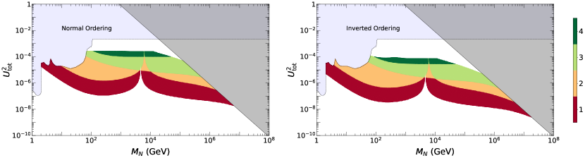
Figure 4: Parameter space probed by future cLFV experiments for the normal ordering (left) and inverted ordering (right). Color bands illustrate where one or several future cLFV experiments have sensitivity and thus can observe a signal. Observation of a signal in two or more experiments (orange to green bands) will allow for reconstructing parameters of realistic HNL models. The white region is explored by the current cLFV experiments.

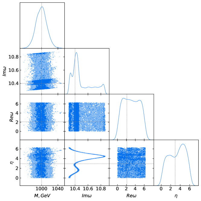
Figure 5: Reconstruction of HNL parameters in case of two cLFV detections. HNL parameters, explaining neutrino data Esteban:2020cvm , assuming normal ordering, and that the provided cLFV signals are within the future discovery zone (c.f. Figure 4). We built a likelihood function, depending on four parameters (shown in the plots as straight lines) and explored it with MCMC sampling. $\omega$ is the mixing angle from the Casas-Ibarra matrix and $\eta$ is the Majorana Phase (see Sec. 2.2). Dotted grey lines show the “true” parameters.

5 Indirect detection of TeV–PeV HNLs

In the wide range of HNL parameters, two or more future cLFV experiments can detect a signal, as Figure 4 demonstrates. Non-trivial mass dependences of $\mu\to e$ conversion rates and $\mu\to 3e$ processes open a possibility to recover HNL parameters in this case. Similar idea has been explored in the past, (see e.g. Chu:2011jg, ; Alonso:2012ji, ; Hambye:2013jsa, ), albeit without “penguin” contributions that change the mass dependence.

Consider the simplest HNL model explaining neutrino oscillation data – two HNLs with almost degenerate masses. The cLFV branching ratios (16) depend in this case on three parameters: common mass, $M_{N}$, total mixing angle, $U_{\mathrm{tot}}^{2}$, and $\Lambda_{e\mu}$. While flavor mixing angles, $U_{\alpha}^{2}$ can still vary in the wide range, $\Lambda_{e\mu}$ changes only weakly if the mass ordering and the CP phase is known (see e.g. Patterson:2015xja, ; DUNE:2021mtg, ). As a result, given two cLFV measurements ($\mu\to e$ conversions and $\mu\to 3e$ measurement, Table 1), the HNL parameters can be reconstructed.

To demonstrate the feasibility of parameter reconstruction, we have randomly assumed HNL parameters in the light green region of Figure 4 and computed the rates of the cLFV processes. Assuming that these were the measured rates (with 50% measurement error), we defined the log-likelihood as a mean square deviation between the predicted and “measured” rates. We performed an MCMC scan of the parameter space using the emcee pacakge Foreman-Mackey:2012any . Using Kernel Density Estimation method implemented in GetDist Lewis:2019xzd , we successfully recovered both mass and the total mixing angle, see Figure 5.

Process	Current bounds	Future limits
Processes, proportional to $\Lambda_{e\mu}$
$\mu\to e\gamma$	$4.2\times 10^{-13}$ MEG:2016leq	$6\times 10^{-14}$ MEGII:2018kmf
$\mu\to 3e$	$1.0\times 10^{-12}$ SINDRUM:1987nra	$1\times 10^{-16}$ Blondel:2013ia ; Berger:2014vba
$\mu\to e$	$4.6\times 10^{-11}$ (Pb) SINDRUMII:1993gxf	$1\times 10^{-17}$ (Al) Mu2e:2014fns ; COMET:2018auw
conversion	$4.3\times 10^{-12}$ (Ti) SINDRUMII:1996fti	$1\times 10^{-19}$ (Ti) CGroup:2022tli
	$7.0\times 10^{-13}$ (Au) SINDRUMII:2006dvw
$Z\to e\mu$	$7.5\times 10^{-7}$ ATLAS:2014vur	$1\times 10^{-10}$ Dam:2018rfz
$h\to e\mu$	$6.1\times 10^{-5}$ ATLAS:2019old
Processes, proportional to $\Lambda_{e\tau}$
$\tau\to e\gamma$	$3.3\times 10^{-8}$ BaBar:2009hkt	$3\times 10^{-9}$ Belle-II:2018jsg
$\tau\to 3e$	$2.7\times 10^{-8}$ Hayasaka:2010np	$5\times 10^{-10}$ Belle-II:2018jsg
$Z\to e\tau$	$9.8\times 10^{-6}$ OPAL:1995grn	$1\times 10^{-9}$ Dam:2018rfz
$h\to e\tau$	$4.7\times 10^{-3}$ ATLAS:2019pmk
Processes, proportional to $\Lambda_{\mu\tau}$
$\tau\to\mu\gamma$	$4.4\times 10^{-8}$ BaBar:2009hkt	$1\times 10^{-9}$ Belle-II:2018jsg
$\tau\to 3\mu$	$2.1\times 10^{-8}$ Hayasaka:2010np	$5\times 10^{-10}$ Belle-II:2018jsg
$Z\to\tau\mu$	$1.2\times 10^{-5}$ DELPHI:1996iox	$1\times 10^{-9}$ Dam:2018rfz
$h\to\tau\mu$	$2.5\times 10^{-3}$ CMS:2017con

Table 1: Present cLFV limits and future projections for various $\Lambda_{\alpha\beta}$ processes.

6 Discussion

Heavy neutral leptons couple to neutrinos of different flavors and thus give rise to charged lepton flavor violating processes. Many laboratories worldwide (Table 1) pursue searches for these cLFV processes. Their negative results provide constraints on HNL parameters, see e.g. Fernandez-Martinez:2016lgt . For $\mu\to e$ conversion rate, the HNL contributions to cLFV processes contain terms proportional to the $U_{\mathrm{tot}}^{4}$ and those, proportional to the $U_{\mathrm{tot}}^{8}$ (with the common factor $\Lambda_{e\mu}$, Eq. (17)). The latter terms have been neglected in the past. However, for $M_{N}\gg m_{W}$, the term $U_{\mathrm{tot}}^{8}$ is multiplied by the growing function in mass, $(M_{N}/m_{W})^{4}$. Therefore, for $M_{N}\gg m_{W}$ this second term becomes dominant, making constraints stronger by orders of magnitude, as we showed in this work (see Figure 2 for current and Figure 3 for future sensitivity). The resulting constraints for realistic HNL models (i.e. those where HNLs mediate neutrino oscillations) allow us to reach limits on the mixing angle compared to the best direct searches for masses up to $\sim$30\text{\,}\mathrm{P}\mathrm{e}\mathrm{V}$$. In particular, these constraints exceed by orders of magnitude in mass reach and coupling sensitivity those that can be achieved with direct searches for HNLs at FCC-hh Alva:2014gxa ; Pascoli:2018heg ; Fuks:2020att ; Abdullahi:2022jlv .

We derived our main results for the case of the 2 HNL model, but they are readily generalizable to the models with 3 HNLs (see Appendix B). In this case, cLFV measurements can probe part of the parameter space of the leptogenesis Drewes:2021nqr as Figure 3 demonstrates. See also Granelli:2022eru .

The present analysis has assumed benchmark flavor ratios (19). Scanning over the whole allowed range of $\Lambda_{\alpha\beta}$ does not qualitatively change our results (see also Abada:2021zcm ). In particular, in models with 2 HNLs, even in the case of normal ordering, where $U_{e}^{2}\ll U_{\mu,\tau}^{2}$, the processes involving LFV in the $e\mu$ sector dominate the current and future limits. In the models with 3 HNLs the suppression of the electron mixing may become even more extreme Abdullahi:2022jlv , potentially making $\mu\tau$ channels competitive. This demonstrates importance of the future searches, such as TauFV Alekhin:2015byh ; Beacham:2019nyx ; EuropeanStrategyforParticlePhysicsPreparatoryGroup:2019qin at the CERN Beam Dump Facility Ahdida:2019ubf measurement $\tau\to 3\mu$ processes at the level $\sim 10^{-10}$.

Appendix A Unitarity and Seesaw relations

The matrix elements $\mathcal{U}_{\alpha i}$ of the matrix $\mathcal{U}$, defined by Eq. (5), obey the following unitarity and seesaw relations Pilaftsis:1992st :

$$\sum_{i=1}^{3+\mathcal{N}}\mathcal{U}_{\alpha i}^{\phantom{\ast}}\,\mathcal{U}_{\beta i}^{\ast}=\delta_{\alpha\beta}\,,$$ (20)

$$\sum_{\alpha=e,\mu,\tau}\mathcal{U}_{\alpha i}^{\phantom{\ast}}\,\mathcal{U}_{\alpha j}^{\ast}=\mathcal{C}_{ij}\,,$$ (21)

$$\sum_{i=1}^{3+\mathcal{N}}\mathcal{U}_{\alpha i}^{\phantom{\ast}}\,\mathcal{C}_{ij}^{\phantom{\ast}}=\mathcal{U}_{\alpha i}\,,\hskip 28.45274pt\sum_{i=1}^{3+\mathcal{N}}\mathcal{C}_{ij}^{\phantom{\ast}}\,\mathcal{C}_{ik}^{\ast}=\mathcal{C}_{kj}\,,$$ (22)

$$\sum_{i=1}^{3+\mathcal{N}}\mathcal{U}_{\alpha i}^{\phantom{\ast}}\,\mathcal{U}_{\beta i}^{\phantom{\ast}}\,m_{i}=\sum_{i=1}^{3+\mathcal{N}}\mathcal{U}_{\alpha i}^{\phantom{\ast}}\,\mathcal{C}_{ij}^{\ast}\,m_{i}=\sum_{i=1}^{3+\mathcal{N}}\mathcal{C}_{ij}^{\phantom{\ast}}\,\mathcal{C}_{ik}^{\phantom{\ast}}\,m_{i}=0\,.$$ (23)

Relation (20) is the unitarity of the $\mathcal{U}$ matrix, whereas (21) defines the coupling between the $Z$ boson and $n_{i}n_{j}$. The equalities (22) are a consequence of two previous ones, and the last set of equivalences are nothing but the Seesaw relation, expressed in Eq. (2), but written in terms of $\mathcal{U}$ and $\mathcal{C}$.

Appendix B Phenomenology of cLFV processes

B.1 Relevant branching ratios and rates

We present all the pertinent diagrams in Appendix C. We calculated the corresponding amplitudes using the Mathematica packages: FeynCalc Shtabovenko:2020gxv , FeynArts Hahn:2000kx and Package-X Patel:2016fam and cross-checked the results against existing literature Minkowski:1977sc ; Marciano:1977wx ; Lim:1981kv ; Riazuddin:1981hz ; Langacker:1988up ; Cheng:1980tp ; Ilakovac:1994kj ; Chang:1994hz ; Pilaftsis:1998pd ; Ioannisian:1999cw ; Deppisch:2005zm ; Pilaftsis:2005rv ; Deppisch:2010fr ; Alonso:2012ji . To include the “HNL penguin” diagrams, we modified the FeynRules model file HeavyN Alva:2014gxa ; Degrande:2016aje ; Pascoli:2018heg and nloFRModel and added previously missing vertices involving the coupling between two HNLs and neutral bosons – those in Eq. (9), (11) and (10). The updated model is available at repo .

The diagrams that display the apropos asymptotic behavior in mass are shown below in Appendix C in green. The anomalous $Z\ell_{\alpha}\ell_{\beta}$ coupling shown in Fig. (C.8) also gives a non-decoupling effect on both $\ell_{\beta}\to 3\ell_{\alpha}$ and muon conversion in a nucleus processes.

The amplitude of diagram (j) in Fig. (C.8) contains two different parts, one dependent on $\mathcal{C}^{\phantom{\ast}}_{ij}$ and another on $\mathcal{C}^{\ast}_{ij}$, the latter is suppressed in the case of degenerate HNLs (see B.3). Both parts are asymptotic in mass, the two of them get two powers in mass from the couplings between HNLs and Goldstone bosons. The former also gets two additional powers in mass coming from the propagators of the HNLs, which cancels the mass suppression coming from the loop functions. The latter gets the momentum from the HNL propagators, but the leading terms of the loop functions are not suppressed in mass. Overall, both amplitudes will have a mass squared dependence.

The origin of the asymptotic behavior of diagrams (e) and (i) in Fig. (C.9) can be explain similarly. Both diagrams get four powers in mass from the couplings between the HNLs and Goldstone bosons. Diagram (e) picks up the momentum terms from the propagators of the HNLs, this gives it a loop function which removes two powers of mass from the amplitude. Whereas, diagram (i) picks up the mass terms from the propagators, but has a stronger suppression from the loop functions. All in all, both terms will have a mass squared dependence.

The diagrams that have a red letter attached to them are divergent. All of these divergences vanish when we sum up the diagrams. Namely, diagrams (c, d, e) in Figures C.7–C.8 have their divergences vanish due to the unitarity relation expressed in Eq. (20), this is also the case for Diagram (i) in Fig. C.8. Whereas for Diagram (j) in Fig. (C.8 vanishes due to the Seesaw relation, expressed in Eq. (23).

Diagrams (f, g, h) in both, Figure C.7 and Figure C.8 vanish when the three diagrams are summed. It should also be noted that in the limit when the four-momentum squared of the outer boson is zero, $Q^{2}\to 0$, the sum of the three diagrams vanishes completely. The reason for this becomes clear when the calculation is done in the $R_{\xi}$ gauge, where the three diagrams are completely gauge-dependent.

B.2 Branching ratio for cLFV processes

The cLFV processes that receive contributions from “HNL penguins” or “HNL box diagrams” include $\ell_{\beta}\to\ell_{\alpha}\ell_{\gamma}\bar{\ell}_{\eta}$. The formulas of the branching ratios are different depending on whether $\alpha=\gamma=\eta,\alpha=\eta\neq\gamma$, or $\alpha=\gamma\neq\eta$. In the first case, there is an additional factor coming from identical fermions in the final state that is not found in the second case; and in the third case, only box diagrams contribute, $Z$ and $\gamma$ penguins do not contribute at 1-loop.

The formulas of the branching ratios for these decays are:

$$\mathrm{BR}(\ell_{\beta}\to 3\ell_{\alpha})= \frac{\alpha_{w}^{4}}{24576\,\pi^{3}}\,\frac{m_{\beta}^{4}}{M_{W}^{4}}\,\frac{m_{\beta}}{\Gamma_{\beta}}\left\{2\left|\frac{1}{2}F_{\text{box}}^{\beta 3\alpha}+F_{Z}^{\beta\alpha}-2s_{w}^{2}\,(F_{Z}^{\beta\alpha}-F_{\gamma}^{\beta\alpha})\right|^{2}\right.$$

$$+ \left.4s_{w}^{4}\,|F_{Z}^{\beta\alpha}-F_{\gamma}^{\beta\alpha}|^{2}+16s_{w}^{2}\,\mathrm{Re}\left[(F_{Z}^{\beta\alpha}+\frac{1}{2}F_{\text{box}}^{\beta 3\alpha})\,G_{\gamma}^{\beta\alpha\ast}\right]\right.$$

$$- \left.48s_{w}^{4}\,\mathrm{Re}\left[(F_{Z}^{\beta\alpha}-F_{\gamma}^{\beta\alpha})\,G_{\gamma}^{\beta\alpha\ast}\right]+32s_{w}^{4}\,|G_{\gamma}^{\beta\alpha}|^{2}\left[\log\frac{m_{\beta}^{2}}{m_{\alpha}^{2}}-\frac{11}{4}\right]\right\}\,,$$ (24)

$$\mathrm{BR}(\ell_{\beta}\to\ell_{\alpha}\bar{\ell}_{\alpha}\ell_{\gamma})= \frac{\alpha_{w}^{4}}{24576\,\pi^{3}}\,\frac{m_{\beta}^{4}}{M_{W}^{4}}\,\frac{m_{\beta}}{\Gamma_{\beta}}\left\{\left|F_{\text{box}}^{\beta\gamma\alpha\alpha}+F_{Z}^{\beta\alpha}-2s_{w}^{2}\,(F_{Z}^{\beta\alpha}-F_{\gamma}^{\beta\alpha})\right|^{2}\right.$$

$$+ \left.4s_{w}^{4}\,|F_{Z}^{\beta\alpha}-F_{\gamma}^{\beta\alpha}|^{2}+8s_{w}^{2}\,\mathrm{Re}\left[(F_{Z}^{\beta\alpha}+F_{\text{box}}^{\beta\gamma\alpha\alpha})\,G_{\gamma}^{\beta\alpha\ast}\right]\right.$$

$$- \left.32s_{w}^{4}\,\mathrm{Re}\left[(F_{Z}^{\beta\alpha}-F_{\gamma}^{\beta\alpha})\,G_{\gamma}^{\beta\alpha\ast}\right]+32s_{w}^{4}\,|G_{\gamma}^{\beta\alpha}|^{2}\left[\log\frac{m_{\beta}^{2}}{m_{\alpha}^{2}}-3\right]\right\}\,,$$ (25)

$$\mathrm{BR}(\ell_{\beta}\to\ell_{\alpha}\ell_{\alpha}\bar{\ell}_{\gamma})= \frac{\alpha_{w}^{4}}{49152\,\pi^{3}}\,\frac{m_{\beta}^{4}}{M_{W}^{4}}\,\frac{m_{\beta}}{\Gamma_{\beta}}\left|F_{\text{box}}^{\beta\alpha\alpha\gamma}\right|^{2}\,.$$ (26)

Another process of interest, $\mu\to e$ conversion on the nucleus $\mathrm{A}$, also receives “penguin” contributions. The conversion rate can be computed using the results obtained in Kitano:2002mt . The conversion rate is:

$$\mathrm{CR}(\mu-e,\,\mathrm{A})=\frac{2G_{F}^{2}\,\alpha_{w}^{2}\,m_{\mu}^{5}}{(4\pi)^{2}\,\Gamma_{\text{capt.},\mathrm{A}}}\begin{aligned} &\left|4V^{(p)}_{\mathrm{A}}\left[s_{w}^{2}\,F_{\gamma}^{e\mu}+\left(\frac{1}{4}-s_{w}^{2}\right)F_{Z}^{e\mu}+\frac{1}{2}F_{\text{box}}^{\mu euu}+\frac{1}{4}F_{\text{box}}^{\mu edd}\right]\right.\\ &\left.+4V^{(n)}_{\mathrm{A}}\left[-\frac{1}{4}F_{Z}^{e\mu}+\frac{1}{4}F_{\text{box}}^{\mu euu}+\frac{1}{2}F_{\text{box}}^{\mu edd}\right]+s_{w}^{2}\frac{G_{\gamma}^{\mu e}D_{\mathrm{A}}}{2e}\right|^{2}\,,\end{aligned}$$ (27)

we also mention for completeness that the processes $\ell_{\beta}\to\ell_{\alpha}\gamma$ do not contain “HNL penguins” and therefore do not exhibit the behavior in question:

$$\mathrm{BR(\ell_{\beta}\to\ell_{\alpha}\gamma)}=\frac{\alpha_{w}^{3}\,s_{w}^{2}}{256\,\pi^{2}}\,\frac{m_{\beta}^{4}}{M_{W}^{4}}\,\frac{m_{\beta}}{\Gamma_{\beta}}\,\left|G_{\gamma}^{\beta\alpha}\right|^{2}\>.$$ (28)

The loop functions that enter expressions (24–28) are given by

$$G_{\gamma}^{\beta\alpha}= \sum_{i=1}^{3+\mathcal{N}}\mathcal{U}_{\alpha i}^{\phantom{\ast}}\,\mathcal{U}_{\beta i}^{\ast}\,G_{\gamma}(x_{i})\,,$$ (29)

$$F_{\gamma}^{\beta\alpha}= \sum_{i=1}^{3+\mathcal{N}}\mathcal{U}_{\alpha i}^{\phantom{\ast}}\,\mathcal{U}_{\beta i}^{\ast}\,F_{\gamma}(x_{i})\,,$$ (30)

$$F_{Z}^{\beta\alpha}= \sum_{i,j=1}^{3+\mathcal{N}}\mathcal{U}_{\alpha i}^{\phantom{\ast}}\,\mathcal{U}_{\beta j}^{\ast}\left[\delta_{ij}F_{Z}(x_{i})+\mathcal{C}^{\phantom{\ast}}_{ij}G_{Z}(x_{i},x_{j})+\mathcal{C}^{\ast}_{ij}\,H_{Z}(x_{i},x_{j})\right]\,,$$ (31)

$$F_{\text{box}}^{\beta\alpha\gamma\eta}= \sum_{i,j=1}^{3+\mathcal{N}}\mathcal{U}_{\alpha i}^{\phantom{\ast}}\,\mathcal{U}_{\beta j}^{\ast}\,\mathcal{U}_{\gamma i}^{\phantom{\ast}}\,\mathcal{U}_{\eta j}^{\ast}\,G_{\text{box}}(x_{i},x_{j})-\mathcal{U}_{\beta j}^{\ast}\,\mathcal{U}_{\eta i}^{\ast}\left[\mathcal{U}_{\alpha i}^{\phantom{\ast}}\,\mathcal{U}_{\gamma j}^{\phantom{\ast}}+\mathcal{U}_{\gamma i}^{\phantom{\ast}}\,\mathcal{U}_{\alpha i}^{\phantom{\ast}}\right]\,F_{\text{Xbox}}(x_{i},x_{j})\,,$$ (32)

$$F_{\text{box}}^{\mu euu}\simeq \sum_{i=1}^{3+\mathcal{N}}\mathcal{U}_{ei}^{\phantom{\ast}}\,\mathcal{U}_{\mu j}^{\ast}F_{\text{box}}(x_{i},0)\,,$$ (33)

$$F_{\text{box}}^{\mu edd}\simeq \sum_{i=1}^{3+\mathcal{N}}\mathcal{U}_{ei}^{\phantom{\ast}}\,\mathcal{U}_{\mu j}^{\ast}F_{\text{Xbox}}(x_{i},0)\,,$$ (34)

where $x_{i}=M_{i}^{2}/M_{W}^{2}$, $s_{w}^{2}=\sin^{2}\theta_{W}$ is the sine squared of the Weinberg angle, $\alpha_{w}=g^{2}/4\pi$, where $g$ is the weak coupling constant, $e=\sqrt{4\pi\alpha}$ is the value of the elementary charge, and $D_{\mathrm{A}},V^{(p)}_{\mathrm{A}}$, and $V^{(n)}_{\mathrm{A}}$ are all constants which depend on the nucleus in question, their precise definitions and values for difference nuclei can be found in Kitano:2002mt .

Equations  (29–34) can be rewritten in terms of the light-heavy mixing angle, $\Theta$ and HNL masses alone, using the fact that $\mathcal{U}\,\mathcal{U}^{\dagger}=\mathbbm{1}$ and that neutrino masses are completely negligible in the limits we’re considering:

$$G_{\gamma}^{\beta\alpha}= \sum_{I=1}^{\mathcal{N}}\Theta_{\alpha I}^{\phantom{\ast}}\,\Theta_{\beta I}^{\ast}\,G_{\gamma}(x_{I})\,,$$ (35)

$$F_{\gamma}^{\beta\alpha}= \sum_{I=1}^{\mathcal{N}}\Theta_{\alpha I}^{\phantom{\ast}}\,\Theta_{\beta I}^{\ast}\,F_{\gamma}(x_{I})\,,$$ (36)

$$F_{Z}^{\beta\alpha}= \sum_{I,J=1}^{\mathcal{N}}\Theta_{\alpha I}^{\phantom{\ast}}\,\Theta_{\beta J}^{\ast}\begin{aligned} &\left\{\delta_{IJ}\left[F_{Z}(x_{I})+2\,G_{Z}(0,x_{I})\right]\right.\\ &\left.+\,\mathcal{C}^{\phantom{\ast}}_{IJ}\left[G_{Z}(x_{I},x_{J})-G_{Z}(x_{I},0)-G_{Z}(0,x_{J})\right]+\mathcal{C}^{\ast}_{IJ}\,H_{Z}(x_{I},x_{J})\right\}\end{aligned}$$ (37)

$$F_{\text{box}}^{\beta\alpha\gamma\eta}= \sum_{I,J=1}^{\mathcal{N}}\begin{aligned} &-\left(\Theta_{\alpha I}\,\Theta_{\beta J}^{\ast}\,\delta_{\gamma\eta}+\Theta_{\gamma I}\,\Theta_{\beta J}^{\ast}\,\delta_{\alpha\eta}\right)\delta_{IJ}\left[F_{\text{Xbox}}(x_{I},0)-F_{\text{Xbox}}(0,0)\right]\\ &-\,\Theta_{\eta I}^{\phantom{\ast}}\,\Theta_{\beta J}^{\ast}\left(\Theta_{\alpha I}\Theta_{\gamma J}+\Theta_{\gamma I}\Theta_{\alpha J}\right)\left[F_{\text{Xbox}}(x_{I},x_{J})-F_{\text{Xbox}}(x_{I},0)-\right.\\ &\left.F_{\text{Xbox}}(0,x_{J})+F_{\text{Xbox}}(0,0)\right]+\Theta_{\alpha I}^{\phantom{\ast}}\,\Theta_{\beta J}^{\ast}\,\Theta_{\gamma I}^{\phantom{\ast}}\,\Theta_{\eta J}^{\ast}\,G_{\text{box}}(x_{I},x_{J})\,,\end{aligned}$$ (38)

$$F_{\text{box}}^{\mu euu}= \sum_{I=1}^{\mathcal{N}}\Theta_{eI}^{\phantom{\ast}}\,\Theta_{\mu I}^{\ast}\left[F_{\text{box}}(x_{I},0)-F_{\text{box}}(0,0)\right]\,,$$ (39)

$$F_{\text{box}}^{\mu edd}= \sum_{I=1}^{\mathcal{N}}\Theta_{eI}^{\phantom{\ast}}\,\Theta_{\mu I}^{\ast}\left[F_{\text{Xbox}}(x_{I},0)-F_{\text{Xbox}}(0,0)\right]\,.$$ (40)

The functions $G_{\gamma},F_{\gamma},F_{Z},F_{\text{Xbox}},F_{\text{box}}$ and $G_{\text{box}}$ are listed in the appendix B.4 below.

Finally, another set of decays that also receives contributions from HNL penguins are $Z\to\ell_{\alpha}\bar{\ell}_{\beta}$ and $H\to\ell_{\alpha}\bar{\ell}_{\beta}$ Korner:1992an ; Ilakovac:1994kj ; Illana:1999ww ; Korner:1992zk ; Pilaftsis:1992st ; Arganda:2004bz ; Thao:2017qtn , but neither of their constraints are competitive with the other processes mentioned. Moreover, Higgs decays to two leptons are helicity suppressed: their branching ratio is proportional to the masses of the outgoing particles, adding another suppression to it.

B.3 Relevant combinations of the mixing angles

We see that the relevant observables depend on specific combinations of products of the elements of $\Theta$. Specifically, the branching ratios are proportional to the parameter $\Lambda_{\alpha\beta}$, defined by Eq. 2 in the main text). HNL penguins depend on the combinations $\left|\sum\limits_{I,J}\Theta_{\alpha I}^{\phantom{\ast}}\Theta_{\beta J}^{\ast}\,\mathcal{C}_{IJ}\right|^{2}$. In the case of two HNLs with equal masses and $\mathop{\mathrm{Im}}(\omega)\gg 1$, this expression simplifies to

$$\left|\sum_{I,J=1}^{\mathcal{N}}\Theta_{\alpha I}^{\phantom{\ast}}\Theta_{\beta J}^{\ast}\,\mathcal{C}_{IJ}\right|^{2}\simeq\Lambda_{\alpha\beta}\,U_{\mathrm{tot}}^{8}\,,$$ (41)

It should be noted that there is another kind of HNL penguin diagrams, where each HNL, running in the loop, violates the total lepton number by $+1$ or $-1$. The resulting process is still lepton-number conserving but is proportional to the sum (41) albeit with $\mathcal{C}^{\ast}_{IJ}$ instead of $\mathcal{C}_{IJ}$. In this case, the sum automatically vanishes.

Another noteworthy combination involves a sum that uses the same flavor thrice, relevant for $\ell_{\alpha}\to 3\ell_{\beta}$ decays. It can be easily evaluated using the same limits as we used to evaluate the last one:

$$\left|\sum\limits_{I,J=1}^{\mathcal{N}}\Theta_{\alpha I}^{\phantom{\ast}}\Theta_{\beta J}^{\ast}\,\Theta_{\beta I}^{\ast}\,\Theta_{\beta J}^{\phantom{\ast}}\right|^{2}=\lambda_{\beta}^{2}\,\Lambda_{\alpha\beta}\,U_{\mathrm{tot}}^{8}\,,$$ (42)

where $\lambda_{\beta}=U_{\beta}^{2}/U_{\mathrm{tot}}^{2}$, with $U_{\beta}^{2}$ defined in Eq. (7). Moreover, considering the same case, the sum $\sum_{I,J}\Theta_{\alpha I}^{\phantom{\ast}}\Theta_{\beta J}^{\ast}\,\Theta_{\beta I}^{\phantom{\ast}}\,\Theta_{\beta J}^{\ast}$ would immediately vanish.

These results are valid for any hierarchy of HNL masses. But it can be seen from Eq. (37) and Eq. (38) that the sums are also proportional to HNL masses. In the case of degenerate HNL masses, we can take all the mass-dependent parts out of the summation, and we would only have to deal with the sum of mixing angles. If HNL masses were not degenerate, then the LNV parts would come to contribute. Figure (B.6) shows how much the constraints would change if we had hierarchical HNLs.

At this point, we have to stress that including hierarchical HNLs no longer protects the smallness of active neutrino masses, as there would no longer be a lepton number conserving symmetry guaranteeing their smallness. Indeed, if HNLs were to be highly hierarchical, loop contributions to neutrino masses would become larger compared to experimental results, rendering the theory unnatural Branco:1988ex ; Pilaftsis:1991ug ; Shaposhnikov:2006nn ; Kersten:2007vk ; Yu:2020gre .

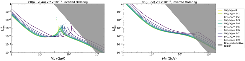
Figure B.6: Constraints for a degenerate and hierarchical HNL mass spectrum for two different processes (showed at the top of the plot): muon conversion in Gold (left) and $\mu\to 3e$ (right).

B.4 Loop functions

For completeness we also show the relevant loop integrals that appear in the expression (35–40):

$$F_{\gamma}(x)= \frac{7x^{3}-x^{2}-12x}{12(1-x)^{3}}-\frac{x^{4}-10x^{3}+12x^{2}}{6(1-x)^{4}}\log x\,,$$ (43)

$$G_{\gamma}(x)= -\frac{x(2x^{2}+5x-1)}{4(1-x)^{3}}-\frac{3x^{3}}{2(1-x)^{4}}\log x\,,$$ (44)

$$F_{Z}(x)= -\frac{5x}{2(1-x)}-\frac{5x^{2}}{2(1-x)^{2}}\log x\,,$$ (45)

$$G_{Z}(x,y)= -\frac{1}{2(x-y)}\left[\frac{x^{2}(1-y)}{1-x}\log x-\frac{y^{2}(1-x)}{1-y}\log y\right]\,,$$ (46)

$$H_{Z}(x,y)= \frac{\sqrt{xy}}{4(x-y)}\left[\frac{x^{2}-4x}{1-x}\log x-\frac{y^{2}-4y}{1-y}\log y\ \right]\,,$$ (47)

$$F_{\text{box}}(x,y)= \begin{aligned} &\frac{1}{x-y}\left\{\left(4+\frac{xy}{4}\right)\left[\frac{1}{1-x}+\frac{x^{2}}{(1-x)^{2}}\log x-\frac{1}{1-y}-\frac{y^{2}}{(1-y)^{2}}\log y\right]\right.\\ &\left.-2xy\left[\frac{1}{1-x}+\frac{x}{(1-x)^{2}}\log x-\frac{1}{1-y}-\frac{y}{(1-y)^{2}}\log y\right]\right\}\,\end{aligned}$$ (48)

$$F_{\text{Xbox}}(x,y)= \begin{aligned} &-\frac{1}{x-y}\left\{\left(1+\frac{xy}{4}\right)\left[\frac{1}{1-x}+\frac{x^{2}}{(1-x)^{2}}\log x-\frac{1}{1-y}-\frac{y^{2}}{(1-y)^{2}}\log y\right]\right.\\ &\left.-2xy\left[\frac{1}{1-x}+\frac{x}{(1-x)^{2}}\log x-\frac{1}{1-y}-\frac{y}{(1-y)^{2}}\log y\right]\right\}\,,\end{aligned}$$ (49)

$$G_{\text{box}}(x,y)= \begin{aligned} &-\frac{\sqrt{xy}}{x-y}\left\{(4+xy)\left[\frac{1}{1-x}+\frac{x}{(1-x)^{2}}\log x-\frac{1}{1-y}-\frac{y}{(1-y)^{2}}\log y\right]\right.\\ &\left.-2\left[\frac{1}{1-x}+\frac{x^{2}}{(1-x)^{2}}\log x-\frac{1}{1-y}-\frac{y^{2}}{(1-y)^{2}}\log y\right]\right\}\,.\\ \end{aligned}$$ (50)

B.5 Asymptotic behaviour of branching ratios

Using the formulas defined in Appendix B.4, we can extract the behaviour of branching ratios (24–27) for large masses $x=(M_{N}/m_{W})^{2}\gg 1$.

$$\mathrm{BR}(\ell_{\beta}\to 3\ell_{\alpha}) \propto\begin{aligned} &U_{\mathrm{tot}}^{8}\biggl{[}x^{2}\left(\frac{1}{2}-2s_{w}^{2}+3s_{w}^{4}-\frac{1}{2}\lambda_{\alpha}+s_{w}^{2}\lambda_{\alpha}+\frac{1}{8}\lambda_{\alpha}^{2}\right)\\ &\quad+x\log x\,\lambda_{\alpha}\left(-3+6\,s_{w}^{2}+\frac{3}{2}\lambda_{\alpha}\right)+\frac{9}{2}(\log x)^{2}\lambda_{\alpha}^{2}\biggr{]}\\ &+U_{\mathrm{tot}}^{6}\biggl{[}x\log x\left(3-\frac{34}{3}s_{w}^{2}+16s_{w}^{4}-\frac{3}{2}s_{w}^{2}\lambda_{\alpha}+\frac{8}{3}s_{w}^{4}\lambda_{\alpha}\right)\\ &\quad+(\log x)^{2}\,(12s_{w}^{2}-9)\,\lambda_{\alpha}\biggr{]}+U_{\mathrm{tot}}^{4}(\log x)^{2}\left(\frac{9}{2}-16s_{w}^{2}+\frac{64}{3}s_{w}^{4}\right)\,,\end{aligned}$$ (51)

$$\begin{split}\mathrm{CR}(\mu-e,\,\mathrm{A})&\propto\Bigl{|}U_{\mathrm{tot}}^{4}\,x\,(3-8s_{w}^{2})\left(V^{(n)}_{\mathrm{A}}-V^{(p)}_{\mathrm{A}}\right)\\ &\quad+U_{\mathrm{tot}}^{2}\log x\left[V^{(n)}_{\mathrm{A}}\left(9-24s_{w}^{2}\right)-V^{(p)}_{\mathrm{A}}\left(9-20s_{w}^{2}\right)\right]\Bigr{|}^{2}\,,\end{split}$$ (52)

We have only considered the leading terms in $x$ for each power of ${U}_{\mathrm{tot}}$ in equations (51–52), there are additional powers of $x$ that are not negligible and should be taken into consideration when doing any calculation regarding them.

Equations (25–26) also show a similar asymptotic behaviour to that of (24), as they also have contributions coming from $Z$-penguins and HNL box diagrams. The decays these formulas describe ($\tau\to\mu\mu e,\tau\to ee\mu$) are not as constrained as muon decays and were not examined, but they do offer an interesting opportunity to probe all mixing angles since these decays require HNLs to couple to all lepton flavors.

Appendix C Feynman diagrams contributing to the relevant processes

We show below all the relevant Feynman diagrams of the processes we highlighted. All are in the Feynman-’t Hooft gauge and therefore contain intermediate Goldstone bosons. The diagrams containing divergences have their respective letter in red, and the ones that exhibit the non-decoupling behavior highlighted in the main text are in green.

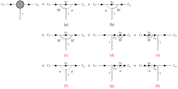
Figure C.7: Diagrams contributing to the $\gamma\ell_{\alpha}\ell_{\beta}$ vertex. To this vertex there are no two-HNL contributions. The diagrams with red labels have an UV divergence that ultimately vanishes.

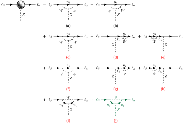
Figure C.8: Diagrams contributing to the $Z\ell_{\alpha}\ell_{\beta}$ vertex. The diagrams in green are new, accounting for two-HNL interactions. The diagrams with red labels have an UV divergence that ultimately vanishes.

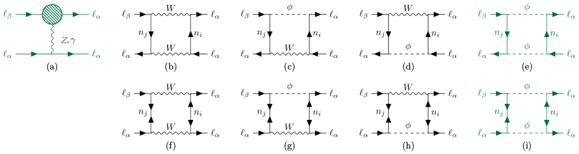
Figure C.9: Diagrams contributing to the $\ell_{\beta}\to 3\ell_{\alpha}$ decay. The diagrams in green are new, accounting for two-HNL interactions. Notice that some of the two HNL contributions, coming from $Zn_{i}n_{j}$ are hidden inside the “blob” of the diagram (a) (given by the diagram C.8).

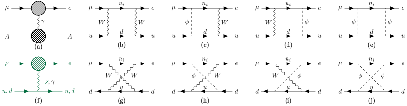
Figure C.10: Diagrams contributing to muon conversion in a nucleus decay. The diagrams in green are new, accounting for two-HNL interactions. Notice that in this case all two HNL contributions are inside the “blob” of the diagram (f) coupling to $Z$-bosons (given by the diagram C.8), which explains its color.

Appendix D Higher order terms

Figure D.11: Example of two-loop diagrams contributing to $\ell_{\beta}\to 3\ell_{\alpha}$

A complete computation of all two-loop diagrams of all non-decoupling processs is beyond the scope of this work, but by looking at the parameter dependence of the amplitude of the leading two-loop non-decoupling diagrams, one can get an idea of how the calculation will be validity of the supposition by keeping $Y<4\pi$, the theory remains perturbative.

Indeed, by finding the parametric dependence of both diagrams in Fig. D.11 we find that:

$$\mathcal{M}_{\mathrm{2-loop}}=\Theta^{2}\left(\frac{Y^{2}}{16\pi^{2}}\right)^{2}\,,$$ (53)

where the $16\pi^{2}$ is the usual term one gets when doing the four dimensional loop integrals, which in case of a two-loop diagram it should be squared, of course. This is in direct comparison with the parametric dependence of the leading order terms of one-loop diagrams:

$$\mathcal{M}=\Theta^{2}\left[\frac{Y^{2}}{16\pi^{2}}+\left(\frac{Y^{2}}{16\pi^{2}}\right)^{2}\right]\,,$$ (54)

The two-loop amplitude will be smaller than the one-loop one as long as $Y<4\pi$, which is in complete accordance with the classical perturbative limit for Yukawa couplings. One should expect the higher order ones to follow a similar dependence on Yukawas and a suppression of $16\pi^{2}$.

References

- (1) Particle Data Group collaboration, Review of Particle Physics, PTEP 2020 (2020) 083C01.
- (2) A. de Gouvêa, Neutrino Mass Models, Ann. Rev. Nucl. Part. Sci. 66 (2016) 197.
- (3) P. Minkowski, at a Rate of One Out of Muon Decays?, Phys. Lett. B 67 (1977) 421.
- (4) T. Yanagida, Horizontal Gauge Symmetry and Masses of Neutrinos, Conf. Proc. C 7902131 (1979) 95.
- (5) S.L. Glashow, The Future of Elementary Particle Physics, NATO Sci. Ser. B 61 (1980) 687.
- (6) M. Gell-Mann, P. Ramond and R. Slansky, Complex Spinors and Unified Theories, Conf. Proc. C 790927 (1979) 315 [1306.4669].
- (7) R.N. Mohapatra and G. Senjanovic, Neutrino Mass and Spontaneous Parity Nonconservation, Phys. Rev. Lett. 44 (1980) 912.
- (8) R.N. Mohapatra and G. Senjanovic, Neutrino Masses and Mixings in Gauge Models with Spontaneous Parity Violation, Phys. Rev. D 23 (1981) 165.
- (9) J. Schechter and J.W.F. Valle, Neutrino Masses in U(1) Theories, Phys. Rev. D 22 (1980) 2227.
- (10) J. Schechter and J.W.F. Valle, Neutrino Decay and Spontaneous Violation of Lepton Number, Phys. Rev. D 25 (1982) 774.
- (11) I. Esteban, M.C. Gonzalez-Garcia, M. Maltoni, T. Schwetz and A. Zhou, The Fate of Hints: Updated Global Analysis of Three-Flavor Neutrino Oscillations, JHEP 09 (2020) 178 [2007.14792].
- (12) P. Agrawal et al., Feebly-Interacting Particles: Fips 2020 Workshop Report, Eur. Phys. J. C 81 (2021) 1015 [2102.12143].
- (13) A.M. Abdullahi et al., The Present and Future Status of Heavy Neutral Leptons, in 2022 Snowmass Summer Study, 3, 2022 [2203.08039].
- (14) N. Sabti, A. Magalich and A. Filimonova, An Extended Analysis of Heavy Neutral Leptons during Big Bang Nucleosynthesis, JCAP 11 (2020) 056 [2006.07387].
- (15) A. Boyarsky, M. Ovchynnikov, O. Ruchayskiy and V. Syvolap, Improved Big Bang Nucleosynthesis Constraints on Heavy Neutral Leptons, Phys. Rev. D 104 (2021) 023517 [2008.00749].
- (16) K. Bondarenko, A. Boyarsky, J. Klaric, O. Mikulenko, O. Ruchayskiy, V. Syvolap et al., An Allowed Window for Heavy Neutral Leptons Below the Kaon Mass, JHEP 07 (2021) 193 [2101.09255].
- (17) M. Fukugita and T. Yanagida, Resurrection of Grand Unified Theory Baryogenesis, Phys. Rev. Lett. 89 (2002) 131602 [hep-ph/0203194].
- (18) S. Davidson, E. Nardi and Y. Nir, Leptogenesis, Phys. Rept. 466 (2008) 105 [0802.2962].
- (19) A. Pilaftsis, The Little Review on Leptogenesis, J. Phys. Conf. Ser. 171 (2009) 012017 [0904.1182].
- (20) M. Shaposhnikov, Baryogenesis, J. Phys. Conf. Ser. 171 (2009) 012005.
- (21) W. Buchmuller, P. Di Bari and M. Plumacher, Leptogenesis for pedestrians, Annals Phys. 315 (2005) 305 [hep-ph/0401240].
- (22) D. Bodeker and W. Buchmuller, Baryogenesis from the Weak Scale to the Grand Unification Scale, Rev. Mod. Phys. 93 (2021) 035004 [2009.07294].
- (23) E.K. Akhmedov, V.A. Rubakov and A.Y. Smirnov, Baryogenesis via Neutrino Oscillations, Phys. Rev. Lett. 81 (1998) 1359 [hep-ph/9803255].
- (24) T. Asaka and M. Shaposhnikov, The MSM, dark matter and baryon asymmetry of the universe, Phys. Lett. B 620 (2005) 17 [hep-ph/0505013].
- (25) A. Pilaftsis and T.E.J. Underwood, Electroweak-Scale Resonant Leptogenesis, Phys. Rev. D 72 (2005) 113001 [hep-ph/0506107].
- (26) J. Klarić, M. Shaposhnikov and I. Timiryasov, Uniting Low-Scale Leptogenesis Mechanisms, Phys. Rev. Lett. 127 (2021) 111802 [2008.13771].
- (27) J. Klarić, M. Shaposhnikov and I. Timiryasov, Reconciling resonant leptogenesis and baryogenesis via neutrino oscillations, Phys. Rev. D 104 (2021) 055010 [2103.16545].
- (28) M. Drewes, Y. Georis and J. Klarić, Mapping the Viable Parameter Space for Testable Leptogenesis, Phys. Rev. Lett. 128 (2022) 051801 [2106.16226].
- (29) D. Wyler and L. Wolfenstein, Massless Neutrinos in Left-Right Symmetric Models, Nucl. Phys. B 218 (1983) 205.
- (30) C.N. Leung and S.T. Petcov, A Comment on the Coexistence of Dirac and Majorana Massive Neutrinos, Phys. Lett. B 125 (1983) 461.
- (31) R.N. Mohapatra and J.W.F. Valle, Neutrino Mass and Baryon Number Nonconservation in Superstring Models, Phys. Rev. D 34 (1986) 1642.
- (32) G.C. Branco, W. Grimus and L. Lavoura, The Seesaw Mechanism in the Presence of a Conserved Lepton Number, Nucl. Phys. B 312 (1989) 492.
- (33) M.C. Gonzalez-Garcia and J.W.F. Valle, Fast Decaying Neutrinos and Observable Flavor Violation in a New Class of Majoron Models, Phys. Lett. B 216 (1989) 360.
- (34) M. Shaposhnikov, A Possible Symmetry of the Numsm, Nucl. Phys. B 763 (2007) 49 [hep-ph/0605047].
- (35) J. Kersten and A.Y. Smirnov, Right-Handed Neutrinos at CERN LHC and the Mechanism of Neutrino Mass Generation, Phys. Rev. D 76 (2007) 073005 [0705.3221].
- (36) A. Abada, C. Biggio, F. Bonnet, M.B. Gavela and T. Hambye, Low Energy Effects of Neutrino Masses, JHEP 12 (2007) 061 [0707.4058].
- (37) M.B. Gavela, T. Hambye, D. Hernandez and P. Hernandez, Minimal Flavour Seesaw Models, JHEP 09 (2009) 038 [0906.1461].
- (38) K. Moffat, S. Pascoli and C. Weiland, Equivalence Between Massless Neutrinos and Lepton Number Conservation in Fermionic Singlet Extensions of the Standard Model, 1712.07611.
- (39) M. Drewes, J. Klarić and P. Klose, On lepton number violation in heavy neutrino decays at colliders, JHEP 11 (2019) 032 [1907.13034].
- (40) L. Wolfenstein, Different Varieties of Massive Dirac Neutrinos, Nucl. Phys. B 186 (1981) 147.
- (41) S.T. Petcov, On Pseudodirac Neutrinos, Neutrino Oscillations and Neutrinoless Double Beta Decay, Phys. Lett. B 110 (1982) 245.
- (42) C.N. Leung and J.L. Rosner, Neutral Massive Leptons in an SO(10) Model With Massless Neutrinos, Phys. Rev. D 28 (1983) 2205.
- (43) M. Gronau, C.N. Leung and J.L. Rosner, Extending Limits on Neutral Heavy Leptons, Phys. Rev. D29 (1984) 2539.
- (44) F. del Aguila, J.A. Aguilar-Saavedra and R. Pittau, Heavy neutrino signals at large hadron colliders, JHEP 10 (2007) 047 [hep-ph/0703261].
- (45) G. Cvetic, C. Dib, S.K. Kang and C.S. Kim, Probing Majorana neutrinos in rare and meson decays, Phys. Rev. D 82 (2010) 053010 [1005.4282].
- (46) G. Cvetic, C. Dib and C.S. Kim, Probing Majorana neutrinos in rare decays, JHEP 06 (2012) 149 [1203.0573].
- (47) D. Alva, T. Han and R. Ruiz, Heavy Majorana neutrinos from fusion at hadron colliders, JHEP 02 (2015) 072 [1411.7305].
- (48) S. Pascoli, R. Ruiz and C. Weiland, Heavy neutrinos with dynamic jet vetoes: multilepton searches at , 27, and 100 TeV, JHEP 06 (2019) 049 [1812.08750].
- (49) B. Fuks, J. Neundorf, K. Peters, R. Ruiz and M. Saimpert, Majorana neutrinos in same-sign scattering at the LHC: Breaking the TeV barrier, Phys. Rev. D 103 (2021) 055005 [2011.02547].
- (50) S.T. Petcov, The Processes in the Weinberg-Salam Model with Neutrino Mixing, Sov. J. Nucl. Phys. 25 (1977) 340.
- (51) S.M. Bilenky, S.T. Petcov and B. Pontecorvo, Lepton Mixing, mu – e + gamma Decay and Neutrino Oscillations, Phys. Lett. B 67 (1977) 309.
- (52) W.J. Marciano and A.I. Sanda, Exotic Decays of the Muon and Heavy Leptons in Gauge Theories, Phys. Lett. B 67 (1977) 303.
- (53) T.P. Cheng and L.-F. Li, in Theories With Dirac and Majorana Neutrino Mass Terms, Phys. Rev. Lett. 45 (1980) 1908.
- (54) C.S. Lim and T. Inami, Lepton Flavor Nonconservation and the Mass Generation Mechanism for Neutrinos, Prog. Theor. Phys. 67 (1982) 1569.
- (55) P. Langacker and D. London, Lepton Number Violation and Massless Nonorthogonal Neutrinos, Phys. Rev. D 38 (1988) 907.
- (56) A. Pilaftsis, Lepton flavor nonconservation in H0 decays, Phys. Lett. B 285 (1992) 68.
- (57) A. Ilakovac and A. Pilaftsis, Flavor violating charged lepton decays in seesaw-type models, Nucl. Phys. B 437 (1995) 491 [hep-ph/9403398].
- (58) J.I. Illana, M. Jack and T. Riemann, Predictions for Z — mu tau and related reactions, in 2nd Workshop of the 2nd Joint ECFA / DESY Study on Physics and Detectors for a Linear Electron Positron Collider, pp. 490–524, 12, 1999 [hep-ph/0001273].
- (59) J.I. Illana and T. Riemann, Charged lepton flavor violation from massive neutrinos in Z decays, Phys. Rev. D 63 (2001) 053004 [hep-ph/0010193].
- (60) S. Pascoli, S.T. Petcov and C.E. Yaguna, Quasidegenerate neutrino mass spectrum, mu — e + gamma decay and leptogenesis, Phys. Lett. B 564 (2003) 241 [hep-ph/0301095].
- (61) S. Pascoli, S.T. Petcov and W. Rodejohann, On the Connection of Leptogenesis with Low-Energy CP Violation and Lfv Charged Lepton Decays, Phys. Rev. D 68 (2003) 093007 [hep-ph/0302054].
- (62) E. Arganda, A.M. Curiel, M.J. Herrero and D. Temes, Lepton flavor violating Higgs boson decays from massive seesaw neutrinos, Phys. Rev. D 71 (2005) 035011 [hep-ph/0407302].
- (63) D. Gorbunov and I. Timiryasov, Testing MSM with indirect searches, Phys. Lett. B 745 (2015) 29 [1412.7751].
- (64) E. Arganda, M.J. Herrero, X. Marcano, R. Morales and A. Szynkman, Effective lepton flavor violating Hij vertex from right-handed neutrinos within the mass insertion approximation, Phys. Rev. D 95 (2017) 095029 [1612.09290].
- (65) A. Abada, V. De Romeri and A.M. Teixeira, Impact of sterile neutrinos on nuclear-assisted cLFV processes, JHEP 02 (2016) 083 [1510.06657].
- (66) P.D. Bolton and S.T. Petcov, Measurements of decay with polarised muons as a probe of new physics, Phys. Lett. B 833 (2022) 137296 [2204.03468].
- (67) A.-Y. Bai et al., Snowmass2021 Whitepaper: Muonium to antimuonium conversion, in 2022 Snowmass Summer Study, 3, 2022 [2203.11406].
- (68) A. de Gouvêa and A. Kobach, Global Constraints on a Heavy Neutrino, Phys. Rev. D 93 (2016) 033005 [1511.00683].
- (69) E. Fernandez-Martínez, J. Hernandez-Garcia and J. Lopez-Pavon, Global Constraints on Heavy Neutrino Mixing, JHEP 08 (2016) 033 [1605.08774].
- (70) R.H. Bernstein and P.S. Cooper, Charged Lepton Flavor Violation: an Experimenter’s Guide, Phys. Rept. 532 (2013) 27 [1307.5787].
- (71) L. Calibbi and G. Signorelli, Charged Lepton Flavour Violation: an Experimental and Theoretical Introduction, Riv. Nuovo Cim. 41 (2018) 71 [1709.00294].
- (72) P.D. Bolton, F.F. Deppisch and P.S. Bhupal Dev, Neutrinoless double beta decay versus other probes of heavy sterile neutrinos, JHEP 03 (2020) 170 [1912.03058].
- (73) CMS collaboration, Probing heavy Majorana neutrinos and the Weinberg operator through vector boson fusion processes in proton-proton collisions at = 13 TeV, 2206.08956.
- (74) S.T. Petcov, The Nature of Massive Neutrinos, Adv. High Energy Phys. 2013 (2013) 852987 [1303.5819].
- (75) A. Denner, H. Eck, O. Hahn and J. Kublbeck, Feynman rules for fermion number violating interactions, Nucl. Phys. B 387 (1992) 467.
- (76) J.A. Casas and A. Ibarra, Oscillating neutrinos and , Nucl. Phys. B 618 (2001) 171 [hep-ph/0103065].
- (77) A. Ibarra and G.G. Ross, Neutrino Phenomenology: the Case of Two Right-Handed Neutrinos, Phys. Lett. B 591 (2004) 285 [hep-ph/0312138].
- (78) S.T. Petcov, W. Rodejohann, T. Shindou and Y. Takanishi, The See-saw mechanism, neutrino Yukawa couplings, LFV decays l(i) — l(j) + gamma and leptogenesis, Nucl. Phys. B 739 (2006) 208 [hep-ph/0510404].
- (79) S. Eijima, M. Shaposhnikov and I. Timiryasov, Parameter space of baryogenesis in the MSM, JHEP 07 (2019) 077 [1808.10833].
- (80) M.A. Shifman, Foreword to Itep Lectures in Particle Physics, 10, 1995 [hep-ph/9510397].
- (81) T. Appelquist and J. Carazzone, Infrared Singularities and Massive Fields, Phys. Rev. D 11 (1975) 2856.
- (82) J.C. Collins, F. Wilczek and A. Zee, Low-Energy Manifestations of Heavy Particles: Application to the Neutral Current, Phys. Rev. D 18 (1978) 242.
- (83) T.P. Cheng and L.-F. Li, Effects of Superheavy Neutrinos in Low-Energy Weak Processes, Phys. Rev. D 44 (1991) 1502.
- (84) D. Tommasini, G. Barenboim, J. Bernabeu and C. Jarlskog, Nondecoupling of heavy neutrinos and lepton flavor violation, Nucl. Phys. B 444 (1995) 451 [hep-ph/9503228].
- (85) E. D’Hoker and E. Farhi, Decoupling a Fermion in the Standard Electroweak Theory, Nucl. Phys. B 248 (1984) 77.
- (86) E. D’Hoker and E. Farhi, Decoupling a Fermion Whose Mass Is Generated by a Yukawa Coupling: The General Case, Nucl. Phys. B 248 (1984) 59.
- (87) J.C. Collins, Renormalization: An Introduction to Renormalization, The Renormalization Group, and the Operator Product Expansion, vol. 26 of Cambridge Monographs on Mathematical Physics, Cambridge University Press, Cambridge (1986), 10.1017/CBO9780511622656.
- (88) M.S. Chanowitz, M.A. Furman and I. Hinchliffe, Weak Interactions of Ultraheavy Fermions. 2., Nucl. Phys. B 153 (1979) 402.
- (89) L. Durand, J.M. Johnson and J.L. Lopez, Perturbative Unitarity Revisited: A New Upper Bound on the Higgs Boson Mass, Phys. Rev. Lett. 64 (1990) 1215.
- (90) S. Fajfer and A. Ilakovac, Lepton flavor violation in light hadron decays, Phys. Rev. D 57 (1998) 4219.
- (91) S. Ipek, A.D. Plascencia and J. Turner, Assessing Perturbativity and Vacuum Stability in High-Scale Leptogenesis, JHEP 12 (2018) 111 [1806.00460].
- (92) D. Zhang and S. Zhou, Complete One-Loop Matching of the Type-I Seesaw Model Onto the Standard Model Effective Field Theory, JHEP 09 (2021) 163 [2107.12133].
- (93) SINDRUM II collaboration, A Search for muon to electron conversion in muonic gold, Eur. Phys. J. C 47 (2006) 337.
- (94) R. Alonso, M. Dhen, M.B. Gavela and T. Hambye, Muon Conversion to Electron in Nuclei in Type-I Seesaw Models, JHEP 01 (2013) 118 [1209.2679].
- (95) A. Abada and A.M. Teixeira, Heavy neutral leptons and high-intensity observables, Front. in Phys. 6 (2018) 142 [1812.08062].
- (96) J.-L. Tastet, O. Ruchayskiy and I. Timiryasov, Reinterpreting the Atlas Bounds on Heavy Neutral Leptons in a Realistic Neutrino Oscillation Model, JHEP 12 (2021) 182 [2107.12980].
- (97) CMS collaboration, Search for heavy neutral leptons in events with three charged leptons in proton-proton collisions at 13 TeV, Phys. Rev. Lett. 120 (2018) 221801 [1802.02965].
- (98) ATLAS collaboration, Search for heavy neutral leptons in decays of bosons produced in 13 TeV collisions using prompt and displaced signatures with the ATLAS detector, JHEP 10 (2019) 265 [1905.09787].
- (99) CMS collaboration, Search for long-lived heavy neutral leptons with displaced vertices in proton-proton collisions at =13 TeV, 2201.05578.
- (100) ATLAS collaboration, Search for heavy neutral leptons in decays of bosons using a dilepton displaced vertex in TeV collisions with the ATLAS detector, 2204.11988.
- (101) S. Mihara, J.P. Miller, P. Paradisi and G. Piredda, Charged Lepton Flavor-Violation Experiments, Ann. Rev. Nucl. Part. Sci. 63 (2013) 531.
- (102) C. Group collaboration, A New Charged Lepton Flavor Violation Program at Fermilab, in 2022 Snowmass Summer Study, 3, 2022 [2203.08278].
- (103) SHiP collaboration, Sensitivity of the Ship Experiment to Heavy Neutral Leptons, JHEP 04 (2019) 077 [1811.00930].
- (104) FCC-ee study Team collaboration, Search for Heavy Right Handed Neutrinos at the FCC-ee, Nucl. Part. Phys. Proc. 273-275 (2016) 1883 [1411.5230].
- (105) X. Chu, M. Dhen and T. Hambye, Relations among neutrino observables in the light of a large angle, JHEP 11 (2011) 106 [1107.1589].
- (106) T. Hambye, Clfv and the Origin of Neutrino Masses, Nucl. Phys. B Proc. Suppl. 248-250 (2014) 13 [1312.5214].
- (107) R.N. Mohapatra, Mechanism for Understanding Small Neutrino Mass in Superstring Theories, Phys. Rev. Lett. 56 (1986) 561.
- (108) J. Bernabeu, A. Santamaria, J. Vidal, A. Mendez and J.W.F. Valle, Lepton Flavor Nonconservation at High-Energies in a Superstring Inspired Standard Model, Phys. Lett. B 187 (1987) 303.
- (109) E.K. Akhmedov, M. Lindner, E. Schnapka and J.W.F. Valle, Left-right symmetry breaking in NJL approach, Phys. Lett. B 368 (1996) 270 [hep-ph/9507275].
- (110) E.K. Akhmedov, M. Lindner, E. Schnapka and J.W.F. Valle, Dynamical left-right symmetry breaking, Phys. Rev. D 53 (1996) 2752 [hep-ph/9509255].
- (111) R.B. Patterson, Prospects for Measurement of the Neutrino Mass Hierarchy, Ann. Rev. Nucl. Part. Sci. 65 (2015) 177 [1506.07917].
- (112) DUNE collaboration, Low Exposure Long-Baseline Neutrino Oscillation Sensitivity of the Dune Experiment, Phys. Rev. D 105 (2022) 072006 [2109.01304].
- (113) D. Foreman-Mackey, D.W. Hogg, D. Lang and J. Goodman, emcee: The MCMC Hammer, Publ. Astron. Soc. Pac. 125 (2013) 306 [1202.3665].
- (114) A. Lewis, GetDist: a Python package for analysing Monte Carlo samples, 1910.13970.
- (115) MEG collaboration, Search for the lepton flavour violating decay with the full dataset of the MEG experiment, Eur. Phys. J. C 76 (2016) 434 [1605.05081].
- (116) MEG II collaboration, The design of the MEG II experiment, Eur. Phys. J. C 78 (2018) 380 [1801.04688].
- (117) SINDRUM collaboration, Search for the Decay mu+ — e+ e+ e-, Nucl. Phys. B 299 (1988) 1.
- (118) A. Blondel et al., Research Proposal for an Experiment to Search for the Decay , 1301.6113.
- (119) Mu3e collaboration, The Mu3e Experiment, Nucl. Phys. B Proc. Suppl. 248-250 (2014) 35.
- (120) SINDRUM II collaboration, Test of lepton flavor conservation in mu — e conversion on titanium, Phys. Lett. B 317 (1993) 631.
- (121) Mu2e collaboration, Mu2E Technical Design Report, 1501.05241.
- (122) COMET collaboration, COMET Phase-I Technical Design Report, PTEP 2020 (2020) 033C01 [1812.09018].
- (123) SINDRUM II collaboration, Improved limit on the branching ratio of mu — e conversion on lead, Phys. Rev. Lett. 76 (1996) 200.
- (124) ATLAS collaboration, Search for the lepton flavor violating decay Z→e in pp collisions at TeV with the ATLAS detector, Phys. Rev. D 90 (2014) 072010 [1408.5774].
- (125) M. Dam, Tau-lepton Physics at the FCC-ee circular e+e- Collider, SciPost Phys. Proc. 1 (2019) 041 [1811.09408].
- (126) ATLAS collaboration, Search for the Higgs boson decays and in collisions at TeV with the ATLAS detector, Phys. Lett. B 801 (2020) 135148 [1909.10235].
- (127) BaBar collaboration, Searches for Lepton Flavor Violation in the Decays tau+- — e+- gamma and tau+- — mu+- gamma, Phys. Rev. Lett. 104 (2010) 021802 [0908.2381].
- (128) Belle-II collaboration, The Belle II Physics Book, PTEP 2019 (2019) 123C01 [1808.10567].
- (129) K. Hayasaka et al., Search for Lepton Flavor Violating Tau Decays into Three Leptons with 719 Million Produced Tau+Tau- Pairs, Phys. Lett. B 687 (2010) 139 [1001.3221].
- (130) OPAL collaboration, A Search for lepton flavor violating Z0 decays, Z. Phys. C 67 (1995) 555.
- (131) ATLAS collaboration, Searches for lepton-flavour-violating decays of the Higgs boson in TeV pp collisions with the ATLAS detector, Phys. Lett. B 800 (2020) 135069 [1907.06131].
- (132) DELPHI collaboration, Search for lepton flavor number violating Z0 decays, Z. Phys. C 73 (1997) 243.
- (133) CMS collaboration, Search for lepton flavour violating decays of the Higgs boson to and e in proton-proton collisions at 13 TeV, JHEP 06 (2018) 001 [1712.07173].
- (134) A. Granelli, J. Klarić and S.T. Petcov, Tests of Low-Scale Leptogenesis in Charged Lepton Flavour Violation Experiments, 2206.04342.
- (135) A. Abada, J. Kriewald and A.M. Teixeira, On the role of leptonic CPV phases in cLFV observables, Eur. Phys. J. C 81 (2021) 1016 [2107.06313].
- (136) S. Alekhin et al., A Facility to Search for Hidden Particles at the Cern Sps: the Ship Physics Case, Rept. Prog. Phys. 79 (2016) 124201 [1504.04855].
- (137) J. Beacham et al., Physics Beyond Colliders at Cern: Beyond the Standard Model Working Group Report, J. Phys. G 47 (2020) 010501 [1901.09966].
- (138) R.K. Ellis et al., Physics Briefing Book: Input for the European Strategy for Particle Physics Update 2020, 1910.11775.
- (139) C.C. Ahdida et al., Sps Beam Dump Facility - Comprehensive Design Study, vol. 2/2020 of CERN Yellow Reports: Monographs (2020), 10.23731/CYRM-2020-002, [1912.06356].
- (140) F. Kirk, Flavour-violating leptonic decays in the MSM, Master’s thesis, Ecole Polytechnique Federale de Lausanne, 7, 2015.
- (141) V. Shtabovenko, R. Mertig and F. Orellana, FeynCalc 9.3: New features and improvements, Comput. Phys. Commun. 256 (2020) 107478 [2001.04407].
- (142) T. Hahn, Generating Feynman diagrams and amplitudes with FeynArts 3, Comput. Phys. Commun. 140 (2001) 418 [hep-ph/0012260].
- (143) H.H. Patel, Package-X 2.0: A Mathematica package for the analytic calculation of one-loop integrals, Comput. Phys. Commun. 218 (2017) 66 [1612.00009].
- (144) Riazuddin, R.E. Marshak and R.N. Mohapatra, Majorana Neutrinos and Low-Energy Tests of Electroweak Models, Phys. Rev. D 24 (1981) 1310.
- (145) L.N. Chang, D. Ng and J.N. Ng, Phenomenological Consequences of Singlet Neutrinos, Phys. Rev. D 50 (1994) 4589 [hep-ph/9402259].
- (146) A. Pilaftsis, Heavy Majorana Neutrinos and Baryogenesis, Int. J. Mod. Phys. A 14 (1999) 1811 [hep-ph/9812256].
- (147) A. Ioannisian and A. Pilaftsis, Cumulative Nondecoupling Effects of Kaluza-Klein Neutrinos in Electroweak Processes, Phys. Rev. D 62 (2000) 066001 [hep-ph/9907522].
- (148) F. Deppisch, T.S. Kosmas and J.W.F. Valle, Enhanced Mu- - E- Conversion in Nuclei in the Inverse Seesaw Model, Nucl. Phys. B 752 (2006) 80 [hep-ph/0512360].
- (149) F.F. Deppisch and A. Pilaftsis, Lepton Flavour Violation and Theta(13) in Minimal Resonant Leptogenesis, Phys. Rev. D 83 (2011) 076007 [1012.1834].
- (150) C. Degrande, O. Mattelaer, R. Ruiz and J. Turner, Fully-Automated Precision Predictions for Heavy Neutrino Production Mechanisms at Hadron Colliders, Phys. Rev. D 94 (2016) 053002 [1602.06957].
- (151) R. Ruiz, “SM + Heavy N at NLO In QCD.”
- (152) K.A. Urquía-Calderón, “HeavyN mass basis.” Available at https://github.com/kurquia/heavyN_mass_basis, 2023.
- (153) R. Kitano, M. Koike and Y. Okada, Detailed calculation of lepton flavor violating muon electron conversion rate for various nuclei, Phys. Rev. D 66 (2002) 096002 [hep-ph/0203110].
- (154) J.G. Korner, A. Pilaftsis and K. Schilcher, Leptonic flavor changing Z0 decays in SU(2) x U(1) theories with right-handed neutrinos, Phys. Lett. B 300 (1993) 381 [hep-ph/9301290].
- (155) J.G. Korner, A. Pilaftsis and K. Schilcher, Leptonic CP asymmetries in flavor changing H0 decays, Phys. Rev. D 47 (1993) 1080 [hep-ph/9301289].
- (156) N.H. Thao, L.T. Hue, H.T. Hung and N.T. Xuan, Lepton flavor violating Higgs boson decays in seesaw models: new discussions, Nucl. Phys. B 921 (2017) 159 [1703.00896].
- (157) A. Pilaftsis, Radiatively induced neutrino masses and large Higgs neutrino couplings in the standard model with Majorana fields, Z. Phys. C 55 (1992) 275 [hep-ph/9901206].
- (158) B. Yu and S. Zhou, Sufficient and Necessary Conditions for CP Conservation in the Case of Degenerate Majorana Neutrino Masses, Phys. Rev. D 103 (2021) 035017 [2009.12347].