Convolutional Dictionary Learning by End-To-End Training of Iterative Neural Networks
Abstract
Sparsity-based methods have a long history in the field of signal processing and have been successfully applied to various image reconstruction problems. The involved sparsifying transformations or dictionaries are typically either pre-trained using a model which reflects the assumed properties of the signals or adaptively learned during the reconstruction - yielding so-called blind Compressed Sensing approaches. However, by doing so, the transforms are never explicitly trained in conjunction with the physical model which generates the signals. In addition, properly choosing the involved regularization parameters remains a challenging task. Another recently emerged training-paradigm for regularization methods is to use iterative neural networks (INNs) - also known as unrolled networks - which contain the physical model. In this work, we construct an INN which can be used as a supervised and physics-informed online convolutional dictionary learning algorithm. We evaluated the proposed approach by applying it to a realistic large-scale dynamic MR reconstruction problem and compared it to several other recently published works. We show that the proposed INN improves over two conventional model-agnostic training methods and yields competitive results also compared to a deep INN. Further, it does not require to choose the regularization parameters and - in contrast to deep INNs - each network component is entirely interpretable.
Index Terms:
Iterative Neural Networks, Sparsity, Convolutional Dictionary Learning, Compressed Sensing, Cardiac Cine MRII Introduction
Recently, image reconstruction has become an important application area of machine learning (ML) and has attracted the interest of researchers in different communities. The most prominent type of ML-approaches are so-called iterative neural networks (INNs) or unrolled networks, see e.g. [1], [2], [4]. INNs correspond to iterative reconstruction schemes of finite length and typically consists of regularizing blocks, e.g. convolutional layers, and so-called data-consistency blocks which make use of the forward and adjoint operators. Integrating the physical model into the network reduces the maximum error-bound [5] and improves the network in terms of generalization properties [6]. In addition, INNs were reported to be the most robust with respect to adversarial attacks compared to model-agnostic networks [7]. Despite their success, deep INNs are still black-boxes from a theoretical point of view. There is still no systematic way to design the employed convolutional blocks or to analyze them which raises concerns about their application in a sensitive field such as medical imaging. Nevertheless, the possibility to integrate the physical model into the learning process is a unique feature of INNs which distinguishes them from other learning-based methods which, on the other hand, often come with theoretical advantages such as convergence guarantees [8].
Convolutional dictionary learning (CDL) is a well-established approach which has been extensively applied to different tasks such as image denoising [8], image inpainting [9] and image reconstruction [10].
However, these methods typically learn the dictionary by solving the CDL-problem and are not necessarily tailored to the reconstruction algorithm they are subsequently used with. In addition, properly tuning the regularization parameters is crucial (as we shall see later in the experiments) and is often a tedious and difficult task.
In this work, we exploit the benefits of INNs - i.e. the inclusion of the physical model into the architecture - to construct a physics-informed and entirely interpretable ML-based regularization method using CDL. The proposed method corresponds to an unrolled reconstruction scheme using a learned convolutional dictionary. The filters of the convolutional dictionary as well as the involved regularization parameters - can then be trained in a supervised and physics-aware manner. We apply our method to a realistic large-scale dynamic MR image reconstruction problem and demonstrate that i) the filters obtained by the NN-training yield better reconstructions compared to the ones obtained by decoupled pre-training of the filters as in [8]
and [3] and ii) that the proposed method shows competitive results compared to a state-of-the-art method with deep iterative NNs [2].
II Methods
Our data measurement model corresponds to a general type of linear inverse problem
| (1) |
where models the measurement process, denotes the image, denotes Gaussian random noise and the measured data. The goal is to recover the unknown image from the observed measured data . Because such problems can be ill-posed for a variety of reasons, e.g. undersampling, poorly-conditioned systems or combinations thereof, the reconstruction requires the use of regularization methods which take additional information into account.
II-A Problem Formulation
Similar to [10], we consider the following regularized reconstruction problem
| (2) |
where denotes a set of fixed convolutional filters with for all and . Because the variables are linked with the convolution operator within the -norm and are also present within the non-smooth -norm, directly minimizing (2) is difficult. We therefore introduce auxiliary variables under the constraint for all , yielding the equivalent problem
| (3) | |||
Our aim is to set up a reconstruction algorithm based on (3) that defines a reconstruction network whose regularization parameters and filters are trained in an end-to-end manner.
II-B Reconstruction Algorithm
The proposed solution strategy is to define an alternating minimization scheme by minimizing (3) with respect to one of the variables by keeping the others fixed. For fixed , problem (3) takes the form of
| (4) | |||
for which we use the alternating direction method of multipliiers (ADMM) [11] to update and . For , the update-rules are given by
| (5) | |||
| (6) | |||
| (7) |
where are the dual-variables of the ADMM algorithm.
II-B1 Update of
Updating corresponds to the most challenging problem and is achieved by solving the sub-problem in the Fourier-domain. Define
| (8) |
Then, by making use of the Fourier-convolution theorem, updating according to (5) is equivalent to solving
| (9) |
where the multiplication is meant component-wise and . Problem (9) can be re-written in a more compact form as
| (10) |
where , and . Solving problem (10) corresponds to solving a linear system
| (11) |
which, because of its special structure, has a computationally inexpensive closed-form solution which can be obtained using the Sherman-Morrison formula, see [12] for more details. Let denote the solution of (10). Then we finally obtain for all as the solution of (5).
II-B2 Update of and
II-B3 Update of
Last, for fixed and , updating corresponds to solving the sub-problem
| (13) |
which can be achieved by solving the system with
| (14) | |||||
| (15) |
by any iterative solver, e.g. a conjugate gradient (CG)-method.
II-C Proposed Reconstruction Network
Note that the updates of the respective variables describe a solution strategy for solving problem (3) where the set of convolutional filters as well as the parameters , and are fixed. We construct a neural network whose blocks correspond to the operations required to solve the previously described sub-problems. Then, the filters as well as and are free parameters in the reconstruction network that can be learned by back-propagation on a set of input-target image pairs , where denotes a ground-truth image which is used as label during training and denotes an initial guess of the image which is typically directly obtained from the measured data by some reconstruction operator .
Typically, CDL algorithms impose a norm constraint on the filters, i.e. , to avoid the scaling ambiguity between the filters and the sparse coefficient maps [12], [8]. Since we train the filters by back-propagation, we project the filters onto the unit-sphere after each filter-update by rescaling them by the corresponding -norm.
II-D Implementation Details
Although the implementation of the single components of the proposed network might seem straight-forward at a first glance, a closer look at the sub-problems reveals that some of the operations require careful treatment. First, the Fourier-convolution theorem used to obtain (9) only holds when circular padding conditions are assumed. Second, from (9), one can see that the dimensionality of the filters in the Fourier-domain has to match the one of the image, which means that the filters have to be properly zero-padded. Third, to be able to use the Sherman-Morrison formula for solving (10), one needs to construct the right hand side of the system (11), where again, by proper circular and zero-padding, one needs to ensure that and therefore implicitly are indeeed the adjoint operators of and , respectively. This means that they need to fulfill and for all and . Last, because we treat complex-valued images as two-channeled images and the filters are shared across the real and the imaginary part, these aspects also have to be taken into account when constructing all relevant operators. An implementation of our network is available at www.github.com/koflera/ConvSparsityNNs.
III Experiments
We applied our proposed method to an accelerated cardiac cine MR image reconstruction problem using radial -space trajectories. The operator in (1) takes the form
| (16) |
for a complex valued image with , where denotes an identity operator and contains the coil-sensitivity maps, i.e. , with and . The operator consists of different 2D radial Fourier-encoding operators which for each time point sample a 2D image along radial lines in Fourier-space. To accelerate the acquisition process, we only acquire a sub-portion of the -space coefficients indexed by the set and denote the resulting operator by . The -space trajectories are chosen according to the golden-angle method and was implemented using the library TorchKBNufft [14]. Further, we used -space pre-conditioning, see [13] for more details.
III-A Dataset
We used a dataset of 15 healthy volunteers and four patients with a total of 216 cine MR images of shape . The data was split into 12/3/4 subjects (144/36/36 dynamic images) for training, validation and testing. The test set consisted of the four patients. As in [13], the initial -space data with coils was retrospectively simulated using spokes per cardiac phase and was corrupted by Gaussian noise with a standard deviation of resulting in an approximate SNR 8.5.
III-B 3D vs 2D
Because training INNs can be computationally demanding, we also consider a variant of problem (2), where instead of using 3D filters, we use 2D filters and impose the regularization for each time-frame, i.e. the regularization term in (2) changes to
| (17) |
This allows to use a larger number of filters during training at the price of not exploiting the temporal dimension for the regularization which is the one with the highest correlation among neighbouring pixels. Note that this formulation only changes the regularization term but not the reconstruction algorithm. Within the network, the temporal dimension of the image can be dynamically merged back and forth to play the role of the batch-dimension depending on the stage of the reconstruction.
III-C Methods of Comparison and Evaluation
Since our proposed approach is a method for training a convolutional dictionary, we compare it to two classical model-agnostic CDL-methods, which we refer to as CDL 2D and CDL 3D. For this, we pre-trained the 2D and 3D convolutional filters using [8] and [3] with and , respectively. After having obtained the filters, we fixed them in our network and only trained , and to exclude a possible change of performance which could be attributed to a sub-optimal choice of the regularization parameters. Further, we also compared with the method in [13], which corresponds to the analysis operator counterpart of this work and which we abbreviate by NN-CAOL 3D. We abbreviate our proposed methods by NN-CDL 3D and NN-CDL 2D, respectively. Last, we also compared our method to an adaptation of the deep cascade of CNNs presented in [2], which we denote by DnCn3D, see [13] for details. We trained all CDL-methods for different filter configurations with filters of shapes for 3D and with for 2D. Based on a hyper-parameter selection on the validation set, we finally used and for CDL 3D, NN-CDL 3D and CAOL 3D (see [13]), while for CDL 2D and NN-CDL 2D, we used and . The length of the networks and the number of CG-iterations for solving (14) were set to and for all CDL-methods. Because problem (2) is separable w.r.t. the temporal dimension, we trained all INNs on images only containing and cardiac phases for NN-CDL 2D and NN-CDL 3D, respectively. The INNs were trained for 16 epochs by minimizing the squared -error between the target image and the estimated one using ADAM with an initial learning rate of . All reconstructions were evaluated in terms of PSNR, NRMSE and SSIM which were calculated over a central squared ROI of pixels.
IV Results and Discussion
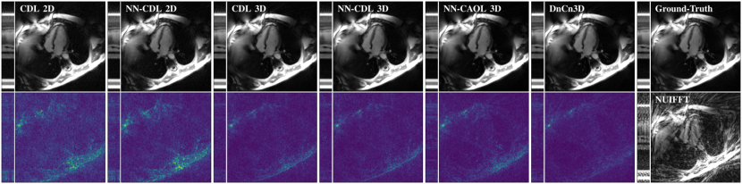
Figure 1 shows an example of images reconstructed by all used methods. All methods yielded accurate reconstructions by successfully removing undersampling artefacts and noise. By comparing CDL 2D to NN-CDL 2D and CDL 3D to NN-CDL 3D, we see that using the proposed INN resulted in a more accurate reconstruction, by sligthly better removing residual noise. Further, by comparing NN-CAOL 3D with CDL 3D and NN-CDL 3D, we see that the CDL approach seems to give results which are marginally better than for the analysis operator approach. At no surprise, all sparsity-based methods are surpassed by DnCn3D which, however - being an INN with deep convolutional blocks which also differ from iteration to iteration - contains eight to eleven times more trainable parameters than NN-CDL 2D and NN-CDL 3D, respectively, and is hardly interpretable. Table I lists the average of the statistics obtained over all 2D images of each cardiac cycle of the test set. The table well-reflects the visually observed results.
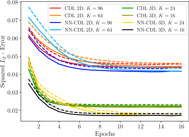
Figure 2 shows the training- and the validation-error during the optimization of the proposed network. As we can see, training the filters by back-propagation further reduced the error compared to using the pre-trained filters obtained by [3] and [8]. The effect is clearly more pronounced for the 3D case. Further, we see how drastic the impact of not carefully chosen and can be on CDL 2D and CDL 3D. Note that, although CDL-2D and CDL-3D in the end achieve results which are comparable with the proposed method, they only do so after a subsequent optimization of , and using the proposed INN. This demonstrates that the proposed INN can also be used as an algorithm for the selection of the regularization parameters.
| NRMSE | PSNR | SSIM | Params | |
|---|---|---|---|---|
| - | ||||
| CDL 2D [3] | 3 891 | |||
| NN-CDL 2D | 3 891 | |||
| CDL 3D [8] | 2 747 | |||
| NN-CDL 3D | 2 747 | |||
| NN-CAOL 3D [13] | 2 746 | |||
| DnCn3D [2] | 31 233 |
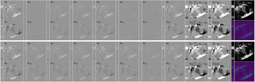
Because the proposed method is interpretable, we can verify that the learned filters indeed serve the purpose they were designed for. Figure 3 shows the estimates of at the last iteration of CDL 3D and NN-CDL 3D. We can see that indeed gives an approximation of the image and the approximation using the filters of NN-CDL 3D exhibits a lower point-wise error compared to CDL 3D.
V Conclusion
In this work, we have presented a physics-informed method for supervised training of a convolutional dictionary for image reconstruction applied to accelerated cardiac MRI. The proposed method consists of an iterative neural network (INN) which is rigorously derived from a properly defined sparse reconstruction problem. The filters of the dictionary are trained in a supervised manner. We have compared our method to two unsupervised model-agnostic methods and showed competitive results where, most importantly, our method does not require the choice of the regularization parameters as they are jointly trained with the filters. The proposed INN also achieved results comparable to its analysis operator counterpart and to a method based on deep INNs. On top, each learned component of the proposed reconstruction method is entirely interpretable in contrast to INNs with deep convolutional blocks.
References
- [1] Jonas Adler and Ozan Öktem, “Solving ill-posed inverse problems using iterative deep neural networks,” Inverse Problems, vol. 33, no. 12, pp. 124007, 2017.
- [2] Jo Schlemper, Jose Caballero, Joseph V Hajnal, Anthony N Price, and Daniel Rueckert, “A deep cascade of convolutional neural networks for dynamic MR image reconstruction,” IEEE Transactions on Medical Imaging, vol. 37, no. 2, pp. 491–503, 2018.
- [3] Jialin Liu, Cristina Carcia-Cardona, Brendt Wohlberg, Wotao Yin, “First-and second-order methods for online convolutional dictionary learning,” SIAM Journal on Imaging Sciences, vol. 11, no. 2, pp. 1589–1628, 2018.
- [4] Kerstin Hammernik, Teresa Klatzer, Erich Kobler, Michael P Recht, Daniel K Sodickson, Thomas Pock, and Florian Knoll, “Learning a variational network for reconstruction of accelerated MRI data,” Magnetic Resonance in Medicine, vol. 79, no. 6, pp. 3055–3071, 2018.
- [5] Andreas K Maier, Christopher Syben, Bernhard Stimpel, Tobias Würfl, Mathis Hoffmann, Frank Schebesch, Weilin Fu, Leonid Mill, Lasse Kling, and Silke Christiansen, “Learning with known operators reduces maximum error bounds,” Nature machine intelligence, vol. 1, no. 8, pp. 373–380, 2019.
- [6] Andreas Kofler, Markus Haltmeier, Tobias Schaeffter, and Christoph Kolbitsch, “An end-to-end-trainable iterative network architecture for accelerated radial multi-coil 2d cine MR image reconstruction,” Medical Physics, vol. 48, no. 5, pp. 2412–2425, 2021.
- [7] Vegard Antun, Francesco Renna, Clarice Poon, Ben Adcock, and Anders C Hansen, “On instabilities of deep learning in image reconstruction and the potential costs of AI,” Proceedings of the National Academy of Sciences, vol. 117, no. 48, pp. 30088–30095, 2020.
- [8] Il Yong Chun and Jeffrey A Fessler, “Convolutional dictionary learning: Acceleration and convergence,” IEEE Transactions on Image Processing, vol. 27, no. 4, pp. 1697–1712, 2017.
- [9] Vardan Papyan, Yaniv Romano, Jeremias Sulam, and Michael Elad, “Convolutional dictionary learning via local processing,” in Proceedings of the IEEE International Conference on Computer Vision, pp. 5296–5304, 2017.
- [10] Tran Minh Quan and Won-Ki Jeong, “Compressed sensing dynamic mri reconstruction using gpu-accelerated 3d convolutional sparse coding,” in International conference on medical image computing and computer-assisted intervention. Springer, pp. 484–492, 2016.
- [11] Stephen Boyd, Neal Parikh, Eric Chu, Borja Peleato and Jonathan Eckstein, “Distributed optimization and statistical learning via the alternating direction method of multipliers,” Foundations and Trends in Machine Learning, vol. 3, no. 1, pp. 1–122, 2011.
- [12] Brendt Wohlberg, “Efficient algorithms for convolutional sparse representations,” IEEE Transactions on Image Processing, vol. 25, no. 1, pp. 301–315, 2015.
- [13] Andreas Kofler, Christian Wald, Tobias Schaeffter, Markus Haltmeier, and Christoph Kolbitsch, “Convolutional analysis operator learning by end-to-end training of iterative neural networks,” in 2022 IEEE 19th International Symposium on Biomedical Imaging (ISBI), pp. 1 –5, 2022. doi=10.1109/ISBI52829.2022.9761621.
- [14] Matthew J Muckley, Ruben Stern, Tullie Murrell, and Florian Knoll, “Torchkbnufft: A high-level, hardware-agnostic non-uniform fast Fourier transform,” in ISMRM Workshop on Data Sampling & Image Reconstruction, 2020.